The Effect of 3D Transport-Induced Disequilibrium Carbon Chemistry on the Atmospheric Structure and Phase Curves and Emission Spectra of Hot Jupiter HD 189733b

Abstract

On hot Jupiter exoplanets, strong horizontal and vertical winds should homogenize the abundances of the important absorbers CH₄ and CO much faster than chemical reactions restore chemical equilibrium. This effect, typically neglected in general circulation models (GCMs), has been suggested as explanation for discrepancies between observed infrared lightcurves and those predicted by GCMs: On the nightsides of several hot Jupiters, GCMs predict outgoing fluxes that are too large, especially in the Spitzer 4.5 $\mu$m band. We modified the SPARC/MITgcm to include disequilibrium abundances of CH₄, CO and H₂O by assuming that the CH₄/CO ratio is constant throughout the simulation domain. We ran simulations of hot Jupiter HD 189733b with 8 CH₄/CO ratios. In the more likely CO-dominated regime, we find temperature changes $\geq$50-100 K compared to the equilibrium chemistry case across large regions. This effect is large enough to affect predicted emission spectra and should thus be included in GCMs of hot Jupiters with equilibrium temperatures between 600K and 1300K. We find that spectra in regions with strong methane absorption, including the Spitzer 3.6 and 8 $\mu$m bands, are strongly impacted by disequilibrium abundances. We expect chemical quenching to result in much larger nightside fluxes in the 3.6 $\mu$m band, in stark contrast to observations. Meanwhile, we find almost no effect on predicted observations in the 4.5 $\mu$m band, as the opacity changes due to CO and H₂O offset each other. We thus conclude that disequilibrium carbon chemistry cannot explain the observed low nightside fluxes in the 4.5 $\mu$m band.

1 Introduction

Close-in extrasolar giant planets, known as hot Jupiters, are the best characterized exoplanets to date. Due to their proximity to their host stars, they are expected to be tidally locked. This creates strong temperature contrasts between the permanent day side and the night side. For the temperature ranges of typical hot Jupiters, assuming chemical equilibrium, these temperature contrasts translate to large horizontal gradients in the abundance of methane (CH₄) and carbon monoxide (CO), two important infrared absorbers in the atmospheres of hot Jupiters. Carbon is preferentially found in CH₄ at high pressures and low temperatures, while at low pressures and high temperatures, CO is the dominant carbon-bearing species. Most models of hot Jupiters, especially three-dimensional general circulation models (GCMs) allowing for realistic representation of opacities and the effect that chemical composition exert on them, assume equilibrium chemistry as a basis for calculating opacities. However, the stark day-night temperature contrast also drives a vigorous atmospheric circulation, with a strong eastward equatorial jet advecting thermal energy from the day side to the night side and strong vertical mixing (e.g. Showman & Guillot, 2002; Showman & Polvani, 2011; Dobbs-Dixon & Lin, 2008; Heng et al., 2011; Thrastarson & Cho, 2011; Rauscher & Menou, 2012; Perna et al., 2012; Dobbs-Dixon & Agol, 2013; Parmentier et al., 2013; Mayne et al., 2014; Kataria et al., 2016; Mendonça et al., 2016). In addition, at low pressures ($\lesssim 1$ bar), the chemical time scale at which the interconversion between CH₄ and CO acts, becomes very long. Therefore, an air parcel is advected much faster than its CH₄ and CO abundances can adapt to the local equilibrium values. This process, called quenching, is expected to vertically and horizontally homogenize the abundances of CH₄ and CO (as well as of many other species, including N₂ and NH₃) in the near-infrared photospheres (located roughly between 1 bar and 1 mbar) of hot Jupiters (Cooper & Showman, 2006; Agúndez et al., 2012, 2014; Drummond et al., 2018b, a).

These disequilibrium abundances can have a significant effect on the opacities and thus the radiative transfer. Including this effect in general circulation models (GCMs) could potentially impact the thermal structure and atmospheric circulation, as well as the predicted spectra and phase curves. In fact, this has been proposed as a solution for the observed discrepancy between phase curves predicted by state-of-the-art GCMs assuming equilibrium chemistry and observations with the Spitzer Space Telescope (Knutson et al., 2012). GCMs over-predict the night side fluxes in the Spitzer 4.5 $\mu$m band for the hot Jupiters HD 189733b (Knutson et al., 2012), HD 209458b (Zellem et al., 2014) and WASP-43b (Stevenson et al., 2017). Within this wavelength bandpass, CO has a strong absorption band. For relatively cool hot Jupiters, like HD 189733b, transport-induced disequilibrium chemistry is expected to enhance the CO abundance on the night side compared to the equilibrium chemistry value (Cooper & Showman, 2006; Agúndez et al., 2014). Knutson et al. (2012) argued that this would lead to increased opacity in the 4.5 $\mu$m band, such that the outgoing radiation in that band would probe higher, cooler regions of the atmosphere, decreasing the flux emitted in this band. In addition to changing the pressure level from which the outgoing radiation is emitted, the altered opacities can also affect the thermal structure and the atmospheric circulation in a GCM, an effect not considered in the argumentation of Knutson et al. (2012). So far, this effect has only been taken into account by Drummond et al. (2018b, a).

The goal of this study is to better quantify how the combination of these two effects of disequilibrium carbon chemistry (the change in the level from which radiation escapes to space and the change in thermal structure) affects the thermal emission spectra predicted from GCMs. We assume that the abundance ratio of CH₄ to CO is constant throughout the entire simulation domain and treat the CH₄/CO abundance ratio as free parameter. This simple approach allows us to explore a broader parameter range than Drummond et al. (2018b, a) and to focus on the radiative effects. Our approach is justified by the findings of previous studies: Coupling a simple chemical relaxation scheme to a GCM of HD 209458b, both Cooper & Showman (2006) and Drummond et al. (2018b) found that the CO and CH₄ abundances are homogenized everywhere above the $\sim 3$ bar level. In a later study (published while this paper was in the peer-review process), Drummond et al. (2018a) find that the same is true for HD 189733b. Agúndez et al. (2014) instead used a full kinetical network in a pseudo-2D framework that was able to capture vertical and horizontal transport, and included photochemistry on the day side. They found that quenching homogenized the CO and CH₄ abundances at pressures between $\sim 1$ and $\sim 10^{-4}$ bars on HD 189733b. (At lower pressures, photochemical processes destroy CH₄ on the day side.) While these studies disagree on the relative importance of vertical versus horizontal quenching, all of them conclude that the abundances of CO and CH₄ should be homogeneous in the near-infrared photosphere, justifying our assumption.

However, coupling a chemical relaxation scheme to their GCM, Mendonça et al. (2018b) found that on WASP-43b, the CH₄ abundances were only homogenized horizontally but not vertically. A similar behavior is seen in the HD 209458b case of Agúndez et al. (2014) (though only for their nominal eddy diffusion profile). While there are several differences in the models and planet parameters used that could contribute to this different outcome, the perhaps most important factors are the hotter day side and the weak vertical mixing in both of these models. If horizontal transport dominates over vertical transport in setting the disequilibrium abundances, as these two papers find, whether abundances are homogenized only horizontally or vertically and horizontally depends on whether vertical quenching happens in the hottest region of the day side. Abundances thus are homogenized vertically and horizontally if in the hottest regions of the day side the vertical mixing time scale is shorter than the chemical time scale. If vertical mixing is very weak or the day side is too hot (leading to a shorter chemical time scale), this condition is not fulfilled and abundances are only homogenized horizontally but not vertically. In the case of Agúndez et al. (2014), the hotter day side compared to Drummond et al. (2018b) at low pressures is largely due to their assumption of a thermal inversion on the day side of HD 209458b. Mendonça et al. (2018b) look at WASP-43b, for which Kataria et al. (2015) also found a larger day-night contrast and hotter day side compared to HD 209458b due to its shorter orbital period and larger gravity. Our study looks at HD 189733b, which has a significantly lower zero-albedo equilibrium temperature than HD 209458b and WASP-43b. Since the chemical time scale dramatically increases with decreasing temperature, it is likely that abundances are homogenized horizontally and vertically on this planet, and both published studies looking at HD 189733b confirm this (Agúndez et al., 2014; Drummond et al., 2018a).

With the focus of these previous studies being on chemistry, most of them did not self-consistently calculate the radiative transfer, and thus were not able to quantify the effect of the changed opacities on the temperature structure in their model. In their GCM, Cooper & Showman (2006) used a Newtonian cooling scheme, in which the temperature relaxes towards a prescribed temperature profile at each point in the atmosphere. Like typical kinetical networks, Agúndez et al. (2014) used a prescribed background pressure-temperature profile (in this case derived from a GCM assuming equlibrium chemistry). Mendonça et al. (2018b) use a double-grey radiative transfer scheme. Only Drummond et al. (2018b) and Drummond et al. (2018a), whose GCM uses state-of-the-art radiative transfer with correlated k-coefficients, included the effect of the changed opacities on the temperature structure in a GCM. Our approach complements previous studies by focusing on the radiative transfer rather than on chemistry. The photospheric disequilibrium CH₄ and CO abundances found in coupled chemistry-circulation models such as Drummond et al. (2018b) strongly depend on the temperature profile in transition region between equilibrium chemistry and disequilibrium chemistry ($\sim 1$ to 10 bars)(Moses et al., 2011; Venot et al., 2014). However, the temperature profile in this region depends on the initial temperature profile used in the GCM (Amundsen et al., 2016), assumptions about the interior heat flux (e.g., Guillot & Showman, 2002; Burrows et al., 2003; Fortney et al., 2008) and dissipation in deep layers (e.g., Guillot & Showman, 2002; Tremblin et al., 2017; Komacek & Youdin, 2017) . Furthermore, typical GCM simulations only resolve dynamic mixing through the large-scale circulation. If unresolved sub-grid-scale turbulence is relevant near the quench level (e.g., Menou, 2019), it might further alter the quenched abundances. Uncertainties in reaction rates can also affect the resulting abundances (e.g., Visscher & Moses, 2011). Overall, although it is well established that the CH4/CO ratio should be reasonably homogenized throughout the photosphere, many unconstrained factors will determine the actual value of this ratio. Studying how the thermal response and the resulting emission spectra and phase curves depends on the CH₄/CO ratio, as is our goal, thus adds to the overall understanding of the effects of disequilibrium chemistry.

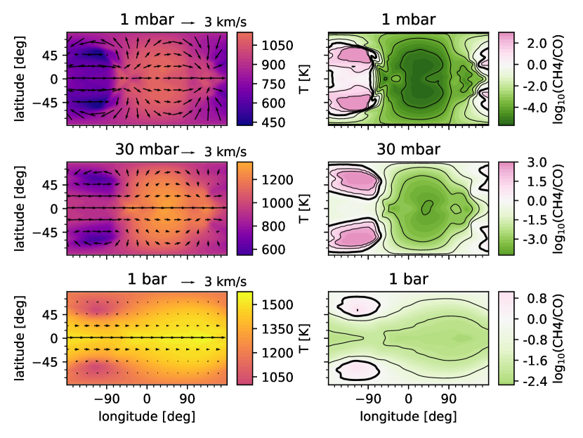
Figure 1: Left: horizontal temperature maps of the reference simulation (equilibrium chemistry) at pressures of 1 mbar, 30 mbars and 1 bar, respectively. The substellar point (0 ^∘ longitude, 0 ^∘ latitude) is at the center of each panel. The arrows represent the velocities of the horizontal component of the wind. Right: horizontal maps of the abundance ratio of methane to carbon monoxide assuming chemical equilibrium. Methane dominated regions are magenta while carbon-monoxide dominated regions are green. The contours are evenly spaced in log space and mark log₁₀(CH₄/CO)=(-4,-3,-2,-1,0,1, 2), respectively. The zero contour (corresponding to CH₄/CO=1) is thickened.

We choose to focus on HD 189733b. Due to its cooler temperature compared to HD 209458b and WASP-43b, disequilibrium effects are expected to be stronger on this planet. The latter two planets are hot enough that in simulations assuming equilibrium chemistry, CO is the dominant carbon species at all longitudes and latitudes (Showman et al., 2009; Drummond et al., 2018b). In contrast, on the cooler HD 189733b, in chemical equilibrium one expects that the day side is dominated by CO, while the night side is dominated by CH₄ (see Figure 1). HD 189733b thus occupies an interesting point in the parameter space: Regardless of the quenched CH₄ and CO abundances, including disequilibrium chemistry will change which of the two species is dominant on about half of the planet. The radiative effects of disequilibrium chemistry are thus expected to play a larger role than on hotter planets. In addition, unlike for HD 209458b, for HD 189733b there exist phase curve observations in multiple Spitzer bandpasses (Knutson et al., 2007, 2009; Agol et al., 2010; Knutson et al., 2012), providing stronger observational constraints.

2 Methods

We use the SPARC/MITgcm model (Showman et al., 2009) to perform simulations of hot Jupiter HD 189733b. This model couples the two-stream, non-gray radiative transfer code of Marley & McKay (1999) to the MITgcm general circulation model of Adcroft et al. (2004) and has previously been applied to a wide range of hot Jupiters and other exoplanets (e.g., Showman et al., 2009, 2013, 2015; Parmentier et al., 2013, 2018; Lewis et al., 2010, 2014; Kataria et al., 2013, 2014, 2015).

Table 1: Model parameters

Parameter	Value	Units
Radius	$7.9559\cdot 10^{7}$	m
Gravity	22.86	m s-2
Rotation period	2.22	d
Semimajor axis	0.03142	AU
Specific heat capacity	$1.3\cdot 10^{4}$	J kg-1 K-1
Specific gas constant	3714	J kg-1 K-1
Interior flux	0	W m-2
Horizontal resolution	C32
Vertical resolution	53	layers
Lower pressure boundary	$2\cdot 10^{-6}$	bar
Upper pressure boundary	200	bar
Hydrodynamic time step	25	s
Radiative time step	50	s

2.1 Dynamics

Using the MITgcm (Adcroft et al., 2004), we solve the three-dimensional global primitive equations on a cubed sphere grid. The primitive equations are valid for stably stratified shallow atmospheres. Horizontal noise is smoothed with a fourth-order Shapiro filter (Shapiro, 1970).

The key model parameters are summarized in Table 1. We assume a gravity of $g=22.86$ m s^-2, a planetary radius of $7.9559\cdot 10^{7}$ m and a rotation period equal to the orbital period of 2.22 days, as the planet is assumed to be in synchronous rotation. We use a value of $c_{p}=1.3\cdot 10^{4}$ J kg^-1 K^-1 for the specific heat capacity and $\kappa=R/c_{p}=2/7$, where $R$ is the specific gas constant. These values are appropriate for hydrogen dominated atmospheres. Our simulations use a horizontal resolution of C32, which is roughly equivalent to a resolution of 128x64 on a longitude-latitude grid. The pressure spans from 200 bars to 2 $\mu$bar and is resolved by 53 vertical levels. We use a timestep of 25 s, run the simulations for 1,000 days and then average over the last 100 days. Convergence tests in previous studies using the SPARC/MITgcm have shown that simulations have sufficiently converged at that point. Specifically, the emitted infrared flux changes by less than a few percent between integration times of $\approx 1,000$ days and $\approx 4,000$ days. (Showman et al., 2009, Fig. 12).

2.2 Radiative transfer

The radiative transfer code in our model is based on the plane-parallel code of Marley & McKay (1999). This code was originally developed to study Titan’s atmosphere (McKay et al., 1989) and has since been applied to Uranus (Marley & McKay, 1999) , brown dwarfs (Burrows et al., 1997; Marley et al., 1996, 2002) and hot Jupiters (Fortney et al., 2005, 2008; Showman et al., 2009). The code uses the delta-discrete ordinate method (Toon et al., 1989) for the incident stellar flux, while the thermal flux is calculated using the two-stream source function method (also of Toon et al., 1989). Molecular opacities are treated using the correlated k-method (e.g. Goody & Yung, 1989): In each frequency bin, the opacity information from line-by-line calculations using as many as 10,000 to 100,000 frequency bins is turned into a cumulative distribution of opacities, which is then described by 8 k-coefficients. We use 11 frequency bins spanning from 0.26 $\mu$m to 325 $\mu$m (see Kataria et al., 2013). The correlated-k method is the most sophisticated and accurate treatment of opacities in GCMs of exoplanets to date and is used both in the SPARC/MITgcm and in the adaptation for hot Jupiter of the UK MetOffice model (Amundsen et al., 2016).

In order to combine the opacities from different species within the atmosphere, we employ the approach of pre-mixed opacities, meaning that the k-coefficients of the mixture are derived from line-by-line opacities that are calculated for a mixture with specified chemical abundances that are specified functions of temperature and pressure (typically derived from equilibrium chemistry). This approach is fast and accurate. We use the equilibrium chemistry abundances for solar metallicity of Lodders & Fegley (2002) and Visscher et al. (2006) with the modifications for CH₄, CO and H₂O described in section 2.3 and the opacities of Freedman et al. (2008) including the updates of Freedman et al. (2014). Note that the updated opacities result in changes in the thermal structure and the resulting equilibrium chemistry phase curve compared to Showman et al. (2009) and Knutson et al. (2012) (see Section 4.2). The disadvantage of this method is that it leaves little flexibility for varying abundances due to disequilibrium chemistry. However, alternative methods combining the k-coefficients of individual species on the fly come at a much higher computational cost and are thus impractical when coupled to GCMs (as discussed in Amundsen et al., 2017). To explore the effect of disequilibrium abundances, we thus take advantage of the fact that due to strong horizontal and vertical mixing, the disequilibrium abundances of CH₄ and CO are expected to be close to constant throughout the photosphere, as further detailed in section 2.3.

To obtain spectra and phase curves, we postprocess our simulation output using the same plane-parallel two-stream radiative transfer code as used in our full 3D simulations, but adopting 196 wavelength bins instead of 11 to yield improved spectral resolution. Given the time-averaged temperature structure from the GCM at a particular time, we calculate the outgoing flux in the line of sight to the observer for each atmospheric column. The fluxes are then combined into a weighted average across the disk to give the total flux received at a particular observing vantage point and at a particular time during the orbit. We do this calculation at many orbital phases (throughout which the Earth-facing hemisphere shifts in longitude) to assemble full orbit phase curves at wavelengths of interest. This method is similar to the method described in Fortney et al. (2006), Showman et al. (2009) and Parmentier et al. (2016) and naturally takes into account limb darkening of the planet. We use a NextGen spectrum (Hauschildt et al., 1999) for HD 189733, a stellar radius of 0.805 $R_{\odot}$ (Boyajian et al., 2015) and a planet-to-star radius ratio $R_{p}/R_{\ast}=0.0145$.

2.3 Disequilibrium chemistry

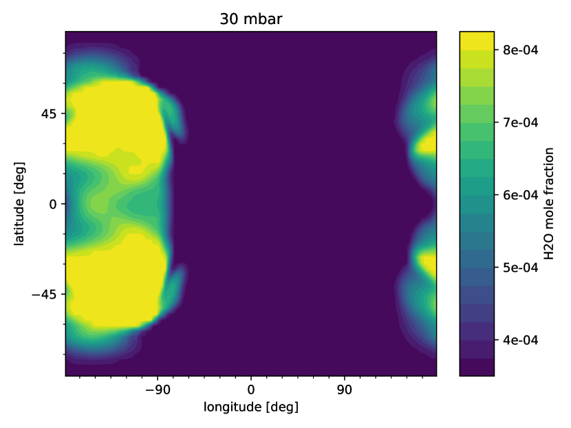
Figure 2: Water abundance at the 30 mbar level in the equilibrium chemistry simulation. The substellar point is at the center of the panel. In disequilibrium chemistry, in contrast, the abundances are expected to be homogenized between the day- and night side of the planet.

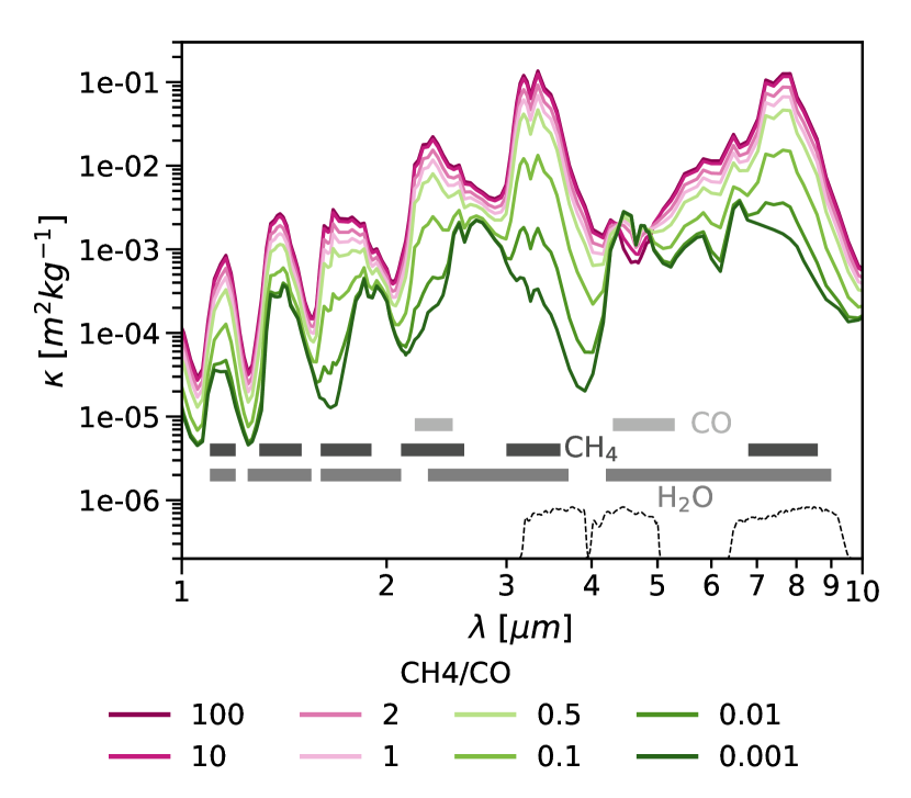
Figure 3: Opacities for different CH₄/CO ratios at a temperature of 1000 K and a pressure of 30 mbar. Opacities for CH₄ dominated ratios are plotted in magenta and CO dominated ratios are plotted in green. The locations of imporant absorption bands are shown as grey bars towards the bottom of the figure. The dashed black lines indicate the filter sensitivity profiles for the Spitzer 3.6 $\mu$m, 4.5 $\mu$m and 8 $\mu$m bands.

All previous studies of hot Jupiters using the SPARC/MITgcm utilized k-coefficient tables calculated assuming equilibrium chemistry. To explore the effect of transport-induced disequilibrium carbon chemistry, in this study we instead assume that the CH₄ to CO ratio is quenched to a constant value throughout the entire atmosphere. This assumption is a good approximation at pressures lower than roughly 1 to 10 bars, as shown by Cooper & Showman (2006), Agúndez et al. (2014) and Drummond et al. (2018b, a). At higher pressures, the chemical timescale becomes shorter than the mixing time scale and the approximation of a constant quenched value breaks down. Since this study focuses on the effect on the outgoing radiation in the near infrared, which probes pressures beween 1 mbar and 1 bar (see Fig. 9 in Showman et al. (2009) and Fig. 12 and 14 in Moses et al. (2011), we believe this approximation is justified. The deep regions of the atmosphere (deeper than 10 bars) also have extremely small net fluxes compared to the fluxes in the observable atmosphere (where the incoming starlight is absorbed and radiation is escaping to space), and so the dynamics in the observable atmosphere are not strongly sensitive to modest changes in the opacities and fluxes in the deep ($p>$10 bar) atmosphere. In addition, because of the low net fluxes, the error in opacity we make by extending constant CH₄/CO ratios to the deep atmosphere is expected to have a relatively small effect on the temperature structure. We expect the error in the temperature profile in the deep atmosphere to be smaller than, or at most comparable to, the uncertainty due to the unknown internal heat flux of hot Jupiters and certainly smaller than the error due to the limited integration time. (Because of the low net fluxes and long radiative time scales in the deep atmosphere, the time it takes for 3D GCM simulations to converge in the deep atmosphere far exceeds simulation runtimes feasible with state-of-the-art computational facilities. This problem is not unique to our model, but universal to 3D GCMs of hot Jupiters when realistic radiative transfer is included.)

Our approximation of a constant CH₄/CO ratio also breaks down at pressures lower than $\sim 10^{-4}$ bars, as on the day side CH₄ is destroyed photochemically in these regions (Moses et al., 2011; Agúndez et al., 2014). Again, this process is not expected to affect the broadband emission spectra that we are interested in or the temperatures in the regions probed by broadband emission.

The quenched CH₄/CO ratio can in general be constrained by comparing the chemical time scale and the mixing time scale. In a 1D picture, the quenched abundances are approximately given by the abundances at the point at which both time scales are equal. In practice, however, the vertical mixing time scale in 1D and 2D models depends on the assumptions about the strength of vertical mixing (parametrized through the eddy diffusion coefficient $K_{zz}$) and the chemical time scale depends on the reaction rates, some of which are not well-known in the pressure and temperature range encountered in hot Jupiter atmospheres. A variety of different 1D and pseudo-2D thermochemical kinetics models of HD 189733b find CH₄/CO ratios roughly between 0.001 and 0.5 (Moses et al., 2011; Visscher & Moses, 2011; Agúndez et al., 2014; Drummond et al., 2016). However, CH₄/CO ratios larger than one might also be possible if vertical mixing is very strong (Tsai et al., 2018). GCM simulations with simplified chemical schemes have focused on the hotter HD 209458b and find CH₄/CO ratios $\sim$ 0.01 (Cooper & Showman, 2006; Drummond et al., 2018b). For HD 189733b, Drummond et al. (2018a) find CH₄/CO ratios between 0.1 and 0.2. We thus choose to treat the CH₄/CO ratio as a free parameter and perform 8 simulations varying this ratio from 0.001 to 100 as well as a reference simulation assuming equilibrium chemistry. Although kinetics models favor CH₄/CO ratios $<1$, we include the full range for completeness.

2.3.1 Water and CO₂ abundances

The net reaction that converts CH₄ to CO and vice versa is

$$\text{CH}_{4}+\text{H}_{2}\text{O}\rightleftharpoons\text{CO}+3\text{H}_{2}.$$ (1)

Together with the CH₄ and CO abundances, the water abundance thus changes as well. CO and H₂O are the only major oxygen-bearing species in the region where quenching dominates the abundances (Moses et al., 2011), and the total number of oxygen atoms has to be preserved. As a consequence, when reaction (1) is quenched, the water abundance is frozen to a constant value as well. This value is directly tied to the CH₄ and CO abundances (e.g., Moses et al., 2011, Fig. 4, 5 and 8). As long as either CO or CH₄ dominates over the other, a change in the CH₄/CO ratio results in only a marginal change in the water abundance. However, when transitioning from the CO-dominated to the CH₄ dominated regime, the water abundance varies by a factor of $\approx 2$. Assuming equilibrium chemistry, the water abundance thus varies by this factor of $\approx 2$ between the day- and night side of HD 189733b, as can be seen in Figure 2. Including horizontal and vertical transport, however, the water abundance is expected to remain constant between day- and night side due to quenching (Agúndez et al., 2014, Fig. 12). Since water is such an important infrared absorber, it is necessary to adjust the water abundance in our model to reflect this. We achieve this by adjusting the water abundance such that the total number of oxygen atoms present in water and CO is conserved. The C/H and O/H ratios thus remain at solar values, consistent with our general assumption of solar elemental abundances.

We leave the abundance of CO₂ unchanged from its equilibrium chemistry value, as it is not the dominant carbon species in either equilibrium or disequilibrium chemistry and deviations from equilibrium chemistry are expected to remain moderate compared to CH₄ (Agúndez et al., 2014).

2.3.2 Changes in Opacity

To illustrate the changes in opacity, the resulting near-infrared opacities for different CH₄/CO ratios at a typical photospheric pressure and temperature are shown in Figure 3. The plotted opacities represent the bin-averaged opacity for each of the 196 wavelength bins used for the postprocessing averaged over the inverse of the opacity. This kind of average is a good way of representing the effects on the broadband emission. Note that the average is only used for illustration in the figure—in the radiative transfer in the GCM and for post-processing we use the correlated-k method instead (with 11 and 196 bins, respectively). It is obvious from Figure 3 that for a higher CH₄/CO ratio, the opacity significantly increases for almost all wavelengths in the near and mid-IR. This is mainly because CH₄ has many broad absorption bands in the near- and mid-infrared while CO only has a few narrow absorption bands. On top of that, with increased CH₄, the water abundance also increases by a factor of $\sim 2$. Similar to CH₄, water has many broad absorption bands. The only spectral region in which the opacity decreases for high CH₄/CO ratios is near the CO absorption band centered around 4.7 $\mu$m. Even in this region, the opacity decreases only by a factor of $\sim$2, much less than it increases at most other wavelengths. This is likely because the water feature centered around 6.3 $\mu$m contributes significantly to the total opacity in this region. Since for every CO molecule that is removed, a water molecule is added, these two changes in opacity partially offset each other in this region.

3 Results

3.1 Reference simulation: equilibrium chemistry case

First, we give a brief overview of the reference simulation, which assumes equilibrium chemistry. The left column of Figure 1 shows the temperature and horizontal wind velocities at pressures of 1 mbar, 30 mbars and 1 bar. The pressure levels in the figure are chosen such that the lowest pressure level shown (1 mbar, uppermost panel) is slightly above the photosphere at most infrared wavelengths, while the highest pressure level (1 bar, lowermost panel) is somewhat below the photosphere at most infrared wavelengths. The temperature and wind patterns are typical for a hot Jupiter: The simulation exhibits a large day-night temperature contrast, especially at low pressures, and a superrotating (eastward) equatorial jet. The hottest point is shifted east with respect to the substellar point. The coldest regions in the simulation are east of the antistellar point at roughly 40^∘ to 50^∘ latitude, at the center of two large gyres.

At low pressures, where the radiative time scale is short compared to the dynamical time scale, the temperature difference between day- and night side is largest. In addition to the jet, there is a strong day-to-night flow. As pressure increases and the radiative timescale becomes longer, the eastward equatorial jet dominates more over the day-to-night flow. At a pressure of 1 bar, the equatorial jet efficiently transports heat from the day side to the night side and longitudinal temperature differences along the equator are small. Winds at mid-latitudes are much smaller than at lower latitudes. The cold spots associated with the night side gyres are still several hundred K colder than the equatorial regions.

The ratio of the equilibrium chemistry abundances of CH₄ to CO is plotted in the right column of Figure 1. In chemical equilibrium, CH₄ is the dominant carbon species at high pressures and low temperatures, while carbon preferentially forms CO at low pressures and high temperatures. On isobars, abundances thus directly follow the temperature pattern. On the day side, CO is the prevailing carbon species and is up to 5 orders of magnitude more abundant than CH₄. At most locations of the night side, the abundances of both species become more even, with CH₄ prevailing. Methane abundances peak at the night side cold spots at mid-latitudes. As with temperature gradients, the abundance gradients become much less pronounced deeper in the atmosphere: While the abundance ratios span over 8 orders of magnitude at the 1 mbar level, they differ by only 3 orders of magnitude at the 1 bar level.

3.2 Simulations with quenched abundances: Thermal structure

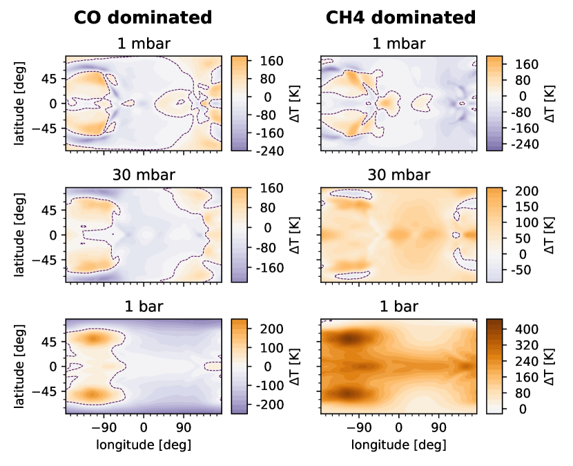
Figure 4: Temperature difference of the time-averaged simulation output with respect to the equilibrium chemistry simulation for two simulations with a quenched CH₄/CO ratio (left: CH₄/CO=0.01, right: CH₄/CO=100) at pressures of 1 mbar, 30 mbars and 1 bar. Positive temperature differences (i.e. quenched simulation is hotter) are shown in orange, negative temperature differences are purple. Dashed lines indicate the zero contour.

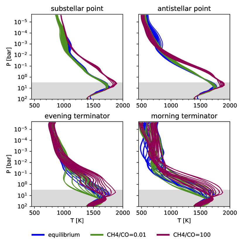
Figure 5: Pressure-temperature profiles. The equilibrium chemistry simulation is shown in blue, the CH₄/CO=0.01 simulation in green and the CH₄/CO=100 simulation in magenta. The shaded grey region indicates pressure ranges for which the simulation has not converged due to the long radiative timescale in deep layers of the atmosphere. Coincidentally, our assumption of a constant quenched CH₄/CO ratio breaks down at roughly a similar pressure. Upper left: Profiles within 10^∘ of the substellar point. Upper right: Profiles within 10^∘ of the antistellar point. Lower left: Profiles within $\pm 2^{\circ}$ of the evening terminator. Lower right: Profiles within $\pm 2^{\circ}$ of the morning terminator. The temperature profiles in this figure are available as Data behind the Figure.

In response to the different opacities, the thermal structure changes in the simulations with disequilibrium chemistry compared to the reference case. We consider two of the quenched simulations, CH₄/CO=0.01 and CH₄/CO=100, in detail to illustrate these changes for the CO dominated and the CH₄ dominated regime. Figure 4 shows the temperature difference with respect to the reference case on isobars. Vertical pressure-temperature profiles from these two simulations along with the reference simulation are plotted in Figure 5.

In the CO dominated regime (the regime favored by kinetics models), the day side is cooler compared to the equilibrium case, while the temperature of large parts of the night side, including the midlatitude cold spots, increases. Temperatures also drop at high latitudes, especially on the night side. All of these effects can be seen in the left column of Figure 4. In the particular case shown (CH₄/CO=0.01), day side temperatures drop by about 50 K throughout most of the photosphere. This is also evident in the pressure-temperature profiles near the substellar point (upper left panel of Figure 4). A closer look at the pressure-temperature profiles reveals that the vertical temperature gradient is slightly larger compared to the equilibrium chemistry case near the substellar point, but slightly smaller at the antistellar point. This is likely because on the day side, greenhouse gases (CH₄, H₂O) are added compared to the equilibrium composition while on the night side greenhouse gases are taken away. The CH₄/CO=0.001 simulation (not shown) displays very similar changes in thermal structure, but with a somewhat larger amplitude.

Our interpretation for why the day side is cooler is related to energy-balance: The changes in opacity lead to only slight changes in albedo, so for all the CH4/CO ratios considered, the total amount of absorbed starlight is nearly the same. Since the simulations achieve an approximate energy balance (energy gained equals energy lost), this means that the total IR energy radiated to space (from the entire planet) is also nearly the same regardless of the CH₄/CO ratio. Compared to equilibrium chemistry, the overall infrared opacity decreases on the night side. Therefore, the radiation on the night side escapes to space from deeper levels, where the atmosphere tends to be hotter, leading to a larger flux being radiated away. As a consequence, less energy is returned to the day side and the day side cools, which in turn leads to a dayside radiating less IR flux.

In the (less likely) CH₄ dominated case, the temperature changes are more striking: Below roughly the 10 mbar level, temperatures are significantly hotter at almost all longitudes and latitudes. In the CH₄/CO=100 simulation, the temperature difference with respect to the reference simulation reaches 200 to 400 K at the 1 bar level in the equatorial region (see right column of Figure 4). In this simulation, the location of the night side cold spots shifts to slightly higher latitudes. In Figure 4, this is visible in the center right panel as the light blue regions and in the upper right panel as the two small deep purple regions at $\approx\pm 60^{\circ}$ latitude in conjunction with two orange regions at lower latitudes.

At the 1 mbar level, temperatures are similar or slightly colder compared to the reference simulation. Looking at the temperature profiles in Figure 5, it is obvious that the temperature gradient between 1 mbar and 1 bar is steeper in the CH₄ dominated case than for the other simulations at all four locations shown, signifying a stronger greenhouse effect. Given that in the CH₄ dominated case the abundances of the greenhouse gases methane and water are enhanced compared to equilibrium chemistry by several orders of magnitude and a factor of $\sim 2$, respectively, at any location other than the night side mid-latitude cold spots, this behavior is expected.

3.3 Phase Curve Predictions and Comparison with Observations

We post-process the GCM results as described in Section 2.2 to obtain phase curves and emission spectra and compare them to the available observational data (Figure 6). In short, the fit with respect to the observational phase curve worsens substantially in the 3.6 $\mu$m band for all quenched ratios while the changes in the 4.5 $\mu$m band are negligible in the expected CO dominated case and lead to a worse fit in the CH₄ dominated regime.

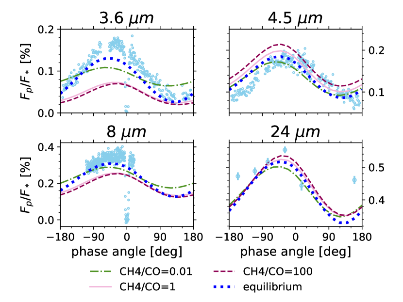
Figure 6: Phase curves predicted from our models and available observational data in the Spitzer 3.6, 4.5, 8 and 24 micron bands. The green dash-dotted line represents the CH₄/CO=0.01 simulation, the light pink solid line CH₄/CO=1, the magenta dashed line CH₄/CO=100 and the thick dotted blue line the reference simulation. The observational data (light blue circles) are the same as in Fig. 12 in Knutson et al. (2012) and are taken from Knutson et al. (2012) (3.6 and 4.5 $\mu$m), Knutson et al. (2007, 2009); Agol et al. (2010) (8 $\mu$m) and Knutson et al. (2009) (24 $\mu$m). All model phase curves in this figure are available as Data behind the Figure.

In the 3.6 $\mu$m band, the phase curve amplitude decreases for all quenched simulations compared to equilibrium chemistry. A similar, but less drastic behavior can be seen in the 8 $\mu$m band. This behavior is expected for wavelength regions with strong methane absorption bands, including these two band passes: In equilibrium chemistry, the outgoing radiation on the day side, where there is little methane, probes deeper, hotter layers while on the night side, where more methane is present, the radiation is emitted from higher, cooler layers. Thus the temperature varies more strongly from day to night on the photosphere in these bands (which differs in pressure from day to night) than it does on isobars. This enhances the day-night contrast of the phase curve relative to what would occur if the photosphere were at constant pressure (see also Dobbs-Dixon & Cowan, 2017). When assuming a constant methane abundance throughout the atmosphere, however, regardless of the exact value, the outgoing radiation emerges from similar pressure regions everywhere on the planet and the phase curve amplitude decreases. Consistent with this picture, the day side fluxes from the CH₄/CO=0.01 simulation are relatively close to those from the equilibrium chemistry simulation, while the night side fluxes from the CH₄ dominated simulations match those from equilibrium chemistry at the flux minimum.

In the 4.5 $\mu$m band, the night side fluxes are similar to or higher than the value from the equilibrium chemistry simulation for all quenched values. At first, this seems surprising, given that Knutson et al. (2012) base their argument for disequilibrium chemistry almost entirely on the fact that equilibrium chemistry models over-predict the 4.5 $\mu$m night side fluxes, arguing that adding CO on the night side will shift the photosphere in this band to a higher, colder atmospheric layer and thus decrease the flux. However, they ignore that when changing the CO abundance through quenching, the water abundance should also change. Water has significant opacity in the 4.5 micron band as well. Averaged across the band, its molecular absorption cross section is comparable to that of CO (see e.g. Figure 5 in Fortney et al. (2006) or Figures 2 and 3 in Sharp & Burrows (2007)). For each CO molecule added, an H₂O molecule is removed (assuming metallicity is held constant), and the resulting changes in opacity in the 4.5 micron band due to CO and H₂O largely offset each other (see also Section 2.3 and Figure 3). The changes in the 4.5 micron phase curve are thus mainly due to the change in thermal structure and not due to a change of the photospheric level. In the hotter CH₄ dominated case, the flux increases at all phase angles in this band. In the CO dominated case, the flux near the phase curve maximum decreases slightly compared to the equilibrium chemistry case, reflecting the cooler day side, while the phase curve follows closely the equilibrium chemistry phase curve at other phase angles.

In the 24 $\mu$m band, the difference between the disequilibrium and equilibrium chemistry simulations is relatively small. None of the predicted phase curves match the available data on the night side well. However, as observations in this band do not cover all phase angles, the shape of the phase curve in this band remains uncertain.

3.4 Phase Curve Trends

We now examine trends in the phase curve properties with the quenched ratio. Two factors control how the phase curve in the quenched case differs from the the equilibrium chemistry case. First, the change in opacities directly impacts the thermal structure of the planet, as discussed in Section 3.2. Second, the change in opacities causes the photospheric level to shift upwards or downwards. As a result, the outgoing radiation probes cooler or hotter layers. This change in the location of the photosphere can also be studied by postprocessing the output of GCM simulations assuming equilibrium chemistry with quenched opacities instead of self-consistently including quenched opacities in the GCM. It is thus of significant interest to examine the relative importance of both of these factors in shaping the predicted phase curve. If it turned out that the change in the thermal structure had only a small effect on the phase curve, modelers could restrict themselves to including disequilibrium chemistry in the postprocessing of the GCM output, which is simpler and computationally less expensive. In addition to computing the phase curves from the simulations with disequilibrium chemistry (self-consistent opacities), we thus also computed phase curves by postprocessing the output from the equilibrium chemistry simulation with quenched opacities.

Figures 7 to 9 show trends in secondary eclipse depth, phase curve offset and phase curve amplitude, respectively, with the quenched ratio for phase curves obtained from both simulations with self-consistent opacities and from the equilibrium chemistry simulation postprocessed with quenched opacities. If both curves align, the change is dominated by the shift in the photosphere pressure. If there are large discrepancies between the postprocessed and the self-consistent GCM phase curves, the change in thermal structure plays an important role.

In the 3.6 and 8 $\mu$m bands, which include strong methane absorption features, the phase curve amplitude increases with increasing methane abundance (Figure 9), while the phase curve offset and the secondary eclipse flux decrease (Figures 8 and 7, respectively). This is expected as the photosphere in these bands shifts to higher levels of the atmosphere with stronger day-night contrasts. All of these trends flatten once CH₄ starts to dominate over CO. The phase curve amplitudes from the post-processed simulations closely match the ones with self-consistent opacities, indicating that the change of the photospheric level is the dominant cause for this trend. For the phase curve offset, the direction of the trend is similar; however, the trend is weaker in the post-processed only points, indicating that the change in thermal structure significantly contributes to the trend.

In the 4.5 $\mu$m band, secondary eclipse flux, phase curve offset and phase curve amplitude from the postprocessed-only simulations are close to the equilibrium value, indicating that the location of the photosphere changes only marginally. In the simulations with self-consistent opacities, however, the secondary eclipse flux is increasing with increased methane abundance, in line with the hotter temperatures in the simulation described in Section 3.2. The phase curve offset also decreases with increasing CH₄ in the CO dominated regime. The phase curve amplitudes stay similar.

In the 24 $\mu$m band, there are no trends in secondary eclipse and phase curve amplitude. For the phase curve offset, the simulations with self-consistent opacities replicate the same decreasing trend as in other wavelength bands, as would be expected for a trend due to a change in thermal structure.

It is also of interest to examine how the described trends compare to the properties of the observed phase curve (indicated in black with grey error bars in Figures 7 to 9). In the 3.6 $\mu$m and 8 $\mu$m bands, the secondary eclipse depth is closer to the observed value for low CH₄/CO values than for high CH₄/CO values. The phase curve offset, in contrast, matches the observed value for CH₄/CO values near 0.5 in the 3.6 $\mu$m band and is closest to the observed value for CH₄/CO values greater than one for the 4.5 $\mu$m and 8 $\mu$m bands. The phase curve amplitude in the 3.6 $\mu$m band is closer to the observed value for high CH₄/CO ratios. In short, among the quenched simulations there is no one CH₄/CO ratio that matches the phase curve properties best, as low CH₄/CO ratios match the secondary eclipse better but high CH₄/CO ratios match the phase curve offset better. This further underlines our finding from Section 3.3 that quenching of CH₄ and CO does not provide a good explanation for the shape of the observed phase curves.

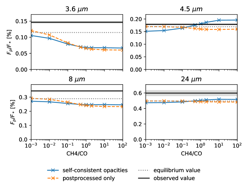
Figure 7: Secondary eclipse depths for different quenched CH₄/CO ratios. Values from the GCM simulations including the quenched opacities are shown as blue crosses connected by a solid line, while values obtained from postprocessing the equilibrium chemistry simulation are shown as orange crosses connected by a dashed line. The equilibrium value is indicated by the dashed grey line and the observed values from Knutson et al. (2012) are shown as a solid black line with the 1$\sigma$ errors shaded in grey.

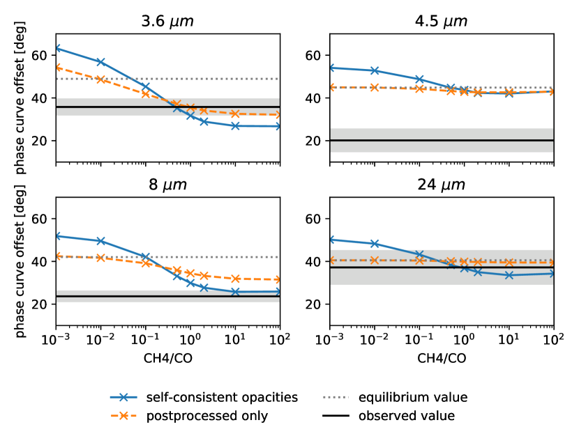
Figure 8: Eastward offsets of the maximum flux with respect to secondary eclipse for different quenched CH₄/CO ratios. Values from the GCM simulations including the quenched opacities are shown as blue crosses connected by a solid line, while values obtained from postprocessing the equilibrium chemistry simulation are shown as orange crosses connected by a dashed line. The equilibrium value is indicated by the dashed grey line and the observed values from Knutson et al. (2012) are shown as a solid black line with the 1$\sigma$ errors shaded in grey.

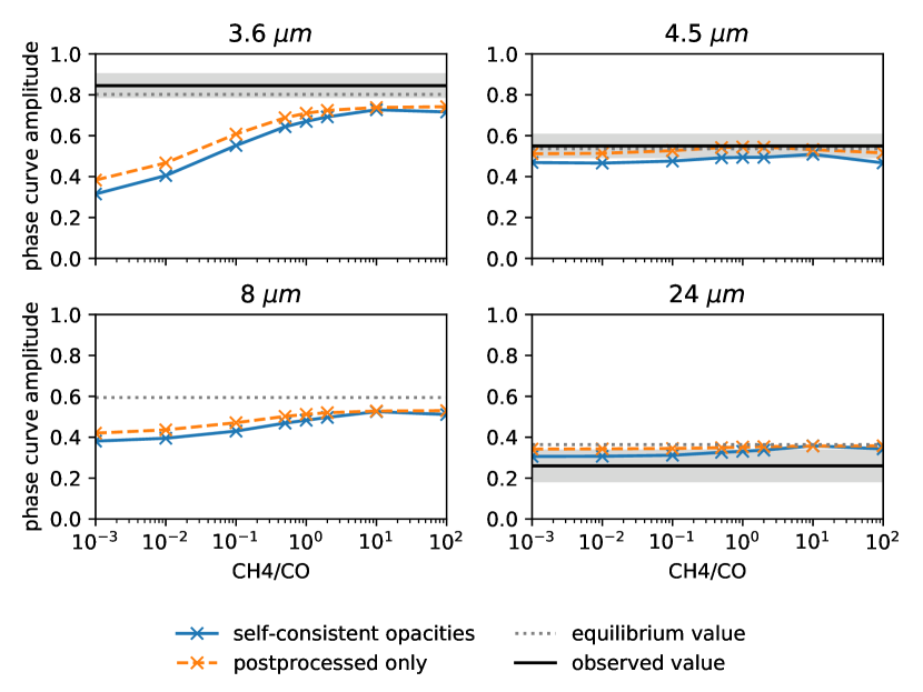
Figure 9: Normalized phase curve amplitudes, defined as $A=1-F_{min}/F_{max}$, for different quenched CH₄/CO ratios. Values from the GCM simulations including the quenched opactities are shown as blue crosses connected by a solid line, while values obtained from postprocessing the equilibrium chemistry simulation are shown as orange crosses connected by a dashed line. The equilibrium value is indicated by the dashed grey line and the observed values from Knutson et al. (2012) are shown as a solid black line with the 1$\sigma$ errors shaded in grey. Note that for the 8 $\mu m$ band there is no observed value, as observations in this band did not cover the night side.

3.5 Emission spectra

To move beyond a discussion restricted to the Spitzer bands, we plot the predicted emission spectra of the day side (Figure 10) and night side (Figure 11) for the CO-dominated simulations. We focus on our CH₄/CO $<$ 1 cases as these are expected to be more likely for the temperature range of HD 189733b. Even though we found in the previous subsections that the disequilibrium chemistry cases from our model do not match existing observations, it is instructive to look at the effect of disequilibrium chemistry on the emission spectra. The findings could also be applied to other planets in a similar temperature regime.

In general, the day side fluxes from the quenched simulations are lower than the fluxes from the reference case, while the night side fluxes from the quenched simulations are significantly higher than for the reference case. This is consistent with the change in energy balance mentioned in Section 3.2.

The quenched day side emission spectra deviate moderately from the equilibrium chemistry spectrum. The difference is largest in the water absorption bands between 1 and 2 $\mu$m for the CH₄/CO=0.001 spectrum (up to -30%) and largest near the 3.3 $\mu$m methane absorption band for the CH₄/CO=0.01 and 0.1 spectra (up to -25% and -40%, respectively). In the CH₄/CO=0.1 spectrum, methane absorption bands clearly show up.

In the night side spectra, for CH₄/CO=0.001 and 0.01 there are large differences compared to the equilibrium chemistry case, especially in the methane absorption bands. The largest flux difference can be found near the 3.3 $\mu$m methane band (up to 160% and 80%, respectively), but the 2.3 $\mu$m (up to 100% and 80%) and 7.7 $\mu$m (up to 55% and 40%) methane bands also show substantial flux differences. For the CH₄/CO=0.1 case, the difference to equilibrium chemistry is in general much smaller and the largest difference can be seen in the water absorption bands between 1 and 2 $\mu$m. In the region around 4.5 $\mu$m, the differences from the equilibrium chemistry case are small for all three quenched ratios, reinforcing our previous conclusion that this wavelength region is not suitable for detecting disequilibrium chemistry on the night sides of hot Jupiters.

The fact that disequilibrium chemistry mainly affects spectral regions with CH₄ bands, as well as H₂O bands, raises the question how the spectral signatures of disequilibrium chemistry can be distinguished from the spectral signatures of increased or decreased CH₄ and H₂O abundances in equilibrium chemistry due to a non-solar C/O or C/H ratio. While for a single secondary eclipse or night side emission spectrum, these scenarios may look similar, we expect that the combination of a secondary eclipse and night side emission spectrum would be able to discriminate between these scenarios.

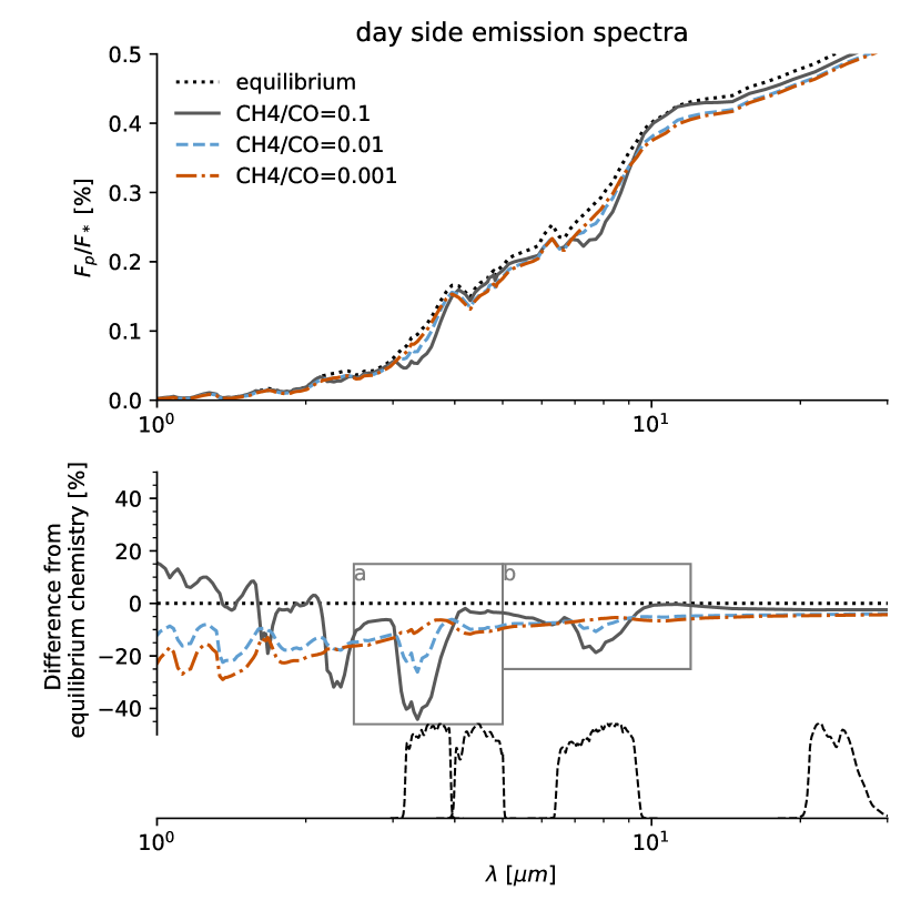
Figure 10: Predicted day side emission spectra, as would be observed at secondary eclipse. The ratio of the planet flux to the stellar flux is plotted in the top panel. The bottom panel shows the relative difference of the flux in each of the quenched simulations to the flux in the equilibrium chemistry simulation. The regions plotted in panels a and b of Fig. 12 are indicated with gray boxes. The dashed black lines at the bottom indicate the filter sensitivity profiles of the Spitzer 3.6 $\mu$m, 4.5 $\mu$m, 8 $\mu$m and 24 $\mu$m bands. The emission spectra in this Figure are available as Data behind the Figure.

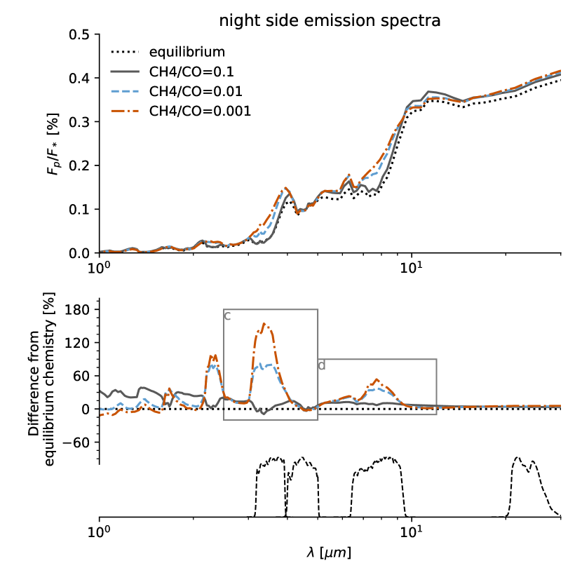
Figure 11: Same as Fig. 10 but for night side emission spectra, as would be observed right before or after transit. The emission spectra in this figure are available as Data behind the Figure.

3.6 Simulated JWST spectra

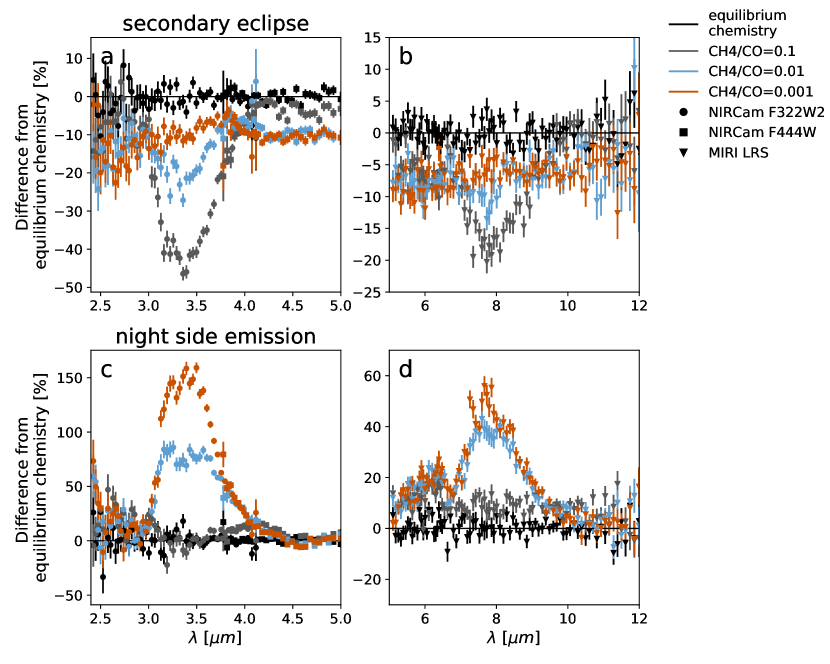
Figure 12: Simulated JWST observations for NIRCam (left panels) using the F322W2 (circles) and F444W (squares) grisms and MIRI LRS (right panels, triangles). Plotted is the difference to the flux predicted by the equilibrium chemistry model, binned to a spectral resolution of $R\approx 50$, with 1$\sigma$ error bars. The simulated observations in this figure are available as Data behind the Figure.

In order to determine whether the CH₄/CO ratio can be distinguished with future observations, we simulated JWST observations of HD 189733b using PandExo (Batalha et al., 2017). PandExo is a noise simulator that uses the Space Telescope Science Institute’s exposure time calculator, Pandeia (Pontoppidan et al., 2016). Using PandExo, we find that in many NIRSpec and NIRISS observing modes the detector becomes saturated due to HD 189733b’s brightness (J=6.07). We therefore simulate data for two of NIRCam’s grisms, F322W2 (2.413-4.083 $\mu$m) and F444W (3.835-5.084 $\mu$m), and MIRI Low-Resolution Spectroscopy (LRS) (5-12 $\mu$m). These three modes all remain below 80% full well saturation across the detector. The NIRCam grisms ultilize the 64 x 2048 pixel subarray to reduce readout times. MIRI LRS uses a dedicated slitless prism subarray region.

Each instrument mode was simulated assuming only a single eclipse with equal time in eclipse as out of eclipse. We also assume a 40 PPM noise floor, which is similar to the noise floors found in WFC3 on HST (Kreidberg et al., 2014). We simulated data for different CH₄/CO ratios and for equilibrium chemistry. Observations were simulated for both the day side and the night side. Since PandExo only models eclipses and transits and not phase curves, the planet’s night side spectrum was given to PandExo as if it were the planet’s day side since the expected noise should be the same, except for the reduced brightness of the planet’s night side. We plot the results for the CO dominated simulations in Figure 12 in terms of the difference to the equilibrium chemistry model. We also include the simulated observations for the equilibrium chemistry case to give a sense of the expected residuals. Note that the scale on the y-axis is different in each panel. For better orientation, the regions shown in each panel are indicated with grey boxes in Figures 10 and 11.

In secondary eclipse, all quenched cases can be distinguished from the disequilibrium chemistry case in all three observing modes. The different CH₄/CO ratios 0.1, 0.01 and 0.001 can also clearly be distinguished from each other. With MIRI LRS, the fluxes in the CH₄/CO=0.01 and 0.001 cases are relatively close to each other, but can still be distinguished from each other at greater than $3\sigma$ confidence.

Looking at night side emission spectra, the relative deviations from the equilibrium chemistry spectra are much larger. The CH₄/CO=0.01 and 0.001 can easily be distinguished from equilibrium chemistry in all three observing modes. The night side fluxes of the CH₄/CO=0.1 case are in general much closer to the equilibrium chemistry case in the wavelength ranges covered by these observing modes, but still can be distinguished from disequilibrium chemistry. With the NIRCam F322W2 grism and MIRI LRS, it is possible to clearly distinguish the three shown CH₄/CO ratios from each other as well. With simulated data from the NIRCam F444W grism, it is still possible to tell the different CH₄/CO ratios apart from each other at $3\sigma$ confidence, but differences between the quenched ratios are only evident at wavelengths shorter than 4 $\mu$m, at the very edge of the wavelength range of this grism. Thus, it may not be the first choice for observing disequilibrium chemistry.

Our intent in presenting these simulated observations is to demonstrate the need of including disequilibrium chemistry when interpreting future observations with JWST and to guide observers in which regions to look for signatures of disequilibrium carbon chemistry. However, it would be premature to conclude that one would be able to determine the CH₄/CO ratio, as other factors not considered in this work can influence the results of GCM simulations and the emission spectra, including clouds, metallicity, C/O ratio and atmospheric drag (see Section 4.2). Especially an optically thick cloud deck on the night side could limit our ability to observe signatures of disequilibrium chemistry, as it would block emission from the layers in the atmosphere below the cloud deck. This could mute the strongly visible CH₄ features in Figures 10 to 12 in which the difference to equilibrium chemistry is most obvious. Future work in this direction is necessary.

4 Discussion

4.1 Importance of including disequilibrium chemistry in GCM

In their study of HD 209458b, Drummond et al. (2018b) find that the effect of transport-induced disequilibrium chemistry on the temperature structure and winds is $\sim 1\%$ relative to otherwise similar models with chemical equilibrium. In contrast, in our simulations of HD 189733b we find an effect on the temperature of up to $\sim 5-10\%$ across large regions (larger changes in very localized regions) in the more likely CO-dominated regime and even larger temperature changes in the CH₄-dominated regime. While this paper was in review, Drummond et al. (2018a) found a similar result in their simulations of HD 189733b. This raises the question of why this effect is so much larger on HD 189733b. The answer lies in the cooler temperature of HD 189733b. On the hotter HD 209458b (equilibrium temperature $T_{eq}\approx 1450$ K), CO remains the dominant species even on the night side in both equilibrium and disequilibrium chemistry. The change in opacity due to disequilibrium chemistry is thus less drastic. In contrast, on the cooler HD 189733b ($T_{eq}\approx 1200$ K) the night side is cold enough that with equilibrium chemistry, CH₄ becomes the dominant species on a significant fraction of the night side. In disequilibrium chemistry, however, CO is expected to be the dominant species everywhere at pressures below 1 bar. Thus, when including disequilibrium chemistry in the radiative transfer, for most of the night side the dominant carbon species switches from CH₄ to CO, significantly changing the opacities. With this switch between CH₄ and CO as dominant species, the H₂O abundance changes by a factor of about two as well, further affecting the opacities. For planets much cooler than HD 189733b, even the day side becomes CH₄ dominated in both equilibrium and disequilibrium chemistry. Regardless of exact disequilibrium abundances, the dominant species remains the same as in equilibrium chemistry on these planets. For this situation, we would thus again expect a smaller effect on the opacities and thus on the resulting temperatures.

Therefore, we expect that including the effect of disequilibrium carbon chemistry on the opacities in the GCM is most important for planets for which equilibrium chemistry predicts a CO dominated day side but a CH₄ dominated night side. Assuming solar metallicity, the equilibrium abundance of CH₄ becomes comparable to the CO abundance on the coldest regions of the night side for planets with equilibrium temperatures below $\sim 1300$ K (Kataria et al., 2016, Fig. 7, taking the morning terminator profiles to be representative of the coldest regions of the planet). This demarcates the upper boundary of the regime in which we expect disequilibrium carbon abundances to be important in GCMs. The colder end of this regime has been less explored by GCMs. Based on 1D models, for solar composition the day side is expected to transition from CO-dominated to CH₄-dominated roughly at equilibrium temperatures around 700 K, with the transition occurring at slightly higher temperatures in equilibrium chemistry and at slightly lower temperatures in disequilibrium chemistry (Moses et al., 2013b; Venot et al., 2014; Miguel & Kaltenegger, 2014). We thus expect that it is important to include disequilibrium CH₄ and CO abundances in GCMs of hot Jupiters for planets with equilibrium temperatures between $\sim$ 600 K and 1300 K, assuming solar abundances. As the temperature of the transition between CH₄ and CO strongly depends on the metallicity and C/O ratio, this temperature range may change depending on atmospheric composition. Future work spanning a range of planets is necessary to test this prediction. This could include both simulations coupling a chemical scheme to a GCM similar to Drummond et al. (2018b) and Cooper & Showman (2006) and simulations with a simpler approach comparable to ours.

While we expect these findings to qualitatively also apply to atmospheres with moderate deviations from solar metallicity and C/O ratio, our conclusions may not apply to planets with C/O ratios $>$1. In that case, the composition changes drastically and the abundances of CH₄ and HCN can become comparable to CO for both equilibrium chemistry and disequilibrium chemistry even on the day sides of planets with temperatures comparable to HD 189733b or hotter (Moses et al., 2013a). However, up to date no planet atmosphere has been shown to have a C/O ratio$>1$ (Line et al., 2014; Benneke, 2015).

We further note that our method of assuming a constant CH₄/CO ratio is only a good approximation for situations in which CH₄ and CO abundances have been homogenized horizontally and vertically throughout most of the photosphere (at pressures between $\sim$1 mbar to 1 bar). While for hot Jupiters with relatively cool equilibrium temperatures such as HD 189733b this is expected to be the case (Cooper & Showman, 2006; Agúndez et al., 2014; Drummond et al., 2018b), there can be situations in which abundances are homogenized only horizontally but not vertically or in which the quenching happens only at lower pressures and significant parts of the photoshpere are still in chemical equilibrium (Agúndez et al., 2014; Mendonça et al., 2018a). In general, such situations are expected for planets with hotter day side temperatures and weak vertical mixing. Future work is necessary to better understand when such situations occur and to clarify the relative importance of horizontal and vertical quenching.

4.2 Other factors impacting the predicted phase curves

As discussed in Section 3.3, disequilibrium carbon chemistry barely affects the 4.5 $\mu$m phase curve while significantly decreasing the phase curve amplitude in the 3.6 $\mu$m band, thus worsening the fit of the 3.6 $\mu$m phase curve to observations. Among the simulations we ran for this paper, the equilibrium chemistry simulation actually matches the data better than any of the disequilibrium chemistry simulations. At this point, we would like to note that the equilibrium chemistry phase curve in this paper somewhat differs from the solar metallicity (equlibrium chemistry) phase curve presented in Showman et al. (2009) and Knutson et al. (2012). This is due to updates of the opacities (Freedman et al., 2014) and planetary and stellar parameters. In general, in all wavelength bands, the phase curve amplitude increases and the phase curve offset decreases slightly with the updated opacities. With these changes, the issue of the model overpredicting the night side fluxes in the 4.5 $\mu$m band is somewhat mitigated and difference in phase curve offset becomes the more dominant discrepancy between observations and the solar metallicity equilibrium chemistry model.

Our finding that the phase curve from the equilibrium chemistry simulation matches the observational phase curve better than the ones assuming disequilibrium chemistry is in agreement with Dobbs-Dixon & Cowan (2017) who find that based on their GCM the phase curve data are consistent with equilibrium chemistry. Does this mean that the atmosphere of HD 189733b is in chemical equilibrium? Based on the theoretical understanding of chemical kinetics and atmospheric dynamics, this is highly unlikely. It is much more likely that other processes that our model does not take into account are responsible for the shape of the phase curve. A likely explanation is the presence of clouds on the night side of HD 189733b. Cloud microphysics models (Lee et al., 2015; Powell et al., 2018) and GCM simulations including clouds with varying levels of complexity (e.g. Parmentier et al., 2016; Oreshenko et al., 2016; Lee et al., 2016; Lines et al., 2018) show that in the atmospheres of hot Jupiters there exist a variety of species that may condense to form clouds on the night side. An optically thick cloud deck on the night side would block the emission from hotter, deeper layers in the atmosphere, thus reducing the flux emitted on the night side over a broad range of wavelengths. Clouds present only on the night side of the planet would therefore increase the amplitude of the phase curve. Mendonça et al. (2018a) include a simple parametrization of night side clouds in their GCM simulations of WASP-43b and study the effect on the spectra and phase curves. They are able to match the spectrally resolved HST WFC3 phase curve from 1.1-1.7 $\mu$m and the Spitzer 3.6 $\mu$m phase curve quite naturally. This demonstrates both the importance of including the effect of night side clouds and the potential of clouds to explain the low observed night side fluxes on several hot Jupiters. However, the effect of clouds on spectra depends on many unknown properties such as cloud top pressure, composition and latitudinal and longitudinal distribution and more theoretical and observational work is necessary. Furthermore, to match the 4.5 $\mu$m phase curve, Mendonça et al. (2018a) include additional CO₂ compared to the equilibrium chemistry abundance on the night side. There is no clear theoretical motivation for additional CO₂ on the night side—in contrast, Agúndez et al. (2014) find that disequilibrium chemistry tends to reduce the CO₂ abundance on the night sides of HD 209458b and HD 189733b compared to equilibrium chemistry. Mendonça et al. (2018b) find that disequilibrium chemistry reduces the CO₂ abundance on the night side in the C/O=0.5 case but increases it in the C/O=2 case. They conclude that the changes in CO₂ due to disequilibrium chemistry cannot resolve the remaining discrepancy in the 4.5 $\mu$m band.

Especially on relatively cool planets such as HD 189733b, clouds need not be restricted to the night side. An optically thick cloud deck extending into parts of the day side or even covering the entire planet is another plausible possibility (e.g., Parmentier et al., 2016; Roman & Rauscher, 2019). Using a simple, constant particle size cloud scheme that includes radiative feedback, Roman & Rauscher (2019) find that their cloud distribution (covering large fractions of the day side) results in a larger phase amplitude and lower phase offset than in the cloud-free case. They stress the role of cloud radiative feedback in shaping the phase curve. However, it is likely that a realistic distribution of clouds over the planets is not uniform in particle size and density (Lee et al., 2016; Lines et al., 2018), potentially resulting in a much more complex effect on the phase curve (Lines et al., 2018).

In addition to clouds, several other parameters not explored in this study can significantly impact the phase curves, including non-solar metallicities and C/O ratios and atmospheric drag due to subgrid-scale turbulence or due to Lorentz forces in a partially ionized atmosphere. Independent of these factors, there are also moderate uncertainties associated with the numerical model, most notably the uncertainty in the opacities of some species which are not well-known at high temperatures. In this context, we would like to remind the reader that the simulations presented are pure forward models and we make no attempt to fit the observational data. The general trends observed in this paper thus are much more important and meaningful than specific predictions for the emitted flux or other observable quantities.

5 Conclusion

We have included the radiative effect of transport-induced disequilibrium CH₄, CO and H₂O abundances in a GCM to study the effect on the atmospheric structure, phase curves and emission spectra. We have assumed that the ratio of CH₄ to CO is constant throughout the entire simulation (an assumption that is expected to be well fulfilled at pressures between $\sim 10^{-4}$ bars and 1 bar) and treat the CH₄/CO ratio as free parameter. The water abundance is updated accordingly, such that the total number of oxygen atoms is preserved. It is important to include this change in the water abundance, as in equilibrium chemistry the water abundance varies by a factor of $\sim 2$ between the CO-dominated day side and the CH₄-dominated night side. Assuming vertical and horizontal quenching, however, the water abundance is expected to be homogenized between day and night side. We ran simulations of hot Jupiter HD 189733b with eight different quenched CH₄/CO ratios.

We find that in the CO dominated case, which is the case favored by chemical kinetics models, the temperature changes locally by up to 150 K, with cooler temperatures compared to equilibrium chemistry on the day side and warmer temperatures on part of the night side. In the less plausible CH₄ dominated case, the addition of greenhouse gases leads to hotter temperatures everywhere at pressures higher than a few tens of mbars. When comparing the predicted phase curves from GCM simulations including disequilibrium CH₄ and CO abundances to phase curves obtained from an equilibrium chemistry GCM simulation that has been post-processed assuming quenched CH₄/CO abundances, we find that the eastward offset of the phase curve maximum can differ by up to $10^{\circ}$.

We thus conclude that it is important to self-consistently include the effect of disequilibrium abundances of CH₄ and CO on the opacities in GCMs rather than including disequilibrium abundances only in the post-processing while continuing to use opacities based on equilibrium chemistry abundances in the GCM. This is in contrast to Drummond et al. (2018b) who find in their study of HD 209458b that the effect of radiative feedback of disequilibrium abundances on the temperature and wind fields is only $\sim 1\%$, but agrees with their more recent findings for HD 189733b (Drummond et al., 2018a). These seemingly conflicting results can be understood when considering the difference in the equilibrium temperatures of the planets: On the hotter HD 209458b, the CH₄ abundance remains low compared to the CO and H₂O abundances in both equilibrium and disequilibrium chemistry even on the night side. In contrast, on the cooler HD 189733b, the night side is cool enough to be dominated by CH₄ in equilibrium chemistry. Including disequilibrium chemistry thus changes the dominant carbon species on half of the planet, resulting in much larger changes. In addition, in the regions where disequilibrium chemistry changes the dominant carbon species, the water abundance is also altered by a factor of $\sim 2$, further contributing to the effect on temperatures.

Furthermore, we show that disequilibrium CH₄ and CO abundances have only a small effect on the Spitzer 4.5 $\mu$m phase curve despite CO having a prominent absorption band within this wavelength band. This is because the change in opacity due to CO is offset by a change in water opacity in the opposite direction. In wavelength regions dominated by CH₄ opacity, including the Spitzer 3.6 $\mu$m and 8 $\mu$m bands, the phase curve amplitude decreases significantly, resulting in a much worse fit to the observed Spitzer 3.6 $\mu$m and 8 $\mu$m phase curves. We thus conclude that disequilibrium carbon chemistry cannot explain the observed low night side fluxes in the 4.5 $\mu$m band, in contrast to the interpretation of Knutson et al. (2012). Other effects, for example night side clouds, must be responsible for the observed shape of the phase curve.

While disequilibrium chemistry does not explain existing observations of HD 189733b, it may be detectable on other hot Jupiters with a similar equilibrium temperature. Therefore, we examine the effect of disequilibrium carbon chemistry on emission spectra and simulated JWST observations. We find that in the expected CO dominated regime, spectral regions dominated by methane absorption bands are most suitable to observe disequilibrium abundances. Assuming that the spectral signatures of disequilibrium carbon chemistry are not obscured by clouds or other effects not considered in our model, it will be possible to distinguish between different quenched ratios with JWST in both secondary eclipse and phase curve observations.

References

- Adcroft et al. (2004) Adcroft, A., Campin, J.-M., Hill, C., & Marshall, J. 2004, Monthly Weather Review, 132, 2845, doi: 10.1175/MWR2823.1
- Agol et al. (2010) Agol, E., Cowan, N. B., Knutson, H. A., et al. 2010, ApJ, 721, 1861, doi: 10.1088/0004-637X/721/2/1861
- Agúndez et al. (2014) Agúndez, M., Parmentier, V., Venot, O., Hersant, F., & Selsis, F. 2014, A&A, 564, A73, doi: 10.1051/0004-6361/201322895
- Agúndez et al. (2012) Agúndez, M., Venot, O., Iro, N., et al. 2012, A&A, 548, A73, doi: 10.1051/0004-6361/201220365
- Amundsen et al. (2017) Amundsen, D. S., Tremblin, P., Manners, J., Baraffe, I., & Mayne, N. J. 2017, A&A, 598, A97, doi: 10.1051/0004-6361/201629322
- Amundsen et al. (2016) Amundsen, D. S., Mayne, N. J., Baraffe, I., et al. 2016, A&A, 595, A36, doi: 10.1051/0004-6361/201629183
- Batalha et al. (2017) Batalha, N. E., Mandell, A., Pontoppidan, K., et al. 2017, PASP, 129, 064501, doi: 10.1088/1538-3873/aa65b0
- Benneke (2015) Benneke, B. 2015, ArXiv e-prints, arXiv:1504.07655. https://arxiv.org/abs/1504.07655
- Boyajian et al. (2015) Boyajian, T., von Braun, K., Feiden, G. A., et al. 2015, MNRAS, 447, 846, doi: 10.1093/mnras/stu2502
- Burrows et al. (2003) Burrows, A., Sudarsky, D., & Hubbard, W. B. 2003, ApJ, 594, 545, doi: 10.1086/376897
- Burrows et al. (1997) Burrows, A., Marley, M., Hubbard, W. B., et al. 1997, ApJ, 491, 856, doi: 10.1086/305002
- Cooper & Showman (2006) Cooper, C. S., & Showman, A. P. 2006, ApJ, 649, 1048, doi: 10.1086/506312
- Dobbs-Dixon & Agol (2013) Dobbs-Dixon, I., & Agol, E. 2013, MNRAS, 435, 3159, doi: 10.1093/mnras/stt1509
- Dobbs-Dixon & Cowan (2017) Dobbs-Dixon, I., & Cowan, N. B. 2017, ApJ, 851, L26, doi: 10.3847/2041-8213/aa9bec
- Dobbs-Dixon & Lin (2008) Dobbs-Dixon, I., & Lin, D. N. C. 2008, ApJ, 673, 513, doi: 10.1086/523786
- Drummond et al. (2018a) Drummond, B., Mayne, N. J., Manners, J., et al. 2018a, ApJ, 869, 28, doi: 10.3847/1538-4357/aaeb28
- Drummond et al. (2016) Drummond, B., Tremblin, P., Baraffe, I., et al. 2016, A&A, 594, A69, doi: 10.1051/0004-6361/201628799
- Drummond et al. (2018b) Drummond, B., Mayne, N. J., Manners, J., et al. 2018b, ApJ, 855, L31, doi: 10.3847/2041-8213/aab209
- Fortney et al. (2006) Fortney, J. J., Cooper, C. S., Showman, A. P., Marley, M. S., & Freedman, R. S. 2006, ApJ, 652, 746, doi: 10.1086/508442
- Fortney et al. (2008) Fortney, J. J., Lodders, K., Marley, M. S., & Freedman, R. S. 2008, ApJ, 678, 1419, doi: 10.1086/528370
- Fortney et al. (2005) Fortney, J. J., Marley, M. S., Lodders, K., Saumon, D., & Freedman, R. 2005, ApJ, 627, L69, doi: 10.1086/431952
- Freedman et al. (2014) Freedman, R. S., Lustig-Yaeger, J., Fortney, J. J., et al. 2014, ApJS, 214, 25, doi: 10.1088/0067-0049/214/2/25
- Freedman et al. (2008) Freedman, R. S., Marley, M. S., & Lodders, K. 2008, ApJS, 174, 504, doi: 10.1086/521793
- Goody & Yung (1989) Goody, R. M., & Yung, Y. L. 1989, Atmospheric Radiation : Theoretical Basis (Oxford University Press)
- Guillot & Showman (2002) Guillot, T., & Showman, A. P. 2002, A&A, 385, 156, doi: 10.1051/0004-6361:20011624
- Hauschildt et al. (1999) Hauschildt, P. H., Allard, F., & Baron, E. 1999, ApJ, 512, 377, doi: 10.1086/306745
- Heng et al. (2011) Heng, K., Frierson, D. M. W., & Phillipps, P. J. 2011, MNRAS, 418, 2669, doi: 10.1111/j.1365-2966.2011.19658.x
- Kataria et al. (2014) Kataria, T., Showman, A. P., Fortney, J. J., Marley, M. S., & Freedman, R. S. 2014, ApJ, 785, 92, doi: 10.1088/0004-637X/785/2/92
- Kataria et al. (2015) Kataria, T., Showman, A. P., Fortney, J. J., et al. 2015, ApJ, 801, 86, doi: 10.1088/0004-637X/801/2/86
- Kataria et al. (2013) Kataria, T., Showman, A. P., Lewis, N. K., et al. 2013, ApJ, 767, 76, doi: 10.1088/0004-637X/767/1/76
- Kataria et al. (2016) Kataria, T., Sing, D. K., Lewis, N. K., et al. 2016, ApJ, 821, 9, doi: 10.3847/0004-637X/821/1/9
- Knutson et al. (2007) Knutson, H. A., Charbonneau, D., Allen, L. E., et al. 2007, Nature, 447, 183, doi: 10.1038/nature05782
- Knutson et al. (2009) Knutson, H. A., Charbonneau, D., Cowan, N. B., et al. 2009, ApJ, 690, 822, doi: 10.1088/0004-637X/690/1/822
- Knutson et al. (2012) Knutson, H. A., Lewis, N., Fortney, J. J., et al. 2012, ApJ, 754, 22, doi: 10.1088/0004-637X/754/1/22
- Komacek & Youdin (2017) Komacek, T. D., & Youdin, A. N. 2017, ApJ, 844, 94, doi: 10.3847/1538-4357/aa7b75
- Kreidberg et al. (2014) Kreidberg, L., Bean, J. L., Désert, J.-M., et al. 2014, Nature, 505, 69, doi: 10.1038/nature12888
- Lee et al. (2016) Lee, G., Dobbs-Dixon, I., Helling, C., Bognar, K., & Woitke, P. 2016, A&A, 594, A48, doi: 10.1051/0004-6361/201628606
- Lee et al. (2015) Lee, G., Helling, C., Dobbs-Dixon, I., & Juncher, D. 2015, A&A, 580, A12, doi: 10.1051/0004-6361/201525982
- Lewis et al. (2014) Lewis, N. K., Showman, A. P., Fortney, J. J., Knutson, H. A., & Marley, M. S. 2014, ApJ, 795, 150, doi: 10.1088/0004-637X/795/2/150
- Lewis et al. (2010) Lewis, N. K., Showman, A. P., Fortney, J. J., et al. 2010, ApJ, 720, 344, doi: 10.1088/0004-637X/720/1/344
- Line et al. (2014) Line, M. R., Knutson, H., Wolf, A. S., & Yung, Y. L. 2014, ApJ, 783, 70, doi: 10.1088/0004-637X/783/2/70
- Lines et al. (2018) Lines, S., Mayne, N. J., Boutle, I. A., et al. 2018, A&A, 615, A97, doi: 10.1051/0004-6361/201732278
- Lodders & Fegley (2002) Lodders, K., & Fegley, B. 2002, Icarus, 155, 393, doi: 10.1006/icar.2001.6740
- Marley & McKay (1999) Marley, M. S., & McKay, C. P. 1999, Icarus, 138, 268, doi: 10.1006/icar.1998.6071
- Marley et al. (1996) Marley, M. S., Saumon, D., Guillot, T., et al. 1996, Science, 272, 1919, doi: 10.1126/science.272.5270.1919
- Marley et al. (2002) Marley, M. S., Seager, S., Saumon, D., et al. 2002, ApJ, 568, 335, doi: 10.1086/338800
- Mayne et al. (2014) Mayne, N. J., Baraffe, I., Acreman, D. M., et al. 2014, A&A, 561, doi: 10.1051/0004-6361/201322174
- McKay et al. (1989) McKay, C. P., Pollack, J. B., & Courtin, R. 1989, Icarus, 80, 23, doi: 10.1016/0019-1035(89)90160-7
- Mendonça et al. (2016) Mendonça, J. M., Grimm, S. L., Grosheintz, L., & Heng, K. 2016, ApJ, 829, 115, doi: 10.3847/0004-637X/829/2/115
- Mendonça et al. (2018a) Mendonça, J. M., Malik, M., Demory, B.-O., & Heng, K. 2018a, AJ, 155, 150, doi: 10.3847/1538-3881/aaaebc
- Mendonça et al. (2018b) Mendonça, J. M., Tsai, S.-m., Malik, M., Grimm, S. L., & Heng, K. 2018b, ApJ, 869, 107, doi: 10.3847/1538-4357/aaed23
- Menou (2019) Menou, K. 2019, MNRAS, 485, L98, doi: 10.1093/mnrasl/slz041
- Miguel & Kaltenegger (2014) Miguel, Y., & Kaltenegger, L. 2014, ApJ, 780, 166, doi: 10.1088/0004-637X/780/2/166
- Moses et al. (2013a) Moses, J. I., Madhusudhan, N., Visscher, C., & Freedman, R. S. 2013a, ApJ, 763, 25, doi: 10.1088/0004-637X/763/1/25
- Moses et al. (2011) Moses, J. I., Visscher, C., Fortney, J. J., et al. 2011, ApJ, 737, 15, doi: 10.1088/0004-637X/737/1/15
- Moses et al. (2013b) Moses, J. I., Line, M. R., Visscher, C., et al. 2013b, ApJ, 777, 34, doi: 10.1088/0004-637X/777/1/34
- Oreshenko et al. (2016) Oreshenko, M., Heng, K., & Demory, B.-O. 2016, MNRAS, 457, 3420, doi: 10.1093/mnras/stw133
- Parmentier et al. (2016) Parmentier, V., Fortney, J. J., Showman, A. P., Morley, C., & Marley, M. S. 2016, ApJ, 828, 22, doi: 10.3847/0004-637X/828/1/22
- Parmentier et al. (2013) Parmentier, V., Showman, A. P., & Lian, Y. 2013, A&A, 558, A91, doi: 10.1051/0004-6361/201321132
- Parmentier et al. (2018) Parmentier, V., Line, M. R., Bean, J. L., et al. 2018, A&A, 617, A110, doi: 10.1051/0004-6361/201833059
- Perna et al. (2012) Perna, R., Heng, K., & Pont, F. 2012, ApJ, 751, 59, doi: 10.1088/0004-637X/751/1/59
- Pontoppidan et al. (2016) Pontoppidan, K. M., Pickering, T. E., Laidler, V. G., et al. 2016, in Proc. SPIE, Vol. 9910, Observatory Operations: Strategies, Processes, and Systems VI, 991016
- Powell et al. (2018) Powell, D., Zhang, X., Gao, P., & Parmentier, V. 2018, ApJ, 860, 18, doi: 10.3847/1538-4357/aac215
- Rauscher & Menou (2012) Rauscher, E., & Menou, K. 2012, ApJ, 750, 96, doi: 10.1088/0004-637X/750/2/96
- Roman & Rauscher (2019) Roman, M., & Rauscher, E. 2019, ApJ, 872, 1, doi: 10.3847/1538-4357/aafdb5
- Shapiro (1970) Shapiro, R. 1970, Reviews of Geophysics and Space Physics, 8, 359, doi: 10.1029/RG008i002p00359
- Sharp & Burrows (2007) Sharp, C. M., & Burrows, A. 2007, ApJS, 168, 140, doi: 10.1086/508708
- Showman et al. (2013) Showman, A. P., Fortney, J. J., Lewis, N. K., & Shabram, M. 2013, ApJ, 762, 24, doi: 10.1088/0004-637X/762/1/24
- Showman et al. (2009) Showman, A. P., Fortney, J. J., Lian, Y., et al. 2009, ApJ, 699, 564, doi: 10.1088/0004-637X/699/1/564
- Showman & Guillot (2002) Showman, A. P., & Guillot, T. 2002, A&A, 385, 166, doi: 10.1051/0004-6361:20020101
- Showman et al. (2015) Showman, A. P., Lewis, N. K., & Fortney, J. J. 2015, ApJ, 801, 95, doi: 10.1088/0004-637X/801/2/95
- Showman & Polvani (2011) Showman, A. P., & Polvani, L. M. 2011, ApJ, 738, doi: 10.1088/0004-637X/738/1/71
- Stevenson et al. (2017) Stevenson, K. B., Line, M. R., Bean, J. L., et al. 2017, AJ, 153, 68, doi: 10.3847/1538-3881/153/2/68
- Thrastarson & Cho (2011) Thrastarson, H. T., & Cho, J. Y.-K. 2011, ApJ, 729, 117, doi: 10.1088/0004-637X/729/2/117
- Toon et al. (1989) Toon, O. B., McKay, C. P., Ackerman, T. P., & Santhanam, K. 1989, J. Geophys. Res., 94, 16287, doi: 10.1029/JD094iD13p16287
- Tremblin et al. (2017) Tremblin, P., Chabrier, G., Mayne, N. J., et al. 2017, ApJ, 841, 30, doi: 10.3847/1538-4357/aa6e57
- Tsai et al. (2018) Tsai, S.-M., Kitzmann, D., Lyons, J. R., et al. 2018, ApJ, 862, 31, doi: 10.3847/1538-4357/aac834
- Venot et al. (2014) Venot, O., Agúndez, M., Selsis, F., Tessenyi, M., & Iro, N. 2014, A&A, 562, A51, doi: 10.1051/0004-6361/201322485
- Visscher et al. (2006) Visscher, C., Lodders, K., & Fegley, Jr., B. 2006, ApJ, 648, 1181, doi: 10.1086/506245
- Visscher & Moses (2011) Visscher, C., & Moses, J. I. 2011, ApJ, 738, 72, doi: 10.1088/0004-637X/738/1/72
- Zellem et al. (2014) Zellem, R. T., Lewis, N. K., Knutson, H. A., et al. 2014, ApJ, 790, 53, doi: 10.1088/0004-637X/790/1/53