MCRM: Mother Compact Recurrent Memory

Abstract

LSTMs and GRUs are the most common recurrent neural network architectures used to solve temporal sequence problems. The two architectures have differing data flows dealing with a common component called the cell state (also referred to as the memory). We attempt to enhance the memory by presenting a modification that we call the Mother Compact Recurrent Memory (MCRM). MCRMs are a type of a nested LSTM-GRU architecture where the cell state is the GRU hidden state. The concatenation of the forget gate and input gate interactions from the LSTM are considered an input to the GRU cell. Because MCRMs has this type of nesting, MCRMs have a compact memory pattern consisting of neurons that acts explicitly in both long-term and short-term fashions. For some specific tasks, empirical results show that MCRMs outperform previously used architectures.

1 Introduction

Recurrent neural networks (RNNs) are a class of neural networks that can relate temporal information. They have been widely used for a lot of problems including image caption generation (?; ?; ?; ?), text to speech generation (?; ?; ?), object detection and tracking (?; ?; ?; ?; ?; ?), neural machine translation (?; ?; ?; ?; ?). RNNs are generally categorized into three well-known architectures, Vanilla RNNs, Long short-term memory (LSTM) proposed by (?) and Gated recurrent neural networks (GRU) proposed by (?). The vanishing and exploding gradients are well-known Vanilla RNNs problems, which GRUs and LSTMs solves. Vanilla RNNs also lack the ability to remember long-term sequences, unlike GRUs and LSTMs. The main difference between LSTMs and GRUs are in the terms of architecture. LSTMs have more control gates than GRUs do. LSTM output is a part of the cell state content unlike GRUs which its cell state is the output. Another difference is that GRUs are clearly computationally inexpensive, unlike LSTMs. Still there is no clear evidence that GRUs is better than LSTMs or not, see for instance the work of (?).

The core idea of LSTMs and GRUs is to control information flow to the cell state, which can be described as the memory, through control gates. Yet the cell state is very simple neural network layer. The core idea of the article is to investigate if the the performance of LSTMs or GRUs can be enhanced by developing a better cell state architecture. We noticed that Nested LSTMs (NLSTM) introduced by (?) outperforms previous RNN architectures, nonetheless the inner LSTM isn’t fully utilized as the cell state is exposed to the outer NLSTM via the output gate. Thus we chose to create a new deep recurrent model that has a GRU unit nested within a LSTM. The GRU is chosen to be inside the LSTM as it fully exposes the hidden state. The GRU represents the cell state of the LSTM. We call this architecture Mother Compact Recurrent Memory (MCRM). The Mother term came from our visualization of the LSTM as a mother that carries the GRU as a fetus. The compact term came from the compact memory pattern that is produced by MCRM which inherits both GRU and LSTM memory behaviors.

The MCRMs are positioned as follow:

1. A novel class of nested RNNs.

2. A compact memory pattern that support both long and short terms behaviors.

3. The model is validated using empirical test problems.
   

The rest of this article is organized as follows. Section 2 reviews the history of RNNs, LSTMs and GRUs and their development highlighting similar approaches. Section 3 discusses the MCRM model in details, and provides its mathematical model. An experimental validation of MCRM against different recurrent architectures on well-known benchmark recurrent tasks is shown in 4. Section 5 shows a visualization of MCRM hidden state and compares these with other RNNs cell states. This demonstrates the compact memory pattern outlined earlier. The MCRM source code is available at: https://github.com/abduallahmohamed/MCRM.

2 Related Work

One of the earliest work in the history of RNNs was by (?), this work represented an early concept of state in neural networks. It described a recurrent connection with an in-unit loop. It successfully integrated a time series data into a neural network. A simpler RNN architecture was proposed by (?) which can be called the Vanilla RNN. It simplified the concept of (?) to use a context unit or what can be called a hidden unit removing the in-unit loop that that was previously introduced. The work done by (?) provides more details about the history of RNNs and its development until it was formalized into the LSTM architecture. Different attempts to improve RNNs itself have been made, including the introduction of an auxiliary memory to enhance its performance (?). (?) introduced a gated feedback RNN architecture which stacks multiple RNNs to pass/not pass and control signals flowing from upper layers to the lower layers. Another modification for RNNs is the Clockwork RNN (?) which introduced a method that makes RNNs work for long-term sequences requirements. It was shown to outperform LSTMs and RNNs in some specific tasks.

LSTMs have been originally developed by (?). The main motivation of LSTMs is to skive the problem of vanishing gradients in vanilla RNNs and to remember longer sequences. The hidden layer of a RNN was replaced by a memory unit or what called a memory cell. The LSTM has specific function gates to control the flow of data and its storage within the memory cell. One extra gate added to the LSTM called the forget gate it has been introduced by (?) to give LSTM the ability to forget specific information from the memory cell. From this point, multiple developments has been done to improve the performance of LSTMs. One of them is to replace the feed forward units with a convolutional neural networks (CNNs) introduced by (?) to improve its ability for visual sequence problems (?). Other approaches involved stacking LSTMs (?; ?; ?) Or by introducing a depth gate between stacked LSTMs (?). Also, some proposed a hyper-architecture between RNNs and LSTMs such as the work of (?). Nesting the LSTM within another LSTM, resulting in a nested LSTM (NLSTM) is the focus of (?), which is used as a reference in this article. (?) organized LSTM in the form of a multidimensional grid. An extensive work by (?) explored different variations of LSTM by introducing six variants to the architecture. It concluded that the current LSTM is indeed performing well compared to these variants. Also it found that the forget gate and output gate activation functions are very critical to the LSTM performance.

The GRUs architecture, which is on the par with LSTMs in terms of performance, was introduced by introduced by (?). GRUs requires less memory and computationally less expensive than LSTM. GRUs in some cases may outperform LSTMs, as shown in the comparative study by (?). Also, GRUs fully expose the hidden state content unlike LSTMs. For the development of GRUs, an approach in the work done by (?) introduced the shuttleNet concept. The shuttleNet uses multiple GRUs treated as processors. These processors are loops connected to mimic the human’s brain feedback and feed-forward connections. A study on three different variants of GRUs was done by (?) concluded that the current GRUs have a similar performance as these three variants.

3 Mother Compact Recurrent Memory (MCRM)

In this section, we first define the notations used in this article. We then recall the LSTM and GRU models, and use them to derive the MCRM model.

Mathematical notions

The following mathematical notations will be used. $t$ stands for current time step, $\odot$ is the Hadamard product, $\sigma$ is the sigmoid activation function and $\tanh$ is the tanh activation function. $\mathbin{{+}\mspace{-8.0mu}{+}}$ is the concatenation symbol defined in (?). The input to any architecture is $\mathbf{x}_{t}\in\mathbb{R}^{m}$. Weights which interacts with the input are $W_{x\alpha}\in\mathbb{R}^{m\times p}$. Weights which interacts with the hidden state $\mathbf{h}_{t}\in\mathbb{R}^{p}$ are $W_{h\alpha}\in\mathbb{R}^{p\times p}$. $b_{\alpha}\in\mathbb{R}^{p}$ are the biases. $\alpha\in\{\mathbf{i},\mathbf{f},\mathbf{c},\mathbf{o},\mathbf{h},\mathbf{r},\mathbf{z},\mathbf{n}\}$ represent the different gates in both LSTM and GRU equations (LABEL:lstmeqn) ,(LABEL:gruqen) respectively.

LSTMs architecture

LSTMs address the vanishing gradient problem commonly found in RNNs by controlling the information flow through specific functions gates (?). At each time step, an LSTM maintains a hidden state vector $\mathbf{h}_{t}$ and a memory state vector $\mathbf{c}_{t}$ responsible for controlling the state updates and generating the outputs. The computation at time step $t$ is defined as follows:

$$\begin{split}&\mathbf{i}_{t}=\sigma(\mathbf{x}_{t}*W_{xi}+\mathbf{h}_{t-1}*W_{hi}+b_{i})\\ &\mathbf{f}_{t}=\sigma(\mathbf{x}_{t}*W_{xf}+\mathbf{h}_{t-1}*W_{hf}+b_{f})\\ &\mathbf{c}_{t}=\mathbf{f}_{t}\odot\mathbf{c}_{t-1}+\mathbf{i}_{t}\odot\tanh(\mathbf{x}_{t}*W_{xc}+\mathbf{h}_{t-1}*W_{hc}+b_{c})\\ &\mathbf{o}_{t}=\sigma(\mathbf{x}_{t}*W_{xo}+\mathbf{h}_{t-1}*W_{ho}+b_{o})\\ &\mathbf{h}_{t}=o_{t}\odot\tanh(c_{t})\end{split}$$ (1)

$\mathbf{c}_{t}$ is usually refereed as the cell or the memory state where the information are stored. The hidden state $\mathbf{h}_{t}$ is the output or the exposed state of an LSTM. The LSTM operation is as follows: the input gate $\mathbf{i}_{t}$ at time step $t$ decides how much information to take from the input $\mathbf{x}_{t}$ into the memory. The forget gate $\mathbf{f}_{t}$ decides how much information to keep from the previous cell state $\mathbf{c}_{t-1}$. Both input gate interaction and forget gate interaction are used to compute the new cell state $\mathbf{c}_{t}$. Then the output gate $\mathbf{o}_{t}$ is used to compute the quantity of information to expose from the cell state $\mathbf{c}_{t}$ to outside world through the hidden state $\mathbf{h}_{t}$ representing the output of LSTM.

GRUs architecture

GRUs also address the same problems found in RNNs. They have been introduced by (?). The main difference between GRUs and LSTMs is that GRUs totally expose the hidden state information through $\mathbf{h}_{t}$. They require less memory and are computationally less expensive unlike LSTMs. The computation at time step $t$ is defined as follows:

$$\begin{split}&\mathbf{r}_{t}=\sigma(W_{ir}*\mathbf{x}_{t}+b_{ir}+W_{hr}*\mathbf{h}_{t-1}+b_{hr})\\ &\mathbf{z}_{t}=\sigma(W_{iz}*\mathbf{x}_{t}+b_{iz}+W_{hz}*\mathbf{h}_{t-1}+b_{hz})\\ &\mathbf{n}_{t}=\tanh(W_{in}*\mathbf{x}_{t}+b_{in}+\mathbf{r}_{t}\odot(W_{hn}*\mathbf{h}_{t-1}+b_{hn}))\\ &\mathbf{h}_{t}=(1-\mathbf{z}_{t})\odot\mathbf{h}_{t-1}+\mathbf{z}_{t}\odot\mathbf{n}_{t}\end{split}$$ (2)

The GRU operates as follows: the reset gate $\mathbf{r}_{t}$ is used to compute how much information to remove from the previous hidden state $\mathbf{h}_{t-1}$. This reset gate interaction is added to the input $\mathbf{x}_{t}$ and saved into an intermediate vessel called the node state $\mathbf{n}_{t}$. The update gate $\mathbf{z}_{t}$ decides how much information from the previous hidden state $\mathbf{h}_{t-1}$ should be added to the node state $\mathbf{n}_{t}$ to form the new hidden state $\mathbf{h}_{t}$. This new hidden state $\mathbf{h}_{t}$ is the output of the GRU cell.

MCRMs architecture

MCRM nests a GRU cell inside an LSTM treating the GRU hidden state $\mathbf{h}_{t}^{GRU}$ as the LSTM cell state $\mathbf{c}_{t}$ . The input to the GRU unit is $\mathbf{x}_{t}^{GRU}$ which is the concatenation of what the LSTM should forget and what it should remember from the input coming into the MCRM cell, it’s defined in equation (3).

$$\begin{split}&\mathbf{x}_{t}^{GRU}=\mathbin{{+}\mspace{-8.0mu}{+}}(\mathbf{f}_{t}\odot\mathbf{c}_{t-1},\\ &\mathbf{i}_{t}\odot\tanh(\mathbf{x}_{t}*W_{xc}+\mathbf{h}_{t-1}*W_{hc}+b_{c}))\end{split}$$ (3)

The modified equation of the LSTM cell now become:

$$\begin{split}&\mathbf{i}_{t}=\sigma(\mathbf{x}_{t}*W_{xi}+\mathbf{h}_{t-1}*W_{hi}+b_{i})\\ &\mathbf{f}_{t}=\sigma(\mathbf{x}_{t}*W_{xf}+\mathbf{h}_{t-1}*W_{hf}+b_{f})\\ &\mathbf{c}_{t}=\mathbf{h}_{t}^{GRU}\\ &\mathbf{o}_{t}=\sigma(\mathbf{x}_{t}*W_{xo}+\mathbf{h}_{t-1}*W_{ho}+b_{o})\\ &\mathbf{h}_{t}=o_{t}\odot\tanh(c_{t})\end{split}$$ (4)

And the modified equations of GRU cell now becomes:

$$\begin{split}&\mathbf{r}_{t}=\sigma(W_{ir}*\mathbf{x}_{t}^{GRU}+b_{ir}+W_{hr}*\mathbf{h}_{t-1}^{GRU}+b_{hr})\\ &\mathbf{z}_{t}=\sigma(W_{iz}*\mathbf{x}_{t}^{GRU}+b_{iz}+W_{hz}*\mathbf{h}_{t-1}^{GRU}+b_{hz})\\ &\mathbf{n}_{t}=\tanh(W_{in}*\mathbf{x}_{t}^{GRU}+b_{in}+\mathbf{r}_{t}\odot(W_{hn}*\mathbf{h}_{t-1}^{GRU}+b_{hn}))\\ &\mathbf{h}_{t}^{GRU}=(1-\mathbf{z}_{t})\odot\mathbf{h}_{t-1}^{GRU}+\mathbf{z}_{t}\odot\mathbf{n}_{t}\end{split}$$ (5)

Figure 1 illustrates the data flow inside the MCRM, following equations 4 and 5. The closest architecture to MCRMs is the Nested LSTMs (NLSTMs) introduced by (?), which nests am LSTM inside another LSTM. MCRMs had the following advantages over NLSTMs: first, they are less computationally expensive than NLSTMs as they use GRUs instead of LSTM as the cell state. Secondly, they have a better neurons utilization as the full hidden state is exposed from the GRU to the LSTM unlike NLSTMs where the inner LSTM are not fully utilized because of the usage of the cell state only.

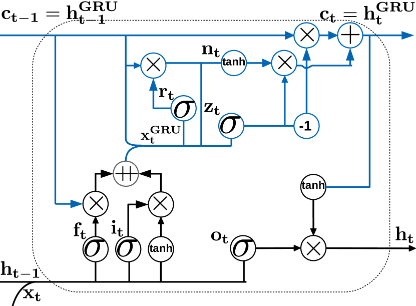
Figure 1: MCRM detailed data flow diagram starting from the previous hidden state to the next hidden state. The black colored lines refers to the LSTM part and the blue colored lines refers to the GRU part.

4 Experiments and results

In this section, the MCRM performance is evaluated empirically against different recurrent architectures on well-known tasks. For fairness of comparison, we use the same hyper-parameters as in (?). Also, our results are consist with the results from (?). These experiments were executed under a controlled environment, using the same initial random seed and weights initializations. The parameters of the models were kept the same between multiple experiments to check which architecture has a better usage of the neurons. The different configuration parameters are shown in table 2. Each experiment was executed multiple times with different initial seeds and the reported performance metrics are the mean performance of these multiple executions. We avoided the usage of any drop-out or batch normalization layers to have a fair evaluation of the performance.

Table 1: Evaluation of MCRM versus different recurrent architectures on synthetic stress tests, character-level language modeling, and word-level language modeling. The MCRM architecture outperforms most of these recurrent networks in some cases or tend to be better than other architectures across different tasks and datasets. $\ {}^{h}$ means that higher is better. ^ℓ means that lower is better.

Sequence Modeling Task	Model Size ($\approx$)	Models
		RNN	GRU	LSTM	NSLTM	MCRM
Seq. MNIST (accuracyh)	152K	19.57	98.58	85.16	91.02	98.79
Adding problem (lossℓ)	95K	0.165	3.2e-04	0.001	0.004	4.0e-06
Copy memory (loss)	3.3M	0.021	0.013	0.004	7.3e-05	8.5e-06
Char-level PTB (bpcℓ)	17.1M	1.683	1.397	1.374	1.365	1.331
Word-level PTB (pplℓ)	1.3M	140.58	110.6	110.64	140.1	120.9

The adding problem

The adding problem has been used as a stress test for sequence models. It was introduced by (?). The test is about creating an input with a length $T$ sequence of depth 2. The first dimension is randomly chosen between 0 and 1. The second dimension is all zeros except the last two elements marked by 1. The objective is find the sum the last two random elements marked by 1 in the second dimension. We used a sequence of length $T=200$. The test results are shown in table 1. MCRM outperforms all other models with an error of $4e-06$. Also, the GRU has a close performance of an error of $3.2e-04$ which explains why the MCRM have this performance. The learning curves are shown in figure 2.

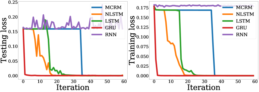
Figure 2: The loss as a function of iteration for the adding problem test predictions for both train and test datasets.

Copy memory test

This method has been used previously in (?; ?; ?) for measuring the performance of a recurrent architecture in the context of remembering information seen $T$ time steps earlier. The input sequence is in the length of $T+20$. The input sequence defined as: $\{\beta_{0},\dots,\beta_{9},\kappa_{0},\dots,\kappa_{n},\delta_{\text{delm}},\delta_{0},\dots,\delta_{9}\}$, where $\kappa$ is chosen to be a zero digit and $n=T-1$. The $\beta$ is randomly chosen from digits $\{1,\dots,8\}$. The $\delta$ is set to be digit 9, where $\delta_{\text{delm}}$ is the delimiter. The model is expected to generate an output identical to the input sequence is. A test was conducted with a sequence length of $T=1000$. The results are shown in table 1. The MCRM outperforms all other models with an error of $8.5e-06$. The learning curves are shown in figure 3.

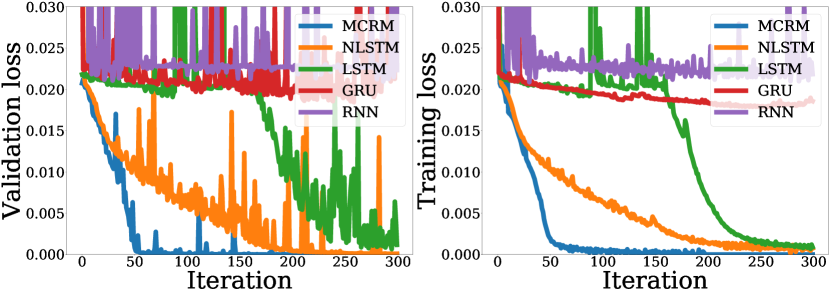
Figure 3: The loss as a function of iteration for the copy memory test predictions for both train and test datasets.

Sequential MNIST test

This test is similar in intent to the copy memory test. In this task the MNIST dataset (?) images are presented to the model as a $784\times 1$ input sequence of pixels intensity values. The recurrent model should be able to reconstruct the image again. This test was used as a stress test in several recurrent related problems (?; ?). From table 1 MCRM achieved accuracy of 98.79% outperforming any other model. Surprisingly, the LSTM and NSLTM had a poor performance unlike the GRU. We relate the success of MCRM in this task to the GRU core inside it. The learning curves are presented in figure 4.

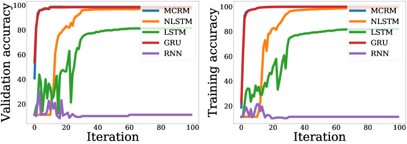
Figure 4: The accuracy as a function of iteration for the sequential MNIST predictions for both train and test datasets.

PennTreebank character and word levels tests

The PennTreebank (PTB) (?) is a text data set for both character-level and word-level language modeling tasks. It is widely used in many RNN architectures for evaluating the model performance. The PTB is divided into train, test and validation datasets. To measure the character-level task performance the bits per character (bpc) is used as a performance index. BPC has been introduced by (?)and it is defined as the cross-entropy loss (?) divided by $log\text{ 2}$. The performance index for the word-level language modeling task is the perplexity (ppl). The ppl is defined as the exponential of the cross-entropy loss. The two tasks results are reported in table 1. The reported values are from the validation dataset. When the PTB is used as character-level language corpus the MCRM outperforms other models with a bpc of 1.331 exceeding the NLSTM by 0.034 ppl. The learning curves are shown in figure 5. When the PTB used as word-level language corpus MCRM performance is in-between the GRU and NLSTM. The learning curves are shown in figure 6

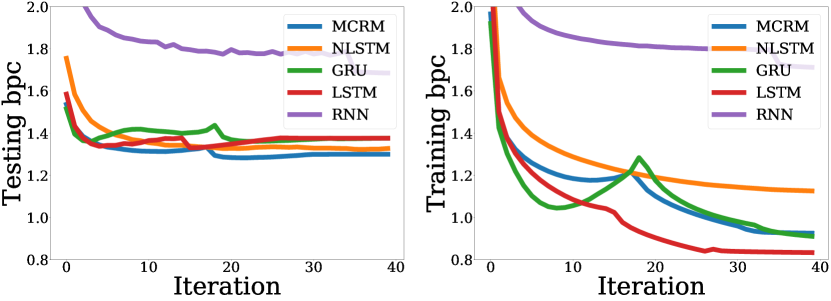
Figure 5: The bpc performance index as a function of iteration for character-level prediction on PTB’s train and test data sets.

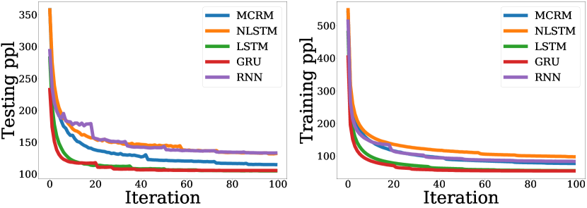
Figure 6: The ppl performance index as a function of iteration for word-level prediction on PTB’s train and test data sets.

Table 2: Parameter settings for experiments in Section 4. The integers beneath each architecture type are the hidden state sizes. ${lr}$ stands for learning rate. ${gc}$ stands for gradient clipping

Key Parameters
Dataset/Task	RNN	GRU	LSTM	NLSTM	MCRM	${lr}$, ${gc}$	Note
Adding	308	177	153	77	85	Adam ${lr}$(1e-3), ${gc}$(0.5)	NLSTM ${lr}$(0.01), ${gc}$(0.1)
Seq. MNIST	384	222	192	108	97	RMSprop ${lr}$(1e-3), ${gc}$(1.0)	NLSTM ${gc}$(0.25), LSTM ${lr}$(1e-4)
Copy Memory	1800	1050	900	448	500	RMSprop ${lr}$(5e-4), ${gc}$(1.0)	NLSTM ${lr}$(1e-4), ${gc}$(0.25)
Word-level PTB	125	119	117	100	109	SGD ${lr}$(30), ${gc}$(0.35)	-
Char-level PTB	2900	1680	1050	920	1000	Adam ${lr}$(1e-3), ${gc}$(0.15)	-

5 Visualization

To understand the internal behavior of MCRM, we performed a visual analysis of the memory cell. Following a similar approach as the work of (?), specific neurons of interest are monitored versus an input sequence. The work of (?) is also expanded by introducing a method of selecting these neurons. This method consists of a heat map of the propagation of all neurons activation values in the memory in contrast to an input sequence (shown in figure 7.). MCRM, NLSTM, LSTM and GRU are trained over the PTB character dataset, fixing the memory cell size to be around 150 neurons.

In figure 7 the heat maps columns represents a step in this visual analysis. LSTM cell states tend to have neurons changing slowly over the sequence. This is in contrast to GRU architectures where-in neuron activation values change rapidly. NLSTM outer cell acts in a short-term fashion remembering small sequences. The inner cell of the NLSTM acts in a long-term fashion to support longer sequences. MCRM memory cell has some neurons acting in an explicit long-term fashion and some acting in a short-term explicit fashion. This means by nature MCRM inherits both LSTM and GRU behaviors in a one memory cell. This leads to a better neurons utilization which is an important advantage of MCRM. The neurons of interest column in Figure 7 shows specific neurons extracted from the heat maps column that have long or short-term behaviors support the analysis of the heat maps.

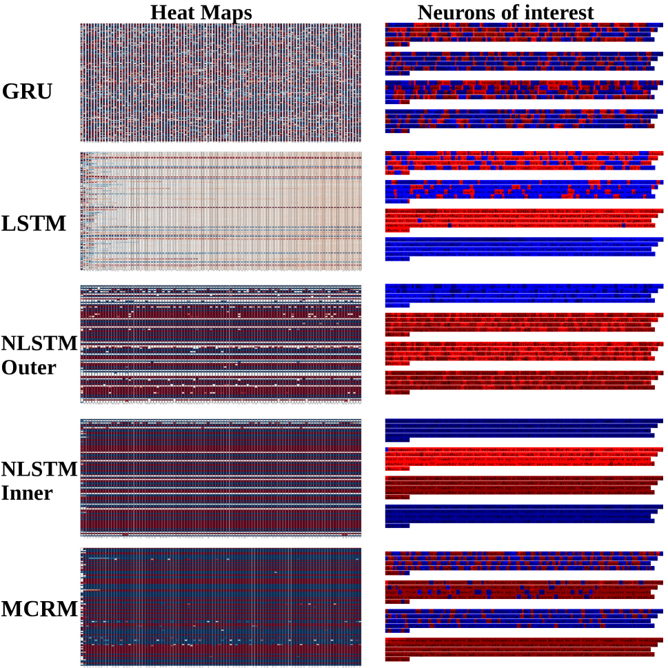
Figure 7: Heat Maps column is the heat maps of the propagation of all memory states neurons versus sequence of character inputs. The vertical axis represents neurons activation values versus the horizontal axis. The horizontal axis represents the characters input to the cell. Each row is the propagation of a specific neuron activation values.The propagation is from left to right. The neurons of interest columns is a visualization of specific neurons of interest activation values versus an input sequence of characters. Red denotes a negative cell state value, and blue a positive one. A darker shade denotes a larger magnitude. The memory state of GRU is its hidden cell state $h_{t}$. The memory state of LSTM is its cell state $C_{t}$. The memory state of NLSTM are its outer $C_{t}^{outer}$ and inner $tanh(C_{t}^{inner})$ cell states respectively. The memory state of MCRM cell is its cell state $h_{t}^{GRU}$.

6 Conclusion

Mother Compact Recurrent Memory (MCRMs) are a Nested LSTM-GRU architecture. They create a unique compact memory pattern that supports both long and short-terms behaviors. MCRMs can outperform other RNNs architectures, on benchmark tests. Because of their promising results, MCRMs could be used in temporal sequence modeling tasks.

References

- [Arik et al. 2017] Arik, S. O.; Chrzanowski, M.; Coates, A.; Diamos, G.; Gibiansky, A.; Kang, Y.; Li, X.; Miller, J.; Ng, A.; Raiman, J.; et al. 2017. Deep voice: Real-time neural text-to-speech. arXiv preprint arXiv:1702.07825.
- [Arjovsky, Shah, and Bengio 2015] Arjovsky, M.; Shah, A.; and Bengio, Y. 2015. Unitary evolution recurrent neural networks. CoRR abs/1511.06464.
- [Bahdanau, Cho, and Bengio 2014] Bahdanau, D.; Cho, K.; and Bengio, Y. 2014. Neural machine translation by jointly learning to align and translate. arXiv preprint arXiv:1409.0473.
- [Bai, Kolter, and Koltun 2018] Bai, S.; Kolter, J. Z.; and Koltun, V. 2018. An empirical evaluation of generic convolutional and recurrent networks for sequence modeling. arXiv preprint arXiv:1803.01271.
- [Cho et al. 2014] Cho, K.; van Merrienboer, B.; Gülçehre, Ç.; Bougares, F.; Schwenk, H.; and Bengio, Y. 2014. Learning phrase representations using RNN encoder-decoder for statistical machine translation. CoRR abs/1406.1078.
- [Chung et al. 2014] Chung, J.; Gülçehre, Ç.; Cho, K.; and Bengio, Y. 2014. Empirical evaluation of gated recurrent neural networks on sequence modeling. CoRR abs/1412.3555.
- [Chung et al. 2015] Chung, J.; Gulcehre, C.; Cho, K.; and Bengio, Y. 2015. Gated feedback recurrent neural networks. In International Conference on Machine Learning, 2067–2075.
- [Dey and Salem 2017] Dey, R., and Salem, F. M. 2017. Gate-variants of gated recurrent unit (gru) neural networks. arXiv preprint arXiv.
- [Donahue et al. 2015] Donahue, J.; Anne Hendricks, L.; Guadarrama, S.; Rohrbach, M.; Venugopalan, S.; Saenko, K.; and Darrell, T. 2015. Long-term recurrent convolutional networks for visual recognition and description. In Proceedings of the IEEE conference on computer vision and pattern recognition, 2625–2634.
- [Elman 1990] Elman, J. L. 1990. Finding structure in time. Cognitive science 14(2):179–211.
- [Fan et al. 2014] Fan, Y.; Qian, Y.; Xie, F.-L.; and Soong, F. K. 2014. Tts synthesis with bidirectional lstm based recurrent neural networks. In Fifteenth Annual Conference of the International Speech Communication Association.
- [Gers, Schmidhuber, and Cummins 1999] Gers, F. A.; Schmidhuber, J.; and Cummins, F. 1999. Learning to forget: Continual prediction with lstm.
- [Goodfellow, Bengio, and Courville 2016] Goodfellow, I.; Bengio, Y.; and Courville, A. 2016. Deep Learning. MIT Press. http://www.deeplearningbook.org.
- [Graves, Mohamed, and Hinton 2013] Graves, A.; Mohamed, A.; and Hinton, G. E. 2013. Speech recognition with deep recurrent neural networks. CoRR abs/1303.5778.
- [Graves 2012] Graves, A. 2012. Supervised sequence labelling. In Supervised sequence labelling with recurrent neural networks. Springer. 5–13.
- [Graves 2013] Graves, A. 2013. Generating sequences with recurrent neural networks. CoRR abs/1308.0850.
- [Greff et al. 2017] Greff, K.; Srivastava, R. K.; Koutník, J.; Steunebrink, B. R.; and Schmidhuber, J. 2017. Lstm: A search space odyssey. IEEE transactions on neural networks and learning systems 28(10):2222–2232.
- [Hochreiter and Schmidhuber 1997] Hochreiter, S., and Schmidhuber, J. 1997. Long short-term memory. Neural computation 9(8):1735–1780.
- [Jing et al. 2016] Jing, L.; Shen, Y.; Dubcek, T.; Peurifoy, J.; Skirlo, S. A.; Tegmark, M.; and Soljacic, M. 2016. Tunable efficient unitary neural networks (EUNN) and their application to RNN. CoRR abs/1612.05231.
- [Jordan 1997] Jordan, M. I. 1997. Serial order: A parallel distributed processing approach. In Advances in psychology, volume 121. Elsevier. 471–495.
- [Kalchbrenner, Danihelka, and Graves 2015] Kalchbrenner, N.; Danihelka, I.; and Graves, A. 2015. Grid long short-term memory. CoRR abs/1507.01526.
- [Kang et al. 2017] Kang, K.; Li, H.; Xiao, T.; Ouyang, W.; Yan, J.; Liu, X.; and Wang, X. 2017. Object detection in videos with tubelet proposal networks. In Proc. CVPR, volume 2, 7.
- [Karpathy and Fei-Fei 2015] Karpathy, A., and Fei-Fei, L. 2015. Deep visual-semantic alignments for generating image descriptions. In Proceedings of the IEEE conference on computer vision and pattern recognition, 3128–3137.
- [Karpathy, Johnson, and Li 2015] Karpathy, A.; Johnson, J.; and Li, F. 2015. Visualizing and understanding recurrent networks. CoRR abs/1506.02078.
- [Kong et al. 2018] Kong, Y.; Gao, S.; Sun, B.; and Fu, Y. 2018. Action prediction from videos via memorizing hard-to-predict samples.
- [Koutník et al. 2014] Koutník, J.; Greff, K.; Gomez, F. J.; and Schmidhuber, J. 2014. A clockwork RNN. CoRR abs/1402.3511.
- [Krause et al. 2016] Krause, B.; Lu, L.; Murray, I.; and Renals, S. 2016. Multiplicative LSTM for sequence modelling. CoRR abs/1609.07959.
- [Le, Jaitly, and Hinton 2015] Le, Q. V.; Jaitly, N.; and Hinton, G. E. 2015. A simple way to initialize recurrent networks of rectified linear units. arXiv preprint arXiv:1504.00941.
- [LeCun et al. 1998] LeCun, Y.; Bottou, L.; Bengio, Y.; and Haffner, P. 1998. Gradient-based learning applied to document recognition. Proceedings of the IEEE 86(11):2278–2324.
- [LeCun, Cortes, and Burges 2010] LeCun, Y.; Cortes, C.; and Burges, C. 2010. Mnist handwritten digit database. AT&T Labs [Online]. Available: http://yann. lecun. com/exdb/mnist 2.
- [Li et al. 2017] Li, L.; Tang, S.; Deng, L.; Zhang, Y.; and Tian, Q. 2017. Image caption with global-local attention.
- [Lipton 2015] Lipton, Z. C. 2015. A critical review of recurrent neural networks for sequence learning. CoRR abs/1506.00019.
- [Lu, Lu, and Tang 2017] Lu, Y.; Lu, C.; and Tang, C.-K. 2017. Online video object detection using association lstm. In Proceedings of the IEEE Conference on Computer Vision and Pattern Recognition, 2344–2352.
- [Luong and Manning 2015] Luong, M.-T., and Manning, C. D. 2015. Stanford neural machine translation systems for spoken language domains. In Proceedings of the International Workshop on Spoken Language Translation, 76–79.
- [Luong, Pham, and Manning 2015] Luong, M.-T.; Pham, H.; and Manning, C. D. 2015. Effective approaches to attention-based neural machine translation. arXiv preprint arXiv:1508.04025.
- [Marcus, Marcinkiewicz, and Santorini 1993] Marcus, M. P.; Marcinkiewicz, M. A.; and Santorini, B. 1993. Building a large annotated corpus of english: The penn treebank. Computational linguistics 19(2):313–330.
- [Moniz and Krueger 2018] Moniz, J. R. A., and Krueger, D. 2018. Nested lstms. CoRR abs/1801.10308.
- [Niu et al. 2017] Niu, Z.; Zhou, M.; Wang, L.; Gao, X.; and Hua, G. 2017. Hierarchical multimodal lstm for dense visual-semantic embedding. In Proceedings of the IEEE Conference on Computer Vision and Pattern Recognition, 1881–1889.
- [Rao et al. 2015] Rao, K.; Peng, F.; Sak, H.; and Beaufays, F. 2015. Grapheme-to-phoneme conversion using long short-term memory recurrent neural networks. In Acoustics, Speech and Signal Processing (ICASSP), 2015 IEEE International Conference on, 4225–4229. IEEE.
- [Shi et al. 2017] Shi, Y.; Tian, Y.; Wang, Y.; Zeng, W.; and Huang, T. 2017. Learning long-term dependencies for action recognition with a biologically-inspired deep network. In Proceedings of the IEEE Conference on Computer Vision and Pattern Recognition, 716–725.
- [Sutskever, Vinyals, and Le 2014] Sutskever, I.; Vinyals, O.; and Le, Q. V. 2014. Sequence to sequence learning with neural networks. CoRR abs/1409.3215.
- [Tripathi et al. 2016] Tripathi, S.; Lipton, Z. C.; Belongie, S.; and Nguyen, T. 2016. Context matters: Refining object detection in video with recurrent neural networks. arXiv preprint arXiv:1607.04648.
- [Vinyals et al. 2015] Vinyals, O.; Toshev, A.; Bengio, S.; and Erhan, D. 2015. Show and tell: A neural image caption generator. In Computer Vision and Pattern Recognition (CVPR), 2015 IEEE Conference on, 3156–3164. IEEE.
- [Wadler 1989] Wadler, P. 1989. Theorems for free! In Proceedings of the Fourth International Conference on Functional Programming Languages and Computer Architecture, FPCA ’89, 347–359. New York, NY, USA: ACM.
- [Wang et al. 2017] Wang, J.; Zhang, L.; Guo, Q.; and Yi, Z. 2017. Recurrent neural networks with auxiliary memory units. IEEE transactions on neural networks and learning systems.
- [Wolf 2017] Wolf, C. 2017. Recurrent neural networks for object detection and motion recognition.
- [Xiong et al. 2018] Xiong, H.; He, Z.; Hu, X.; and Wu, H. 2018. Multi-channel encoder for neural machine translation.
- [Yang et al. 2017] Yang, M.; Tu, W.; Wang, J.; Xu, F.; and Chen, X. 2017. Attention based lstm for target dependent sentiment classification.
- [Yao et al. 2015] Yao, K.; Cohn, T.; Vylomova, K.; Duh, K.; and Dyer, C. 2015. Depth-gated recurrent neural networks. arXiv preprint.
- [Yuan et al. 2017] Yuan, Y.; Liang, X.; Wang, X.; Yeung, D. Y.; and Gupta, A. 2017. Temporal dynamic graph lstm for action-driven video object detection. arXiv preprint arXiv:1708.00666.
- [Zhang et al. 2016a] Zhang, S.; Wu, Y.; Che, T.; Lin, Z.; Memisevic, R.; Salakhutdinov, R.; and Bengio, Y. 2016a. Architectural complexity measures of recurrent neural networks. CoRR abs/1602.08210.
- [Zhang et al. 2016b] Zhang, S.; Wu, Y.; Che, T.; Lin, Z.; Memisevic, R.; Salakhutdinov, R. R.; and Bengio, Y. 2016b. Architectural complexity measures of recurrent neural networks. In Advances in Neural Information Processing Systems, 1822–1830.