Objective and Subjective Solomonoff Probabilities in Quantum Mechanics

Abstract

Algorithmic probability has shown some promise in dealing with the probability problem in the Everett interpretation, since it provides an objective, single-case probability measure. Many find the Everettian cosmology to be overly extravagant, however, and algorithmic probability has also provided improved models of subjective probability and Bayesian reasoning. I attempt here to generalize algorithmic Everettianism to more Bayesian and subjectivist interpretations. I present a general framework for applying generative probability, of which algorithmic probability can be considered a special case. I apply this framework to two commonly vexing thought experiments that have immediate application to quantum probability: the Sleeping Beauty and Replicator experiments.

1 Introduction

The use of Solomonoff (algorithmic) probability [16, 17, 18] has shown some potential at illuminating quantum probabilities. In [14] I argued that it facilitates a proof of the Born rule in no-collapse interpretations, such as Everett’s [4], since it permits a reasoned foundation for objective, classical probability counts, which in this case yields the noncontextuality required for Gleason’s proof of the Born rule [5], an element that is lacking in Everett’s original frequentist proof [4], as well as subsequent attempts to fix it [7, 6].

There are many other ways to get this assumption, however, without the use of algorithmic probability. For instance, the Deutsch-Wallace proof [19] is non-algorithmic and takes a subjectivist view of probabilities based on decision theory. However, I have argued in [14] that the proof works for largely the same reason as my objectivist-Everettian proof [14]. While it does not assume that probabilities are inherently objective, it does assume “state supervenience”: that a rationally justified agent will still base their decisions on their model of the physical (objective) quantum state.

In this paper, I will explore the possibility that my objectivist approach to algorithmic quantum probability can be generalized to a more subjectivist context, more along the lines of the Bayesian and decision-theoretic approaches. If we can show some advantages to this approach, across the spectrum from very subjectivist to very objectivist approaches, then it might be argued that algorithmic probability should be seriously considered as a common basis for quantum probability, independent of particular philosophical and interpretational committments.

This idea finds some encouragement in the fact that Solomonoff probability itself can be interpreted both in very objectivist and very subjectivist/Bayesian ways. Indeed, Solomonoff himself was torn between the subjectivist and objectivist interpretations of his theory throughout much of its development, finally ending up more or less on the Bayesian/subjectivist end of the spectrum.

2 Count-based Measures: Two Thought Experiments

The application of classical counts in probability theory is rife with difficulties, largely because one must invoke a Leibnizian-LaPlacian princple of indifference [9, 8] in order to decide what entities to count. This dilemna shows up in quantum foundations with the tension between counting experiences or outcomes on the one hand, and counting wave function amplitudes on the other. Ideas like noncontextuality and state supervenience are invoked to justify the use of (objective, conserved) amplitude counts over the counting of indistinguishable experiential outcomes (or worlds, or observers, or branches). This is not merely a controversy within quantum foundations, but has an analogous controversy in the foundations of probabilty theory itself. Hence, while this paper is inspired by the desire to generalize an objectivist approach to quantum probability, much of it may have applicability in other areas, as well.

To see the tensions beween these two viewpoints at work, I will examine two thought experiments. In both, it may not be entirely clear at first what we should count to compute a probability. Both thought experiments assume a purely classical, nonquantum reality. The first thought experiment (The Replicator) will provide a classical analog to objectivist quantum probability, while the the second (Sleeping Beauty) will provide a classical analog to subjectivist quantum probability.

2.1 The Replicator

The Replicator ia shown in Figure 1. The replicator is a phone-booth sized box that can make perfect copies of a human being. An observer is placed in the machine and three copies are made (the original is destroyed). Two of the copies are then shown a dead cat, while one is shown a living cat. Assuming that human consciousness is emergent from software running on neural hardware, the three copies can be taken as valid “continuers” of the original, and the result is objective probabilities, since all three possibilities are real, and there is no uncertainty in our model of what is happening. (In Everett, we also have objective probabilities due to a kind of copying.)

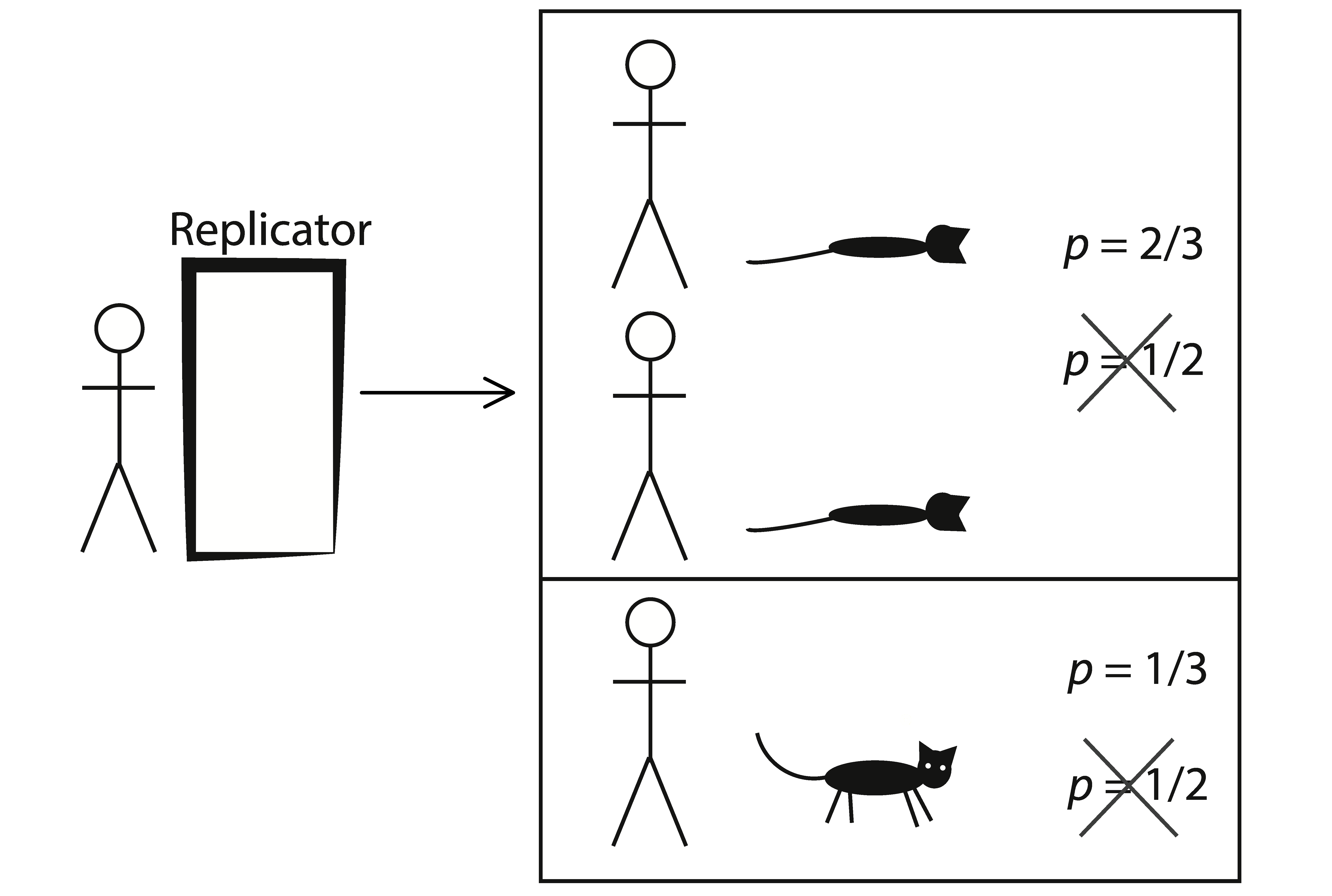
Figure 1: Replicator: 2 outcomes, 3 indistinguishables $\Longrightarrow$ 3 counts in 2 categories.

How these copies are categorized into indistinguishable outcomes does not determine the objective entities being counted. There are two such outcomes, which are subjective categories, not objective countables. This is no different than any classical count, like the proverbial marbles being chosen out of a bag. If there are 7 red and 3 blue marbles in the bag, and one marble is chosen at random, there is a $\nicefrac{{7}}{{10}}$ chance of picking a red marble. This is based on an objective count of marbles, even though we are asking for the probability of a subjective category, such as colour. Thus, based on objective counts, the probability of seeing a live cat should be placed at $\nicefrac{{1}}{{3}}$. Yet, counting subjective outcomes, we would say the probability was $\nicefrac{{1}}{{2}}$, since there are two distinct outcomes, one a living cat and one a dead cat. In this case, however, it seems clear that one should count copies, categorized into outcomes, rather than count the outcomes themselves. We want to count what really exists (copies) not our subjective categories. Counting amplitudes (which leads to the Born rule) is akin to counting physical copies in the Replicator experiment, rather than categories of copies like “dead cat” and “live cat”.

2.2 Sleeping Beauty

The Sleeping Beauty experiment is shown in Figure 2. Sleeping Beauty is a subject in a sleep lab. She enters the lab on Sunday, and is told (truthfully) about everything that is to happen to her. A coin is flipped, but she is not yet told the outcome. Whatever the result of the flip, she goes to sleep on Sunday night and wakes up on Monday morning. She is then asked what the probability is that the coin flip was heads. Only after she responds is she shown the value of the coin flip. If the value was heads, she is then sent home and the experiment is over. If the value was tails, however, she is given an amnesia drug and sent to bed again, so that she wakes up on Tuesday morning with no memory of anything that happened on Monday (she still remembers everything from Sunday night, however). Again, she is asked what the probability is that the coin flip was heads, and only after she responds is she shown the result.

The puzzle here is whether she should (if she is rational) choose $\nicefrac{{1}}{{3}}$ or $\nicefrac{{1}}{{2}}$ as the probability of heads (call it $p(\textrm{H}))$. There is, in fact, no clear consensus in the literature as to the correct answer. Given the Replicator experiment, we might expect the answer to be $\nicefrac{{1}}{{3}}$, since this seems to be an exactly analogous situation: two outcomes resulting from three subjectively indistinguishable states.

Figure 2: Sleeping Beauty: 2 outcomes, 3 indistinguishables $\Longrightarrow$ 2 counts in 2 categories.

However, the cases are not as analogous as they first appear, especially if we want to use objective classical counts. There are two conflicting solutions in the literature to the Sleeping Beauty puzzle. The “Thirder” position [3] holds that $p\left(\textrm{H}\right)=\nicefrac{{1}}{{3}}$, as there are three objectively distinct (countable), but subjectively indistinguishable situations, only one with heads, so the probability is $\nicefrac{{1}}{{3}}$ (or so say the Thirders). This sounds exactly like the argument made for the Replicator example (but we will see that it is not).

The other position (the “Halfer” viewpoint [10]) is that the probability is $\nicefrac{{1}}{{2}}$, since Sleeping Beauty clearly believed that $p\left(\textrm{H}\right)=\nicefrac{{1}}{{2}}$ on Sunday night before going to bed. Yet, when she wakes up, everything is exactly as she expected, so far as she can tell. Thus, she receives no new information, and her degree of uncertainty (and hence her probabilities) cannot possible have changed, and $p\left(\textrm{H}\right)$ must remain at $\nicefrac{{1}}{{2}}$ (or so say the Halfers).

It has been argued [11, 14] that an Everettian must be a Halfer. I agree with this position, and would further contend that if we are performing classical counts at all, we must be Halfers. I argue this in spite of the similarity between the Thirder solution and the Replicator experiment, which is really merely apparent. The key difference between the two examples is that, although in both cases there are three objectively distinct cases, in the Replicator, the actual generation of the cases occurs at the generation of each physical copy. Additional uncertainty (as to which case will ultimately hold) is introduced at the generation of each such case.

In Sleeping Beauty, there is only one actual physical event that introduces uncertainty, and that is the coin flip, which generates only two objectively distinct cases. After that, a third case is “pseudo-generated” by the application of the drug, but this does not actually generate an objectively distinct case, and thus not one that can be objectively counted. There are only two objectively distinct cases for Beauty, whereas for the Replicated observer, there really are three physical copies.

3 The Generative Principle

This idea that we count possibilities that are generated by a process was put forward by Popper [13] as a potential classical-count-based solution to the problem of quantum probability. However, he rejected generativism because he felt that it violated the principle of indifference required for classical counts, and this pushed him towards his propensity interpretation. I believe he erred because he did not consider algorithmic probability, which justifies its counts with LaPlacian indifference, yet still ends up with apparently unequal probabilities for its possibilities. I do not claim here to definitively argue for generativism, but see [14, Ch4] for my detailed arguments, where I argue that it is the best approach to the objective probabilities being sought in the Everett interpretation, or in any other classical counting method for computing probabilities.

Both the Replicator and Sleeping Beauty can be formulated generatively, even though the former is about objective probability and the latter is about subjective probability. This is based on the fact that, as with state supervenience [19], even though probabilities are subjective, we still assume there is some committment on the part of the subject to basing their probabilities on their (possibly partial) knowledge of what they take to be the objective state of affairs. We can state this principle in terms of the use of coarse-grained and fine-grained models:

The Generative Probability Principle: agents are taken to use internal “models” of their environment in making decisions. Rational agents will assign subjective probabilities (“credences”), in any coarse-grained model involving uncertainties, in exactly the same way they assign objective probabilities (“chances”) in a finer-grained model with no uncertainty. Alternative scenarios that are due to uncertainty in the model can be replaced with literal copies of the observer and their environment—one for each scenario—to turn the probabilities into objective probabilities and eliminate subjective credences, without affecting the probabilities.

So Sleeping Beauty’s credences can be calculated using classical counts, by turning her scenario into a Replicator scenario, in which the two options (heads and tails) both literally happen, by copying Sleeping Beauty and the whole sleep lab in a replicator machine. Note that we need to “copy” the entire environment, not just the observer, to avoid possible complications of interacting observers.

While this copying process turns the problem into the same kind of probability problem as the Replicator, it isn’t necessarily clear whether it answers the debate between the Halfers and the Thirders. The Thirders might insist, now that we’ve copied the Sleep Lab, that we might just as well replace the amnesia drug with a copying process, as well, which would then settle things definitively in favour of the Thirders. However, this would violate the Generative Principle, which tells us to only use copying to replace uncertainty in the model. Self-locating uncertainty is a different kind of thing altogether (at least, in the Halfer view). Agents are bound rationally to act in accord with how they think the real world works, so uncertainty in the world model can be replaced with real copying of worlds (or at least sleep labs). However, uncertainty due to amnesia is purely due to a mental mistake, and does not introduce any further uncertainty into the model. Remember that Sleeping Beauty knows about the amnesia drug. Her forgetfulness does not change what she knows about how the experiment works.

In the Halfer view, waking up with amnesia has no effect on Beauty’s world model and brings no new information in, so cannot change the probabilities. Nonetheless, the amnesia process obviously still could come into play in the calculation of probabilities. If we show Sleeping Beauty on Tuesday morning the coin, that it is tails, she still doesn’t know whether it is Monday or Tuesday, and this uncertainty is completely due to the drug. Nonetheless, when we ask her what the probability is that it is Tuesday, she uses the principle of indifference to assign equal credences, and replies that the probability is 50%. She could imagine a replicator copying process in doing so. But she can’t do a copying process before we tell her the result is tails, because then she would be mixing uncertainty in the model and self-locating uncertainty. Once you have calulcated all your measures via copying, if there is still self-locating doubt within a copied “branch”, then a simple application of indifference is permitted, even though not generative.

The above is not a thorough defence of Halferism, and neither is it intended to be, as I have argued my position elsewhere [14]. My goal here is to show the effect the generative principle has on the Replicator and Sleeping Beauty experiments, assuming that Halferism is correct, with an eye to applying the ideas to subjective quantum probability.

4 Solomonoff Probability

Solomonoff (algorithmic) probability [16, 17] is the natural result of taking generative probability to its logical conclusion, since programs are the epitome of a formal generative process. Solomonoff probability can be defined in terms of classical probability counts, where the objects counted are abstract computer programs. The algorithmic “information” or “entropy” $H\left(x\right)$, of a code or symbol sequence $x$, is the average number of bits in any program that generates $x$, given a computer programming language $\mathcal{L}$:

$$H\left(x|\mathcal{L}\right) =-\log_{2}p\left(x|\mathcal{L}\right)$$

$$p(x|\mathcal{L}) =\lim_{n\rightarrow\infty}\sum_{g\in\mathcal{G}^{n}(x|\mathcal{L})}2^{-\left|g\right|}$$

where $\mathcal{G}(x|\mathcal{L})$ is the set of all programs in language $\mathcal{L}$ that generate (or output) $x$, which is always enumerated from least to greatest size, in bits, and $\mathcal{G}^{n}(x|\mathcal{L})$ is the subset of $\mathcal{G}(x|\mathcal{L})$ containing only programs of size $n$ bits or less.

The probability $p\left(x|\mathcal{L}\right)$ of a randomly chosen program in language $\mathcal{L}$ generating $x$ can also be written simply as

$$p\left(x|\mathcal{L}\right)=2^{-H\left(x|\mathcal{L}\right)}$$ (1)

Solomonoff proved that the required infinite sequence converges, and that it converges quickly, so that shorter programs count exponentially more to the final count than longer programs [18]. Due to this fact, the algorithmic entropy and probability functions can be approximated in terms of the single optimal compression program $c\left(x|L\right)$, defined as the shortest bit-length program written in language $\mathcal{L}$ that generates $x$:

$$H\left(x|\mathcal{L}\right) \approx\left|c\left(x|\mathcal{L}\right)\right|$$

$$p(x|\mathcal{L}) \approx 2^{-\left|c\left(x|\mathcal{L}\right)\right|}$$

I have said that in Solomonoff probability, we count programs. Yet, on the face of it, this equation seems to be doing nothing of the sort. It does not talk about the number of programs that generate a result, but rather their size. However, we can turn this into straight program counting, by considering only programs of a fixed size, and then taking this measure to the limit as the program size goes to infinity, obtaining Solomonoff’s result (I give a more rigorous explanation in [14], or see a textbook on algorithmic information theory [12]).

5 The Algorithmic Generative Principle

The generative principle can be formulated much more rigorously for Solomonoff probabilities, which have a more formal basis. Note that while I talk about sets and functions below, these are all intended to be discrete computer programming analogs to the traditional mathematical notions of sets and functions. Everything here is a discrete data structure, and there are no completed infinities.

1. Assume an observer in a given pre-observation state $m$.

2. Define a (Turing-complete) computer programming language, $\mathcal{L}=\left\{p_{1},p_{2},p_{3}\cdots p_{i}\cdots\right\},$ called the “model-language”. All relevant observer background knowledge comes with $\mathcal{L}$ as built-in language functions. The i-th program in $\mathcal{L}$, called a “model-program”, is $p_{i}$ (under some enumeration of the language, from smallest to largest sized programs, in bits).

3. Define the set $\mathcal{M}=\left\{m_{k}\right\}$ of all possible observer states that are, to the observer. subjectively indistinguishable from $m$ (including $m$ itself).

4. Define set $\mathcal{I=}\left\{i_{k}\right\}$ of “situations”, which are model-programs that generate the observer in the pre-observation state $m$, and also generate at least one post-observation “continuer” state, representing a “result” $r$ of the observation from the perspective of $m$. Each situation $i_{k}$ yields a different set of results.

5. Define set $\mathcal{S=}\left\{s_{k}\right\}$ of “scenarios”. A scenario is a set of all situations that generates results for any member of $\mathcal{M}$ (any pre-observation state subjectively indistinguishable from $m$).

6. Function $\mathcal{R}\left(s\right)=\left\{r_{j}\right\}$ returns a list of results $\left\{r_{j}\right\}$ generated by the running of situation or scenario $s$. $\mathcal{R}\left(\mathcal{I}\right)$ returns a list of all results for all situations in $\mathcal{I}$. Each result must be generated by the same situation that generated the pre-observation state, but there is no requirement about where or when the result needs to appear in the program state or execution. A result is always unique, so there can never be two instances of the same result.

7. Function $\mathcal{O}\left(s\right)=\left\{o_{k}\right\}$, returns a set of all “outcomes” from a given situation or scenario $s$. $\mathcal{O}\left(\mathcal{I}\right)$ and $\mathcal{O}\left(\mathcal{S}\right)$ return all outcomes for all situations in $\mathcal{I}$ and in $\mathcal{S}$, respectively. Each outcome, $o_{k}=\left\{r_{j}^{k}\right\},$ is a set of results that are subjectively indistinguishable to the observer.

8. Define $N\left(o_{k}^{\mathcal{}}|\mathcal{L}\right)$ as the number of results in $o_{k}$ that are generated by the optimal compression $c\left(o_{k}|\mathcal{L}\right)$.

9. Define $N\left(o_{k}|\mathcal{M}|\mathcal{L}\right)$ as the number of members, or generators, of $o_{k}$ in $\mathcal{M}$.

10. Define a branch factor $B\left(o_{k}\right)=\frac{N\left(o_{k}^{\mathcal{}}|\mathcal{L}\right)}{N\left(o_{k}|\mathcal{M}|\mathcal{L}\right)}$.

11. Define the probability of result $r_{k}\in\mathcal{R}\left(i_{j}\right)$, given situation $i_{j}$:

    $$p\left(r_{k}|i_{j}|\mathcal{L}\right)=\frac{1}{\left|\mathcal{R}\left(i_{j}\right)\right|}\frac{}{}\frac{}{}^{\frac{}{}}$$

12. Define the algorithmic probability of outcome $o_{k}$, generated by scenario $s_{j}$, dividing the measure amongst the results of the optimal compression ($Z$ is a standard normalization constant):

    $$p(o_{k}|\mathcal{L})=\frac{1}{Z}\left(B\left(o_{k}\right)2^{-H\left(o_{k}|\mathcal{L}\right)}\right)$$

13. Divide the probability of an outcome $o_{k}$ amongst all its results in the optimal compression:

    $$p\left(r|o_{k}|\mathcal{L}\right)=\frac{p(o_{k}|\mathcal{L})}{N\left(o_{k}|\mathcal{L}\right)}$$

We can remove references to $\mathcal{L}$ when the choice of language is either arbitrary or clear from the context. Note that the probability of a result is classical, not algorithmic, because there is only a single program code (or situation) in play. The probability of a particular outcome needs to be shared between all of its constituent results in the optimal compression. This is because algorithmic probability alone does not cover this situation. The principle of indifference, however, demands that we simply divide our measure evenly between results.

We are now ready to apply our algorithmic version of the generative principle to the Replicator and Sleeping Beauty experiments.

6 Algorithmic Replicator

The Replicator example asks us to think in terms of objective chances, with total knowledge and no uncertainty. There is thus a single situation $s$ in the model:

$$\mathcal{I=S}=\left\{s\right\}$$

There is also only one pre-observation state:

$$\mathcal{M}=m$$

The running of this single situation generates three results:

$$\mathcal{R}\left(s\right)=\left\{\textrm{cat-dead-1},\textrm{ cat-dead-2, cat-alive}\right\}$$

This generates two outcomes based on subjective indistinguishability:

$$\mathcal{O}\left(s\right) =\left\{\textrm{cat-dead},\textrm{cat-alive}\right\}=\left\{\textrm{$\left\{\textrm{cat-dead-1},\textrm{cat-dead-2}\right\}$ },\left\{\textrm{cat-alive}\right\}\right\}$$

The probabilities for our three results are all equal since we have only one situation:

$$p\left(\textrm{cat-dead-1}|s\right)=p\left(\textrm{cat-dead-2}|s\right)=p\left(\textrm{cat-alive}|s\right)=\frac{1}{\left|\mathcal{R}\left(s\right)\right|}=\frac{1}{3}$$

Calculating the branch factors:

$$B\left(\textrm{cat-dead}\right) =\frac{N\left(\textrm{cat-dead}\right)}{N\left(\textrm{cat-dead}|\mathcal{M}\right)}=\frac{2}{1}=2$$

$$B\left(\textrm{cat-alive}\right) =\frac{N\left(\textrm{cat-alive}\right)}{N\left(\textrm{cat-alive}|\mathcal{M}\right)}=\frac{1}{1}=1$$

Since there is only situation, everything compresses to it, and the exact size of the optimal compression does not matter. Let’s say, without loss of generality, that it takes 3 bits to represent $s$:

$$p(\textrm{cat-dead}) =\frac{1}{Z}\left(B\left(\textrm{cat-dead}\right)2^{-H\left(\left\{\textrm{cat-dead-1},\textrm{cat-dead-2}\right\}\right)}\right)=\frac{1}{Z}\left(2\left(2^{-3}\right)\right)=\frac{\nicefrac{{1}}{{4}}}{\nicefrac{{1}}{{4}}+\nicefrac{{1}}{{8}}}=\frac{2}{3}$$

$$p(\textrm{cat-alive}) =\frac{1}{Z}\left(B\left(\textrm{{{cat-alive}}}\right)2^{-H\left(\left\{\textrm{cat-alive}\right\}\right)}\right)=\frac{1}{Z}\left(1\left(2^{-3}\right)\right)=\frac{\nicefrac{{1}}{{8}}}{\nicefrac{{1}}{{4}}+\nicefrac{{1}}{{8}}}=\frac{1}{3}$$

Finally, if we want to know the probability of ending up as each of the three individual copies:

$$p(\textrm{cat-dead-1})=p(\textrm{cat-dead-2})=p\left(\textrm{cat-dead-1}|\left\{\textrm{cat-dead-1},\textrm{cat-dead-2}\right\}\right)$$

$$=\frac{p(\left\{\textrm{cat-dead-1},\textrm{cat-dead-2}\right\})}{N\left(\left\{\textrm{cat-dead-1},\textrm{cat-dead-2}\right\}\right)}=\left(\frac{\nicefrac{{2}}{{3}}}{2}\right)=\frac{1}{3}$$

$$p(\textrm{cat-alive})=p\left(\textrm{cat-alive}|\left\{\textrm{cat-alive}\right\}\right)=\frac{p(\left\{\textrm{cat-alive}\right\})}{N\left(\left\{\textrm{cat-alive}\right\}\right)}=\left(\frac{\nicefrac{{1}}{{3}}}{1}\right)=\frac{1}{3}$$

7 Algorithmic Sleeping Beauty

Sleeping Beauty asks us to think in terms of subjective credences, with uncertainty and incomplete knowledge. There are two situations in this model, in one scenario, H (for heads) and T (for tails):

$$\mathcal{S=}\left\{\textrm{H},\textrm{T}\right\}$$

Although the thought experiment asks for $p\left(\textrm{H}\right)$, there are actually two such probabilities in the problem. We have $p_{\textrm{SUN}}\left(\textrm{H}\right)=\nicefrac{{1}}{{2}}$ on Sunday night. Everyone agrees on this result. The $p\left(\textrm{H}\right)$ that is in question is the one on awakening (on Monday or Tuesday morning), so it is this $p\left(\textrm{H}\right)$ we will analyze in terms of the generative model.

In “the morning” (which could actually be either Monday or Tuesday morning), there are three pre-observation states, subjectively indistinguishable one from the other:

$$\mathcal{M}=\left\{\textrm{H}_{\textrm{Mon}},\textrm{T}_{\textrm{Mon}},\textrm{T}_{\textrm{Tue}}\right\}$$

There are still two situations, since the uncertainty of the coin flip means two alternative processes may occur, and we capture them as two model-programs. The running of the two different situations yields three different results in total:

$$\mathcal{R}\left(\textrm{H}\right) =\left\{\textrm{H}_{\textrm{Mon}}\right\} \mathcal{R}\left(\textrm{T}\right) =\left\{\textrm{T}_{\textrm{Mon}},\textrm{T}_{\textrm{Tue}}\right\} \mathcal{R}\left(\mathcal{S}\right)=\left\{\textrm{H}_{\textrm{Mon}},\textrm{T}_{\textrm{Mon}},\textrm{T}_{\textrm{Tue}}\right\}$$

This generates two outcomes, based on subjective indistinguishability, but containing differing numbers of results depending on the situation or scenario:

$$\mathcal{O}\left(\textrm{H}\right)=\left\{\mathcal{H}\right\},\textrm{$\mathcal{H}$}=\left\{\textrm{H}_{\textrm{Mon}}\right\}$$

$$\mathcal{O}\left(\textrm{T}\right)=\left\{\mathcal{T}\right\},\textrm{$\mathcal{T}$}=\left\{\textrm{T}_{\textrm{Mon}},\textrm{T}_{\textrm{Tue}}\right\}$$

$$\mathcal{O}\left(\mathcal{S}\right)=\left\{\textrm{$\mathcal{H}$},\mathcal{T}\right\}=\left\{\left\{\textrm{H}_{\textrm{Mon}}\right\},\left\{\textrm{T}_{\textrm{Mon}},\textrm{T}_{\textrm{Tue}}\right\}\right\}$$

The probabilities for our three results within their given situations are:

$$p\left(\textrm{H}_{\textrm{Mon}}|\textrm{H}\right) =\frac{1}{\left|\mathcal{R}\left(\textrm{H}\right)\right|}=1$$

$$p\left(\textrm{T}_{\textrm{Mon}}|\textrm{T}\right)=p\left(\textrm{T}_{\textrm{Tue}}|\textrm{T}\right) =\frac{1}{\left|\mathcal{R}\left(\textrm{T}\right)\right|}=\frac{1}{2}$$

Since there are two situations, we need to be concerned with which one is the optimal compression. However, it is easy in this case, to see that the bit-counts should be the same, since it is only a coin flip that distinguishes them. So, as before, assume a bit-length of $3$, without loss of generality.

Calculating the branch factors:

$$B\left(\mathcal{H}\right) =\frac{N\left(\mathcal{H}\right)}{N\left(\mathcal{H}|\mathcal{M}\right)}=\frac{1}{1}=1 B\left(\mathcal{T}\right)=\frac{N\left(\mathcal{T}\right)}{N\left(\textrm{$\mathcal{T}$}|\mathcal{M}\right)}=\frac{2}{2}=1$$

So the algorithmic probabilities of the outcomes are:

$$p(\mathcal{H}) =\frac{1}{Z}\left(B\left(\mathcal{H}\right)2^{-H\left(\mathcal{H}\right)}\right)=\frac{1}{Z}\left(\left(1\right)2^{-3}\right)=\frac{\nicefrac{{1}}{{8}}}{\nicefrac{{1}}{{8}}+\nicefrac{{1}}{{8}}}=\frac{1}{2}$$

$$p(\mathcal{T}) =\frac{1}{Z}\left(B\left(\mathcal{T}\right)2^{-H\left(\mathcal{T}\right)}\right)=\frac{1}{Z}\left(\left(1\right)2^{-3}\right)=\frac{\nicefrac{{1}}{{8}}}{\nicefrac{{1}}{{8}}+\nicefrac{{1}}{{8}}}=\frac{1}{2}$$

Finally, if we want to know the probability of ending up as each of the three individual copies:

$$p(\textrm{$\textrm{H}_{\textrm{Mon}}$}|\mathcal{H}) =\frac{p(\mathcal{H})}{N\left(\mathcal{H}\right)}=\left(\frac{\nicefrac{{1}}{{2}}}{1}\right)=\frac{1}{2}$$

$$p(\textrm{$\textrm{T}_{\textrm{Mon}}$}|\mathcal{T}) =\frac{p(\mathcal{T})}{N\left(\mathcal{T}\right)}=\left(\frac{\nicefrac{{1}}{{2}}}{2}\right)=\frac{1}{4}$$

$$p(\textrm{$\textrm{T}_{\textrm{Tue}}$}|\mathcal{T}) =\frac{p(\mathcal{T})}{N\left(\mathcal{T}\right)}=\left(\frac{\nicefrac{{1}}{{2}}}{2}\right)=\frac{1}{4}$$

The algorithmic generative principle agrees with the Halfer result, since $p\left(\mathcal{H}\right)=\nicefrac{{1}}{{2}}.$

So generativism yields Halferism and, for the Replicator, copy-counting. What makes this tricky in a quantum context is that these results seem to involve both branch or outcome counting (violating the Born rule) as well as objective entity counting (leading to the Born rule). The Replicator result looks like outcome-counting, but really counts entities. Sleeping Beauty, under Halferism, counts entities for $p\left(\textrm{H}\right)$, but to distinguish between $\textrm{T}_{\textrm{Mon}}$ and $\textrm{T}_{\textrm{Tue}}$, counts outcomes within a single entity. Thus, we have combined two counting measures: (1) entity-counting, which uses Solomonoff, and (2) branch-counting within an entity. Quantum probability realistically only needs measure #1 (corresponding to amplitude-counting and the Born rule), and not the latter (corresponding to branch-counting, violating the Born rule, and only needed in quantum mechanics if people really are getting copied within a single branch).

8 Objectivity

One potential problem with the algorithmic measure is the question of its objectivity. Even when using it to calculate subjective credences, we are citing its objectivity to justify its use by claiming it is the choice a rational agent will make. Yet, the choice of language $\mathcal{L}$ does not seem to have an objective basis. I have thus far assumed that we have adopted a particular computational language in which to encode our programs, yielding a particular bit-count for any program. However, choice of a different language will yield different bit counts and hence a different probability measure. Nonetheless, Solomonoff’s invariance theorem [18] proves that the measure is invariant between languages, up to an additive constant given by the size of the translation manual between the languages. Thus, for simple languages, such as Turing machines, cellular automata or (especially) $\lambda$-calculus, it does seem that the measure should be very close to an objective measure.

In the case of the replicator copies, probability is objective (“ontic”) since there really are three physically distinct cases, and thus three physically distinct sequences of events happening simultaneously. In the case of the coin flip, probability is subjective (“epistemic”) since there is only one actual, deterministic sequence of events, which Beauty could predict with complete certainty if she knew everything about it. However, given the state of her knowledge, she builds a generative model—a mental algorithm of the situation—that models the coin flip as a random event that generates two objectively distinct scenarios. The so-called “third” event on Tuesday morning she knows is not a real third alternative, even though when she is actually in the situation she cannot tell the difference. Her model of reality provides the countable, not her number of indistinguishable mental states. The fact that we build generative (and I would argue, ideally computational) models of reality is what allows us to make rational choices based on our uncertainty, by treating our models as if they were real, for all intents and purposes, even though we know they are not.

9 Algorithmic Objective Quantum Probability

Algorithmic probability has the potential to facilitate a derivation of quantum probability and the Born rule for both the objectivist approach (as in [14]) and a subjectivist approach (as in [19]), as well approaches in between these extremes. This is because the use of algorithms to express subjective priors implies a generative model on the part of the observer, which means that they are essentially already making an assumption something like the decision-theoretic state supervenience assumption of [19] or our algorithmic generative principle.

Algorithmic probability is based on the idea of data compression, and I have shown elsewhere in detail how this can be used to formulate quantum probability [14, 15] under objectivist Everettian assumption, so I will only review the idea briefly here. The main equation for quantum dynamics is the Schrödinger equation, and the solved, discrete (digitized) form of this is the discrete Fourier transform (DFT), widely used in data compression, and particularly ubiquitous in the (lossy) compression of perceptual data, such as video and audio.

These features of the DFT are used as a basis for my objectivist Born rule proof in [14]. If we assume that the optimal compression of an observer’s state is essentially a DFT, then this puts us directly into the inner product vector space of quantum mechanics. And the fact that we use a count-based objectivist notion of probability to do this justifies the Born rule for much the same reason that state supervenience does, but by appealing to Gleason’s theorem [5, 14].

A key feature of DFT-based compression that gives it potential explanatory power in this scheme is the fact that it is “lossy”. Assume I use it to compress a digital picture of my grandmother. I am essentially searching for the “shortest program” that generates an image sufficiently recognizable as my grandmother. Since I value shortness, and shorter compression results in lower quality decompressions, the decompressed image should (let us say) be as low quality as possible, while still being recognizable as my grandmother. Shorter programs use fewer DFT frequencies and have more “artifacts” in the resulting image (pixelations, fuzziness, etc.). I argue in [15, 14] that our goal in digital quantum probability is to compress the observer’s mental state as much as possible while still retaining enough fidelity that decompression will regenerate the same conscious state. Beyond that, we are fine with artifacting if it permits the program size to be minimized. Thus, there is a distinct possibility that the rest of the universe—the wide environment around our conscious mental states—is nothing but digital artifacting of this decompression.

10 Algorithmic Subjective Quantum Probability

This objectivist use of algorithmic probability in quantum mechanics is fundamentally Everettian, since the only way that counting programs can be objective is if $\mathcal{L}$, representing our background knowledge, is an extremely simple language, such as $\lambda$-calculus (which choice might presumably be acceptable prima facie on the basis of Occam’s razor). The only way to rid ourselves of the excessive baggage of world knowledge is to make our world knowledge so simple and general that it cannot possibly be taken as anything but a model of rationality. Under this view, however, our counts must be of real existing entities, and so the abstract programs we are counting become the ontic (objectively existing) entities of reality, which leads to Everettianism, or at least to some other version of idealism.

The downside of this, for some, is the extravagant cosmology and metaphysics implied. And while I do not wish to get into a discussion of the pros and cons here, I would like to suggest that it may be possible to retain many of the advantages of this algorithmic framework even whilst switching to a far more subjectivist interpretation of probability. It is common in Solomonoff probability to permit even complex languages for $\mathcal{L}$ , since these can be interpreted as a way of setting priors in a subjectivist Bayesian scheme. Moreover, because our models are still world models, and priors are set in a rationally justified way, this may be enough objectivism to still provide something akin to state supervenience and permit a derivation of the Born rule. Moreover, as we “tune” our DFT model by choosing more objective or more subjective programming languages, we get something more like an Everettian or many-worlds interpretation on the one end, and something more like quantum Bayesianism [2] on the other, permitting a wide spectrum of interpretations along the objectivist-subjectivist spectrum.

Indeed, the whole spectrum between objective and subjective measures corresponds precisely to a spectrum between simple and complex programming languages, which in a quantum context we may speculate yields a DFT compression algorithm, in turn yielding a discrete version of Schrödinger’s dynamical equation. This holds the promise, perhaps, of a single conception of probability that may usefully be applied to many different quantum interpretations, just as we applied it to both the Everett-like Replicator and the Bayesian-style Sleeping Beauty. The utility of such a common ground in quantum foundations discourse could be high, given the extent to which different positions and arguments in the field tend to be driven by radically different conceptions of probability.

References

- [1]
- [2] Carlton M Caves, Christopher M Fuchs & Ruediger Schack (2002): Quantum probabilities as Bayesian probabilities. Physical Review A 65, 10.1103/PhysRevA.65.022305.
- [3] Adam Elga (2000): Self-locating belief and the Sleeping Beauty problem. Analysis 60(2), pp. 143–147, 10.1093/analys/60.2.143.
- [4] Hugh Everett III (1957): ’Relative state’ formulation of quantum mechanics. Reviews of Modern Physics 29, pp. 454–462, 10.1103/RevModPhys.29.454.
- [5] A Gleason (1957): Measures on the closed subspaces of a Hilbert space. Journal of Mathematics and Mechanics 6(6), pp. 885–893, 10.1512/iumj.1957.6.56050.
- [6] S Gutmann (1995): Using classical probability to guarantee properties of infinite quantum sequences. Physical Review A 52(5), pp. 3560–3562, 10.1103/PhysRevA.52.3560. Available at http://arxiv.org/abs/quant-ph/9506016.
- [7] J B Hartle (1968): Quantum Mechanics of Individual Systems. American Journal of Physics 36(8), pp. 704–712, 10.1119/1.1975096.
- [8] Pierre Simon Marquis de Laplace (1902): A Philosophical Essay on Probabilities (1814). John Wiley & Sons, New York.
- [9] Gottfried Wilhelm von Leibniz (2006): Estimating the Uncertain (1678). In Marcelo Dascal, editor: The Art of Controversies, Springer, pp. 105–118, 10.1007/1-4020-5228-6.
- [10] David Lewis (2001): Sleeping Beauty. Analysis 61(3), pp. 171–187, 10.1093/analys/61.3.171.
- [11] Peter J Lewis (2007): Quantum Sleeping Beauty. Analysis 67(293), pp. 59–65, 10.1111/j.1467-8284.2006.00597.x.
- [12] Ming Li & P M B Vitányi (2008): An introduction to Kolmogorov complexity and its applications. Springer, New York, 10.1007/978-0-387-49820-1.
- [13] Karl Popper (1959): The propensity interpretation of probability. The British Journal for the Philosophy of Science 10(37), pp. 25–42, 10.1093/bjps/X.37.25.
- [14] Allan F Randall (2014): An Algorithmic Interpretation of Quantum Probability. Ph.D. thesis, York University, Toronto, Available at http://hdl.handle.net/10315/27640.
- [15] Allan F Randall (2016): Quantum Probability as an Application of Data Compression Principles. Electronic Proceedings in Theoretical Computer Science 214(12), pp. 29–40, 10.4204/EPTCS.214.6.
- [16] Ray Solomonoff (1960): A Preliminary Report on a General Theory of Inductive Inference. Zator Company and United States Air Force Office of Scientific Research, ZTB-138, Cambridge. Available at http://world.std.com/~rjs/publications/z138.pdf.
- [17] Ray Solomonoff (1964): A formal theory of inductive inference: parts 1 and 2. Information and Control 7(1-2), pp. 1–22 & 224–254, 10.1016/S0019-9958(64)90131-7.
- [18] Ray Solomonoff (1978): Complexity-based induction systems: comparisons and convergence theorems. IEEE Transactions on Information Theory 24(4), pp. 422–432, 10.1109/TIT.1978.1055913. Available at http://world.std.com/~rjs/publications/solo1.pdf.
- [19] David Wallace (2010): How to prove the Born rule. In S. Saunders, J. Barrett, A. Kent & D. Wallace, editors: Many Worlds? Everett, Quantum Theory, and Reality, Oxford University Press, Oxford, pp. 227–263, 10.1093/acprof:oso/9780199560561.003.0010. Available at http://arxiv.org/abs/0906.2718.