Fast and Accurate Sensitivity Estimation for Continuous-Gravitational-Wave Searches

Abstract

This paper presents an efficient numerical sensitivity-estimation method and implementation for continuous-gravitational-wave searches, extending and generalizing an earlier analytic approach by Wette Wette (2012). This estimation framework applies to a broad class of $\mathcal{F}$-statistic-based search methods, namely (i) semi-coherent StackSlide $\mathcal{F}$-statistic (single-stage and hierarchical multi-stage), (ii) Hough number count on $\mathcal{F}$-statistics, as well as (iii) Bayesian upper limits on (coherent or semi-coherent) $\mathcal{F}$-statistic search results. We test this estimate against results from Monte-Carlo simulations assuming Gaussian noise. We find the agreement to be within a few $\%$ at high (i.e. low false-alarm) detection thresholds, with increasing deviations at decreasing (i.e. higher false-alarm) detection thresholds, which can be understood in terms of the approximations used in the estimate. We also provide an extensive summary of sensitivity depths achieved in past continuous-gravitational-wave searches (derived from the published upper limits). For the $\mathcal{F}$-statistic-based searches where our sensitivity estimate is applicable, we find an average relative deviation to the published upper limits of less than $10\%$, which in most cases includes systematic uncertainty about the noise-floor estimate used in the published upper limits.

I Introduction

The recent detections of gravitational waves from merging binary-black-hole and double neutron-star systems Abbott et al. (2016a, b, 2017a) have opened a whole new observational window for astronomy, allowing for new tests of general relativity Abbott et al. (2016c), new constraints on neutron star physics Abbott et al. (2018a) and new measurements of the Hubble constant Abbott et al. (2017b), to mention just a few highlights.

Continuous gravitational waves (CWs) from spinning non-axisymmetric neutron stars represent a different class of potentially-observable signals Prix (2009); Lasky (2015), which have yet to be detected Riles (2017). These signals are expected to be long-lasting (at least several days to years) and quasi monochromatic, with slowly changing (intrinsic) frequency. The signal amplitude depends on the rich (and largely not yet well-understood) internal physics of neutron stars Johnson-McDaniel and Owen (2013), as well as their population characteristics Camenzind (2007); Knispel and Allen (2008). A detection (and even non-detection) of CWs could therefore help us better understand these fascinating astrophysical objects, and may allow for new tests of general relativity Isi et al. (2017); Abbott et al. (2018b).

Overview of search categories

We can categorize CW searches in two different ways: either based on the search method, or on the type of explored parameter space.

The search methods fall into two broad categories: coherent and semi-coherent (sometimes also referred to as incoherent). Roughly speaking, a coherent search is based on signal templates with coherent phase evolution over the whole observation time, while semi-coherent searches typically break the data into shorter coherent segments and combine the resulting statistics from these segments incoherently (i.e. without requiring a consistent phase evolution across segments). However, there are many different approaches and variations, which are beyond the scope of this paper, see e.g. Riles (2017) for a more detailed overview. Here we will exclusively focus on coherent and semi-coherent methods based on the $\mathcal{F}$-statistic, which will be introduced in Sec. II.

Coherent search methods are the more sensitive in principle, but in practice they usually suffer from severe computing-cost limitations: for finite search parameter spaces the required number of signal templates typically grows as a steep power-law of the observation time, making such searches infeasible except when the search region is sufficiently small. For larger signal parameter spaces the observation time needs to be kept short enough for the search to be computationally feasible, which limits the attainable coherent sensitivity. This is where semi-coherent searches tend to yield substantially better sensitivity at fixed computing cost (e.g. see Brady and Creighton (2000); Prix and Shaltev (2012)).

Based on the explored parameter space, we distinguish the following search categories (referencing a recent example for each case):

1. Targeted searches for known pulsars Manchester et al. (2005) assume a perfect fixed relationship between the observed neutron-star spin frequency and the CW emission frequency. Therefore one only needs to search a single point in parameter space for each pulsar, allowing for optimal fully-coherent searches Abbott et al. (2017c).

2. Narrow-band searches for known pulsars assume a small uncertainty in the relationship between CW frequency and the measured pulsar spin rates. This finite search parameter space requires a template bank with (typically) many millions of templates, still allowing for optimal fully-coherent search methods to be used Abbott et al. (2017d).

3. Directed (isolated) searches aim at isolated neutron stars with known sky-position and unknown spin frequency. The search parameter space covers the unknown frequency and spindowns of the neutron star signal within an astrophysically-motivated range Aasi et al. (2015a); Zhu et al. (2016).

4. (Directed) binary searches aim at binary systems with known sky-position and parameter-space uncertainties in the frequency and binary-orbital parameters. Typically these sources would be in low-mass X-ray binaries, with the most prominent example being Scorpius X-1 (Sco X-1)) Abbott et al. (2017e, f).

5. All-sky (isolated) searches search the whole sky over a large frequency (and spindown) band for unknown isolated neutron stars Abbott et al. (2017a, b).

6. All-sky binary searches are the most extreme case, covering the whole sky for unknown neutron stars in binary systems Goetz and Riles (2011); Aasi et al. (2014a).

Sensitivity estimation

In this work we use the term sensitivity to refer to the upper limit on signal ampltitude $h_{0}$ (or equivalently sensitivity depth $0pt\equiv\sqrt{S_{\mathrm{n}}}/h_{0}$, see Sec. II.5). This can be either the frequentist upper limit for a given detection probability at a fixed false-alarm level (p-value), or the Bayesian upper limit at a given credible level for the given data.

Sensitivity therefore only captures one aspect of a search, namely how “deep” into the noise-floor it can detect signals, without accounting for how “wide” a region in parameter space is covered, how much prior weight this region contains, or how robust the search is to deviations from the signal model. Comparing sensitivity depth therefore only makes sense for searches over very similar parameter spaces. A more complete measure characterizing searches would be their respective detection probability, which folds in sensitivity depth, breadth in parameter space, as well as the prior weight contained in that space Ming et al. (2016, 2018).

However, it is often useful to be able to reliably and cheaply estimate the sensitivity of a search setup without needing expensive Monte-Carlo simulations:

• In order to determine optimal search parameters for a semi-coherent search (i.e. the number and semi-coherent segments and template-bank mismatch parameters), it is important to be able to quickly asses the projected sensitivity for any given search-parameter combination (e.g. see Prix and Shaltev (2012); Leaci and Prix (2015); Ming et al. (2016, 2018)).

• For setting upper limits for a given search, one typically has to repeatedly add software-generated CW signals to the data and perform a search, in order to measure how often these signals are recovered above a given threshold. By iterating this procedure one tries to find the weakest signal amplitude that can be recovered at the desired detection probability (or “confidence”). This can be very computationally expensive, and a quick and reasonably-reliable estimate for the expected upper-limit amplitude can therefore substantially cut down on the cost of this iterative process, which can also improve the accuracy of the upper limit.

• The estimate can also serve as a sanity check for determining upper limits.

A number of theoretical sensitivity estimates have been developed over the past decades. One of the first estimates was obtained for a coherent $\mathcal{F}$-statistic search Abbott et al. (2004), yielding

$$h_{0}=11.4\sqrt{\frac{S_{\mathrm{n}}}{T_{\mathrm{data}}}}\,,$$ (1)

for a $90\%$ confidence upper limit at $1\%$ false-alarm (per template). $S_{\mathrm{n}}$ denotes the (single-sided) noise power spectral density, and $T_{\mathrm{data}}$ is the total amount of data. This was later generalized to the semi-coherent Hough Krishnan et al. (2004) and StackSlide method Mendell and Landry (2005); Abbott et al. (2008a), yielding an expression of the form

$$h_{0}=\kappa\,N_{\mathrm{seg}}^{1/4}\,\sqrt{\frac{S_{\mathrm{n}}}{T_{\mathrm{data}}}}\,,\quad\text{with}\quad\kappa\sim 7-9\,,$$ (2)

for the same confidence and false-alarm level as Eq. (1), and where $N_{\mathrm{seg}}$ denotes the number of semi-coherent segments.

These latter results suggested the inaccurate idea that the sensitivity of semi-coherent searches follows an exact $N_{\mathrm{seg}}^{1/4}$ scaling. However, this was later shown Prix and Shaltev (2012); Wette (2012) to not be generally a good approximation except asymptotically in the limit of a large number of segments ($N_{\mathrm{seg}}\gtrsim 100-1000)$.

Furthermore, these past sensitivity estimates relied on the assumption of a “constant signal-to-noise ratio (SNR)” population of signals. While this approximation substantially simplifies the problem, it introduces a noticeable bias into the estimate, as discussed in more detail in Wette (2012). For example, the constant-SNR bias combined with the incorrect $N_{\mathrm{seg}}^{1/4}$ scaling in Eq. 2 would result in an overestimate by a factor of two of the sensitivity of the first Einstein@Home search on LIGO S5 data Aasi et al. (2013a).

These limitations of previous sensitivity estimates were eventually overcome by the analytic sensitivity-estimation method developed by Wette (2012) for semi-coherent StackSlide $\mathcal{F}$-statistic searches. In this work we simplify and extend this framework by employing a simpler direct numerical implementation. This further improves the estimation accuracy by requiring fewer approximations. It also allows us to generalize the framework to multi-stage hierarchical StackSlide-$\mathcal{F}$ searches, Hough-$\mathcal{F}$ searches (such as Aasi et al. (2013a)), as well as to Bayesian upper limits based on $\mathcal{F}$-statistic searches.

Plan of this paper

Sec. II provides a description of the CW signal model and introduces different $\mathcal{F}$-statistic-based search methods. In Sec. III we present the sensitivity-estimation framework and its implementation, for both frequentist and Bayesian upper limits. Section IV discusses how (frequentist) upper limits are typically measured using Monte-Carlo injection-recovery simulations. Section V provides comparisons of our sensitivity estimates to simulated upper limits in Gaussian noise, while in Sec. VI we provide a comprehensive summary of published sensitivities of past CW searches (translated into sensitivity depth), and a comparison to our sensitivity estimates where applicable. We summarize and discuss the results in Sec. VII. Further details on the referenced searches and upper limits are given in appendix A. More technical details on the signal model can be found in appendix B. Finally, appendix C contains a discussion of the distribution of the maximum $\mathcal{F}$-statistic over correlated templates.

II $\mathcal{F}$-statistic-based search methods

This section provides an overview of the $\mathcal{F}$-statistic-based search methods for which sensitivity estimates are derived in Sec. III. Further technical details about the signal model and the $\mathcal{F}$-statistic are given in appendix B. For a broader review of the CW signal model, assumptions and search methods, see for example Prix (2009); Lasky (2015); Riles (2017)

II.1 Signal model

For the purpose of sensitivity estimation we assume the data timeseries $x^{X}(t)$ from each detector $X$ to be described by Gaussian noise, i.e. $n^{X}(t)\sim\mathrm{Gauss}(0,S_{\mathrm{n}}^{X})$ with zero mean and (single-sided) power-spectral density (PSD) $S_{\mathrm{n}}^{X}$. A gravitational-wave signal creates an additional strain $h^{X}(t)$ in the detector, resulting in a timeseries

$$x^{X}(t)=n^{X}(t)+h^{X}(t)\,.$$ (3)

For continuous gravitational waves the two polarization components can be written as

$$\begin{split}h_{+}(\tau)=A_{+}\,\cos\left(\phi(\tau)+\phi_{0}\right)\,,\\ h_{\times}(\tau)=A_{\times}\,\sin\left(\phi(\tau)+\phi_{0}\right)\,,\end{split}$$ (4)

where $\phi(\tau)$ describes the phase evolution of the signal in the source frame. For the typical quasi-periodic signals expected from rotating neutron stars, this can be expressed as a Taylor series expansion around a chosen reference time (here $\tau_{\mathrm{ref}}=0$ for simplicity) as

$$\phi(\tau)=2\pi(f\,\tau+\frac{1}{2}\,\dot{f}\,\tau^{2}+\ldots)\,,$$ (5)

in terms of derivatives of the slowly-varying intrinsic CW frequency $f(\tau)$. For a triaxial neutron star spinning about a principal axis, the two polarization amplitudes are given by

$$A_{+}=\frac{1}{2}h_{0}\,(1+\cos^{2}\iota)\,,\quad A_{\times}=h_{0}\,\cos\iota\,,$$ (6)

in terms of the angle $\iota$ between the line of sight and the neutron star rotation axis and the overall signal amplitude $h_{0}$. This definition uses the common gauge condition of $A_{+}\geq|A_{\times}|$. After translating the source-frame signal into the detector frame (see appendix B for details), the strain signal $h^{X}(t)$ at each detector $X$ can be expressed in the factored form

$$h^{X}(t;\mathcal{A},\lambda)=\sum_{\mu=1}^{4}\mathcal{A}^{\mu}\,h^{X}_{\mu}(t;\lambda)\,,$$ (7)

which was first shown in Jaranowski et al. (1998), and where the four amplitudes $\mathcal{A}^{\mu}$ depend on the amplitude parameters $\{h_{0},\cos\iota,\psi,\phi_{0}\}$ as given in Eq. 65). The four basis functions $h_{\mu}^{X}(t;\lambda)$, which are given explicitly in Eq. (66), depend on the phase-evolution parameters $\lambda=\{\hat{n},f,\dot{f},\ldots\}$, namely sky position $\hat{n}$, frequency $f$ and its derivatives $\left.f^{(k)}=d^{k}f/d\tau^{k}\right|_{\tau_{\mathrm{ref}}}$, and binary-orbital parameters in the case of a neutron star in a binary.

II.2 Coherent $\mathcal{F}$-statistic

For pure Gaussian-noise timeseries $\{n^{X}(t)\}$ in all detectors $X$, the likelihood can be written as (e.g. seeFinn (1992); Cutler and Schutz (2005); Prix (2007)):

$$P(x=n\mid S_{\mathrm{n}})=\kappa\,e^{-\frac{1}{2}\,\left(n,n\right)}\,,$$ (8)

in terms of the multi-detector scalar product

$$\left(x,y\right)\equiv 4\operatorname{Re}\sum_{X}\int_{0}^{\infty}\frac{\tilde{x}^{X}(f)\,\tilde{y}^{X*}(f)}{S_{\mathrm{n}}^{X}(f)}\mathrm{\,d}f\,,$$ (9)

where $\tilde{x}(f)$ denotes the Fourier transform of $x(t)$, and $x^{*}$ denotes complex conjugation of $x$. Using the additivity of noise and signals (cf. Eq. (3)), we can express the likelihood for data $x$, assuming Gaussian noise plus a signal $h(\mathcal{A},\lambda)$ as

$$P(x\mid S_{\mathrm{n}},\mathcal{A},\lambda) =P(x-h(\mathcal{A},\lambda)\mid S_{\mathrm{n}})$$

$$=\kappa\,e^{-\frac{1}{2}\left((x-h),(x-h)\right)}\,.$$ (10)

From this we obtain the log-likelihood ratio between the signal and noise hypotheses as

$$\ln\Lambda(x;\mathcal{A},\lambda) \equiv\ln\frac{P(x\mid S_{\mathrm{n}},\mathcal{A},\lambda)}{P(x\mid S_{\mathrm{n}})}$$

$$=\left(x,h\right)-\frac{1}{2}\left(h,h\right)\,.$$ (11)

Analytically maximizing the log-likelihood ratio over $\mathcal{A}$ (c.f. appendix B) yields the $\mathcal{F}$-statistic Jaranowski et al. (1998):

$$\mathcal{F}(x;\lambda)\equiv\max_{\mathcal{A}}\ln\Lambda(x;\mathcal{A},\lambda)$$ (12)

The statistic $2\mathcal{F}$ follows a $\chi^{2}$-distribution with four degrees of freedom and non-centrality $\rho^{2}$,

$$P(2\mathcal{F}\mid\rho^{2})=\chi^{2}_{4}(2\mathcal{F};\rho^{2})\,,$$ (13)

with expectation and variance

$$E[2\mathcal{F}]=4+\rho^{2}\,,\quad\mathrm{var}[2\mathcal{F}]=8+4\rho^{2}\,,$$ (14)

where $\rho$ corresponds to the signal-to-noise ratio (SNR) of coherent matched filtering.

In the perfect-match case, where the template phase-evolution parameters $\lambda$ coincide with the parameters $\lambda_{\mathrm{s}}$ of a signal in the data $x$, the SNR can be explicitly expressed as

$$\rho_{0}^{2}\equiv\left(h,h\right)=\frac{4}{25}\,\frac{h_{0}^{2}}{S_{\mathrm{n}}}\,T_{\mathrm{data}}\,R^{2}(\theta)\,,$$ (15)

where $T_{\mathrm{data}}$ is the total amount (measured as time) of data over all detectors, and $S_{\mathrm{n}}$ denotes the multi-detector noise floor, defined as the harmonic mean over the per-detector PSDs $S_{\mathrm{n}}^{X}$, namely

$$\frac{1}{S_{\mathrm{n}}}\equiv\frac{1}{N}\,\sum_{X}\frac{1}{S_{\mathrm{n}}^{X}}\,.$$ (16)

Note that in practice the $\mathcal{F}$-statistic-based search implementations do not assume stationary noise over the whole observation time, but only over short durations of order $T_{\mathrm{SFT}}\sim$30\text{\,}\mathrm{m}\mathrm{i}\mathrm{n}\mathrm{s}$$, corresponding to the length of the Short Fourier Transforms (SFTs) that are typically used as input data. The present formalism can straightforwardly be extended to this case Prix (2015), where the relevant overall multi-detector noise-PSD definition $S_{\mathrm{n}}$ generalizes as the harmonic mean over all SFTs, namely

$$\frac{1}{S_{\mathrm{n}}}\equiv\frac{1}{N_{\mathrm{SFT}}}\sum_{\alpha}\frac{1}{S_{\mathrm{n}}^{\alpha}}\,,$$ (17)

where $\alpha$ is an index enumerating all SFTs (over all detectors), and $S_{\mathrm{n}}^{\alpha}$ is the corresponding noise PSD estimated for SFT $\alpha$.

The response function $R(\theta)$ (following the definition in Wette (2012)) depends on the subset of signal parameters

$$\theta\equiv\{\hat{n},\cos\iota,\psi\}\,,$$ (18)

and can be explicitly expressed Prix (2010) as

$$R^{2}(\theta)=\frac{25}{4}\left[\alpha_{1}\,A(\hat{n})+\alpha_{2}\,B(\hat{n})+2\alpha_{3}\,C(\hat{n})\right]\,,$$ (19)

with the sky-dependent antenna-pattern coefficients $\{A,B,C\}$ of Eq. (70), and

$$\alpha_{1} \equiv\frac{1}{4}\,(1+\cos^{2}\iota)^{2}\,\cos^{2}2\psi+\cos^{2}\iota\,\sin^{2}2\psi\,,$$ (20)

$$\alpha_{2} \equiv\frac{1}{4}\,(1+\cos^{2}\iota)^{2}\,\sin^{2}2\psi+\cos^{2}\iota\,\cos^{2}2\psi\,,$$ (21)

$$\alpha_{3} \equiv\frac{1}{4}\,(1-\cos^{2}\iota)^{2}\,\sin 2\psi\cos 2\psi\,.$$ (22)

One can show that $R^{2}$ averaged over $\psi\in[-\pi/4,\pi/4]$ and $\cos\iota\in[-1,1]$ yields

$$\left\langle R^{2}\right\rangle_{\cos\iota,\psi}=\frac{5}{2}\left(A(\hat{n})+B(\hat{n})\right)\,,$$ (23)

and further averaging $\hat{n}$ isotropically over the sky yields

$$\left\langle R^{2}\right\rangle_{\theta}=1\,.$$ (24)

Using this with Eq. (15) we can therefore recover the sky- and polarization-averaged squared-SNR expression (e.g. see Jaranowski et al. (1998)):

$$\left\langle\rho_{0}^{2}\right\rangle_{\theta}=\frac{4}{25}\frac{h_{0}^{2}}{S_{\mathrm{n}}}\,T_{\mathrm{data}}\,.$$ (25)

II.3 Semi-coherent $\mathcal{F}$-statistic methods

Semi-coherent methods Brady and Creighton (2000) typically divide the data into $N_{\mathrm{seg}}$ shorter segments of duration $T_{\mathrm{seg}}<T_{\mathrm{obs}}$. The segments are analyzed coherently, and the per-segment detection statistics are combined incoherently. Generally this yields lower sensitivity for the same amount of data analyzed than a fully-coherent search. However, the computational cost for a fully-coherent search over the same amount of data is often impossibly large, while the semi-coherent cost can be tuned to be affordable and typically ends up being more sensitive at fixed computing cost Brady and Creighton (2000); Cutler et al. (2005); Prix and Shaltev (2012).

There are a number of different semi-coherent methods currently in use, such as PowerFlux, FrequencyHough, SkyHough, TwoSpect, CrossCorr, Viterbi, Sideband, loosely-coherent statistics and others (e.g. see Riles (2017) and references therein). Many of these methods work on short segments, typically of length $T_{\mathrm{seg}}\sim$30\text{\,}\mathrm{m}\mathrm{i}\mathrm{n}$$, and use Fourier power in the frequency bins of these Short Fourier Transforms (SFTs) as the coherent base statistic.

In this work we focus exclusively on sensitivity estimation of $\mathcal{F}$-statistic-based methods, namely StackSlide-$\mathcal{F}$ (e.g. see Prix and Shaltev (2012)) and Hough-$\mathcal{F}$ introduced in Krishnan et al. (2004). Here the length of segments is only constrained by the available computing cost, and segments will typically span many hours to days, which yields better sensitivity, but also requires higher computational cost. Therefore, many of the computationally expensive semi-coherent $\mathcal{F}$-statistic searches are run on the distributed Einstein@Home computing platform Ein .

Note that these methods are not to be confused with the (albeit closely related) “classical” StackSlide and Hough methods, which use SFTs as coherent segments, as described for example in Abbott et al. (2008a).

II.3.1 StackSlide-$\mathcal{F}$: summing $\mathcal{F}$-statistics

The StackSlide-$\mathcal{F}$ method uses the sum of the coherent per-segment $\tilde{\mathcal{F}}$-statistic values in a given parameter-space point $\lambda$ as the detection statistic, namely

$$2\hat{\mathcal{F}}\equiv\sum_{\ell=1}^{N_{\mathrm{seg}}}2\tilde{\mathcal{F}}_{\ell}\,,$$ (26)

where $\tilde{\mathcal{F}}_{\ell}$ is the coherent $\mathcal{F}$-statistic of Eq. (12) in segment $\ell$. This statistic follows a $\chi^{2}$-distribution with $4N_{\mathrm{seg}}$ degrees of freedom and non-centrality $\rho^{2}$, i.e.

$$P(2\hat{\mathcal{F}}\mid\rho^{2})=\chi^{2}_{4N_{\mathrm{seg}}}(2\hat{\mathcal{F}};\rho^{2})\,,$$ (27)

where the non-centrality $\rho^{2}$ is identical to the expression for the coherent squared SNR of Eq. (15), with $T_{\mathrm{data}}$ referring to the whole data set used, and $S_{\mathrm{n}}$ is the corresponding noise floor. However, the non-centrality in the semi-coherent case cannot be considered a “signal to noise ratio”, due to the larger $N_{\mathrm{seg}}$-dependent degrees of freedom of the $\chi^{2}$ distribution compared to Eq. (13), which increases the false-alarm level at fixed threshold and reduces the “effective” semi-coherent $\hat{\text{SNR}}$ to $\hat{\text{SNR}}^{2}=\rho^{2}/\sqrt{N_{\mathrm{seg}}}$ (e.g. see [Eq.(14)] in Wette (2015)).

The expectation and variance for $2\hat{\mathcal{F}}$ are

$$E[2\mathcal{F}]=4N_{\mathrm{seg}}+\rho^{2}\,,\quad\mathrm{var}[2\mathcal{F}]=8N_{\mathrm{seg}}+4\rho^{2}\,.$$ (28)

We note that in practice StackSlide-$\mathcal{F}$ searches often quote the average $\overline{\mathcal{F}}$ over segments instead of the sum $\hat{\mathcal{F}}$, i.e.

$$\overline{\mathcal{F}}\equiv\frac{1}{N_{\mathrm{seg}}}\hat{\mathcal{F}}\,.$$ (29)

II.3.2 Hough-$\mathcal{F}$: summing threshold crossings

The Hough-$\mathcal{F}$ method Krishnan et al. (2004) sets a threshold $\tilde{\mathcal{F}}_{\mathrm{th}}$ on the per-segment coherent $\tilde{\mathcal{F}}$-statistics and uses the number of threshold-crossings over segments as the detection statistic, the so-called Hough number count $n_{\mathrm{c}}$, i.e.

$$n_{\mathrm{c}}\equiv\sum_{\ell=1}^{N_{\mathrm{seg}}}\Theta(\tilde{\mathcal{F}}_{\ell}-\tilde{\mathcal{F}}_{\mathrm{th}})\,,$$ (30)

where $\Theta(x)$ is the Heaviside step function.

II.4 Mismatch and template banks

In wide-parameter-space searches the unknown signal parameters $\lambda\in\mathbb{P}$ are assumed to fall somewhere within a given search space $\mathbb{P}$. In this case one needs to compute a statistic (such as those defined in the previous sections) over a whole “bank” of templates $\mathbb{T}\equiv\{\lambda_{i}\}_{i=1}^{\mathcal{N}}$. This template bank has to be chosen in such a way that any putative signal $\lambda_{\mathrm{s}}\in\mathbb{P}$ would suffer only an acceptable level of loss of SNR. This is typically quantified in terms of the so-called mismatch $\mu$, defined as the relative loss of $\rho^{2}(\lambda_{\mathrm{s}};\lambda)$ in a template $\lambda$ with respect to the perfect-match $\rho^{2}(\lambda_{\mathrm{s}};\lambda_{\mathrm{s}})=\rho_{0}^{2}$ (of Eq. (15)), namely

$$\mu(\lambda_{\mathrm{s}};\lambda)\equiv\frac{\rho^{2}(\lambda_{\mathrm{s}};\lambda_{\mathrm{s}})-\rho^{2}(\lambda_{\mathrm{s}};\lambda)}{\rho^{2}(\lambda_{\mathrm{s}};\lambda_{\mathrm{s}})}\,.$$ (31)

We can therefore express the “effective” non-centrality parameter $\rho_{\mathrm{eff}}^{2}$ in a template point $\lambda$ in the $\mathcal{F}$-statistic $\chi^{2}$-distribution of Eqs. (13),(27) as

$$\rho_{\mathrm{eff}}^{2}\equiv\rho^{2}(\lambda_{\mathrm{s}};\lambda)=\left(1-\mu\right)\,\rho_{0}^{2}\,.$$ (32)

II.5 Sensitivity Depth

The $\mathcal{F}$-statistic non-centrality parameter $\rho^{2}$ depends on signal amplitude $h_{0}$ and overall noise floor $S_{\mathrm{n}}$ (cf. Eq. (17)) only through the combination $h_{0}/\sqrt{S_{\mathrm{n}}}$, as seen in Eq. (15). The sensitivity of a search is therefore most naturally characterized in terms of the so-called sensitivity depth Behnke et al. (2015), defined as

$$0pt\equiv\frac{\sqrt{S_{\mathrm{n}}}}{h_{0}}\,,$$ (33)

in terms of the overall noise PSD $S_{\mathrm{n}}$ defined as the harmonic mean over all SFTs used in the search, see Eq. (17).

A particular choice of search parameters ($N_{\mathrm{seg}},T_{\mathrm{data}}$, template bank) will generally yield a frequency-dependent upper limit $h_{0}(f)$, due to the frequency-dependent noise floor $S_{\mathrm{n}}(f)$. However, for fixed search parameters this will correspond to a constant sensitivity depth $0pt$, which is therefore often a more practical and natural way to characterize the performance of a search, independently of the noise floor.

III Sensitivity Estimate

As discussed in more detail in the introduction, by sensitivity we mean the (measured or expected) upper limit on $h_{0}$ for a given search (or equivalently, the sensitivity depth $0pt=\sqrt{S_{\mathrm{n}}}/h_{0}$), which can either refer to the frequentist or Bayesian upper limit.

III.1 Frequentist upper limits

The frequentist upper limit is defined as the weakest signal amplitude $h_{0}$ that can be detected at a given detection probability $p_{\mathrm{det}}$ (typically chosen as $90\%$ or $95\%$) above a threshold $d_{\mathrm{th}}$ on a statistic $d(x)$. The threshold can be chosen as the loudest candidate obtained in the search, or it can be set corresponding to a desired false-alarm level $p_{\mathrm{fa}}$ (or p-value), defined as

$$p_{\mathrm{fa}}(d_{\mathrm{th}})\equiv P(d>d_{\mathrm{th}}\mid h_{0}=0)\,,$$ (34)

which can be inverted to yield $d_{\mathrm{th}}=d_{\mathrm{th}}(p_{\mathrm{fa}})$. The detection probability for signals of amplitude $h_{0}$ is

$$p_{\mathrm{det}}(d_{\mathrm{th}};h_{0})\equiv P(d>d_{\mathrm{th}}\mid h_{0})\,,$$ (35)

which can be inverted to yield the upper limit $h_{0}(d_{\mathrm{th}},p_{\mathrm{det}})$.

We can write $p_{\mathrm{fa}}(d_{\mathrm{th}})=p_{\mathrm{det}}(d_{\mathrm{th}};h_{0}=0)$, and so we can express both in terms of the general threshold-crossing probability as

$$P(d>d_{\mathrm{th}}\mid h_{0})=\int_{d_{\mathrm{th}}}^{\infty}P(d\mid h_{0})\mathrm{\,d}d\,.$$ (36)

III.2 Approximating wide-parameter-space statistics

As discussed in Sec. II.4, a wide parameter-space search for unknown signals $\lambda\in\mathbb{P}$ typically proceeds by computing a (single-template) statistic over a bank of templates $\mathbb{T}\equiv\{\lambda_{i}\}_{i=1}^{\mathcal{N}}$ covering the parameter space $\mathbb{P}$. This results in a corresponding set of (single-template) statistic values $\{d^{1}(x;\lambda_{i})\}$, which need to be combined to form the overall wide-parameter-space statistic $d(x)$. This would naturally be obtained via marginalization (i.e. integrating the likelihood over $\mathbb{P}$), but in practice is mostly done by maximizing the single-template statistic over $\mathbb{T}$, i.e.

$$d(x)\equiv d^{*}(x)\equiv\max_{\lambda_{i}\in\mathbb{T}}d^{1}(x;\lambda_{i})\,.$$ (37)

III.2.1 Noise case: estimating the p-value $p_{\mathrm{fa}}$

For the pure noise case of Eq. (34), it is difficult to determine a reliable expression for $P(d^{*}\mid h_{0}=0)$, even if the single-template statistic $P(d^{1}\mid h_{0}=0)$ follows a known distribution (such as for the $\mathcal{F}$-based statistics discussed in Sec. II). The reason for this difficulty lies in the correlations that generally exist between “nearby” templates in $\lambda_{i}\in\mathbb{T}$.

If all $\mathcal{N}$ templates were strictly uncorrelated, one could use the well-known expression Eq. (72) Abadie et al. (2010); Wette (2012) for the distribution of the maximum. In this case one can also relate the single-trial p-value $p_{\mathrm{fa}}^{1}\approx p_{\mathrm{fa}}/\mathcal{N}$ to the wide-parameter-space p-value $p_{\mathrm{fa}}$ (for $p_{\mathrm{fa}}^{1}\ll 1$).

Although it is a common assumption in the literature, template correlations do not simply modify the “effective” number of independent templates to use in Eq. (72), but they generally also affect the functional form of the underlying distribution for the maximum $d^{*}$, as illustrated in appendix C with a simple toy model.

In this work we assume that the upper limit refers to a known detection threshold in Eq. (35). This can be obtained either from (i) the loudest observed candidate (the most common situation in real searches), or from (ii) setting a single-template p-value $p_{\mathrm{fa}}^{1}$ and inverting the known single-template distribution Eq. (34), or from (iii) a numerically-obtained relation between $p_{\mathrm{fa}}$ and the threshold $d_{\mathrm{th}}$, e.g. via Monte-Carlo simulation.

III.2.2 Signal case: estimating the detection probability $p_{\mathrm{det}}$

In the signal case it is easier to estimate the maximum-likelihood statistic $d^{*}(x)$ over the full template bank $\mathbb{T}$, provided we can assume that the highest value of $d^{1}$ will be realized near the signal location, which should be true as long as the p-value $p_{\mathrm{fa}}$ is low (typically $p_{\mathrm{fa}}\lesssim 1\%$) and the signals have relatively high detection probability (typically $p_{\mathrm{det}}\sim 90\%$ or $95\%$). This will typically be a good approximation, but in Sec. V we will also encounter situations where deviations from the predictions can be traced to violations of these assumptions. We therefore approximate

$$d^{*}(x)\approx d^{1}(x;\lambda^{*})\,,$$ (38)

where $\lambda^{*}$ is the “closest” template $\in\mathbb{T}$ to the signal location $\lambda_{\mathrm{s}}$, defined in terms of the metric Eq. (31), namely the template with the smallest mismatch $\mu$ from the signal. This template yields the highest effective non-centrality parameter over the template bank, namely

$$\rho_{\mathrm{eff}}^{2}\equiv\rho^{2}(\lambda_{\mathrm{s}};\lambda^{*})=(1-\mu)\,\rho_{0}^{2}(\lambda_{\mathrm{s}})\,.$$ (39)

III.3 StackSlide-$\mathcal{F}$ sensitivity

We first consider a semi-coherent StackSlide-$\mathcal{F}$ search using the summed $\hat{\mathcal{F}}$-statistic of Eq. (26), i.e. $d^{1}(x;\lambda)=2\hat{\mathcal{F}}(x;\lambda)$. This case also includes fully-coherent $\mathcal{F}$-statistic searches, which simply correspond to the special case $N_{\mathrm{seg}}=1$.

We see from Eq. (36) that in order to estimate the sensitivity, we need to know $P(2\hat{\mathcal{F}}\mid h_{0})$. This can be obtained via marginalization (at fixed $h_{0}$) of the known distribution $P(2\hat{\mathcal{F}}\mid\rho^{2})$ of Eq. (27), combined with the assumption Eq. (39) that the highest statistic value will occur in the “closest” template, with mismatch distribution $P({\mu})$:

$$P(2\hat{\mathcal{F}}\mid h_{0}) =\int P(2\hat{\mathcal{F}},\theta,{\mu}\mid h_{0})\,\mathrm{\,d}^{4}\theta\mathrm{\,d}{\mu}$$

$$=\int P(2\hat{\mathcal{F}}\mid h_{0},\,\theta,\,{\mu})P(\theta)P({\mu})\,\mathrm{\,d}^{4}\theta\mathrm{\,d}{\mu}$$

$$=\int P(2\hat{\mathcal{F}}\mid\rho_{\mathrm{eff}}^{2})\,P(\theta)\,P({\mu})\,\mathrm{\,d}^{4}\theta\mathrm{\,d}{\mu}\,,$$ (40)

where $\rho_{\mathrm{eff}}^{2}(h_{0},\theta,{\mu})=\rho_{0}^{2}(h_{0},\theta)\,(1-{\mu})$ in terms of the perfect-match non-centrality $\rho_{0}^{2}$ defined in Eq. (15), and in the last step we used the fact that the distribution for $2\hat{\mathcal{F}}$ is fully specified in terms of the non-centrality parameter $\rho^{2}$ of the $\chi^{2}$-distribution with $4N_{\mathrm{seg}}$ degrees of freedom, as given in Eq. (27).

Equation  (III.3) requires five-dimensional integration for each sensitivity estimation, which would be slow and cumbersome. One of the key insights in Wette (2012) was to notice that the perfect-match SNR $\rho_{0}$ of Eq. (15) depends on the four parameters $\theta$ only through the scalar $R^{2}(\theta)$, and we can therefore use a reparametrization

$$\int_{\theta(R^{2})}P(\theta)\,\mathrm{\,d}^{4}\theta=P(R^{2})\,\mathrm{\,d}R^{2}\,,$$ (41)

where $\theta(R^{2})$ denotes the subspace of $\theta$ values yielding a particular $R^{2}$ from Eq. (19).

The one-dimensional distribution $P(R^{2})$ can be obtained by Monte-Carlo sampling over the priors of sky-position $\hat{n}$ (typically either isotropically over the whole sky, or a single sky-position in case of a directed search) and polarization angles $\cos\iota$ (uniform in $[-1,1]$) and $\psi$ (uniform in $[-\pi/4,\pi/4]$). The resulting values of $R^{2}(\theta)$ are histogrammed and used as an approximation for $P(R^{2})$, which can be reused for repeated sensitivity estimations with the same $\theta$-priors. We can therefore rewrite Eq. (III.3) as

$$P(2\hat{\mathcal{F}}\mid h_{0})=\int P(2\hat{\mathcal{F}}\mid\rho_{\mathrm{eff}}^{2})P(R^{2})P({\mu})\mathrm{\,d}R^{2}\mathrm{\,d}{\mu}\,,$$ (42)

with

$$P(2\hat{\mathcal{F}}\mid\rho_{\mathrm{eff}}^{2}) =\chi^{2}_{4N_{\mathrm{seg}}}(2\hat{\mathcal{F}};\rho_{\mathrm{eff}}^{2})\,,$$ (43)

$$\rho_{\mathrm{eff}}^{2}(h_{0},R^{2},{\mu}) =\frac{4}{25}\,\frac{h_{0}^{2}}{S_{\mathrm{n}}}\,T_{\mathrm{data}}\,R^{2}\,(1-{\mu})\,.$$ (44)

The mismatch distribution $P(\mu)$ for any given search will typically be obtained via injection-recovery Monte-Carlo simulation, where signals are repeatedly generated (without noise) and searched for over the template bank, obtaining the corresponding mismatch ${\mu}$ for each injection. This is often a common step in validating a search and template-bank setup. Alternatively, for some search methods pre-computed estimates for the mismatch distributions exist as a function of the template-bank parameters, e.g. for the Weave search code Wette et al. (2018).

Inserting Eq. (42) into the detection probability of Eq. (36), we obtain

$$p_{\mathrm{det}}(2\hat{\mathcal{F}}_{\mathrm{th}};h_{0})=\int p_{\mathrm{det}}(2\hat{\mathcal{F}}_{\mathrm{th}};\rho_{\mathrm{eff}}^{2})P(R^{2})P({\mu})\mathrm{\,d}R^{2}\mathrm{\,d}{\mu}\,,$$ (45)

where

$$p_{\mathrm{det}}(2\hat{\mathcal{F}}_{\mathrm{th}};\rho_{\mathrm{eff}}^{2})\equiv\int_{2\hat{\mathcal{F}}_{\mathrm{th}}}^{\infty}\chi^{2}_{4N_{\mathrm{seg}}}(2\hat{\mathcal{F}};\rho_{\mathrm{eff}}^{2})\,\mathrm{\,d}2\hat{\mathcal{F}}\,.$$ (46)

Equation (45) can be easily and efficiently computed numerically, and simple inversion (via 1-D root-finding) yields the sensitivity (i.e. upper limit) $h_{0}$ for given detection probability $p_{\mathrm{det}}$ and threshold $2\hat{\mathcal{F}}_{\mathrm{th}}$.

III.4 Multi-stage StackSlide-$\mathcal{F}$ sensitivity

The sensitivity estimate for a single StackSlide-$\mathcal{F}$ search can be generalized to hierarchical multi-stage searches, where threshold-crossing candidates of one search stage are followed up by deeper subsequent searches in order to increase the overall sensitivity (e.g. see Brady and Creighton (2000); Cutler et al. (2005); Miroslav Shaltev (2013); Papa et al. (2016); Abbott et al. (2017b)). We denote the $n$ stages with an index $i=1\ldots n$. Each stage $i$ is characterized by the number $N_{\mathrm{seg}}^{(i)}$ of segments, the amount of data $T_{\mathrm{data}}^{(i)}$, the noise PSD $S_{\mathrm{n}}^{(i)}$, a mismatch distribution $P({\mu}^{(i)})$, and a threshold $2\hat{\mathcal{F}}_{\mathrm{th}}^{(i)}$ (corresponding to a false-alarm level $p_{\mathrm{fa}}^{(i)}$ at that stage).

The initial wide-parameter-space search (stage $i=1$) yields candidates that cross the threshold $2\mathcal{F}_{\mathrm{th}}^{(1)}$ in certain templates $\{\lambda\}$. The next stage follows up these candidates with a more sensitive search, which can be achieved by reducing the mismatch ${\mu}^{(i)}$ (choosing a finer template bank grid), or by increasing the coherent segment length (and reducing the number of segments $N_{\mathrm{seg}}^{(i)}$). Often the final stage $i=n$ in such a follow-up hierarchy would be fully coherent, i.e. $N_{\mathrm{seg}}^{(n)}=1$.

In order for any given candidate (which can be either due to noise or a signal) to cross the final threshold $2\mathcal{F}^{(n)}$, it has to cross all previous thresholds as well, in other words Eq (34),(35) now generalize to

$$p_{\mathrm{det}}^{(\mathrm{tot})}(h_{0})=P(\{2\hat{\mathcal{F}}^{(i)}>2\hat{\mathcal{F}}_{\mathrm{th}}^{(i)}\}_{i=1}^{n}\mid h_{0})\,.$$ (47)

In order to make progress at this point we need to assume that the threshold-crossing probabilities in different stages are independent of each other, so for $j\not=i$ we assume

$$P(2\hat{\mathcal{F}}^{(i)}\!>\!2\hat{\mathcal{F}}_{\mathrm{th}}^{(i)}\mid\rho^{2},2\hat{\mathcal{F}}^{(j)}\!>\!2\hat{\mathcal{F}}_{\mathrm{th}}^{(j)})=P(2\hat{\mathcal{F}}^{(i)}\!>\!2\hat{\mathcal{F}}_{\mathrm{th}}^{(i)}\mid\rho^{2})\,,$$ (48)

which would be exactly true if the different stages used different data (see also Cutler et al. (2005)). In the case where the same data is used in different stages, this approximation corresponds to an uninformative approach, in the sense that we do not know how to quantify and take into account the correlations between the statistics in different stages. We proceed without using this potential information, which could in principle be used to improve the estimate. It is not clear if and how much of an overall bias this approximation would introduce. A detailed study of this question is beyond the scope of this work and will be left for future study.

Using the assumption of independent stages we write

$$p_{\mathrm{det}}^{(\mathrm{tot})}(h_{0}) =\int\prod_{i=1}^{n}p_{\mathrm{det}}^{(i)}(2\hat{\mathcal{F}}_{\mathrm{th}}^{(i)};h_{0},R^{2})\,P(R^{2})\mathrm{\,d}R^{2}\,,$$ (49)

$$p_{\mathrm{fa}}^{(\mathrm{tot})} =\prod_{i=1}^{n}p_{\mathrm{fa}}^{(i)}(2\hat{\mathcal{F}}_{\mathrm{th}}^{(i)})\,,$$ (50)

where now the $R^{2}$-marginalization needs to happen over all stages combined, as the signal parameters $R^{2}(\theta)$ are intrinsic to the signal and therefore independent of the stage. On the other hand, the mismatch distribution $P({\mu}^{(i)})$ depends on the stage, as each stage will typically use a different template grid, and so we have

$$p_{\mathrm{det}}^{(i)}(2\hat{\mathcal{F}}_{\mathrm{th}}^{(i)};h_{0},R^{2})=\int_{0}^{1}p_{\mathrm{det}}^{(i)}(2\hat{\mathcal{F}}_{\mathrm{th}}^{(i)};\rho_{\mathrm{eff}}^{2\,(i)})\,P({\mu}^{(i)})\mathrm{\,d}{\mu}^{(i)}\,,$$ (51)

where $p_{\mathrm{det}}(2\hat{\mathcal{F}}_{\mathrm{th}};\rho_{\mathrm{eff}}^{2})$ is given by Eq. (46) using the respective per-stage values.

Equation (49) can easily be solved numerically and inverted for the sensitivity $h_{0}$ at given $p_{\mathrm{det}}^{(\mathrm{tot})}$ and a set of thresholds $\{2\hat{\mathcal{F}}_{\mathrm{th}}^{(i)}\}$.

Note that in practice one would typically Papa et al. (2016) want to choose the thresholds in such a way that a signal that passed the 1st-stage threshold $2\hat{\mathcal{F}}_{\mathrm{th}}^{(1)}$ should have a very low probability of being discarded by subsequent stages, in other words $p_{\mathrm{det}}^{(i>1)}\approx 1$, and therefore $p_{\mathrm{det}}^{(\mathrm{tot})}(h_{0})\approx p_{\mathrm{det}}^{(1)}(2\hat{\mathcal{F}}_{\mathrm{th}}^{(1)};h_{0})$. Therefore subsequent stages mostly serve to reduce the total false-alarm level $p_{\mathrm{fa}}^{(\mathrm{tot})}$, allowing one to increase the first-stage $p_{\mathrm{fa}}^{(1)}$ by lowering the corresponding threshold $\hat{\mathcal{F}}^{(1)}$, resulting in an overall increased sensitivity.

III.5 Hough-$\mathcal{F}$ sensitivity

Here we apply the sensitivity-estimation framework to the Hough-$\mathcal{F}$ statistic introduced in Sec. II.3.2. The key approximation we use here is to assume that for a given signal $\{h_{0},R^{2}(\theta)\}$, the coherent per-segment $\tilde{\mathcal{F}}_{\ell}$-statistic has the same threshold-crossing probability $p_{\mathrm{th}}$ in each segment $\ell$, i.e. $p_{\mathrm{th}}^{\ell}=p_{\mathrm{th}}$ for all $\ell=1\ldots N_{\mathrm{seg}}$, and

$$p_{\mathrm{th}}^{\ell}(h_{0},R^{2}) \equiv P(2\tilde{\mathcal{F}}_{\ell}>2\tilde{\mathcal{F}}_{\mathrm{th}}\mid h_{0},R^{2})$$

$$=p_{\mathrm{det}}^{\ell}(2\tilde{\mathcal{F}}_{\mathrm{th}};h_{0},R^{2})$$

$$=\int_{0}^{1}p_{\mathrm{det}}(2\tilde{\mathcal{F}}_{\mathrm{th}};\rho_{\mathrm{eff},\ell}^{2})\,P(\tilde{\mu})\mathrm{\,d}\tilde{\mu}\,,$$ (52)

where the per-segment effective SNR $\rho_{\mathrm{eff},\ell}$ is given by Eq. (44) with $T_{\mathrm{data}}$ and $S_{\mathrm{n}}$ referring to the respective per-segment quantities, and $\tilde{\mu}$ is the mismatch of $\tilde{\mathcal{F}}$-statistic in a single segment.

Provided these quantities are reasonable constant across segments, for a fixed signal $\{h_{0},R^{2}\}$ we can write the probability for the Hough number count $n_{\mathrm{c}}$ of Eq. (30) as a binomial distribution, namely

$$P(n_{\mathrm{c}}\mid h_{0},R^{2})=\dbinom{N_{\mathrm{seg}}}{n_{\mathrm{c}}}\,p_{\mathrm{th}}^{n_{\mathrm{c}}}\,(1-p_{\mathrm{th}})^{N_{\mathrm{seg}}-n_{\mathrm{c}}}\,,$$ (53)

with $p_{\mathrm{th}}(h_{0},R^{2})$ given by Eq. (III.5). For a given threshold $n_{\mathrm{c,th}}$ on the number count we therefore have the detection probability

$$p_{\mathrm{det}}(n_{\mathrm{c,th}};h_{0},R^{2})=\sum_{n_{\mathrm{c}}=n_{\mathrm{c,th}}}^{N_{\mathrm{seg}}}P(n_{\mathrm{c}}\mid h_{0},R^{2})\,,$$ (54)

and marginalization over $R^{2}$ yields the corresponding detection probability at fixed amplitude $h_{0}$, namely

$$p_{\mathrm{det}}(n_{\mathrm{c,th}};h_{0})=\int p_{\mathrm{det}}(n_{\mathrm{c,th}};h_{0},R^{2})\,P(R^{2})\mathrm{\,d}R^{2}\,,$$ (55)

We can numerically solve this for $h_{0}$ at given $p_{\mathrm{det}}$ and number-count threshold $n_{\mathrm{c,th}}$, which yields the desired sensitivity estimate.

III.6 Bayesian Upper Limits

Bayesian upper limits are conceptually quite different Röver et al. (2011) from the frequentist ones discussed up to this point. A Bayesian upper limit $h_{0}^{C}$ of given confidence (or “credible level”) $C$ corresponds to the interval $[0,h_{0}^{C}]$ that contains the true value of $h_{0}$ with probability $C$. We can compute this from the posterior distribution $P(h_{0}\mid x)$ for the signal-amplitude $h_{0}$ given data $x$, namely

$$C=P(h_{0}<h_{0}^{C}\mid x)=\int_{0}^{h_{0}^{C}}P(h_{0}\mid x)\,\mathrm{\,d}h_{0}\,.$$ (56)

The Bayesian targeted searches (here referred to as BayesPE) for known pulsars (see Table 5 and Sec. A.5) compute the posterior $P(h_{0}\mid x)$ directly from the data $x$, using a time-domain method introduced in Dupuis and Woan (2005) .

Here we focus instead on $\mathcal{F}$-statistic-based searches over a template bank. As discussed in Röver et al. (2011), to a very good approximation we can compute the posterior from the loudest candidate $2\mathcal{F}^{*}(x)$ found in such a search, using this as a proxy for the data $x$, i.e.

$$P(h_{0}\mid x) \approx P(h_{0}\mid 2\mathcal{F}^{*}(x))$$ (57)

$$\propto P(2\mathcal{F}^{*}(x)\mid h_{0})\,P(h_{0})\,,$$ (58)

where we used Bayes’ theorem, and the proportionality constant is determined by the normalization condition $\int P(h_{0}\mid x)\mathrm{\,d}h_{0}=1$.

We have already derived the expression for $P(2\mathcal{F}\mid h_{0})$ in Eq. (42), and for any choice of prior $P(h_{0})$ we can therefore easily compute the Bayesian upper limit $h_{0}^{C}(2\mathcal{F}^{*})$ for given loudest candidate $2\mathcal{F}^{*}$ by inverting Eq. (56).

It is common for Bayesian upper limits on the amplitude to choose a uniform (improper) prior in $h_{0}$ (e.g. see Abbott et al. (2017c)), which has the benefit of simplicity, and also puts relatively more weight on larger values of $h_{0}$ than might be physically expected (weaker signals should be more likely than stronger ones). This prior therefore results in larger, i.e.  “more conservative”, upper limits than a more physical prior would.

III.7 Numerical implementation

The expressions for the various different sensitivity estimates of the previous sections have been implemented in GNU Octave Eaton et al. (2015), and are available as part of the OctApps Wette et al. (2018) data-analysis package for continuous gravitational waves.

The function to estimate (and cache for later reuse) the distribution $P(R^{2})$ of Eq. (41) is implemented in SqrSNRGeometricFactorHist().

The sensitivity-depth estimate for StackSlide-$\mathcal{F}$-searches is implemented in SensitivityDepthStackSlide(), both for the single-stage case of Eq. (45) and for the general multi-stage case of Eq. (49). For single-stage StackSlide-$\mathcal{F}$ there is also a function DetectionProbabilityStackSlide() estimating the detection probability for a given signal depth $0pt$ and detection threshold.

The Hough-$\mathcal{F}$ sensitivity estimate of Eq. (55) is implemented in SensitivityDepthHoughF(). An earlier version of this function had been used for the theoretical sensitivity comparison in Aasi et al. (2013a) (Sec. VB, and also Prix and Wette (2012)), where it was found to agree within an rms error of $7\%$ with the measured upper limits.

The Bayesian $\mathcal{F}$-based upper limit expression Eq. (56) is implemented in SensitivityDepthBayesian().

Typical input parameters are the number of segments $N_{\mathrm{seg}}$, the total amount of data $T_{\mathrm{data}}$, the mismatch distribution $P(\mu)$, name of detectors used, single-template false-alarm level $p_{\mathrm{fa}}^{1}$ (or alternatively, the $\mathcal{F}$-statistic threshold), and the confidence level $p_{\mathrm{det}}$. The default prior on sky-position is isotropic (suitable for an all-sky search), but this can be restricted to any sky-region (suitable for directed or targeted searches).

The typical runtime on a 3GHz Intel Xeon E3 for a sensitivity estimate including computing $P(R^{2})$ (which is the most expensive part) is about $25\text{\,}\mathrm{s}\mathrm{e}\mathrm{c}\mathrm{o}\mathrm{n}\mathrm{d}\mathrm{s}$ per detector. When reusing the same $\theta$-prior on subsequent calls, a cached $P(R^{2})$ is used and the runtime is reduced to about $10\text{\,}\mathrm{s}\mathrm{e}\mathrm{c}\mathrm{o}\mathrm{n}\mathrm{d}\mathrm{s}$ total, independently of the number of detectors used.

IV Determining Frequentist Upper Limits

In order to determine the frequentist upper limit (UL) on the signal amplitude $h_{0}$ defined in Eq. (35), one needs to quantify the probability that a putative signal with fixed amplitude $h_{0}$ (and all other signal parameters drawn randomly from their priors) would produce a statistic value exceeding the threshold (corresponding to a certain false-alarm level, or p-value). The upper limit on $h_{0}$ is then defined as the value $h_{0}^{p_{\mathrm{det}}}$ for which the detection probability is exactly $p_{\mathrm{det}}$, typically chosen as $90\%$ or $95\%$, which is often referred to as the confidence level of the UL.

Note that here and in the following it will often be convenient to use the sensitivity depth $0pt\equiv\sqrt{S_{\mathrm{n}}}/h_{0}$ introduced in Sec. II.5 instead of the amplitude $h_{0}$. We denote $0pt^{p_{\mathrm{det}}}$ as the sensitivity depth corresponding to the upper limit $h_{0}^{p_{\mathrm{det}}}$ (note that this corresponds to a lower limit on depth).

The UL procedure is typically implemented via a Monte-Carlo injection-and-recovery method: a signal of fixed amplitude $h_{0}=\sqrt{S_{\mathrm{n}}}/0pt$ and randomly-drawn remaining parameters is generated in software and added to the data (either to real detector data or to simulated Gaussian noise). This step is referred to as a signal injection. A search is then performed on this data, and the loudest statistic value $\mathcal{F}^{*}$ is recorded and compared against the detection threshold $\mathcal{F}_{\mathrm{th}}$. Repeating this injection and recovery step many times and recording the fraction of times the threshold is exceeded yields an approximation for $p_{\mathrm{det}}(\mathcal{F}_{\mathrm{th}};0pt)$. By repeating this procedure over different $0pt$ values and interpolating one can find $0pt^{p_{\mathrm{det}}}$ corresponding to the desired detection probability (and therefore also $h_{0}^{p_{\mathrm{det}}}$).

We distinguish in the following between measured and simulated upper limits:

• Measured ULs refer to the published UL results obtained on real detector data. These typically use an identical search procedure for the ULs as in the actual search, often using the loudest candidate (over some range of the parameter space) from the original search as the corresponding detection threshold for setting the UL. The injections are done in real detector data, and typically the various vetoes, data-cleaning and follow-up procedures of the original search will also be applied in the UL procedure.

• Simulated ULs are used in this work to verify the accuracy of the sensitivity estimates. They are obtained using injections in simulated Gaussian noise, and searching only a small box in parameter space around the injected signal locations. The box size is empirically determined to ensure that the loudest signal candidates are always recovered within the box. Only the original search statistic is used in the search without any further vetoes or cleaning.

A key difference between (most) published (measured) ULs and our simulated ULs concerns the method of interpolation used to obtain $0pt^{p_{\mathrm{det}}}$: in practice this is often obtained via a sigmoid $p_{\mathrm{det}}$-interpolation approach (Sec. IV.1), while we use (and advocate for) a (piecewise) linear threshold interpolation (Sec. IV.2) instead.

IV.1 Sigmoid $p_{\mathrm{det}}$ interpolation

In this approach one fixes the detection threshold $\mathcal{F}_{\mathrm{th}}$ and determines the corresponding $p_{\mathrm{det}}$ for any given fixed-$0pt$ injection set. The corresponding functional form of $p_{\mathrm{det}}(0pt)$ has a qualitative “sigmoid” shape as illustrated in Fig. 1. An actual sigmoid function of the form

$$y(0pt)=\frac{1}{1+e^{-k\,(0pt-0pt_{0})}}\,,$$ (59)

is then fit to the data by adjusting the free parameters $k$ and $0pt_{0}$, and from this one can obtain an interpolation value for $0pt^{p_{\mathrm{det}}}$.

One problem with this method is that the actual functional form of $p_{\mathrm{det}}(0pt)$ is not analytically known, and does not actually seem to be well described by the sigmoid of Eq. (59), as seen in Fig. 1. In this particular example the true value at $p_{\mathrm{det}}=90\%$ just so happens to lie very close to the sigmoid fit, but the deviation is quite noticeable at $p_{\mathrm{det}}=95\%$ (see the zoomed inset in Fig. 1).

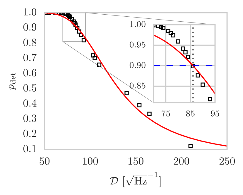
Figure 1: Detection probability $p_{\mathrm{det}}$ versus sensitivity depth $0pt$ for the S6-CasA-StackSlide-$\mathcal{F}$ search (cf. Table 2 and Sec. A.3), using a detection threshold of $2\overline{\mathcal{F}}_{\mathrm{th}}=8$. The squares indicate the results from a simulation in Gaussian noise, while the solid line gives the best-fit sigmoid of Eq. (59).

Another problem with this method is that the range of depths required to sample the relation $p_{\mathrm{det}}(0pt)$ often needs to be quite wide, due to initial uncertainties about where the UL value would be found, which can compound the above-mentioned sigmoid-fitting problem. Furthermore, the injection-recovery step can be quite computationally expensive, limiting the number of trials and further increasing the statistical uncertainty on the $p_{\mathrm{det}}$ measurements.

Both of these problems can be mitigated to some extent by using the sensitivity-estimation method described in this paper (Sec. III) to obtain a fairly accurate initial guess about the expected UL value, and then sample only in a small region around this estimate, in which case even a linear fit would probably yield good accuracy.

IV.2 Piecewise-linear threshold interpolation

An alternative approach is used in this work to obtain the simulated ULs: for each set of fixed-$0pt$ injections and recoveries, we determine the threshold on the statistic required in order to obtain the desired detection fraction $p_{\mathrm{det}}$. This is illustrated in Fig. 2, which shows a histogram of the observed loudest $2\overline{\mathcal{F}}$ candidates obtained in each of $N=10^{4}$ injection and recovery runs at a fixed signal depth of $0pt=$86\text{\,}\mathrm{Hz}^{-1/2}$$, using the S6-CasA-StackSlide-$\mathcal{F}$ search setup (cf. Sec. A.3). By integrating the probability density from $2\overline{\mathcal{F}}=0$ until we reach the desired value $1-p_{\mathrm{det}}$, we find the detection threshold $2\overline{\mathcal{F}}_{\mathrm{th}}$ at this signal depth $0pt$. Repeating this procedure at different depths therefore generates a sampling of the function $0pt^{p_{\mathrm{det}}}(2\overline{\mathcal{F}}_{\mathrm{th}})$, illustrated in Fig. 3. These points can be interpolated to the required detection threshold, which yields the desired upper-limit depth $0pt^{p_{\mathrm{det}}}$.

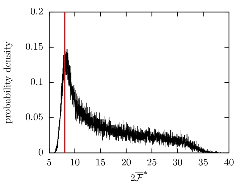
Figure 2: Histogram of recovered loudest $2\overline{\mathcal{F}}$ values for repeated searches on signal injections at fixed sensitivity depth $0pt=$86\text{\,}\mathrm{Hz}^{-1/2}$$ (with all other signal parameters randomized), using the search setup of the S6-CasA-StackSlide-$\mathcal{F}$ directed search. The vertical line indicates the resulting threshold value $2\overline{\mathcal{F}}_{\mathrm{th}}=7.995$ corresponding to $p_{\mathrm{det}}=90\,\%$ for this injection set.

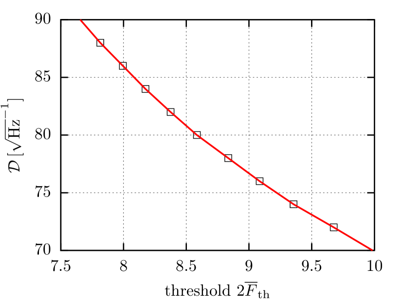
Figure 3: Sensitivity depth versus detection threshold. Boxes and solid lines indicate the piecewise-linear interpolation through the obtained thresholds at different depths of an injection-recovery simulation, using the S6-CasA-StackSlide-$\mathcal{F}$ search setup (Zhu et al. (2016) and Sec. A.3).

We see in in Fig. 3 that this function appears to be less “curvy” in the region of interest compared to $p_{\mathrm{det}}(0pt)$ shown in Fig. 1. This allows for easier fitting and interpolation, for example a linear or quadratic fit should work quite well. In fact, here we have simply used piecewise-linear interpolation, which is sufficient given our relatively fine sampling of signal depths.

As already mentioned in the previous section, using the sensitivity estimate of Sec. III one can determine the most relevant region of interest beforehand and focus the Monte-Carlo injection-recoveries on this region, which will help ensure that any simple interpolation method will work well.

Alternatively, for either the $p_{\mathrm{det}}(0pt)$- or the $0pt(2\mathcal{F}_{\mathrm{th}})$-sampling approach, one could also use an iterative root-finding method to approach the desired $p_{\mathrm{det}}$ or $2\mathcal{F}_{\mathrm{th}}$, respectively.

V Comparing estimates against simulated upper limits

In this section we compare the sensitivity estimates from Sec. III against simulated ULs for two example cases (an all-sky search and a directed search), in order to quantify the accuracy and reliability of the estimation method and implementation. This comparison shows generally good agreement, and also some instructive deviations.

Both examples are wide-parameter-space searches using a template bank over the unknown signal parameter dimensions (namely, {sky, frequency and spindown} in the all-sky case, and {frequency and first and second derivatives} in the directed-search case).

The simulated-UL procedure (see Sec. IV) performs a template-bank search over a box in parameter space containing the injected signal (at a randomized location) in Gaussian noise. On the other hand, the sensitivity estimate (cf. Eq. (45)) uses the mismatch distribution $P(\mu)$ obtained for this template bank via injection-recovery box searches on signals without noise. We refer to this in the following as the box search.

It will be instructive to also consider the (unrealistic) case of a perfectly-matched search, using only a single template that matches the signal parameters perfectly for every injection, corresponding to zero mismatch $\mu=0$ in Eq. (45). We refer to this as the zero-mismatch search.

V.1 Example: S6-AllSky-StackSlide-$\mathcal{F}$ search

In this example we use the setup of the all-sky search S6-AllSky-StackSlide-$\mathcal{F}$ Abbott et al. (2016d), which was using the GCT implementation Pletsch and Allen (2009) of the StackSlide-$\mathcal{F}$ statistic and was performed on the volunteer-computing project Einstein@Home Ein , see Table 1 and Sec. A.2 for more details.

Figure 4 shows the comparison between simulated ULs and estimated sensitivity depths $0pt^{90\%}$ versus threshold $2\overline{\mathcal{F}}_{\mathrm{th}}$, for the box search (squares and solid line), as well as for the zero-mismatch search (crosses and dashed line).

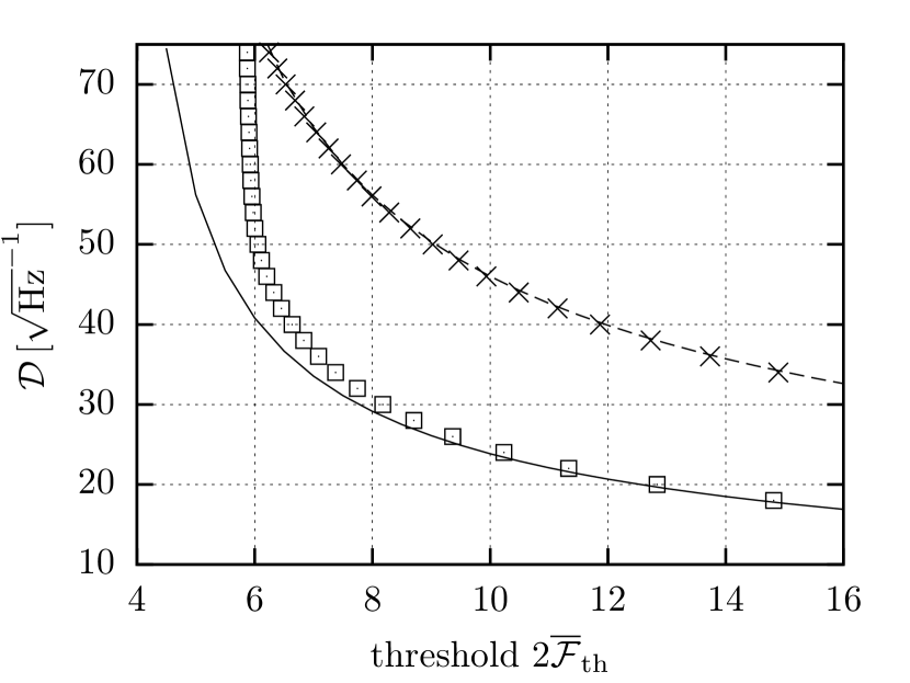
Figure 4: Comparison of estimated and simulated sensitivity depth $0pt^{90\%}$ as a function of threshold $2\overline{\mathcal{F}}_{\mathrm{th}}$ for the S6-AllSky-StackSlide-$\mathcal{F}$ search Abbott et al. (2016d). The solid line shows the UL estimate for the box search, and the squares ($\square$) show the corresponding simulated ULs. The dashed line indicates the estimate for the zero-mismatch case, and the crosses ($\times$) are for the simulated zero-mismatch ULs. In the box search we observe an increasing divergence at decreasing thresholds due to noise effects, discussed in Sec. V.1.

We see excellent agreement between estimated and simulated ULs for the zero-mismatch search. We also find very good agreement for the box-search at higher thresholds, while we see an increasing divergence $0pt\rightarrow\infty$ of the simulated ULs at decreasing thresholds, which is not captured by the estimate.

This discrepancy can be understood as the effect of noise fluctuations, which can enter in two different ways (that are not completely independent of each other):

1. For decreasing thresholds the corresponding false-alarm level Eq. (34) grows, as it becomes increasingly likely that a “pure noise” candidate (i.e. unrelated to a signal) crosses the threshold. In the extreme case where $p_{\mathrm{fa}}$ approaches $p_{\mathrm{det}}$, the frequentist upper limit would tend to $h_{0}\rightarrow 0$, corresponding to $0pt\rightarrow\infty$. This is illustrated in Fig. 5 showing the distribution of the loudest $2\overline{\mathcal{F}}$ in a box search on pure Gaussian noise, which can be compared to the diverging depth of the simulated box search around $2\overline{\mathcal{F}}_{\mathrm{th}}\lesssim 6$ in Fig. 4.

   

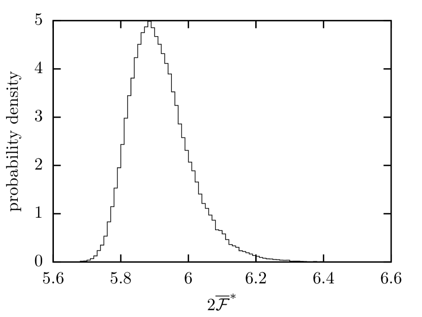
   Figure 5: Distribution of the loudest $2\overline{\mathcal{F}}$ for a box search on pure Gaussian noise, using the S6-AllSky-StackSlide-$\mathcal{F}$ search setup.

   We note that in practice the procedures used for measured ULs in CW searches typically make sure that the detection threshold has a very small false-alarm level, and we therefore expect this effect to have a negligible impact in cases of practical interest.

2. The sensitivity estimate for wide-parameter-space searches makes the assumption that the loudest candidate $2\overline{\mathcal{F}}^{*}$ is always found in the closest template to the signal (i.e. with the smallest mismatch $\mu$), as discussed in Sec. III.2. However, while the closest template has the highest expected statistic value (by definition), other templates can actually produce the loudest statistic value in any given noise realization. How likely that is to happen depends on the details of the parameter space, the template bank and the threshold. It will typically be more likely at lower thresholds, as more templates further away from the signal are given a chance to cross the threshold (despite their larger mismatch).

   The true distribution $P(2\overline{\mathcal{F}}^{*}\mid h_{0})$ of a box search will therefore be shifted to higher values compared to the approximate distribution used in Eq. (42). This implies that an actual search can have a higher detection probability than predicted by the estimate (corresponding to a larger sensitivity depth).

Both of these effects contribute to different extents to the box-search discrepancy in Fig. 4 at lower thresholds:

The sampling distribution for $2\overline{\mathcal{F}}^{*}$ in the presence of relatively strong signals at $0pt=$20\text{\,}\mathrm{Hz}^{-1/2}$$ is shown in Fig. 6, both for a simulated box search as well for the assumed distribution in the estimate.

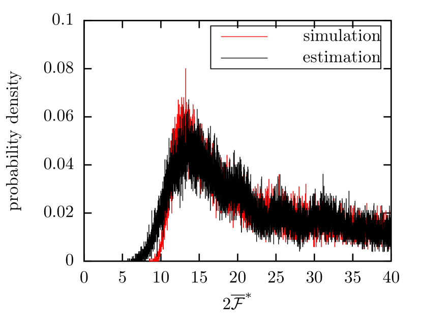
Figure 6: Loudest $2\overline{\mathcal{F}}$ distribution for a box-search (using the S6-AllSky-StackSlide-$\mathcal{F}$ setup) with signals at a depth of $0pt=$20\text{\,}\mathrm{Hz}^{-1/2}$$. The black histogram shows the assumed distribution for sensitivity estimation in Eq. (42), and the lighter color shows the histogram obtained in a Monte-Carlo simulation with signals injected in Gaussian noise.

We see that most of the loudest candidates obtained in the simulation are above $2\overline{\mathcal{F}}^{*}>9$, and are therefore extremely unlikely to be due to noise alone, as seen from Fig. 5. The difference between the two distributions in Fig. 6 is therefore soley due to effect (ii). However, we see in Fig. 4 that the resulting discrepancy in the sensitivity estimate at $0pt=$20\text{\,}\mathrm{Hz}^{-1/2}$$ is still very small.

For weaker signals at $0pt=$46\text{\,}\mathrm{Hz}^{-1/2}$$, we see in Fig. 7 that the corresponding distribution now overlaps with the pure-noise distribution of Fig. 5. The sensitivity depth therefore increasingly diverges for thresholds in the range $2\overline{\mathcal{F}}_{\mathrm{th}}\sim[5.8,6.1]$ due to the increasing impact of effect (i).

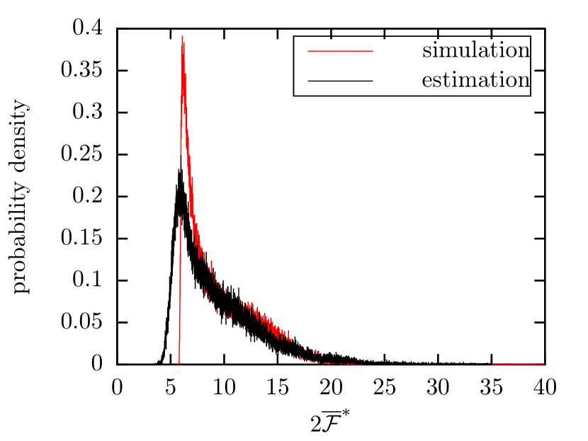
Figure 7: Same as Fig. 6 for weaker injected signals at a depth of $0pt=$46\text{\,}\mathrm{Hz}^{-1/2}$$.

V.2 Example: multi-directed O1-MD-StackSlide-$\mathcal{F}$

In this example we use the search setup of the directed search O1-MD-StackSlide-$\mathcal{F}$ Ming et al. (2018) currently running on Einstein@Home. This search consists of several directed searches for different targets on the sky, including Vela Jr. and Cas-A.

The comparison between simulated and estimated UL depths $0pt^{90\%}$ for these two targets is shown in Fig. 8.

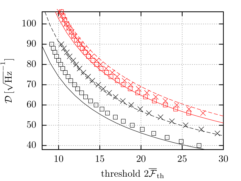
Figure 8: Comparison of estimated and simulated sensitivity depth $0pt^{90\%}$ as a function of the threshold $2\overline{\mathcal{F}}_{\mathrm{th}}$ for two targets of the multi-directed search setup O1-MD-StackSlide-$\mathcal{F}$. The solid lines show the UL estimate for a box search, while the squares ($\square$) show the corresponding simulated ULs. The dashed lines indicate the estimate for the zero-mismatch case, and the crosses ($\times$) are for the simulated zero-mismatch ULs. The upper group of curves are for the target Vela Jr., while the lower group of curves are for Cas A.

We see again very good agreement (relative deviations $\lesssim 3\%$) in the zero-mismatch case. However, these deviations are larger than in the all-sky case shown in Fig. 4. We suspect that this is due to the different antenna-pattern implementations of Eq. (70) between the search code and the estimation scripts: we see different signs of the deviation for different sky positions (Vela Jr. versus Cas-A), and the effect disappears when averaging over the whole sky (as seen in Fig. 4). However, the small size of the deviations did not warrant further efforts to try to mitigate this.

For the box-search case we see good agreement at higher thresholds, with again increasing deviations at lower thresholds due to the noise effects discussed in the previous all-sky example Sec. V.1.

VI Comparing estimates against measured upper limits

In this section we present a general overview of measured sensitivity depths $0pt_{\mathrm{meas}}$ derived from the published upper limits of various past CW searches. For the subset of searches where an $\mathcal{F}$-statistic-based method was used (and for Bayesian targeted ULs), we provide the sensitivity estimate for comparison.

The results are summarized in Tables 1– 4 for the different search categories (all-sky, directed and narrow-band, binary and targeted), and more details about each search are found in Appendix A.

VI.1 General remarks and caveats

VI.1.1 Bayesian UL comparison

We also provide sensitivity estimates (using the framework of Sec. III.6) for comparison to the Bayesian ULs of targeted searches for known pulsars (BayesPE), although these searches compute the $h_{0}$-posterior directly from the data rather than from an $\mathcal{F}$-statistic, which makes the comparison somewhat more indirect: we cannot use a known threshold or loudest candidate $2\mathcal{F}^{*}$, and we instead compute an expected depth by calculating estimates for $2\mathcal{F}^{*}$-values drawn randomly from the central $\chi^{2}_{4}$-distribution and averaging the results.

VI.1.2 Converting published $h_{0}$ ULs into Depths $0pt$

Some searches already provide their upper limits in the form of a sensitivity depth $0pt^{p_{\mathrm{det}}}$, but in most cases only the amplitude upper-limits $h_{0}^{p_{\mathrm{det}}}$ are given. For these latter cases we try to use a reasonable PSD estimate $S_{\mathrm{n}}(f)$ for the data used in the search in order to convert the quoted amplitude upper limits into sensitivity depths according to Eq. (33). This PSD estimate introduces a systematic uncertainty in the converted depth values, as in most cases we do not have access to the “original” PSD estimate used for the $h_{0}$ UL calculation.

In particular, even small differences in windowing or the type of frequency averaging can results in large differences in the PSD estimate near spectral disturbances. This can translate into large differences in the resulting converted depth values. In order to mitigate outliers due to such noise artifacts we quote the median over the converted measured depth values $\{0pt_{k}\}$ (where $k$ either runs over multiple frequencies, targets or detectors) and estimate the corresponding standard deviation using the mean absolute deviation (MAD) Rousseeuw and Croux (1993), namely

$$\begin{split}0pt^{\mathrm{med}}&\equiv\operatorname{median}\left[0pt_{k}\right]\,,\\ \widehat{\sigma}&\equiv 1.4826\,\operatorname{median}\left[\,\left|0pt_{k}-0pt^{\mathrm{med}}\right|\,\right]\,.\end{split}$$ (60)

VI.1.3 Comparing different searches by sensitivity depth $0pt$

We can see in the tables 1– 4 that searches within the same search category often show roughly comparable sensitivity depths. At one end of the spectrum are the fully-targeted searches, for which the parameter space (for each pulsar) is a single point, and one can achieve the maximal possible sensitivity for the available data, namely $0pt\sim\mathcal{O}\left($500\text{\,}\mathrm{Hz}^{-1/2}$\right)$ (see Table 5). At the other end of the spectrum lies the all-sky binary search with a sensitivity depth of $0pt\sim$3\text{\,}\mathrm{Hz}^{-1/2}$$ (see Table 4), which covers the largest parameter space of any search to date.

One cannot directly compare searches on sensitivity depth alone, even within the same search category. Other key aspects of a search are the parameter-space volume covered, the total computing power used, and the robustness of the search to deviations from the assumed signal- or noise-model.

Is it intuitively obvious that the more computing power spent on a fixed parameter-space volume, the more sensitive the search will tend to be, although the increase in sensitivity is typically very weak, often of order the 10th-14th root of the computing power Prix and Shaltev (2012).

It is also evident that the larger the parameter space covered by a search, the less sensitivity depth can be achieved due to the increased spending of computing power on “breadth” rather than depth. Ultimately the most directly relevant characteristic of a search would be its total detection probability Ming et al. (2016, 2018), which factors in both breadth and depth as well as the underlying astrophysical prior on signal amplitudes over the parameter space searched.

VI.2 All-sky searches

Estimated and measured sensitivity depths for all-sky searches are given in Table 1, and further details about individual searches can be found in appendix A.2.

Table 1: All-sky searches: estimated $0pt_{\mathrm{est}}$ and measured sensitivity depth $0pt_{\mathrm{meas}}$ (median and standard deviation, see Sec. VI.1.2). The columns labeled $f$ and $\dot{f}$ give the frequency and spindown ranges covered by each search. Sensitivity depths in italics refer to $90\%$-confidence upper limits, while normal font refers to $95\%$-confidence. See appendix A.2 for further details on the individual results.

Data	Search method	$f\,[$\mathrm{H}\mathrm{z}$]$	$\dot{f}\,[$\mathrm{nHz}\text{\,}{\mathrm{s}}^{-1}$]$	$0pt_{\mathrm{est}}\,[$\mathrm{Hz}^{-1/2}$]$	$0pt^{\mathrm{med}}_{\mathrm{meas}}\,[$\mathrm{Hz}^{-1/2}$]$	$\widehat{\sigma}_{0pt_{\mathrm{meas}}}\,[$\mathrm{Hz}^{-1/2}$]$	Ref, Sec
S2	Hough	[200, 400]	[-1.1, 0]	–	11.3	1.5	Abbott et al. (2005),A.2.1
S2	$\mathcal{F}$	[160, 728.8]	0	6.5	5.5	1.6	Abbott et al. (2007a),A.2.2
S4	StackSlide	[50, 1000]	[-10, 0]	–	10.5	1.1	Abbott et al. (2008a),A.2.3
S4	Hough	[50, 1000]	[-2.2, 0]	–	13.4	0.7	Abbott et al. (2008a),A.2.3
S4	PowerFlux	[50, 1000]	[-10, 0]	–	{6.1, 21.3}	{0.7, 2.3}	Abbott et al. (2008a),A.2.3
S4	$\mathcal{F}$+Coinc	[50, 1500]	[-9.5, 1]	–	8.5	0.5	Abbott et al. (2009),A.2.4
earlyS5	PowerFlux	[50, 1100]	[-5, 0]	–	{16.1, 47.9}	{2.4, 5.9}	Abbott et al. (2009),A.2.5
earlyS5	$\mathcal{F}$+Coinc	[50, 1500]	[-12.7, 1.3]	–	10.9	0.2	Abbott et al. (2009a),A.2.6
S5	PowerFlux	[50, 800]	[-6, 0]	–	{25.7, 71.3}	{0.7, 2.2}	Abadie et al. (2012),A.2.7
S5	Hough-$\mathcal{F}$	[50, 1190]	[-2, 0.1]	30.5	30.0	1.4	Aasi et al. (2013a),A.2.8
S5	Hough	[50, 1000]	[-0.9, 0]	–	28.1	0.6	Aasi et al. (2014b),A.2.9
S5	StackSlide-$\mathcal{F}$	[1249.7, 1499.7]	[-2.9, 0.6]	27.0	30.7	–	Singh et al. (2016),A.2.10
VSR1	$\mathcal{F}$TD+Coinc	[100, 1000]	[-16, 0]	–	22.6	6.0	Aasi et al. (2014a),A.2.11
VSR2,4	FreqHough+FUP	[20, 128]	[-0.1, 0.015]	–	35.5	11.1	Aasi et al. (2016),A.2.12
S6	StackSlide-$\mathcal{F}$	[50, 510]	[-2.7, 0.3]	34.4	37.0	–	Abbott et al. (2016d),A.2.13
S6	StackSlide-$\mathcal{F}$+FUP	[50, 510]	[-2.7, 0.3]	38.3	46.9	–	Papa et al. (2016),A.2.14
S6	PowerFlux	[100, 1500]	[-11.8, 10]	–	{17.9, 52.8}	{1.4, 3.4}	Abbott et al. (2016),A.2.15
O1	StackSlide-$\mathcal{F}$	[20, 100]	[-2.7, 0.3]	46.4	48.7	–	Abbott et al. (2017b),A.2.16
O1	PowerFlux	[20, 200]	[-10, 1]	–	28.9	2.2	Abbott et al. (2017b),A.2.17
O1	PowerFlux	[20, 475]	[-10, 1]	–	{19.9, 54.6}	{1.3, 3.2}	Abbott et al. (2017a),A.2.17
O1	SkyHough	[20, 475]	[-10, 1]	–	22.4	1.1	Abbott et al. (2017a),A.2.17
O1	$\mathcal{F}$TD+Coinc	[20, 475]	[-10, 1]	–	23.7	2.1	Abbott et al. (2017a),A.2.17
O1	FreqHough	[20, 475]	[-10, 1]	–	21.4	10.6	Abbott et al. (2017a),A.2.17
O1	PowerFlux	[475, 2000]	[-10, 1]	–	{18.6, 50.9}	{1.3, 3.4}	The LIGO Scientific Collaboration et al. (2018),A.2.17
O1	SkyHough	[475, 2000]	[-10, 1]	–	16.8	3.0	The LIGO Scientific Collaboration et al. (2018),A.2.17
O1	$\mathcal{F}$TD+Coinc	[475, 2000]	[-10, 1]	–	10.9	0.6	The LIGO Scientific Collaboration et al. (2018),A.2.17

The mean relative error between measured and estimated depths is $9\text{\,}\%$, while the median error is $7\text{\,}\%$.

One case of interest is the surprisingly large discrepancy of $\sim 18\%$ observed for the S6-AllSky-StackSlide-$\mathcal{F}$+FUP search, shown in Fig. 4, were we see a significantly higher measured depth ($0pt^{\mathrm{med}}_{\mathrm{meas}}=$46.9\text{\,}\mathrm{Hz}^{-1/2}$$) than estimated ($0pt_{\mathrm{est}}=$38.3\text{\,}\mathrm{Hz}^{-1/2}$$). This can be traced back to the template-maximization approximation used in the estimate, namely effect (ii) discussed in Sec. V.1. The low threshold used in the search ($2\overline{\mathcal{F}}_{\mathrm{th}}=6.1$) appears to be at the cusp of becoming affected by pure-noise candidates (effect (i) in Sec. V.1), but this effect is still small and does not account for the discrepancy. Furthermore, the upper limit procedure used a multi-stage follow-up, which ensures the final false-alarm level (p-value) is very small, which rules out contamination from pure-noise candidates.

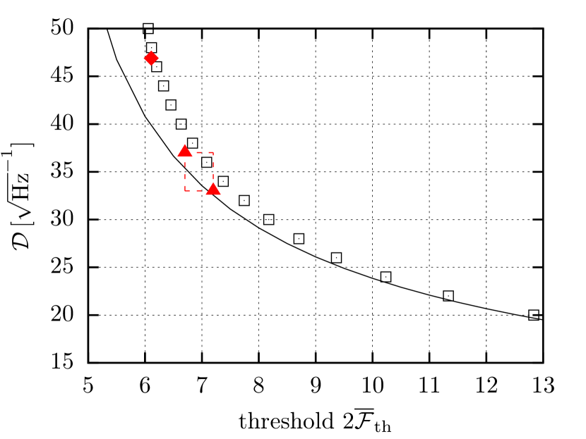
Figure 9: Estimated (–) and simulated ($\square$) sensitivity depth versus threshold $2\overline{\mathcal{F}}_{\mathrm{th}}$ for the S6-AllSky-StackSlide-$\mathcal{F}$ (+FUP) search setup, illustrating the effect of the template-maximization in the estimate (discussed in Sec. V.1). The triangles ($\Delta$) and dashed lines show the measured upper-limit depth $0pt^{\mathrm{med}}_{\mathrm{meas}}$ in the initial S6-AllSky-StackSlide-$\mathcal{F}$ search Abbott et al. (2016d), and the diamond ($\diamond$) shows the corresponding result from the follow-up (FUP) search Papa et al. (2016) (threshold $2\overline{\mathcal{F}}_{\mathrm{th}}=6.1$).

VI.3 Directed and Narrow-band searches

Estimated and measured sensitivity depths for directed and narrow-band searches are given in Tables 2 and 3, and further details about individual searches can be found in appendix A.3.

Table 2: Directed and narrow-band searches: estimated $0pt_{\mathrm{est}}$ and measured sensitivity depth $0pt_{\mathrm{meas}}$ (median and standard deviation, see Sec. VI.1.2). The column labeled $f$ gives the frequency range covered by each search (omitting $\dot{f}$ and $\ddot{f}$ search ranges). Sensitivity depths in italics refer to $90\%$-confidence upper limits, while normal font refers to $95\%$-confidence. See appendix A.3 for further details on the individual results.

Science run	Search method	Target	$f\,[$\mathrm{H}\mathrm{z}$]$	$0pt_{\mathrm{est}}\,[$\mathrm{Hz}^{-1/2}$]$	$0pt^{\mathrm{med}}_{\mathrm{meas}}\,[$\mathrm{Hz}^{-1/2}$]$	$\widehat{\sigma}_{0pt_{\mathrm{meas}}}\,[$\mathrm{Hz}^{-1/2}$]$	Ref, Sec
earlyS5	$\mathcal{F}$	Crab	59.56$\pm$0.006	221.3	223.1	–	Abbott et al. (2008b),A.3.1
S5	$\mathcal{F}$	CasA	[100, 300]	35.9	35.5	0.8	Abadie et al. (2010),A.3.2
S5	StackSlide-$\mathcal{F}$	GalacticCenter	[78, 496]	58.2	72.1	4.5	Aasi et al. (2013b),A.3.3
VSR4	5-vector	Vela	22.384$\pm$0.02	–	100.5	–	Aasi et al. (2015b),A.3.4
VSR4	5-vector	Crab	59.445$\pm$0.02	–	90.1	–	Aasi et al. (2015b),A.3.4
S6	$\mathcal{F}$	NineYoung (table 3)	[46, 2034]	37.8	37.7	0.3	Aasi et al. (2015a),A.3.5
S6	StackSlide-$\mathcal{F}$	CasA	[50, 1000]	79.6	72.9	0.4	Zhu et al. (2016),A.3.6
S6	LooselyCoherent	OrionSpur	[50, 1500]	–	{30.2, 85.7}	{2.3, 4.3}	Aasi et al. (2016),A.3.7
S6	$\mathcal{F}$	NGC6544	[92.5, 675]	29.3	29.6	1.7	Abbott et al. (2017a),A.3.8
O1	5-vector	11 pulsars	$<\pm 0.1$	–	111.6	12.2	Abbott et al. (2017d),A.3.9
O1	Radiometer	SN1987A	[25, 1726]	–	11.1	4.3	Abbott et al. (2017b),A.4.7
O1	Radiometer	GalacticCenter	[25, 1726]	–	7.7	2.9	Abbott et al. (2017b),A.4.7

The mean relative error between measured and estimated depths is $5\text{\,}\%$, and the median error is $1\text{\,}\%$.

Table 3: S6-NineYoung-$\mathcal{F}$ search: estimated $0pt_{\mathrm{est}}$ and measured sensitivity depth $0pt_{\mathrm{meas}}$ (median and standard deviation, see Sec. VI.1.2). for nine young supernova remnants Aasi et al. (2015a). All sensitivity depths refer to $95\%$-confidence. See appendix A.3.5 for further details.

SN remnant	G1.9	G18.9	G93.3	G111.7	G189.1	G266.2deep	G266.2wide	G291.0	G347.3	G350.1
Name			DA 530	Cas A	IC 443	Vela Jr.	Vela Jr.	MSH 11-62
$0pt_{\mathrm{est}}\,[$\mathrm{Hz}^{-1/2}$]$	$29.0$	$43.9$	$46.8$	$29.3$	$40.1$	$38.3$	$24.2$	$41.1$	$32.8$	$37.3$
$0pt^{\mathrm{med}}_{\mathrm{meas}}\,[$\mathrm{Hz}^{-1/2}$]$	$28.3$	$44.4$	$49.6$	$31.5$	$39.2$	$40.8$	$26.1$	$44.0$	$32.1$	$36.1$
$\widehat{\sigma}_{0pt_{\mathrm{meas}}}\,[$\mathrm{Hz}^{-1/2}$]$	$0.8$	$1.3$	$1.5$	$0.9$	$1.2$	$1.0$	$0.7$	$1.2$	$0.8$	$1.1$
$T_{\mathrm{data}}\,[${10}^{6}\text{\,}\mathrm{s}$]$	$1.2$	$3.1$	$2.8$	$1.1$	$2.3$	$1.9$	$0.7$	$2.2$	$1.4$	$1.9$
$2\mathcal{F}_{\mathrm{th}}$	$58.0$	$56.3$	$55.6$	$55.6$	$55.3$	$53.7$	$52.8$	$56.6$	$54.1$	$57.6$

For the S6-NineYoung-$\mathcal{F}$ search for nine young supernova remnants shown in Table 3, the mean relative error between measured and estimated depths is $4\text{\,}\%$ (median error $4\text{\,}\%$).

For two cases of interest we investigated more closely to understand the origin of the observed deviation:

S5-GalacticCenter-StackSlide-$\mathcal{F}$ search Aasi et al. (2013b): the reason for the relatively large deviation of $19\%$ in this case between $0pt_{\mathrm{est}}=$58.2\text{\,}\mathrm{Hz}^{-1/2}$$ and $0pt^{\mathrm{med}}_{\mathrm{meas}}=$72.1\text{\,}\mathrm{Hz}^{-1/2}$$ can be understood by looking at the details of this search setup: contrary to the assumed uniform averaging of antenna-pattern functions over time (cf. Sec. III.3, this search setup was specifically optimized by choosing the relatively short segments of $T_{\mathrm{seg}}=$11.5\text{\,}\mathrm{h}\mathrm{o}\mathrm{u}\mathrm{r}\mathrm{s}$$ in such a way as to maximize sensitivity, by selecting times of maximal antenna-pattern sensitivity towards the particular sky direction of the galactic center. This is described in more detail in Behnke et al. (2015), and is quoted there as yielding a sensitivity improvement of about $20\%$, consistent with the observed enhancement of measured sensitivity compared to our estimate.

S6-CasA-StackSlide-$\mathcal{F}$ search Zhu et al. (2016): the deviation between $0pt_{\mathrm{est}}=$79.6\text{\,}\mathrm{Hz}^{-1/2}$$ versus $0pt^{\mathrm{med}}_{\mathrm{meas}}=$72.9\text{\,}\mathrm{Hz}^{-1/2}$$ does not seem very large per se, but is unusual for the estimate typically does not tend to overestimate sensitivity by that much. A detailed investigation led us to discover a bug in the original upper-limit script used in Zhu et al. (2016), which resulted in the injection-recovery procedure to sometimes search the wrong box in parameter space, missing the injected signal. By artificially reproducing the bug in our upper limit simulation we are able to confirm that this bug does account for a decrease in detection probability of about $7\%$, resulting in an underestimate of the upper-limit depth as shown in Fig. 10.

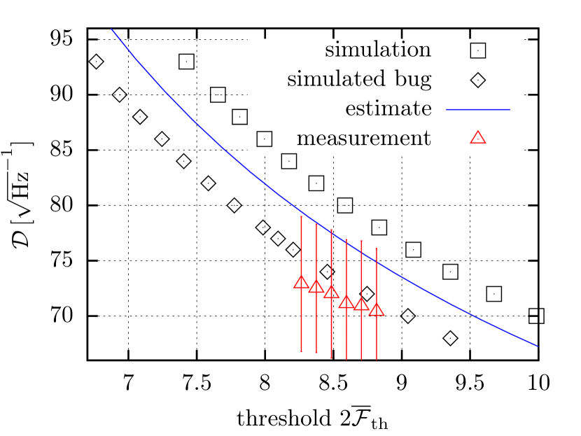
Figure 10: Estimated (–) and simulated ($\square$) sensitivity depth versus threshold $2\overline{\mathcal{F}}_{\mathrm{th}}$ for the S6-CasA-StackSlide-$\mathcal{F}$ search setup Zhu et al. (2016). The published upper limits are plotted as triangles ($\Delta$), while the diamonds ($\diamond$) show the simulated depths if we incorporate the bug found in the original UL procedure.

VI.4 Searches for neutron stars in binaries

Estimated and measured sensitivity depths for searches for CWs from neutron stars in binary systems are given in Tables 4, and further details about individual searches can be found in appendix A.4. In this case the only $\mathcal{F}$-statistic-based search is S2-ScoX1-$\mathcal{F}$, for which we obtain an estimate of $0pt_{\mathrm{est}}=$4.4\text{\,}\mathrm{Hz}^{-1/2}$$ (assuming an average mismatch of $\mu\sim 0.1/3$ corresponding to a cubic lattice with maximal mismatch of $0.1$ Abbott et al. (2007a)). The relative error is between measured and estimated sensitivity depth is therefore $8\text{\,}\%$.

Table 4: Binary searches: measured sensitivity depth $0pt_{\mathrm{meas}}$ (median and standard deviation, see Sec. VI.1.2). All sensitivity depths refer to $95\%$-confidence. See appendix A.4 for further details on the individual results.

Science run	Search method	Target	f [$\mathrm{H}\mathrm{z}$]	$0pt^{\mathrm{med}}_{\mathrm{meas}}\,[$\mathrm{Hz}^{-1/2}$]$	$\widehat{\sigma}_{0pt_{\mathrm{meas}}}\,[$\mathrm{Hz}^{-1/2}$]$	Ref, Sec
S2	$\mathcal{F}$	ScoX1	[464, 484],[604, 624]	4.1	0.1	Abbott et al. (2007a),A.4.1
S5	Sideband	ScoX1	[50, 550]	8.1	1.0	Aasi et al. (2015),A.4.2
S6,VSR2,3	TwoSpect	AllSky	[20, 520]	3.2	0.4	Aasi et al. (2014a),A.4.3
S6,VSR2,3	TwoSpect	ScoX1	[20, 57.25]	8.2	4.0	Aasi et al. (2014a),A.4.3
S6	TwoSpect	ScoX1	[40, 2040]	5.7	1.6	Meadors et al. (2017),A.4.4
S6	TwoSpect	J1751	{435.5, 621.5, 870.5}$\pm 1$	9.4	1.2	Meadors et al. (2017),A.4.4
O1	Viterbi	ScoX1	[60, 650]	7.6	1.0	Abbott et al. (2017f),A.4.5
O1	CrossCorr	ScoX1	[25, 2000]	24.0	2.0	Abbott et al. (2017e),A.4.6
O1	Radiometer	ScoX1	[25, 1726]	5.8	1.0	Abbott et al. (2017b),A.4.7

VI.5 Targeted searches for known pulsars

Estimated and measured sensitivity depths for targeted searches are given in Tables 5, and further details about individual searches can be found in appendix A.5.

Note that the quoted upper limits of the BayesPE-method are obtained by Bayesian parameter-estimation Dupuis and Woan (2005) of $P(h_{0}\mid x)$ directly on the data $x$. Therefore we cannot directly apply the Bayesian sensitivity estimate derived in Sec. III.6, which assumes an initial $\mathcal{F}(x)$-statistic computed on the data, from which the Bayesian upper limit would be derived. We therefore provide an approximate comparison with the expected sensitivity estimate, which we compute by estimating depths using $2\mathcal{F}^{*}$ drawn from a central $\chi^{2}_{4}$ distribution (given each target corresponds to a single template) and averaging the resulting estimated $0pt$ values. In cases where several targets are covered by the search, we assume for simplicity that the targets are isotropically distributed over the sky and compute a single all-sky sensitivity estimate. For single-target searches the exact sky position is used for the estimate.

Table 5: Targeted searches for known pulsars: estimated $0pt_{\mathrm{est}}$ and measured sensitivity depth $0pt_{\mathrm{meas}}$ (with respectively, median and standard deviation, see Sec. VI.1.1,VI.1.2). All sensitivity depths refer to $95\%$-confidence. See appendix A.5 for further details on the individual results.

Science run	Search method	Targets	$0pt^{\mathrm{med}}_{\mathrm{est}}\,[$\mathrm{Hz}^{-1/2}$]$	$\widehat{\sigma}_{0pt_{\mathrm{est}}}\,[$\mathrm{Hz}^{-1/2}$]$	$0pt^{\mathrm{med}}_{\mathrm{meas}}\,[$\mathrm{Hz}^{-1/2}$]$	$\widehat{\sigma}_{0pt_{\mathrm{meas}}}\,[$\mathrm{Hz}^{-1/2}$]$	Ref, Sec
S1	$\mathcal{F}$(worst-orientation)	J1939+21	70.8	39.8	64.2	38.1	Abbott et al. (2004),A.5.1
S1	$\mathcal{F}$	J1939+21	110.4	66.7	101.8	61.8	Abbott et al. (2004),A.5.1
S1	BayesPE	J1939+21	81.5	19.8	85.2	14.3	Abbott et al. (2004),A.5.1
S2	BayesPE	28 pulsars	243.5	54.3	156.4	42.2	Abbott et al. (2005),A.5.2
S3,4	BayesPE	78 pulsars	337.8	81.2	299.5	79.0	Abbott et al. (2007b),A.5.3
earlyS5	BayesPE	Crab	621.3	129.7	774.1	–	Abbott et al. (2008b),A.5.4
S5	BayesPE	116 pulsars	997.8	210.4	932.1	317.1	Abbott et al. (2010),A.5.5
VSR2	BayesPE,$\mathcal{F}$,5-vector	Vela	351.9	78.5	408.5	20.8	Abadie et al. (2011),A.5.6
S6,VSR2,4	BayesPE,$\mathcal{F}$,5-vector	195 pulsars	555.7	116.2	514.7	171.0	Aasi et al. (2014b),A.5.7
O1	BayesPE,$\mathcal{F}$,5-vector	200 pulsars	321.6	74.0	355.8	95.4	Abbott et al. (2017c),A.5.8

The mean relative error between measured and estimated depths is $16\text{\,}\%$, and the median error is $10\text{\,}\%$.

VII Discussion

In this paper we presented a fast and accurate sensitivity-estimation framework and implementation for $\mathcal{F}$-statistic-based search methods for continuous gravitational waves, extending and generalizing an earlier analytic estimate derived by Wette (2012). In particular the new method is more direct and uses fewer approximations for single-stage StackSlide-$\mathcal{F}$ searches, and is also applicable to multi-stage StackSlide-$\mathcal{F}$ searches, Hough-$\mathcal{F}$ searches and Bayesian upper limits (based on $\mathcal{F}$-statistic searches).

The typical runtime per sensitivity estimate is about $10\text{\,}\mathrm{s}\mathrm{e}\mathrm{c}\mathrm{o}\mathrm{n}\mathrm{d}\mathrm{s}$ with cached $P(R^{2})$ distribution, and about $25\text{\,}\mathrm{s}\mathrm{e}\mathrm{c}\mathrm{o}\mathrm{n}\mathrm{d}\mathrm{s}$ per detector for the first call with a new parameter prior. The accuracy compared to simulated Monte-Carlo upper limits in Gaussian noise is within a few $\%$ (provided the threshold corresponds to a low false-alarm level), and we find generally good agreement (of less than $\sim 10\%$ average error) compared to published upper limits in the literature. Several factors leading to the observed deviations in various cases are discussed in detail.

We also provided a comprehensive overview of published CW upper limit results, converting the quoted $h_{0}$ upper limits into sensitivity depths. This introduces some systematic uncertainties, as we often do not have access to the original PSD estimate used for the upper limits. We therefore advocate for future searches to directly provide their upper-limit results also in terms of the sensitivity depth of Eq. (33), in order to allow easier direct comparison between searches and to sensitivity estimates.

Appendix A Details on referenced CW searches

A.1 General remarks

In this appendix we will refer to the different detectors as G for GEO600 Grote (2010), V for VIRGO Accadia et al. (2012); Acernese et al. (2015), H1 and H2 for the two LIGO detectors in Hanford (4km, 2km) and L1 for LIGO Livingston Abbott et al. (2009b); Aasi et al. (2015).

We will use the common abbreviations CW for continuous gravitational waves, SFT for Short Fourier Transform, PSD for power spectral density and UL for upper limits.

The quoted sensitivity depths in tables 1 - 5 can correspond to different confidence levels, as some searches use $90\%$- and others $95\%$-confidence upper limits. This applicable confidence level is denoted by using regular versus italic font in the tables, respectively.

For searches over many frequencies, multiple targets or for upper limits reported separately for different detectors, we us a consistent averaging procedure using the median and median absolute deviation of Eq. (60) in order to estimate the mean and standard deviation in an outlier-robust way.

PowerFlux and loosely-coherent searches typically give separate upper limits for circular (best) polarisation and for the worst linear polarization, but not the more common type of population-averaged upper limits. There has been some work estimating conversion factors for these upper limits into into polarization-averaged sensitivity, writing $0pt^{\mathrm{PF}}\sim w_{\mathrm{worst}}0pt^{\mathrm{PF}}_{\mathrm{worst}}$ and $0pt^{\mathrm{PF}}\sim w_{\mathrm{best}}0pt^{\mathrm{PF}}_{\mathrm{best}}$. For example Wette (2012) obtains the conversion factors in the ranges $w_{\mathrm{worst}}\sim 1.1-1.3$ and $w_{\mathrm{best}}\sim 0.39-0.46$. More recent work estimating these conversion factors on O1 data (cf. Fig.Abbott et al. (2017b)) for $90\%$-confidence upper limits yields Dergachev (2018) $w_{\mathrm{worst}}1.51\pm 0.13$ and $w_{\mathrm{best}}=0.52\pm 0.02$. However, these conversion factors were obtained by treating the set of upper limits as a whole, they should not be used to derive a proxy of population average upper limits in individual frequency bands. Furthermore, PowerFlux strict upper limits are derived by taking the highest upper limits over regions of parameter space. This procedure has the advantage of the upper limits retaining validity over any subset of parameter space, such as a particular frequency and or particular sky location. However, the maximization procedure makes it difficult to convert the data into population average upper limits which are more robust to small spikes in the data. Given that there is currently some uncertainty on the detailed values of the conversion factors to use for different PowerFlux searches, here we report the best/worst upper limits converted into sensitivity depths separately in tables 1 and 2.

Generally, for converting $h_{0}$ upper limits into depths according to Eq. (33), we need to use an estimate for the corresponding noise PSD $S_{\mathrm{n}}$, for which we either use a corresponding PSD over the data used in the search, where available, or a ’generic’ PSD estimate from LIGO for the given science run iLI ; O1_ otherwise. This adds another level of uncertainty in the conversions, which could easily be in the range $10\%-20\%$ due to different calibrations and different types of averaging over time.

A.2 All-sky searches, see Table 1

A.2.1 S2-AllSky-Hough Abbott et al. (2005)

The first all-sky search for CWs from isolated neutron stars, using a semi-coherent Hough transform method applied on Short Fourier Transforms (SFTs) of the data of length $T_{\mathrm{seg}}=$30\text{\,}\mathrm{m}\mathrm{i}\mathrm{n}$$. The search used data from the second LIGO Science Run (S2), and the number of SFTs used in the search was $687$ from L1, $1761$ from H1 and $1384$ from H2.

The UL sensitivity depth for this search is calculated as the mean over the three depths for H1, L1 and H2, where each depth is computed from the respective quoted best upper-limit value $h_{0}^{95\%}$ and the corresponding PSD $S_{\mathrm{n}}$ in TABLE III of Abbott et al. (2005).

A.2.2 S2-AllSky-$\mathcal{F}$ Abbott et al. (2007a)

A matched-filtering search based on the coherent (single-detector) $\mathcal{F}$-statistics, using $20$ SFTs from H1 and $20$ SFTs from L1 (SFT length $T_{\mathrm{SFT}}=$30\text{\,}\mathrm{m}\mathrm{i}\mathrm{n}$$). The per-detector $\mathcal{F}$-statistic values were combined via a coincidence scheme, determining the most significant candidate in each $\sim$1\text{\,}\mathrm{H}\mathrm{z}$$ band, which was then used for measuring the upper limits.

The sensitivity depth for this search is calculated from the given (combined multi-detector) upper limits $h_{0}^{95\%}(f)$ over the search frequency range, combined with the harmonic mean over generic H1- and L1- PSDs for the LIGO S2 data.

The estimate was calculated with the mean loudest templates of the search given in the paper as $\mathcal{F}_{\mathrm{th}}=(39.5,32.2)$ for the L1 and H1 detector, respectively, and we used an average mismatch of $0.5\text{\,}\%$ in the H1 search and $1\text{\,}\%$ in the L1 search, estimated from Figs. 27,28 in Abbott et al. (2007a).

A.2.3 S4-AllSky-{StackSlide,Hough,PowerFlux}Abbott et al. (2008a)

Three semi-coherent all-sky searches using different search methods, all based on incoherently combining SFTs of length $T_{\mathrm{seg}}=$30\text{\,}\mathrm{m}\mathrm{i}\mathrm{n}$$. The StackSlide and the Hough search used $1004$ SFTs from H1 and $899$ from L1 and the Hough search additionally included $1063$ SFTs from H2. The PowerFlux search used $1925$ and $1628$ SFTs from H1 and L1, respectively.

The sensitivity depths are calculated from the quoted upper limits $h_{0}^{95\%}(f)$ from each of the three searches over the search frequency range, combined with the PSDs for two (H1 and L1) detectors (as a common reference) from the S4 science run. Note that the Hough depth corresponds to the quoted multi-detector UL, while the other searches reported only per-detector ULs.

A.2.4 S4-AllSky-$\mathcal{F}$+CoincAbbott et al. (2009)

A search which used the distributed computing project Einstein@Home Ein to analyse $300\text{\,}\mathrm{h}$ of H1 data and $210\text{\,}\mathrm{h}$ of L1 data from the S4 run. The data was split into $30\text{\,}\mathrm{h}$ long segments coherently analysed with the multi-detector $\mathcal{F}$-statistic followed by a coincidence-step. The measured sensitivity depth $0pt_{\mathrm{meas}}^{90\%}$ is calculated by converting the quoted sensitivity factors $R_{90\%}=\{31.8,33.2\}$ (for frequencies below and above $300\text{\,}\mathrm{H}\mathrm{z}$, respectively) into sensitivity depths. However, given these were computed with respect to an (arithmetic) averaged PSD estimate (given in Fig.1 in the paper), we first converted these factors back into equivalent $h_{0}$ values using the mean-PSD, and then computed the Depth with respect to the harmonic-mean (over detectors) generic noise PSD for S4.

A.2.5 earlyS5-AllSky-PowerFlux Abbott et al. (2009)

An all-sky search with PowerFlux over the first eight months of S5 data. The search in total used roughly $4077\text{\,}\mathrm{h}$ of H1 data and $3070\text{\,}\mathrm{h}$ L1 data, divided into SFT segments of $T_{\mathrm{seg}}=$30\text{\,}\mathrm{m}\mathrm{i}\mathrm{n}$$.

The sensitivity depth is calculated from the quoted per-detector upper limits $h_{0}^{95\%}(f)$ over the search frequency range and the corresponding S5 noise PSDs.

A.2.6 earlyS5-AllSky-$\mathcal{F}$+Coinc Abbott et al. (2009a)

An all-sky search run on Einstein@Home Ein , using $660\text{\,}\mathrm{h}$ of data from H1 and $180\text{\,}\mathrm{h}$ of L1 data, taken from the first 66 days of the LIGO S5 science run. The data was divided into $28$ segments of $T_{\mathrm{seg}}=$30\text{\,}\mathrm{h}$$ duration, and each segment was searched using the fully-coherent multi-detector $\mathcal{F}$-statistic. These per-segment $\mathcal{F}$-statistics were combined across segments using a coincidence scheme.

The measured sensitivity depth $0pt_{\mathrm{meas}}^{90\%}$ is calculated as the median over the converted sensitivity depths converted from the quoted sensitivity factors $R_{90\%}=\{29.4,30.3\}$ in the paper for the frequencies below and above $400\text{\,}\mathrm{H}\mathrm{z}$, respectively.

A.2.7 S5-AllSky-PowerFlux Abadie et al. (2012)

An all-sky search using PowerFlux analyzing the whole of LIGO S5 data, broken into more than $80\,000$ $50\,\%$-overlapping $30$-minute SFTs from both H1 and L1.

The sensitivity depth is calculated from the quoted upper limits $h_{0}^{95\%}$ and the S5 noise PSD.

A.2.8 S5-AllSky-Hough-$\mathcal{F}$ Aasi et al. (2013a)

An all-sky search using the Hough-$\mathcal{F}$ variant of the semi-coherent Hough method described in Sec. II.3.2, which was run on Einstein@Home. The analyzed data consisted of $5550$ and $5010$ SFTs from the LIGO H1 and L1 interferometers, respectively, taken from the second year of the S5 science run. The data was divided into $121$ segments of length $T_{\mathrm{seg}}=$25\text{\,}\mathrm{h}$$, and the coherent per-segment $\mathcal{F}$-statistic was combined via the Hough method to compute the Hough number count of Eq. (30).

The sensitivity depth of the search is calculated from the quoted $h_{0}^{90\,\%}$ upper limits and the corresponding S5 noise PSD.

The estimated sensitivity depth uses the generalization of the estimator described in Sec. III.5 with a number-count threshold of $n_{\mathrm{c,th}}=70$, a per segment threshold of $\tilde{\mathcal{F}}_{\mathrm{th}}=2.6$ and a mismatch histogram obtained from an injection-recovery simulation (with an average mismatch of $\tilde{\mu}=0.61$).

A.2.9 S5-AllSky-Hough Aasi et al. (2014b)

An SFT-based Hough all-sky search on S5 data. The search was split into the first and the second year of S5, which were searched separately. The first year used $11\,402$ SFTs from H1, $12\,195$ SFTs from H2 and $8\,698$ SFTs from L1, of length $T_{\mathrm{SFT}}=$30\text{\,}\mathrm{m}\mathrm{i}\mathrm{n}$$. The analysis of the second year used $12\,590$ H1-SFTs, $12\,178$ H2-SFTs and $10\,633$ L1-SFTs.

The sensitivity depth is calculated from the quoted $h_{0}^{90\%}$ upper limits of the second year search found in the paper and from the S5 noise PSD.

A.2.10 S5-AllSky-StackSlide-$\mathcal{F}$ Singh et al. (2016)

A high frequency all-sky search to complement previous lower-frequency all-sky searches on S5 data. The search used the so-called GCT method Pletsch and Allen (2009) implementing the StackSlide-$\mathcal{F}$ statistic and was run on the distributed Einstein@Home platform. The search used a total of $17\,797$ SFTs spanning the whole two years of S5 data from H1 and L1, divided into $205$ segments of length $T_{\mathrm{seg}}=$30\text{\,}\mathrm{h}$$.

The measured sensitivity depth $0pt_{\mathrm{meas}}^{90\%}$ is determined by extrapolating the depth values given in the paper for critical ratios of $0$ and $3.5$ to the median critical ratio over all frequency bands of $-0.15$ according to figure 6 of Singh et al. (2016).

For the estimate we determined the median threshold over all frequency bands from figure 4 of Singh et al. (2016) to $2\overline{\mathcal{F}}_{\mathrm{th}}=5.72$. Two mismatch histograms at $1255\text{\,}\mathrm{H}\mathrm{z}$ and $1495\text{\,}\mathrm{H}\mathrm{z}$ generated with injection-recovery studies were used. The average mismatch for both was $\mu\approx 0.82$. The quoted value is the mean of the two estimates with different mismatch histograms.

A.2.11 VSR1-AllSky-$\mathcal{F}$_TD+Coinc Aasi et al. (2014a):

An all-sky search using data from the first Virgo science run, VSR1. The search method uses a time-domain implementation of the coherent $\mathcal{F}$-statistic, computed over $2$-day coherent segments, which are combined using coincidences. In total the search used $134\text{\,}\mathrm{d}\mathrm{a}\mathrm{y}\mathrm{s}$ of data.

The measured sensitivity depth $0pt_{\mathrm{meas}}^{90\%}$ is calculated as median of the given sensitivity factors of $15.6$ and $22.4$.

A.2.12 {VSR2,4}-AllSky-FreqHough+FUP Aasi et al. (2016)

This all-sky search was performed using data from initial Virgos second (VSR2) and forth (VSR4) science run. It used the FrequencyHough transform as incoherent step with $149$ days of data of VSR2 and $476$ days of data of VSR4 using segments of length $8192\text{\,}\mathrm{s}\mathrm{e}\mathrm{c}\mathrm{o}\mathrm{n}\mathrm{d}\mathrm{s}$. The initial candidates were followed-up using $10$ times longer segments.

The measured sensitivity depth was calculated from upper limits $h_{0}^{90\%}$ extracted from figure 12 of Aasi et al. (2016) and the harmonic mean of the PSD estimates of VSR2 and VSR4 in $0.1\text{\,}\mathrm{H}\mathrm{z}$ frequency bands.

A.2.13 S6-AllSky-StackSlide-$\mathcal{F}$ Abbott et al. (2016d)

This search used $12\,080$ SFTs from L1 and H1 data to perform a StackSlide-$\mathcal{F}$ search based on the GCT implementation, and was run on Einstein@Home. The search used $90$ coherent segments of length $T_{\mathrm{seg}}=$60\text{\,}\mathrm{h}$$.

The measured sensitivity depth $0pt_{\mathrm{meas}}^{90\%}$ is determined by extrapolating the depth from the given critical ratios $0$ and $6$ to the median critical ratio of $-0.07$ according to figure 5 of Abbott et al. (2016d).

The estimated depth is given for a threshold of $2\overline{\mathcal{F}}_{\mathrm{th}}=6.694$ which is the median of the thresholds given for the frequency bands in figure 4 of Abbott et al. (2016d). For the estimate two mismatch histogram created with injection-recovery studies for $55\text{\,}\mathrm{H}\mathrm{z}$ and $505\text{\,}\mathrm{H}\mathrm{z}$ was used. The average mismatch of the grid in the parameter space was at both frequencies found to be $\mu=0.72$. The quoted value is the mean of the two estimates with different mismatch histograms.

A.2.14 S6-AllSky-StackSlide-$\mathcal{F}$+FUP Papa et al. (2016)

A multi-stage follow-up on candidates from the S6-AllSky-StackSlide-$\mathcal{F}$ search described in the previous paragraph, zooming in on candidates using increasingly finer grid resolution and longer segments. Every candidate from the initial stage with $2\overline{\mathcal{F}}\geq 6.109$ was used as the center of a new search box for the first-stage follow-up, continuing for a total of four semi-coherent follow-up stages. The sensitivity of the search is dominated by the initial-stage threshold, because the later stages are designed to have a very low probability of dismissing a real signal. The measured sensitivity depth $0pt_{\mathrm{meas}}^{90\%}=$46.9\text{\,}\mathrm{Hz}^{-1/2}$$ of this search is directly taken from the quoted value in the paper.

The estimated multi-stage sensitivity of Sec. III.4 using the thresholds given in the paper, namely $\{2\overline{\mathcal{F}}_{\mathrm{th}}^{(i)}\}=(6.109,6.109,7.38,8.82,15)$ and a mismatch histogram generated by recovery injection studies for the main search and mismatch histograms provided by the original authors for every stage with average mismatches $\{\mu^{(i)}\}=(0.72,0.55,0.54,0.29,0.14)$, yields a value of $0pt^{90\%}=$38.3\text{\,}\mathrm{Hz}^{-1/2}$$, which differs significantly from the quoted measured sensitivity depth. As discussed in Sec. V, we trace this discrepancy to the low threshold used, which significantly affects the loudest-candidate mismatch approximation used in the theoretical estimate.

A.2.15 S6-AllSky-PowerFlux Abbott et al. (2016)

The data used by this search span a time of $232.5\text{\,}\mathrm{d}$ with duty factor of the detectors of $53\%$ for H1 and $51\%$ for L1.

The measured sensitivity depth is calculated from the quoted upper limits $h_{0}^{95\%}$ in the paper and the S6 noise PSD.

A.2.16 O1-AllSky-StackSlide-$\mathcal{F}$ Abbott et al. (2017b)

A low-frequency all-sky search for gravitational waves from isolated neutron stars using the distributed computing project Einstein@Home on data from Advanced LIGO’s first observing run (O1). This search used the GCT implementation of the semi-coherent StackSlide-$\mathcal{F}$ method with $N_{\mathrm{seg}}=12$ segments of length $T_{\mathrm{seg}}=$210\text{\,}\mathrm{h}$$ in the initial search stage. The analyzed data consisted of $4\,744$ SFTs from the H1 and the L1 detector. The search also included a hierarchical follow-up similar to the S6Bucket follow-up searchPapa et al. (2016).

The measured sensitivity depth $0pt_{\mathrm{meas}}^{90\%}=$48.7\text{\,}\mathrm{Hz}^{-1/2}$$ of this search is directly taken from the quoted value in the paper.

The sensitivity estimate used a threshold $2\overline{\mathcal{F}}_{\mathrm{th}}=14.5$ which we inferred from figure 4 in Abbott et al. (2017b) and we obtained the mismatch histograms of the template grid at different frequencies using an injection-recovery study, which yielded an average mismatch of ${\mu}=0.35$ and ${\mu}=0.37$ at $20\text{\,}\mathrm{H}\mathrm{z}$ and $100\text{\,}\mathrm{H}\mathrm{z}$ respectively. The quoted depth is the average of the two different estimates resulting for each mismatch histogram. Note that the contrary to the measured sensitivity, the estimate only uses the first-stage parameters in this case, as we currently cannot model the line-robust statistic used in the follow-up stages. However, as mentioned in Sec. III.4, the overall detection probability is dominated by the first stage, while subsequent stages mostly serve to reduce the false-alarm level.

A.2.17 O1-AllSky-{PowerFlux,Hough,$\mathcal{F}$_TD+Coinc} Abbott et al. (2017a); The LIGO Scientific Collaboration et al. (2018)

Two papers detailing the results of all-sky searches on O1 data using four different search methods.

The first paper Abbott et al. (2017a) searched the lower frequency range $[20,475]\,\text{Hz}$, using four methods: PowerFlux, FrequencyHough, SkyHough and a time-domain $\mathcal{F}$-statistic search with segment-coincidences (denoted as $\mathcal{F}$_TD+Coinc). The PowerFlux, FrequencyHough and SkyHough search used SFT lengths in the range $1800-7200$\mathrm{s}$$ as coherent segments while the Time-Domain $\mathcal{F}$-statistic used a coherence time of $T_{\mathrm{seg}}=$6\text{\,}\mathrm{d}$$. The total amount of analyzed data was about $77\text{\,}\mathrm{d}$ of H1 data and $66\text{\,}\mathrm{d}$ of L1 data.

In the second paper The LIGO Scientific Collaboration et al. (2018) three of these searches were extended up to $2000\,\text{Hz}$, namely PowerFlux, SkyHough and a time-domain $\mathcal{F}$-statistic search with segment-coincidences (denoted as $\mathcal{F}$_TD+Coinc), using the same data.

The sensitivity depths for the four searches are calculated from the quoted $h_{0}^{95\%}$ amplitude upper limits and the noise PSD for the O1 science run.

Note that for the SkyHough method a sensitivity depth of $24.2\text{\,}\mathrm{Hz}^{-1/2}$ is quoted in the paper. However, this value is based on a slightly different convention for the multi-detector noise PSD $S_{\mathrm{n}}$ (maximum over detectors instead of the harmonic mean) than used here. For consistency with the other searches in table 1 we therefore compute the sensitivity depth by converting from the quoted $h_{0}^{95\%}$ upper limits instead.

A comparison of PowerFlux $90\%$-confidence upper limits for an isotropic polarization population were provided for the O1 Einstein@Home paper Abbott et al. (2017b), with a frequency spacing of $0.0625\text{\,}\mathrm{Hz}$, which are converted into sensitivity depth using the O1 noise PSD.

A.3 Directed Searches, see Tables 2, 3

A.3.1 earlyS5-Crab-$\mathcal{F}$ Abbott et al. (2008b)

This search aimed at the Crab pulsar and used the first nine month of initial LIGO’s fifth science run (S5). It consisted of both a targeted (described in Sec. A.5.4) and a directed $\mathcal{F}$-statistic search described here. The directed search used $182$, $206$ and $141$ days of data from the H1, H2 and L1 LIGO detectors, respectively. The measured depth value is calculated from the given upper limits $h_{0}^{95\%}$ and the PSD estimate of the S5 data at the search frequency.

The estimated depth uses the StackSlide estimator for a coherent search with $N_{\mathrm{seg}}=1$ segment, a threshold of $\mathcal{F}_{\mathrm{th}}=37$ and a maximal template bank mismatch of $5\%$ (given in the paper), from which we estimate the average mismatch as $\tilde{\mu}\sim\frac{1}{3}\,5\%$ (assuming a square lattice).

A.3.2 S5-CasA-$\mathcal{F}$ Abadie et al. (2010); Wette et al. (2008)

The first search for continuous gravitational waves from the Cassiopeia A supernova remnant using data from initial LIGO’s fifth science run (S5). The search coherently analyzed data in an interval of $12$ days ($934$ SFTs of length $30\text{\,}\mathrm{m}\mathrm{i}\mathrm{n}$) using the $\mathcal{F}$-statistic.

The measured sensitivity depth is obtained from the quoted upper limits $h_{0}^{95\%}$ in the paper and the S5 noise PSD.

The estimate is calculated using the StackSlide estimator for a coherent search ($N_{\mathrm{seg}}=1$ segment), with the mismatch histogram for an $A_{n}^{*}$ lattice with maximal mismatch of $\mu=0.2$ (obtained from LatticeMismatchHist() in Wette et al. (2018)), and the average threshold of $2\mathcal{F}_{\mathrm{th}}=55.8$ (averaged over the respective loudest $2\mathcal{F}$-candidates found in each of the upper-limit bands).

A.3.3 S5-GalacticCenter-StackSlide-$\mathcal{F}$ Aasi et al. (2013b); Behnke et al. (2015)

The first search for continuous gravitational waves directed at the galactic center. The search used LIGO S5 data and the GCT implementation of the StackSlide-$\mathcal{F}$ semi-coherent search algorithm with $630$ segments, each spanning $11.5\text{\,}\mathrm{h}$, for total data set of $21\,463$ SFTs of length $30\text{\,}\mathrm{m}\mathrm{i}\mathrm{n}$.

The segments of the search were selected from the whole S5 science run in such a way as to maximize the SNR for fixed-strength GW signals at the skyposition of the galactic center. Therefore the selected segments fall at times where the antenna patterns of the LIGO detectors are better than average for this particular skyposition. As discussed in Sec. VI.3, the sensitivity-estimation method presented in this work assumes the antenna patterns are averaged over multiple days, which causes a unusually large deviation between the estimate and the measured sensitivity depth from the $h_{0}^{90\%}$ upper limits.

The estimate is calculated using the mismatch histogram (with mean ${\mu}=0.13$) obtained from an injection-recovery study on the template bank of this search, and a detection threshold of $2\overline{\mathcal{F}}_{\mathrm{th}}=4.77$.

A.3.4 VSR4-{Vela,Crab}-5-vector Aasi et al. (2015b)

This coherent narrow-band search on the data from initial Virgo’s forth science run (VSR4) was directed at the Vela and the Crab pulsars. This search used the 5-vector method, and covers a range of $\pm$0.02\text{\,}\mathrm{H}\mathrm{z}$$ the twice the known frequencies of Vela and Crab. The total amount of data used is $76\text{\,}\mathrm{d}$.

The measured sensitivity depth for this search was obtained from the published $h_{0}^{95\%}$ upper limits and the noise PSD estimate for VSR4.

A.3.5 S6-NineYoung-$\mathcal{F}$ Aasi et al. (2015a)

This search was directed at nine different targets, listed in Table 3, each corresponding to a (confirmed or suspected) compact object in a young supernova remnant. The search uses a fully-coherent $\mathcal{F}$-statistic. The amount of data used for every target varies between $7.3\text{\times}{10}^{5}\text{\,}\mathrm{s}$ and $3.1\text{\times}{10}^{6}\text{\,}\mathrm{s}$ (cf. table 3).

The measured depth is calculated for each of the targets from the quoted upper limits $h_{0}^{95\%}$ and the corresponding PSD for the actual data used in the search.

The estimate for each target is calculated using the StackSlide estimator for a coherent search ($N_{\mathrm{seg}}=1$ segment), with the mismatch histogram for an $A_{n}^{*}$ lattice with maximal mismatch of $\mu=0.2$ (obtained from LatticeMismatchHist() in Wette et al. (2018)), and the average $2\mathcal{F}_{\mathrm{th}}$ threshold found for each target (averaged over the respective loudest $2\mathcal{F}$-candidates found in each of the upper-limit bands) are given in table 3.

The ’NineYoung’ entry in Table 2 presents the median depth over all targets for the measured and estimated depths, respectively.

A.3.6 S6-CasA-StackSlide-$\mathcal{F}$ Zhu et al. (2016)

A search directed at Cassiopeia A, which was run on the distributed computing project Einstein@Home using data from the LIGO S6 science run. The search was based on the GCT implementation of the semi-coherent StackSlide-$\mathcal{F}$ statistic, with $N_{\mathrm{seg}}=44$ segments of length $T_{\mathrm{seg}}=$140\text{\,}\mathrm{h}$$, and a total amount of data of $13\,143$ SFTs of length $30\text{\,}\mathrm{m}\mathrm{i}\mathrm{n}$ from the two LIGO detectors in Hanford (H1) and Livingston (L1). The measured sensitivity depth given in table 2 is computed from the $h_{0}^{90\%}$ upper limits quoted the paper Zhu et al. (2016) combined with the corresponding PSD estimates. However, as discussed in VI.3, this measurement suffered from a bug in the upper-limit script and as a result is somewhat too conservative (i.e. too high).

The estimated sensitivity is calculated assuming an average threshold of $\overline{\mathcal{F}}_{\mathrm{th}}=8.25$ (estimated from Fig. 4 in Zhu et al. (2016)) using the mean over estimates with different mismatch histograms generated by injection-recovery studies at different frequencies (spanning $50-1000\,\text{Hz}$, average mismatch $\sim 9\%$).

A.3.7 S6-OrionSpur-LooselyCoherent Aasi et al. (2016)

This was a search employing the so-called loosely-coherent method, aimed at the Orion spur towards both the inner and outer regions of our Galaxy. The explored sky regions are disks with $6.87\text{\,}{}^{\circ}$ diameter around $20^{h}10^{m}54.71^{s}+33^{\circ}33^{\prime}25.29^{\prime\prime}$ and $7.45\text{\,}{}^{\circ}$ diameter around $8^{h}35^{m}20.61^{s}-46^{\circ}49^{\prime}25.151^{\prime\prime}$. The data used in this search spanned $20\,085\,802\text{\,}\mathrm{s}$ with duty factors of $53\%$ and $51\%$ for LIGO Hanford and Livingston respectively. Due to weighting of the data the effective amount of data used was only $\sim 12.5\%$ of the available S6 data. For the analysis data segments of length $30\text{\,}\mathrm{m}\mathrm{i}\mathrm{n}$ were searched coherently.

The measured sensitivity depth was calculated from the quoted upper limits $h_{0}^{95\%}$ and a PSD estimate for the LIGO S6 data.

A.3.8 S6-NGC6544-$\mathcal{F}$ Abbott et al. (2017a)

This was the first search directed at the nearby globular cluster NGC 6544. The search coherently analyzed data from the two LIGO detectors S6 science run with the $\mathcal{F}$-statistic, using a single coherent segment with $T_{\mathrm{seg}}=$9.2\text{\,}\mathrm{d}$$. The search analyzed two different data stretches separately. The first one contained $374$ SFTs while the second contained $642$ SFTs, with SFT duration of $30\text{\,}\mathrm{m}\mathrm{i}\mathrm{n}$.

The measured depth was determined from the upper limits $h_{0}^{95\%}$ given in figure 2 of Abbott et al. (2017a) and a PSD estimate for the LIGO S6 run.

The estimate used the StackSlide estimator with one segment, a threshold of $2\mathcal{F}_{\mathrm{th}}=55$ (quoted in the paper) and an average mismatch of $0.2/3$ (assuming a roughly square lattice).

A.3.9 O1-Narrow-band-5-vectorAbbott et al. (2017d)

A narrow-band search aiming at 11 known pulsars using the fully-coherent 5-vector method on data from Advanced LIGO’s first observing run (O1). The search used a total of $121$ days of data from the Hanford (H1) and Livingston (L1) detectors.

The sensitivity depth in the table is calculated from the median over the single-target depths, which are converted from the upper-limits $h^{95\%}$ quoted in the paper and the corresponding noise PSD of the data used.

A.3.10 O1-{SN1987,GalacticCenter}-RadiometerAbbott et al. (2017b)

Described in Sec.A.4.7.

A.4 Searches for neutron stars in binary systems, see Table 4

A.4.1 S2-ScoX1-$\mathcal{F}$Abbott et al. (2007a)

This first search designed specifically aimed at the NS in the LMXB system Scorpius X-1, using a coherent single-detector $\mathcal{F}$-statistic and a coincidence check on a $6\text{\,}\mathrm{h}$ long stretch of S2 dat.

The measured sensitivity depth was calculated from the quoted upper limits $h_{0}^{95\%}$ in the paper (for the zero-eccentricity case $e=0$) and the PSD estimate of the corresponding S2 data.

A.4.2 S5-ScoX1-SidebandAasi et al. (2015)

A search aimed at Scorpius X-1 by incoherently combining sidebands of a coherent $\mathcal{F}$-statistic search that only demodulates the signal for the sky-position but not its binary-orbital Doppler modulation. This method used a stretch of $10$ days of data selected from the S5 science run for maximal sensitivity. Two searches were performed, one with no prior assumptions about the orientation of Sco-X1, and one using more restrictive angle-priors based on electromagnetic observations.

Bayesian upper limits $h_{0}^{95\%}$ were computed over the search frequency range, which we convert into sensitivity depths (for the unknown-polarization case, see Fig.5(a) in Aasi et al. (2015)) using the noise PSD for the data given in the paper. In each 1Hz-band, $2\times 10^{6}$ upper limit values were quoted, of which we use the maximum value in each 1Hz-band in order to be consistent with the usual “loudest-candidate” approach of setting upper limits in a given frequency band.

A.4.3 {S6,VSR2,3}-{AllSky,ScoX1}-TwoSpectAasi et al. (2014a)

A TwoSpect search for unknown binary signals from any sky-position, and a directed TwoSpect search for Scorpius X-1 specifically. This search used data from LIGO S6 science run, as well as from Virgo VSR2 and VSR3 runs, spanning $40\,551\,300\text{\,}\mathrm{s}$ from each detector.

The quoted upper limits $h_{0}^{95\%}$ for the all-sky search and the Scorpius X-1 search were converted into Depths using a combined (generic) PSD for the S6, VSR2 and VSR3 science runs.

A.4.4 S6-{ScoX1,J1751}-TwoSpectMeadors et al. (2017)

A search for CW from the low-mass X-ray binaries Scorpius X-1 and XTE J1751-305 using the TwoSpect algorithm. It used about $4\text{\times}{10}^{7}\text{\,}\mathrm{s}$ from each of the two detector in the S6 science run. It used two different length of the SFTs $840\text{\,}\mathrm{s}$ and $360\text{\,}\mathrm{s}$ which also where the length of the coherently analysed segments.

The given sensitivity depth $0pt_{0}^{95\%}$ is obtained from the quoted $h_{0}^{95\%}$ upper limits combined with the corresponding noise PSD for S6 data.

A.4.5 O1-ScoX1-ViterbiAbbott et al. (2017f)

A search aimed at Scorpius X-1 using the Viterbi search method performed on $130$ days of data from Advanced LIGO’s first observational run (O1), segmented into coherent segments of length $T_{\mathrm{seg}}=$10\text{\,}\mathrm{d}\mathrm{a}\mathrm{y}\mathrm{s}$$.

The measured sensitivity depth is converted from the quoted upper limits $h_{0}^{95\%}$ (for unknown polarization) and the noise PSD of the corresponding O1 data.

Note that contrary to many other search methods, this search setup appears to result in a frequency-dependent sensitivity depth, namely $0pt(f)\propto f^{-1/4}$ (see Eq.(9) in Abbott et al. (2017f)). For consistency with other searches, we quote the median and (MAD) standard-deviation over frequencies in Table 4, and note that the total range of sensitivity depths of this search is found as $0pt(f)\sim 11\,(f/f_{0})^{-1/4}\,$\mathrm{Hz}^{-1/2}$\in[4.6,11.2]\,$\mathrm{Hz}^{-1/2}$$ with $f_{0}=60.5\,\text{Hz}$.

A.4.6 O1-ScoX1-CrossCorrAbbott et al. (2017e)

This search aimed at Scorpius X-1 using the CrossCorr search algorithm using data from Advanced LIGO’s first observational run (O1). The data was split into coherently analysed segments (SFTs) with a (frequency-dependent) length between $240\text{\,}\mathrm{s}$ and $1400\text{\,}\mathrm{s}$.

The measured sensitivity depth is obtained from the quoted (isotropic-prior) upper limits $h_{0}^{95\%}$ and the noise PSD of the O1 data. Note, however, that the search ULs are given per $0.05\,\text{Hz}$ bands, which is unusually small compared to most other upper-limit bands (typically $0.25-1\,\text{Hz}$), and therefore they display more variability. In order to make these ULs more comparable to other searches, we use the 95th-percentile highest upper limits per 1Hz-bands (as recommended in Fig. 5 of Abbott et al. (2017e)). This ’binning’ procedure only has a small effect on the resulting sensitivity depth, which is reduced from $25.3\text{\,}\mathrm{Hz}^{-1/2}$ to $24.0\text{\,}\mathrm{Hz}^{-1/2}$.

Note that this search has a frequency-dependent sensitivity depth, which starts at around $0pt(25\,\text{Hz})\sim$45\text{\,}\mathrm{Hz}^{-1/2}$$ for low frequencies, asymptoting down to $0pt\sim$23\text{\,}\mathrm{Hz}^{-1/2}$$ above $f\gtrsim 800\,\text{Hz}$. However, in order to be consistent with other searches, we quote the median and (MAD) standard deviation over all frequencies in Table. 4.

A.4.7 O1-{ScoX1 and others}-RadiometerAbbott et al. (2017b)

The ’Radiometer’ search method, which was developed mainly for stochastic background searches, can also be used for directed CW searches at particular sky-positions. This method does not use a particular signal model, which allows it to be sensitive to a wide range of possible signal families, at the cost of somewhat lower sensitivity to ’regular’ CW signals. This search aimed at the sky-positions of Sco-X1, as well as at the supernova remnant 1987A and the galactic center.

The search reported $h_{0}^{90\%}$ (and $h_{0}^{95\%}$ for Sco-X1, reported in Abbott et al. (2017e)) upper limits in narrow frequency bands of $1/32\text{Hz}=0.03125\,\text{Hz}$ bands, which is unusually small compared to most other upper-limit bands (typically $0.25-1\,\text{Hz}$), and therefore they display more variability. In order to make these ULs more comparable to other searches, we use the 95th-percentile highest upper limits per 1Hz-bands (as recommended in Fig. 5 of Abbott et al. (2017e)), and following the same procedure as used for the CrossCorr results (discussed in Sec. A.4.6).

A.5 Targeted Searches, see Table 5

A.5.1 S1-J1939+21-{$\mathcal{F}$,BayesPE}Abbott et al. (2004)

This first CW search on data from GEO 600 and LIGO’s first science run (S1). It used $(16.7,5.73,8.73,8.9)$ days of data from four detectors, GEO 600 (G1), LIGO Livingston (L1), LIGO Hanford-$4\text{\,}\mathrm{k}\mathrm{m}$ (H1), and LIGO Hanford-$2\text{\,}\mathrm{k}\mathrm{m}$ (H2), respectively. Two types of searches were performed, a coherent $\mathcal{F}$-statistic search as well as direct Bayesian parameter estimation (BayesPE).

Table 5 gives the mean and standard deviation for the sensitivity depths over the four detectors. The measured sensitivity depth for the $\mathcal{F}$-search was determined from the quoted upper limits $h_{0}^{95\%}$ in table IVAbbott et al. (2004) for the most pessimistic $\iota$ ($\cos\iota=0$) and $\psi$, and from the quoted numbers in the conclusion for the (standard) population-averaged orientation. The noise PSD values are taken from table III in Abbott et al. (2004). The corresponding estimate is calculated with the StackSlide estimator for $N_{\mathrm{seg}}=1$ and quoted threshold values $2\mathcal{F}_{\mathrm{th}}=(1.5,3.6,6.0,3.4)$ for the four detectors from table III in the paper. For the ’worst-case’ estimate we use the prior $\cos\iota=0$ and minimise the sensitivity depth over $\psi\in[-\pi/4,\pi/4]$ in order to reflect the ’conservative’ ULs quoted in the paper. Note, however, that contrary to the typically small false-alarm level (p-value) of the UL thresholds used (typically $1\%$), the loudest candidates used here as thresholds here had relatively high p-values of $83\%$, $46\%$, $20\%$ and $49\%$, respectively, as seen in table III of Abbott et al. (2004).

A.5.2 S2-Known pulsars-BayesPEAbbott et al. (2005)

A coherent targeted search for $28$ known isolated radio pulsars was performed using the Bayesian parameter-estimation pipline (BayesPE) on data from the second LIGO Science Run (S2), using $910\text{\,}\mathrm{h}$ of data from H1, $691\text{\,}\mathrm{h}$ from H2 and $342\text{\,}\mathrm{h}$ of L1 data from the S2 data set.

The measured sensitivity depth is calculated from the quoted Bayesian upper limits $h_{0}^{95\%}$ and corresponding noise PSD estimates for the S2 science run.

The sensitivity estimate is performed using the Bayesian sensitivity estimator, for simplicity assuming the sources are distributed isotropically over the sky.

A.5.3 {S3,4}-Known pulsars-BayesPEAbbott et al. (2007b)

This search targeted $78$ known radio pulsars by analysing $(45.5,42.1,13.4)$ days of data from the three detectors (H1, H2, L1) from the third science run (S3) of LIGO and GEO 600, and $(19.4,22.5,17.1)$ days of data from the three detectors from the S4 science run. The analysis used the Bayesian parameter-estimation pipeline (BayesPE).

The measured sensitivity depth was determined from the quoted Bayesian upper limits $h_{0}^{95\%}$ combined with the noise PSD of the S3 and S4 science runs combined (using harmonic mean).

The sensitivity estimate is calculated using the Bayesian sensitivity estimate, for simplicity assuming the sources to be isotropically distributed on the sky.

A.5.4 earlyS5-Crab-BayesPEAbbott et al. (2008b)

This search on 9 months of data from the early LIGO S5 science run targeted only the Crab pulsar at twice its rotation rate, using the Bayesian parameter-estimation pipeline. A corresponding narrow-band search using the $\mathcal{F}$-statistic is described in Sec. A.3.1. The targeted search used $201$, $222$ and $158$ days of data of the H1, H2 and L1 LIGO detectors.

The measured depth is determined from the quoted (i.e. the corrected value in the Erratum) upper limit $h_{0}^{95\%}$ assuming an isotropic polarization prior, and the corresponding noise PSD of the detectors for the early S5 science run data.

A.5.5 S5-Known pulsars-BayesPEAbbott et al. (2010)

A search targeting 116 known pulsars using $525$ days of H1 data, $532$ days of H2 data and $437$ days of L1 data from LIGO’s fifth science run (S5). The search employed the Bayesian parameter-estimation pipeline.

The measured sensitivity depth is calculated from the quoted Bayesian upper limits $h_{0}^{95\%}$ and the noise PSD of the S5 data.

The estimate is calculated with the Bayesian sensitivity estimator under the assumption that the targets are distributed isotropically over the sky.

A.5.6 VSR2-Vela-{BayesPE,$\mathcal{F}$,5-vector}Abadie et al. (2011)

A targeted search for the Vela pulsar using Virgo’s second science-run (VSR2) data, using three different methods: Bayesian parameter estimation, the $\mathcal{F}$-statistic (and $\mathcal{G}$-statistic) and the 5-vector method. The data set consisted of $149$ days of Virgo data.

Two types of searches and upper limits were computed, namely (i) using uninformative (isotropic) priors on the pulsar orientation, and (ii) using angle priors on $\cos\iota$ and $\psi$ from electromagnetic observations.

In table 5 we only give the measured depth corresponding to the isotropic prior, averaged over the three methods, which obtained very similar results. This was computed from the quoted upper limits $h_{0}^{95\%}$ and the noise PSD for the Vela VSR2 run. The measured sensitivity depth obtained when using the angle priors is found as $462.1\pm 35.0\,$\mathrm{Hz}^{-1/2}$$.

The estimated sensitivity depth is calculated using the Bayesian sensitivity estimator.

A.5.7 {S6,VSR2,4}-Known pulsars-{BayesPE,$\mathcal{F}$,5-vector}Aasi et al. (2014b)

This search targeted 195 known pulsars, using $149$ days of VSR2 and $76$ days of VSR4 data for pulsars with a CW frequency lower than $f<$40\text{\,}\mathrm{H}\mathrm{z}$$ and an additional $238$ days of S6 data from H1 and $225$ days from L1 for faster spinning pulsars with $f>$40\text{\,}\mathrm{H}\mathrm{z}$$. The analysis was done using three different methods: Bayesian parameter estimation, the $\mathcal{F}$-statistic (or $\mathcal{G}$-statistic for restricted angle priors) and the 5-vector method.

The given measured sensitivity depth in table 5 is the median and MAD standard deviation over the sensitivity depths for the different targets (averaged over high- and low-frequency targets). The sensitivity depths are obtained from the quoted upper limits $h_{0}^{95\%}$ and the corresponding noise PSD estimate of the data used (which is either S6 and VSR2 and VSR4 for high-frequency targets $f>$40\text{\,}\mathrm{H}\mathrm{z}$$, or only VSR2 and VSR4 for low-frequency targets).

The estimated sensitivity is obtained from the Bayesian sensitivity estimator assuming an isotropic prior over the sky, averaged over high- and low-frequency depths results.

A.5.8 O1-Known pulsars-{BayesPE,$\mathcal{F}$,5-vector}Abbott et al. (2017c)

In this search $200$ known pulsars were targeted using three different methods: Bayesian parameter estimation, the $\mathcal{F}$-statistic (or $\mathcal{G}$-statistic for restricted angle priors) and the 5-vector method. The searches used $78$ and $66$ days of H1 and O1 data from the first observational run of advanced LIGO (O1), respectively.

The measured sensitivity depth is obtained from the quoted Bayesian upper limits $h_{0}^{95\%}$ over all targets and the corresponding noise PSD for the LIGO detectors during O1.

The estimated sensitivity depth is determined from the Bayesian estimator as an all-sky estimate assuming the targets are isotropically uniformly distributed over the sky.

Appendix B CW Signal model and $\mathcal{F}$-statistic

A plane gravitational wave arriving from a direction $\hat{n}$ (unit vector) can be written Bonazzola and Gourgoulhon (1996) in TT gauge (in the notation of Whelan et al. (2014)) as a purely spatial strain tensor $\tensor{h}$ with two polarizations $+,\times$, namely

$$\tensor{h}(\tau)=h_{+}(\tau)\,\tensor{e}_{+}+h_{\times}(\tau)\,\tensor{e}_{\times}\,,$$ (61)

where $\tau$ is the emission time of the signal in the source frame, and $\tensor{e}_{+}$ and $\tensor{e}_{\times}$ are the two polarization basis tensors, which can be constructed from a right-handed orthonormal basis $\{\hat{\ell},\hat{m},-\hat{n}\}$ as $\tensor{e}_{+}=\hat{\ell}\otimes\hat{\ell}-\hat{m}\otimes\hat{m}$ and $\tensor{e}_{\times}=\hat{\ell}\otimes\hat{m}+\hat{m}\otimes\hat{\ell}$.

The measured scalar CW signal $h^{X}(t)$ at time $t$ by detector $X$ is the response of the detector to the GW tensor $\tensor{h}(\tau^{X}(t))$, where $\tau^{X}(t)$ denotes the emission time of a wavefront that reaches detector $X$ at time $t$. This timing relationship depends on the sky-position $\hat{n}$ of the source as well as any binary-orbital parameters in case of a CW from a neutron star in a binary system, as it describes the time-dependent light-travel time from the source to the detector. In the long-wavelength limit we assume the GW wavelength to be much larger than the detector armlength, which is a good approximation for current ground-based detectors up to $\mathrm{kHz}$ frequencies. This allows us to write the detector response as a tensor contraction (in both tensor indices):

$$h^{X}(t)=\tensor{d}^{X}(t):\tensor{h}(\tau^{X}(t))\,,$$ (62)

where $\tensor{d}^{X}=\hat{u}\otimes\hat{u}-\hat{v}\otimes\hat{v}$ for interferometer arms along unit vectors $\hat{u}$ and $\hat{v}$.

It is helpful to define a source-independent orthonormal polarization basis $\{\hat{\imath},\hat{\jmath},-\hat{n}\}$ instead, where for any sky position $\hat{n}$, the unit vector $\hat{\imath}$ is chosen to lie in Earth’s equatorial plane (pointing West) and $\hat{\jmath}$ is pointing in the northern hemisphere. This defines the (sky-position dependent) alternative polarization basis as $\tensor{\varepsilon}_{+}(\hat{n})\equiv\hat{\imath}\otimes\hat{\imath}-\hat{\jmath}\otimes\hat{\jmath}$ and $\tensor{\varepsilon}_{\times}(\hat{n})\equiv\hat{\imath}\otimes\hat{\jmath}+\hat{\jmath}\otimes\hat{\imath}$. The rotation between these two basis systems defines the polarization angle $\psi$, which is measured counterclockwise from $\hat{\imath}$ to $\hat{\ell}$, and relates the two polarization basis tensors as

$$\tensor{e}_{+} =\hskip 6.99997pt\tensor{\varepsilon}_{+}\,\cos 2\psi+\tensor{\varepsilon}_{\times}\,\sin 2\psi\,$$ (63)

$$\tensor{e}_{\times} =-\tensor{\varepsilon}_{+}\,\sin 2\psi+\tensor{\varepsilon}_{\times}\,\cos 2\psi\,.$$ (64)

Combining these expression, we can obtain the factored signal form $h^{X}(t;\mathcal{A},\lambda)=\mathcal{A}^{\mu}\,h^{X}_{\mu}(t;\lambda)$ of Eq. (7), which was first derived in Jaranowski et al. (1998). The four amplitudes $\{\mathcal{A}^{\mu}\}_{\mu=1}^{4}$ depend on the signal amplitude $h_{0}$, the inclination angle $\iota$, polarization angle $\psi$, and the reference-time phase $\phi_{0}$, namely

$$\begin{split}\mathcal{A}^{1}&=\hskip 6.99997ptA_{+}\,\cos\phi_{0}\,\cos 2\psi-A_{\times}\,\sin\phi_{0}\,\sin 2\psi\,,\\ \mathcal{A}^{2}&=\hskip 6.99997ptA_{+}\,\cos\phi_{0}\,\sin 2\psi+A_{\times}\,\sin\phi_{0}\,\cos 2\psi\,,\\ \mathcal{A}^{3}&=-A_{+}\,\sin\phi_{0}\,\cos 2\psi-A_{\times}\,\cos\phi_{0}\,\sin 2\psi\,,\\ \mathcal{A}^{4}&=-A_{+}\,\sin\phi_{0}\,\sin 2\psi+A_{\times}\,\cos\phi_{0}\,\cos 2\psi\,,\end{split}$$ (65)

and the four (detector-dependent) basis functions $h_{\mu}^{X}(t;\lambda)$ are

$$\begin{split}h_{1}^{X}(t)&=a^{X}(t)\,\cos\phi(\tau^{X}(t))\,,\\ h_{2}^{X}(t)&=b^{X}(t)\,\cos\phi(\tau^{X}(t))\,,\\ h_{3}^{X}(t)&=a^{X}(t)\,\sin\phi(\tau^{X}(t))\,,\\ h_{4}^{X}(t)&=b^{X}(t)\,\sin\phi(\tau^{X}(t))\,,\end{split}$$ (66)

in terms of the antenna-pattern functions $a^{X}(t),b^{X}(t)$ given by the contractions

$$\begin{split}a^{X}(t;\hat{n})&=\tensor{d}^{X}(t):\tensor{\varepsilon}_{+}(\hat{n})\,,\\ b^{X}(t;\hat{n})&=\tensor{d}^{X}(t):\tensor{\varepsilon}_{\times}(\hat{n})\,.\end{split}$$ (67)

Using the factored signal form of Eq. (7), the log-likelihood ratio Eq. (68) now takes the form

$$\ln\Lambda(x;\mathcal{A},\lambda)=\mathcal{A}^{\mu}\,x_{\mu}-\frac{1}{2}\mathcal{A}^{\mu}\mathcal{M}_{\mu\nu}\mathcal{A}^{\nu}\,,$$ (68)

where we defined

$$x_{\mu}(\lambda)\equiv\left(x,h_{\mu}\right),\quad\text{and}\quad\mathcal{M}_{\mu\nu}(\lambda)\equiv\left(h_{\mu},h_{\nu}\right)\,,$$ (69)

in terms of the four basis function $h_{\mu}(t;\lambda)$ defined in Eq. (66). The $4\times 4$ antenna-pattern matrix $\mathcal{M}$ can be shown to be well approximated by the block-diagonal form

$$\mathcal{M}=S_{\mathrm{n}}^{-1}\,T_{\mathrm{data}}\,\begin{pmatrix}M&0\\ 0&M\\ \end{pmatrix}\;\text{with}\;M\equiv\begin{pmatrix}A&C\\ C&B\\ \end{pmatrix}\,,$$ (70)

defining the antenna-pattern coefficients $A,B,C$, which depend on the sky-position $\hat{n}$.

We see in Eq. (68) that the log-likelihood ratio is a quadratic function of the amplitudes $\mathcal{A}^{\mu}$, and can therefore be analytically maximized Jaranowski et al. (1998) (or marginalized Prix and Krishnan (2009)) to yield the well-known $\mathcal{F}$-statistic:

$$\begin{split}\mathcal{F}(x;\lambda)&\equiv\max_{\mathcal{A}}\ln\Lambda(x;\mathcal{A},\lambda)\\ &=\frac{1}{2}\,x_{\mu}\,\mathcal{M}^{\mu\nu}\,x_{\nu}\,,\end{split}$$ (71)

with $\mathcal{M}^{\mu\nu}$ defined as the inverse matrix to $\mathcal{M}_{\mu\nu}$ of Eq. (70).

Appendix C Distribution of $\mathcal{F}$-statistic maximized over correlated templates

It has been a long-standing assumption (e.g. Abadie et al. (2010); Wette (2012) that the distribution of the statistic $2\mathcal{F}^{*}(x)\equiv\max_{\lambda_{i}}2\mathcal{F}(x;\lambda_{i})$ in Gaussian noise $x$, maximized over a template bank $\lambda_{i}\in\mathbb{T}$ of $i=1\ldots\mathcal{N}$ (generally correlated) templates can be modelled by assuming maximization over an “effective” number of uncorrelated trials $\mathcal{N}^{\prime}$ instead, namely

$$P(2\mathcal{F}^{*}\mid\mathcal{N}^{\prime})=\mathcal{N}^{\prime}\,\operatorname{cdf}_{0}(2\mathcal{F}^{*})^{\mathcal{N}^{\prime}-1}\,\operatorname{pdf}_{0}(2\mathcal{F}^{*})\,,$$ (72)

where

$$\operatorname{pdf}_{0}(2\mathcal{F}) =P(2\mathcal{F}\mid\rho=0)\,,$$ (73)

$$\operatorname{cdf}_{0}(2\mathcal{F}) =\int_{0}^{2\mathcal{F}}\operatorname{pdf}_{0}(2\mathcal{F}^{\prime})\,\mathrm{\,d}2\mathcal{F}^{\prime}\,,$$ (74)

where the (single-template) $\mathcal{F}$-statistic in pure Gaussian noise follows a central $\chi^{2}$ distribution (with four degrees of freedom in the fully-coherent case Eq. (13), or $4N_{\mathrm{seg}}$ degrees of freedom for a semi-coherent $\mathcal{F}$-statistic over $N_{\mathrm{seg}}$ segments, Eq. (27)).

We show here by counter-example that the model of Eq. (72) is not generally accurate, as correlations between templates do not simply modify $\mathcal{N}^{\prime}$ but also change the functional form of the distribution. It has been hypothesized previously Wette (2012) that these (already-observed) deviations might be due to certain approximations (c.f. Prix (2010)) used in the numerical implementation of the $\mathcal{F}$ statistic. While such effects will account for some amount of deviation, one can show this effect to be quite small overall.

We demonstrate the fundamental statistical nature of this discrepancy by using a simpler example: we generate a time-series $\{x_{j}\}_{j=0}^{N-1}$ of $N=200$ samples drawn from a Gaussian distribution and compute the Fourier transform $\tilde{x}_{k}$ normalized to $E[|\tilde{x}_{k}|^{2}]=2$, such that $2\mathcal{F}_{2}(x,f)\equiv|\tilde{x}(f)|^{2}$ follows a central $\chi^{2}$ distribution with two degrees of freedom in every frequency bin $f$. We can therefore set $\operatorname{pdf}_{0}(2\mathcal{F}_{2})=\chi^{2}_{2}(2\mathcal{F}_{2};0)$ and use the corresponding cdf in Eq. (72).

We consider different cases of oversampling by zero-padding the time-series to a multiple (denoted as the oversampling factor in Fig. 11) of the original $N$ time samples: the $N/2-1=99$ (positive) frequency bins without oversampling are strictly uncorrelated (and we also know that there can be at most $N=200$ independent templates in total, given the length of the initial timeseries). With increasing oversampling, the correlations between frequency bins increase. We repeate this process $10^{6}$ times for different noise realizations, and in each case we compute $2\mathcal{F}^{*}_{2}(x)$ over all the (positive) frequency bins of the Fourier power, and histogram these values. We then fit the number of effective templates $\mathcal{N}^{\prime}$ in the theoretical distribution of Eq. (72) by minimizing the (symmetric) Jensen–Shannon divergence between the measured and theoretical distributions. The results are shown in Fig. 11 for different cases of oversampling.

(a)	(b)
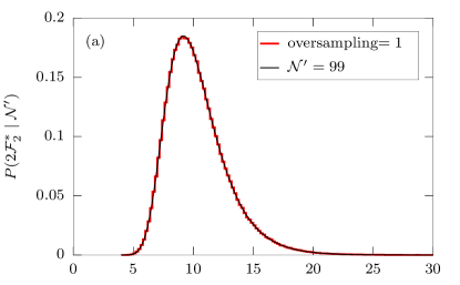
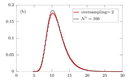
(c)	(d)

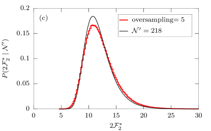
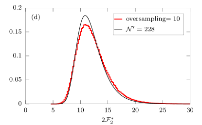
Figure 11: Stair-case plot: histogram (over $10^{6}$ repeated trials) of $2\mathcal{F}^{*}_{2}=\max_{k}|\tilde{x}_{k}|^{2}$ for Fourier transforms of Gaussian-noise timeseries, using different oversampling factors (a)–(d), where $\text{oversampling}=1$ corresponds to the original FFT frequency resolution. Solid thin line: corresponding best-fit theoretical model Eq. (72) with an effective number of templates $\mathcal{N}^{\prime}$.

We see that for increased oversampling, i.e. more correlations between ’templates’ (i.e. frequency bins), the functional form of the histogram agrees less with the theoretical distribution assuming independent templates. The effect seems to saturate for oversampling $\gtrsim 10$, with $\mathcal{N}\sim 230$ greater than the known maximal number (i.e. $N=200$ of (strictly) independent template in this vector space.

There is no simple or intuitive explanation for this effect that we are aware of, but it is reminiscent of a similarly surprising result found in the localization of the maximum over different assumed signal durations of transient CW signals, see Figs. 8 and 9 in Prix et al. (2011). The distribution of the statistic is identical in each time-step, but the steps are correlated, resulting in a peculiar non-uniform distribution of the location of the maximum.

References

- Wette (2012) Karl Wette, “Estimating the sensitivity of wide-parameter-space searches for gravitational-wave pulsars,” Phys. Rev. D. 85, 042003 (2012).
- Abbott et al. (2016a) B. P. Abbott, R. Abbott, T. D. Abbott, M. R. Abernathy, F. Acernese, K. Ackley, C. Adams, T. Adams, P. Addesso, R. X. Adhikari, et al., “Observation of Gravitational Waves from a Binary Black Hole Merger,” Phys. Rev. Lett. 116, 061102 (2016a), arXiv:1602.03837 [gr-qc] .
- Abbott et al. (2016b) B. P. Abbott et al. (LIGO Scientific Collaboration; Virgo Collaboration;), “Binary Black Hole Mergers in the first Advanced LIGO Observing Run,” Phys. Rev. X. 6 (2016b), 10.1103/PhysRevX.6.041015, arXiv:1606.04856 [gr-qc] .
- Abbott et al. (2017a) B. P. Abbott, R. Abbott, T. D. Abbott, F. Acernese, K. Ackley, C. Adams, T. Adams, P. Addesso, R. X. Adhikari, V. B. Adya, et al., “GW170817: Observation of Gravitational Waves from a Binary Neutron Star Inspiral,” Phys. Rev. Lett. 119, 161101 (2017a), arXiv:1710.05832 [gr-qc] .
- Abbott et al. (2016c) B. P. Abbott et al. (LIGO Scientific Collaboration; Virgo Collaboration), “Tests of general relativity with GW150914,” Phys. Rev. Lett. 116, 221101 (2016c), arXiv:1602.03841 [gr-qc] .
- Abbott et al. (2018a) B. P. Abbott et al. (The LIGO Scientific Collaboration; the Virgo Collaboration), “GW170817: Measurements of neutron star radii and equation of state,” ArXiv e-prints (2018a), arXiv:1805.11581 [gr-qc] .
- Abbott et al. (2017b) B. P. Abbott, R. Abbott, T. D. Abbott, F. Acernese, K. Ackley, C. Adams, T. Adams, P. Addesso, R. X. Adhikari, V. B. Adya, and et al., “A gravitational-wave standard siren measurement of the Hubble constant,” Nature 551, 85–88 (2017b), arXiv:1710.05835 .
- Prix (2009) Reinhard Prix, “Gravitational waves from spinning neutron stars,” in Neutron Stars and Pulsars (Springer, 2009) pp. 651–685.
- Lasky (2015) P. D. Lasky, “Gravitational Waves from Neutron Stars: A Review,” PASA 32, e034 (2015), arXiv:1508.06643 [astro-ph.HE] .
- Riles (2017) K. Riles, “Recent searches for continuous gravitational waves,” Modern Physics Letters A 32, 1730035-685 (2017), arXiv:1712.05897 [gr-qc] .
- Johnson-McDaniel and Owen (2013) N. K. Johnson-McDaniel and B. J. Owen, “Maximum elastic deformations of relativistic stars,” Phys. Rev. D. 88, 044004 (2013), arXiv:1208.5227 [astro-ph.SR] .
- Camenzind (2007) Max Camenzind, Compact objects in astrophysics: white dwarfs, neutron stars and black holes (Springer Science & Business Media, 2007).
- Knispel and Allen (2008) B. Knispel and B. Allen, “Blandford’s argument: The strongest continuous gravitational wave signal,” Phys. Rev. D. 78, 044031 (2008), 0804.3075 .
- Isi et al. (2017) M. Isi, M. Pitkin, and A. J. Weinstein, “Probing dynamical gravity with the polarization of continuous gravitational waves,” Phys. Rev. D. 96, 042001 (2017), arXiv:1703.07530 [gr-qc] .
- Abbott et al. (2018b) B. P. Abbott, R. Abbott, T. D. Abbott, F. Acernese, K. Ackley, C. Adams, T. Adams, P. Addesso, R. X. Adhikari, V. B. Adya, et al., “First Search for Nontensorial Gravitational Waves from Known Pulsars,” Phys. Rev. Lett. 120, 031104 (2018b), arXiv:1709.09203 [gr-qc] .
- Brady and Creighton (2000) P. R. Brady and T. Creighton, “Searching for periodic sources with LIGO. II. Hierarchical searches,” Phys. Rev. D. 61, 082001 (2000), gr-qc/9812014 .
- Prix and Shaltev (2012) R. Prix and M. Shaltev, “Search for continuous gravitational waves: Optimal StackSlide method at fixed computing cost,” Phys. Rev. D. 85, 084010 (2012), arXiv:1201.4321 [gr-qc] .
- Manchester et al. (2005) R. N. Manchester, G. B. Hobbs, A. Teoh, and M. Hobbs, “The australia telescope national facility pulsar catalogue,” The Astronomical Journal 129, 1993 (2005).
- Abbott et al. (2017c) B. P. Abbott, R. Abbott, T. D. Abbott, M. R. Abernathy, F. Acernese, K. Ackley, C. Adams, T. Adams, P. Addesso, R. X. Adhikari, et al., “First Search for Gravitational Waves from Known Pulsars with Advanced LIGO,” ApJ 839, 12 (2017c), arXiv:1701.07709 [astro-ph.HE] .
- Abbott et al. (2017d) B. P. Abbott, R. Abbott, T. D. Abbott, F. Acernese, K. Ackley, C. Adams, T. Adams, P. Addesso, R. X. Adhikari, V. B. Adya, et al., “First narrow-band search for continuous gravitational waves from known pulsars in advanced detector data,” Phys. Rev. D. 96, 122006 (2017d).
- Aasi et al. (2015a) J. Aasi, B. P. Abbott, R. Abbott, T. Abbott, M. R. Abernathy, F. Acernese, K. Ackley, C. Adams, T. Adams, P. Addesso, et al., “Searches for Continuous Gravitational Waves from Nine Young Supernova Remnants,” ApJ 813, 39 (2015a), arXiv:1412.5942 [astro-ph.HE] .
- Zhu et al. (2016) Sylvia J Zhu, Maria Alessandra Papa, Heinz-Bernd Eggenstein, Reinhard Prix, Karl Wette, Bruce Allen, Oliver Bock, David Keitel, Badri Krishnan, Bernd Machenschalk, et al., “Einstein@home search for continuous gravitational waves from cassiopeia a,” Phys. Rev. D. 94, 082008 (2016).
- Abbott et al. (2017e) B. P. Abbott, R. Abbott, T. D. Abbott, F. Acernese, K. Ackley, C. Adams, T. Adams, P. Addesso, R. X. Adhikari, V. B. Adya, et al., “Upper Limits on Gravitational Waves from Scorpius X-1 from a Model-based Cross-correlation Search in Advanced LIGO Data,” ApJ 847, 47 (2017e).
- Abbott et al. (2017f) B. P. Abbott, R. Abbott, T. D. Abbott, F. Acernese, K. Ackley, C. Adams, T. Adams, P. Addesso, R. X. Adhikari, V. B. Adya, et al., “Search for gravitational waves from Scorpius X-1 in the first Advanced LIGO observing run with a hidden Markov model,” Phys. Rev. D. 95, 122003 (2017f), arXiv:1704.03719 [gr-qc] .
- Abbott et al. (2017a) Benjamin P Abbott, R Abbott, TD Abbott, F Acernese, K Ackley, C Adams, T Adams, P Addesso, RX Adhikari, VB Adya, et al., “All-sky search for periodic gravitational waves in the o1 ligo data,” Phys. Rev. D. 96, 062002 (2017a).
- Abbott et al. (2017b) BP Abbott, R Abbott, TD Abbott, MR Abernathy, F Acernese, K Ackley, C Adams, T Adams, P Addesso, RX Adhikari, et al., “First low-frequency einstein@home all-sky search for continuous gravitational waves in advanced ligo data,” Phys. Rev. D. 96, 122004 (2017b).
- Goetz and Riles (2011) E Goetz and K Riles, “An all-sky search algorithm for continuous gravitational waves from spinning neutron stars in binary systems,” Class. Quant. Grav. 28, 215006 (2011).
- Aasi et al. (2014a) J Aasi, BP Abbott, Robert Abbott, T Abbott, MR Abernathy, T Accadia, F Acernese, K Ackley, C Adams, Thomas Adams, et al., “First all-sky search for continuous gravitational waves from unknown sources in binary systems,” Phys. Rev. D. 90, 062010 (2014a).
- Ming et al. (2016) J. Ming, B. Krishnan, M. A. Papa, C. Aulbert, and H. Fehrmann, “Optimal directed searches for continuous gravitational waves,” Phys. Rev. D. 93, 064011 (2016), arXiv:1510.03417 [gr-qc] .
- Ming et al. (2018) Jing Ming, Maria Alessandra Papa, Badri Krishnan, Reinhard Prix, Christian Beer, Sylvia J. Zhu, Heinz-Bernd Eggenstein, Oliver Bock, and Bernd Machenschalk, “Optimally setting up directed searches for continuous gravitational waves in Advanced LIGO O1 data,” Phys. Rev. D. 97, 024051 (2018).
- Leaci and Prix (2015) P. Leaci and R. Prix, “Directed searches for continuous gravitational waves from binary systems: parameter-space metrics and optimal Scorpius X-1 sensitivity,” Phys. Rev. D. 91, 102003 (2015), 1502.00914 .
- Abbott et al. (2004) B. Abbott, R. Abbott, R. Adhikari, A. Ageev, B. Allen, R. Amin, S. B. Anderson, W. G. Anderson, M. Araya, H. Armandula, et al., “Setting upper limits on the strength of periodic gravitational waves from PSR J1939+2134 using the first science data from the GEO 600 and LIGO detectors,” Phys. Rev. D. 69, 082004 (2004), gr-qc/0308050 .
- Krishnan et al. (2004) B. Krishnan, A. M. Sintes, M. A. Papa, B. F. Schutz, S. Frasca, and C. Palomba, “Hough transform search for continuous gravitational waves,” Phys. Rev. D. 70, 082001 (2004), gr-qc/0407001 .
- Mendell and Landry (2005) G. Mendell and M. Landry, StackSlide and Hough Search SNR and Statistics, Tech. Rep. (2005) lIGO Technical Document, LIGO-T050003-x0 .
- Abbott et al. (2008a) B Abbott, Robert Abbott, Rana Adhikari, Juri Agresti, P Ajith, Bruce Allen, R Amin, SB Anderson, WG Anderson, M Arain, et al., “All-sky search for periodic gravitational waves in ligo s4 data,” Phys. Rev. D. 77, 022001 (2008a).
- Aasi et al. (2013a) Junaid Aasi, J Abadie, BP Abbott, Richard Abbott, TD Abbott, Matthew Abernathy, Timothee Accadia, Fausto Acernese, Carl Adams, Thomas Adams, et al., “Einstein@home all-sky search for periodic gravitational waves in ligo s5 data,” Phys. Rev. D. 87, 042001 (2013a).
- Jaranowski et al. (1998) Piotr Jaranowski, Andrzej Krolak, and Bernard F Schutz, “Data analysis of gravitational-wave signals from spinning neutron stars: The signal and its detection,” Phys. Rev. D. 58, 063001 (1998).
- Finn (1992) Lee S. Finn, “Detection, measurement, and gravitational radiation,” Phys. Rev. D. 46, 5236–5249 (1992).
- Cutler and Schutz (2005) C. Cutler and B. F. Schutz, “Generalized F-statistic: Multiple detectors and multiple gravitational wave pulsars,” Phys. Rev. D. 72, 063006 (2005), gr-qc/0504011 .
- Prix (2007) R. Prix, “Search for continuous gravitational waves: Metric of the multidetector F-statistic,” Phys. Rev. D. 75, 023004 (2007), gr-qc/0606088 .
- Prix (2015) Reinhard Prix, The -statistic and its implementation in ComputeFstatistic_v2, Tech. Rep. (2015) (LIGO-T0900149-v5).
- Prix (2010) Reinhard Prix, “The F-statistic and its implementation in ComputeFStatistic v2,” LIGO-T0900149 (2010).
- Cutler et al. (2005) C. Cutler, I. Gholami, and B. Krishnan, “Improved stack-slide searches for gravitational-wave pulsars,” Phys. Rev. D. 72, 042004 (2005), gr-qc/0505082 .
- (44) “Einstein@home project page,” .
- Wette (2015) K. Wette, “Parameter-space metric for all-sky semicoherent searches for gravitational-wave pulsars,” Phys. Rev. D. 92, 082003 (2015), arXiv:1508.02372 [gr-qc] .
- Behnke et al. (2015) B. Behnke, M. A. Papa, and R. Prix, “Postprocessing methods used in the search for continuous gravitational-wave signals from the Galactic Center,” Phys. Rev. D. 91, 064007 (2015), arXiv:1410.5997 [gr-qc] .
- Abadie et al. (2010) J. Abadie, B. P. Abbott, R. Abbott, M. Abernathy, C. Adams, R. Adhikari, P. Ajith, B. Allen, G. Allen, E. Amador Ceron, et al., “First Search for Gravitational Waves from the Youngest Known Neutron Star,” ApJ 722, 1504–1513 (2010), arXiv:1006.2535 [gr-qc] .
- Wette et al. (2018) K. Wette, S. Walsh, R. Prix, and M. A. Papa, “Weave: a semicoherent search implementation for continuous gravitational waves,” ArXiv e-prints (2018), arXiv:1804.03392 [astro-ph.IM] .
- Miroslav Shaltev (2013) Reinhard Prix Miroslav Shaltev, “Fully coherent follow-up of continuous gravitational-wave candidates,” Phys. Rev. D. 87, 084057 (2013), arXiv:1303.2471 .
- Papa et al. (2016) M. A. Papa, H.-B. Eggenstein, S. Walsh, I. Di Palma, B. Allen, P. Astone, O. Bock, T. D. Creighton, D. Keitel, B. Machenschalk, R. Prix, X. Siemens, A. Singh, S. J. Zhu, and B. F. Schutz, “Hierarchical follow-up of subthreshold candidates of an all-sky Einstein@Home search for continuous gravitational waves on LIGO sixth science run data,” Phys. Rev. D. 94, 122006 (2016).
- Röver et al. (2011) C. Röver, C. Messenger, and R. Prix, “Bayesian versus frequentist upper limits,” in Proceedings of the PHYSTAT 2011 Workshop (2011) arXiv:1103.2987 [physics.data-an] .
- Dupuis and Woan (2005) R. J. Dupuis and G. Woan, “Bayesian estimation of pulsar parameters from gravitational wave data,” Phys. Rev. D. 72, 102002 (2005), gr-qc/0508096 .
- Eaton et al. (2015) John W. Eaton, David Bateman, Søren Hauberg, and Rik Wehbring, GNU Octave version 4.0.0 manual: a high-level interactive language for numerical computations (2015).
- Wette et al. (2018) Karl Wette, Reinhard Prix, David Keitel, Matthew Pitkin, Christoph Dreissigacker, John T. Whelan, and Paola Leaci, “OctApps: a library of Octave functions for continuous gravitational-wave data analysis,” Journal of Open Source Software 3, 707 (2018).
- Prix and Wette (2012) Reinhard Prix and Karl Wette, “Estimating sensitivity of the einstein@home search s5r5,” LIGO-T1200272 (2012).
- Abbott et al. (2016d) B. P. Abbott, R. Abbott, T. D. Abbott, M. R. Abernathy, F. Acernese, K. Ackley, C. Adams, T. Adams, P. Addesso, R. X. Adhikari, et al., “Results of the deepest all-sky survey for continuous gravitational waves on LIGO S6 data running on the Einstein@Home volunteer distributed computing project,” Phys. Rev. D. 94, 102002 (2016d), arXiv:1606.09619 [gr-qc] .
- Pletsch and Allen (2009) H. J. Pletsch and B. Allen, “Exploiting Large-Scale Correlations to Detect Continuous Gravitational Waves,” Phys. Rev. Lett. 103, 181102–+ (2009), 0906.0023 .
- Rousseeuw and Croux (1993) Peter J. Rousseeuw and Christophe Croux, “Alternatives to the median absolute deviation,” Journal of the American Statistical Association 88, 1273–1283 (1993), https://amstat.tandfonline.com/doi/pdf/10.1080/01621459.1993.10476408 .
- Abbott et al. (2005) B Abbott, R Abbott, R Adhikari, A Ageev, Juri Agresti, Bruce Allen, J Allen, R Amin, SB Anderson, WG Anderson, et al., “First all-sky upper limits from ligo on the strength of periodic gravitational waves using the hough transform,” Phys. Rev. D. 72, 102004 (2005).
- Abbott et al. (2007a) B. Abbott, R. Abbott, R. Adhikari, J. Agresti, P. Ajith, B. Allen, R. Amin, S. B. Anderson, W. G. Anderson, M. Arain, et al., “Searches for periodic gravitational waves from unknown isolated sources and Scorpius X-1: Results from the second LIGO science run,” Phys. Rev. D. 76, 082001 (2007a), gr-qc/0605028 .
- Abbott et al. (2009) B Abbott, Robert Abbott, Rana Adhikari, P Ajith, Bruce Allen, Gabrielle Allen, R Amin, DP Anderson, SB Anderson, WG Anderson, et al., “Einstein@home search for periodic gravitational waves in ligo s4 data,” Phys. Rev. D. 79, 022001 (2009).
- Abbott et al. (2009) B. P. Abbott, R. Abbott, R. Adhikari, P. Ajith, B. Allen, G. Allen, R. S. Amin, S. B. Anderson, W. G. Anderson, M. A. Arain, et al., “All-Sky LIGO Search for Periodic Gravitational Waves in the Early Fifth-Science-Run Data,” Phys. Rev. Lett. 102, 111102 (2009), 0810.0283 .
- Abbott et al. (2009a) BP Abbott, R Abbott, R Adhikari, P Ajith, B Allen, G Allen, RS Amin, SB Anderson, WG Anderson, MA Arain, et al., “Einstein@home search for periodic gravitational waves in early s5 ligo data,” Phys. Rev. D. 80, 042003 (2009a).
- Abadie et al. (2012) J Abadie, BP Abbott, Robert Abbott, TD Abbott, M Abernathy, T Accadia, F Acernese, C Adams, R Adhikari, C Affeldt, et al., “All-sky search for periodic gravitational waves in the full s5 ligo data,” Phys. Rev. D. 85, 022001 (2012).
- Aasi et al. (2014b) J Aasi, J Abadie, BP Abbott, R Abbott, T Abbott, MR Abernathy, T Accadia, F Acernese, C Adams, T Adams, et al., “Application of a hough search for continuous gravitational waves on data from the fifth ligo science run,” Class. Quant. Grav. 31, 085014 (2014b).
- Singh et al. (2016) A. Singh, M. A. Papa, H.-B. Eggenstein, S. Zhu, H. Pletsch, B. Allen, O. Bock, B. Maschenchalk, R. Prix, and X. Siemens, “Results of an all-sky high-frequency Einstein@Home search for continuous gravitational waves in LIGO’s fifth science run,” Phys. Rev. D. 94, 064061 (2016), arXiv:1607.00745 [gr-qc] .
- Aasi et al. (2014a) J. Aasi, B. P. Abbott, R. Abbott, T. Abbott, M. R. Abernathy, T. Accadia, F. Acernese, K. Ackley, C. Adams, T. Adams, et al., “Implementation of an F-statistic all-sky search for continuous gravitational waves in Virgo VSR1 data,” Class. Quant. Grav. 31, 165014 (2014a), arXiv:1402.4974 [gr-qc] .
- Aasi et al. (2016) J Aasi, BP Abbott, R Abbott, TD Abbott, MR Abernathy, F Acernese, K Ackley, C Adams, Thomas Adams, P Addesso, et al., “First low frequency all-sky search for continuous gravitational wave signals,” Phys. Rev. D. 93, 042007 (2016).
- Abbott et al. (2016) BP Abbott et al., “Comprehensive all-sky search for periodic gravitational waves in the sixth science run ligo data,” Phys. Rev. D. 94, 042002 (2016).
- The LIGO Scientific Collaboration et al. (2018) The LIGO Scientific Collaboration, the Virgo Collaboration, B. P. Abbott, R. Abbott, T. D. Abbott, F. Acernese, K. Ackley, C. Adams, T. Adams, P. Addesso, and et al., “Full Band All-sky Search for Periodic Gravitational Waves in the O1 LIGO Data,” Phys. Rev. D. 97, 102003 (2018), arXiv:1802.05241 [gr-qc] .
- Abbott et al. (2008b) B Abbott, Robert Abbott, Rana Adhikari, P Ajith, Bruce Allen, Gabrielle Allen, R Amin, SB Anderson, WG Anderson, MA Arain, et al., “Beating the spin-down limit on gravitational wave emission from the crab pulsar,” ApJL 683, L45 (2008b).
- Aasi et al. (2013b) Junaid Aasi, J Abadie, BP Abbott, Richard Abbott, Thomas Abbott, MR Abernathy, Timothee Accadia, Fausto Acernese, Carl Adams, Thomas Adams, et al., “Directed search for continuous gravitational waves from the galactic center,” Phys. Rev. D. 88, 102002 (2013b).
- Aasi et al. (2015b) J. Aasi, B. P. Abbott, R. Abbott, T. Abbott, M. R. Abernathy, F. Acernese, K. Ackley, C. Adams, T. Adams, T. Adams, et al., “Narrow-band search of continuous gravitational-wave signals from Crab and Vela pulsars in Virgo VSR4 data,” Phys. Rev. D. 91, 022004 (2015b), arXiv:1410.8310 [astro-ph.IM] .
- Aasi et al. (2016) J. Aasi, B. P. Abbott, R. Abbott, T. D. Abbott, M. R. Abernathy, F. Acernese, K. Ackley, C. Adams, T. Adams, P. Addesso, et al., “Search of the Orion spur for continuous gravitational waves using a loosely coherent algorithm on data from LIGO interferometers,” Phys. Rev. D. 93, 042006 (2016), arXiv:1510.03474 [gr-qc] .
- Abbott et al. (2017a) B. P. Abbott, R. Abbott, T. D. Abbott, M. R. Abernathy, F. Acernese, K. Ackley, C. Adams, T. Adams, P. Addesso, R. X. Adhikari, et al., “Search for continuous gravitational waves from neutron stars in globular cluster NGC 6544,” Phys. Rev. D. 95, 082005 (2017a), arXiv:1607.02216 [gr-qc] .
- Abbott et al. (2017b) B. P. Abbott, R. Abbott, T. D. Abbott, M. R. Abernathy, F. Acernese, K. Ackley, C. Adams, T. Adams, P. Addesso, R. X. Adhikari, and et al., “Directional Limits on Persistent Gravitational Waves from Advanced LIGO’s First Observing Run,” Phys. Rev. Lett. 118, 121102 (2017b), arXiv:1612.02030 [gr-qc] .
- Aasi et al. (2015) J Aasi, BP Abbott, R Abbott, T Abbott, MR Abernathy, F Acernese, K Ackley, C Adams, T Adams, P Addesso, et al., “A directed search for gravitational waves from scorpius x-1 with initial ligo data,” Phys. Rev. D. 91, 062008 (2015).
- Meadors et al. (2017) G. D. Meadors, E. Goetz, K. Riles, T. Creighton, and F. Robinet, “Searches for continuous gravitational waves from Scorpius X-1 and XTE J1751-305 in LIGO’s sixth science run,” Phys. Rev. D. 95, 042005 (2017), arXiv:1610.09391 [gr-qc] .
- Abbott et al. (2005) B. Abbott, R. Abbott, R. Adhikari, A. Ageev, B. Allen, R. Amin, S. B. Anderson, W. G. Anderson, M. Araya, H. Armandula, et al., “Limits on Gravitational-Wave Emission from Selected Pulsars Using LIGO Data,” Phys. Rev. Lett. 94, 181103 (2005), gr-qc/0410007 .
- Abbott et al. (2007b) B. Abbott, R. Abbott, R. Adhikari, J. Agresti, P. Ajith, B. Allen, R. Amin, S. B. Anderson, W. G. Anderson, M. Arain, et al., “Upper limits on gravitational wave emission from 78 radio pulsars,” Phys. Rev. D. 76, 042001 (2007b), gr-qc/0702039 .
- Abbott et al. (2010) B. P. Abbott, R. Abbott, F. Acernese, R. Adhikari, P. Ajith, B. Allen, G. Allen, M. Alshourbagy, R. S. Amin, S. B. Anderson, et al., “Searches for Gravitational Waves from Known Pulsars with Science Run 5 LIGO Data,” ApJ 713, 671–685 (2010), arXiv:0909.3583 [astro-ph.HE] .
- Abadie et al. (2011) Josh Abadie, BP Abbott, R Abbott, M Abernathy, T Accadia, F Acernese, C Adams, R Adhikari, C Affeldt, B Allen, et al., “Beating the spin-down limit on gravitational wave emission from the vela pulsar,” ApJ 737, 93 (2011).
- Aasi et al. (2014b) J. Aasi, J. Abadie, B. P. Abbott, R. Abbott, T. Abbott, M. R. Abernathy, T. Accadia, F. Acernese, C. Adams, T. Adams, et al., “Gravitational Waves from Known Pulsars: Results from the Initial Detector Era,” ApJ 785, 119 (2014b), arXiv:1309.4027 [astro-ph.HE] .
- Grote (2010) H. Grote (for the LIGO Scientific Collaboration), “The GEO 600 status,” Gravitational waves. Proceedings, 8th Edoardo Amaldi Conference, Amaldi 8, New York, USA, June 22-26, 2009, Class. Quant. Grav. 27, 084003 (2010).
- Accadia et al. (2012) T. Accadia et al. (VIRGO), “Virgo: a laser interferometer to detect gravitational waves,” Journal of Instrumentation 7, P03012 (2012).
- Acernese et al. (2015) F. Acernese et al. (VIRGO), “Advanced Virgo: a second-generation interferometric gravitational wave detector,” Class. Quant. Grav. 32, 024001 (2015), arXiv:1408.3978 [gr-qc] .
- Abbott et al. (2009b) B. P. Abbott et al. (LIGO Scientific Collaboration), “LIGO: The Laser interferometer gravitational-wave observatory,” Rept. Prog. Phys. 72, 076901 (2009b), arXiv:0711.3041 [gr-qc] .
- Aasi et al. (2015) J. Aasi et al. (LIGO Scientific Collaboration), “Advanced LIGO,” Class. Quant. Grav. 32, 074001 (2015).
- Dergachev (2018) Vladimir Dergachev, (2018), personal communication.
- (90) “Initial ligo strain noise data (psds),” .
- (91) “Representative O1 noise PSDs,” H1 LIGO-G1600150, L1 LIGO-G1600151.
- Wette et al. (2008) K. Wette, B. J. Owen, B. Allen, M. Ashley, J. Betzwieser, N. Christensen, T. D. Creighton, V. Dergachev, I. Gholami, E. Goetz, R. Gustafson, D. Hammer, D. I. Jones, B. Krishnan, M. Landry, B. Machenschalk, D. E. McClelland, G. Mendell, C. J. Messenger, M. A. Papa, P. Patel, M. Pitkin, H. J. Pletsch, R. Prix, K. Riles, L. Sancho de la Jordana, S. M. Scott, A. M. Sintes, M. Trias, J. T. Whelan, and G. Woan, “Searching for gravitational waves from Cassiopeia A with LIGO,” Class. Quant. Grav. 25, 235011 (2008), arXiv:0802.3332 [gr-qc] .
- Bonazzola and Gourgoulhon (1996) S. Bonazzola and E. Gourgoulhon, “Gravitational waves from pulsars: emission by the magnetic-field-induced distortion.” A&A 312, 675–690 (1996), astro-ph/9602107 .
- Whelan et al. (2014) J. T. Whelan, R. Prix, C. J. Cutler, and J. L. Willis, “New coordinates for the amplitude parameter space of continuous gravitational waves,” Class. Quant. Grav. 31, 065002 (2014), 1311.0065 .
- Prix and Krishnan (2009) R. Prix and B. Krishnan, “Targeted search for continuous gravitational waves: Bayesian versus maximum-likelihood statistics,” Class. Quant. Grav. 26, 204013–+ (2009), 0907.2569 .
- Prix et al. (2011) Reinhard Prix, Stefanos Giampanis, and Chris Messenger, “Search method for long-duration gravitational-wave transients from neutron stars,” Phys. Rev. D. 84, 023007 (2011), (eprint arXiv:1104.1704), arXiv:1104.1704 .