Coherent optical nano-tweezers for ultra-cold atoms

Abstract

There has been a recent surge of interest and progress in creating subwavelength free-space optical potentials for ultra-cold atoms. A key open question is whether geometric potentials, which are repulsive and ubiquitous in the creation of subwavelength free-space potentials, forbid the creation of narrow traps with long lifetimes. Here, we show that it is possible to create such traps. We propose two schemes for realizing subwavelength traps and demonstrate their superiority over existing proposals. We analyze the lifetime of atoms in such traps and show that long-lived bound states are possible. This work opens a new frontier for the subwavelength control and manipulation of ultracold matter, with applications in quantum chemistry and quantum simulation.

Coherent manipulation of atoms using light is at the heart of cold-atom-based quantum technologies such as quantum information processing and quantum simulation Gross and Bloch (2017); Lewenstein et al. (2012). The most commonly used methods to trap atoms optically are based on the AC Stark shift induced in a two-level system by an off-resonant laser field, which provides a conservative potential that is proportional to laser intensity. The spatial resolution of such a trapping potential is diffraction-limited, unless operated near surfaces González-Tudela et al. (2015); Mitsch et al. (2014); Thompson et al. (2013); Chang et al. (2009); Gullans et al. (2012); Romero-Isart et al. (2013). In contrast, a three-level system with two coupling fields offers more flexibility and can generate a subwavelength optical potential even in the far-field: although the intensity profiles of both laser beams involved are diffraction-limited, the internal structure of the state can change in space on length scales much shorter than the wavelength $\lambda$ of the lasers Agarwal and Kapale (2006); Bajcsy et al. (2003); Dutton et al. (2001); Gorshkov et al. (2008); Juzeliunas (2007); Miles et al. (2013); Sahrai et al. (2005); Yavuz and Proite (2007); Subhankar et al. (2018); Mcdonald et al. (2018). Such subwavelength internal-state structure can lead to subwavelength potentials either by creating spatially varying sensitivity to a standard AC Stark shift Yavuz et al. (2009) or by inducing a conservative subwavelength geometric potential Łacki et al. (2016); Jendrzejewski et al. (2016); Wang et al. (2018).

Trapping atoms in the far field on the subwavelength scale may allow for the realization of Hubbard-type models with increased tunneling and interaction energies Gullans et al. (2012); Romero-Isart et al. (2013); González-Tudela et al. (2015); Yi et al. (2008); Lundblad et al. (2008), which in turn would relax requirements on the temperature and coherence times in such experiments. Subwavelength traps can also be useful in atom-based approaches to quantum information processing Perczel et al. (2017); Grankin et al. (2018) and quantum materials engineering, as well as for efficient loading into traps close to surfaces González-Tudela et al. (2015); Mitsch et al. (2014); Thompson et al. (2013); Chang et al. (2009); Gullans et al. (2012); Romero-Isart et al. (2013). The use of dynamically adjustable subwavelength tweezers Barredo et al. (2016); Endres et al. (2016), in which atoms can be brought together and apart, can also enable controlled ultracold quantum chemistry Dirk-Sören Lühmann et al. (2015); Ospelkaus et al. (2010); Liu et al. (2018).

To trap atoms on a subwavelength scale, the optical potential must provide a local minimum. The geometric scalar potential associated with laser-induced internal-state structure is always repulsive and increases in magnitude as its spatial extent is reduced. This repulsive contribution must be considered when engineering attractive subwavelength optical potentials. A trap based on the combination of AC Stark shift and subwavelength localization Gorshkov et al. (2008); Bajcsy et al. (2003); Dutton et al. (2001); Sahrai et al. (2005); Agarwal and Kapale (2006); Yavuz and Proite (2007); Juzeliunas (2007); Miles et al. (2013); Kapale (2013); Johnson et al. (1998); Thomas (1989); Stokes et al. (1991); Schrader et al. (2004); Gardner et al. (1993); Zhang et al. (2006); Lee et al. (2007); Kapale and Agarwal (2010); Le Kien et al. (1997); Qamar et al. (2000); Paspalakis and Knight (2001); Hell (2007); Li et al. (2008); Mompart et al. (2009); Sun et al. (2011); Proite et al. (2011); Qi et al. (2012); Viscor et al. (2012); Yavuz and Simmons (2012); Rubio et al. (2013) within a three-level system was proposed in Ref. Yavuz et al. (2009), but the geometric potentials arising from non-adiabatic corrections to the Born-Oppenheimer approximation Łacki et al. (2016); Jendrzejewski et al. (2016) were not considered. In this Letter, we show that even with the repulsive non-adiabatic corrections, attractive subwavelength potentials are still possible. We also propose two alternative schemes for the generation of traps that offer significantly longer trapping times as compared to the approach of Ref. Yavuz et al. (2009). We analyze the performance of all three approaches and show that 8nm-wide traps offering 10ms trapping times are within reach. Compared with near-field methods, our far-field approach not only avoids losses and decoherence mechanisms associated with proximity to surfaces, but also provides more flexibility in time-dependent control of the shape and position of the trapping potentials and, additionally, works not only in one and two but also in three dimensions.

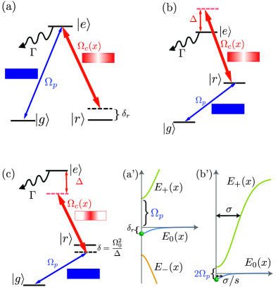
Figure 1: (a) Level diagram for the EIT scheme, showing a spatially homogeneous field $\Omega_{p}$ [blue bar] and a spatially varying field $\Omega_{c}(x)=\Omega_{0}(1-e^{-x^{2}/\sigma^{2}})^{1/2}$ [red bar with gradient]. $\Gamma$ is the linewidth of the excited state. (b) Level diagram for the blue-detuned AC-Stark scheme. The intermediate state $\ket{r}$ is dressed by coupling it to the excited state $\ket{e}$ with a spatially dependent $\Omega_{c}(x)=\Omega_{0}(1-e^{-x^{2}/\sigma^{2}})^{1/2}$ and a large detuning $\Delta\gg\Omega_{c}$, which gives rise to a light-shift $\Omega^{2}_{c}(x)/\Delta$ of state $\ket{r}$. The ground state $\ket{g}$ is coupled to state $\ket{r}$ with a spatially uniform $\Omega_{p}$ and detuning $\delta=0$. (c) Level diagram for the red-detuned AC-Stark scheme Yavuz et al. (2009). The difference from (b) is that $\Omega_{c}(x)=\Omega_{0}e^{-x^{2}/(2\sigma^{2})}$ is maximal at $x=0$ and that $|\Delta|\gg\Omega_{c},\delta$ now indicates the amount of red detuning. Moreover, the detuning $\delta=\Omega^{2}_{0}/\Delta$ is chosen to exactly compensate for the light-shift of $\ket{r}$ at $x=0$. (a’,b’) Sketches of the relevant eigenstates (atom depicted by a green ball is trapped in the blue potential): (a’) for the (a) scheme; (b’) for the (b) scheme, which for $x<w$ is equivalent to the (c) scheme. Although $E_{\pm}$ are diffraction limited, $E_{0}$ has subwavelength shape characterized by width $w$, which can be expressed using the enhancement factor defined as $s=\sigma/w$.

Model.—We start with a single-atom Hamiltonian

$$H=H_{\rm\scriptscriptstyle al}(x)+\frac{p^{2}}{2m},$$ (1)

where $m$ is the mass, $p$ is the momentum, and $H_{\rm\scriptscriptstyle al}$ describes the atom-light interaction. We will consider three schemes shown in Fig. 1: (a) electromagnetically induced transparency (EIT), (b) blue-detuned AC-Stark, and (c) red-detuned AC-Stark Yavuz et al. (2009). For the EIT scheme ($\hbar=1$),

$$H_{\rm\scriptscriptstyle al}=\left(\begin{array}[]{ccc}\delta_{r}&0&\Omega_{c}(x)\\ 0&0&\Omega_{p}\\ \Omega_{c}(x)&\Omega_{p}&\Delta\\ \end{array}\right)$$ (5)

in the basis of bare atomic states $\{\ket{r},\ket{g},\ket{e}\}$, where $2\Omega_{p}$ and $2\Omega_{c}(x)$ are Rabi frequencies of a spatially homogeneous probe field and a spatially-varying control field, respectively. For the two AC-Stark schemes, in the limit of large single-photon detuning $|\Delta|\gg\Omega_{c}(x),\Omega_{p},|\delta|$ [see Fig. 1(b,c)], the intermediate state $\ket{e}$ can be adiabatically eliminated, resulting in an effective two-state Hamiltonian

$$H_{\rm\scriptscriptstyle al}=\left(\begin{array}[]{cc}\delta-\frac{\Omega_{c}^{2}(x)}{\Delta}&\Omega_{p}\\ \Omega_{p}&0\end{array}\right)$$ (8)

in the $\{\ket{r},\ket{g}\}$ basis.

Within the Born-Oppenheimer approximation, we first diagonalize $H_{\rm\scriptscriptstyle al}$ which leads to position-dependent eigenstates. Non-adiabatic corrections give rise to geometric scalar $U$ and vector ${A}$ potentials, defined as $U=R^{\dagger}\partial_{x}^{2}R$ and $A=iR^{\dagger}\partial_{x}R$, where $R$ is a unitary operator diagonalizing $H_{\rm\scriptscriptstyle al}$ Łacki et al. (2016); Jendrzejewski et al. (2016). The resulting Hamiltonian is given by $H^{\prime}=R^{\dagger}HR=R^{\dagger}H_{\rm\scriptscriptstyle al}R+U(x)+\frac{p^{2}}{2m}-\frac{A(x)p}{m}$. Below, we focus on the potential $R^{\dagger}H_{\rm\scriptscriptstyle al}R+U(x)$ experienced by three-level atoms under three different schemes.

EIT scheme.—In Refs. Łacki et al. (2016); Jendrzejewski et al. (2016); Wang et al. (2018), subwavelength barriers were considered in the EIT configuration assuming two-photon resonance, i.e. $\delta_{r}=0$ in Fig. 1(a). The approximate dark state $\ket{D}\propto\Omega_{c}(x)\ket{g}-\Omega_{p}\ket{r}$ then experiences only a repulsive geometric potential $\bra{D}U\ket{D}$. On the other hand, in the presence of a finite detuning $\delta_{r}$ for state $\ket{r}$, the dark state $\ket{D}$ can acquire a negative energy shift $E_{0}(x)$ with an absolute value greater than the positive geometric potential. Moreover, we see that, as we move from large to small $x$, the state $\ket{D}$ changes its character from $\ket{g}$ to $\ket{r}$ at $x=w$ defined via $\Omega_{c}(w)=\Omega_{p}$. Therefore, for $\Omega_{0}\gg\Omega_{p}$, we can engineer subwavelength traps with width $w\ll\sigma$. However, at first glance, it is not obvious whether the additional contribution from the repulsive geometric potential would cancel the attractive potential. Moreover, the approximate dark state experiencing the trapping potential can have a significant admixture of state $\ket{e}$, leading to loss. Below, we address these two issues.

In the following, for simplicity, we set $\Delta=0$ because, for a single trap in the EIT configuration, nearly all results (except the tunneling losses to the lower dressed-state $\ket{-}$) are $\Delta$-independent. For $|\delta_{r}+U(x)|\ll\Omega_{p}$, the bright states $\ket{\pm}$ are well-separated from the dark state. In this case, the ground state is composed of the dark state with a small admixture of bright states, so that the geometric potential and the energy shift $E_{0}$ can be calculated separately, see Fig. 1(a’). Note that, for all schemes, we will take into account decay $\Gamma$ of state $\ket{e}$ perturbatively. We are interested in a spatially dependent  control Rabi frequency $\Omega_{c}(x)=\Omega_{0}(1-e^{-x^{2}/\sigma^{2}})^{1/2}$. For small $x$, $\Omega_{c}\approx\Omega_{0}x/\sigma$, so that the total effective potential $V_{\rm\scriptscriptstyle tot}=|\!\innerproduct{D}{r}|^{2}\delta_{r}+U_{D}$ is equal to

$$V_{\rm\scriptscriptstyle tot}=\frac{\delta_{r}}{1+x^{2}/w^{2}}+\frac{1}{2mw^{2}}\frac{1}{\left(1+x^{2}/w^{2}\right)^{2}},$$ (9)

where we used $U_{D}=\bra{D}U\ket{D}=\frac{1}{2m}\left(\frac{\Omega_{p}\,\partial_{x}\Omega_{c}(x)}{\Omega_{p}^{2}+\Omega_{c}^{2}(x)}\right)^{2}$ and $w=\sigma\Omega_{p}/\Omega_{0}$. We see explicitly that the trapping potential has subwavelength width $w$, which can be characterized by the enhancement factor $s=\sigma/w$, and that $U_{D}$ is always repulsive.

To compare all three schemes, we start by considering traps that have a specific width $w$ and support a single bound state. Furthermore, we assume that our maximum Rabi frequency $\Omega_{c}(x)$ is limited to $\Omega_{0}$. In that case, if we drop factors of order unity, our scheme supports a single bound state when the kinetic energy $E_{w}=1/(2mw^{2})$ is equal the depth of the potential $V_{\rm\scriptscriptstyle tot}$.

The leading source of loss comes from the admixture of the short-lived state $\ket{e}$. There are two processes leading to this admixture: (1) imperfect EIT due to $\delta_{r}\neq 0$ and (2) non-adiabatic off-diagonal corrections. Both processes admix $\ket{D}$ with $\ket{\pm}$, which in turn have significant overlap with $\ket{e}$. Within second-order perturbation theory, the loss rates from processes (1) and (2) are $\Gamma_{D}^{(1)}\sim\Gamma V_{\rm\scriptscriptstyle tot}^{2}/\Omega_{p}^{2}$ and $\Gamma^{(2)}_{D}\sim\Gamma\frac{U_{D\pm}}{\Omega_{p}^{2}}\sim\Gamma\frac{E_{w}^{2}}{\Omega_{p}^{2}}$, respectively. Here $U_{D\pm}=\bra{D}U\ket{\pm}$ and we used the fact that, for a trap with a single bound state, the off-diagonal Jendrzejewski et al. (2016) terms of $U$ are of the same order as $E_{w}$. Thus, up to factors of order unity, the total losses are $\Gamma_{D}\sim\Gamma_{D}^{(1)}+\Gamma_{D}^{(2)}\sim\Gamma E_{w}^{2}/\Omega_{p}^{2}$. We would like to note that we can modify the EIT setup so that non-adiabatic corrections are further suppressed sup and the only (and unavoidable) losses come from imperfect EIT. The decay rate for the bound state can be expressed using $E_{\sigma}$, $\Omega_{0}$, and $s$ as $\Gamma_{D}\sim\Gamma s^{6}(E_{\sigma}/\Omega_{0})^{2}$, where $E_{\sigma}\sim 1/(2m\sigma^{2})$. An additional constraint on available widths $w$ comes from the fact that our perturbative analysis holds only for $|V_{\rm\scriptscriptstyle tot}|$ and $E_{w}$ much smaller than the gap to the bright states $\ket{\pm}$, leading to $E_{w}\ll\Omega_{p}$, which is equivalent to $s^{3}\ll\Omega_{0}/E_{\sigma}$. Another source of losses is tunneling from the subwavelength-trapped state Yi et al. (2008) to state $\ket{-}$, which, based on a Landau-Zener like estimate sup , is negligible for $s^{3}\ll\Omega_{0}/E_{\sigma}$. The specific experimental parameters will be analyzed after the presentation of all three schemes.

Blue-detuned AC-Stark scheme.—The second new schemes we propose is shown in Fig. 1(b) and is described by the Hamiltonian (8) with $\delta=0$. Here, the intermediate state $\ket{r}$ is dressed by coupling it to the excited state $\ket{e}$ with a spatially dependent Rabi frequency $\Omega_{c}(x)=\Omega_{0}(1-e^{-x^{2}/\sigma^{2}})^{1/2}$. Together with a large blue detuning $|\Delta|\gg\Omega_{c}(x)$, this leads to a light-shift $\Omega^{2}_{c}(x)/\Delta$ of state $\ket{r}$. At large $x$, state $\ket{0}$ is equal to $\ket{g}$; whereas, at $x=0$, it is proportional to $\ket{g}-\ket{r}$. The light-shift $E_{0}$ describing the trapped state $\ket{0}$ is equal to

$$E_{0}(x)=\Omega_{p}\left(\frac{1}{2}\left(\frac{x}{w}\right)^{2}-\sqrt{1+\frac{1}{4}\left(\frac{x}{w}\right)^{4}}\right),$$ (10)

where the width $w$ equals $\sigma/s$ with

$$s=\sqrt{\frac{\Omega_{0}^{2}}{|\Delta|\Omega_{p}}}.$$ (11)

Intuitively, the width $w$ is equal to the distance at which the AC-stark shift is equal to the coupling $\Omega_{p}$.

For this scheme, non-adiabatic potential $U$ is equal to

$$U=\left(\begin{array}[]{cc}\alpha&-\beta\\ \beta&\alpha\\ \end{array}\right)$$ (14)

with $\alpha=E_{w}\frac{4w^{2}x^{2}}{\left(4w^{4}+x^{4}\right)^{2}}$ and $\beta=E_{w}\frac{6x^{4}-8w^{4}}{\left(4w^{4}+x^{4}\right)^{2}}$.

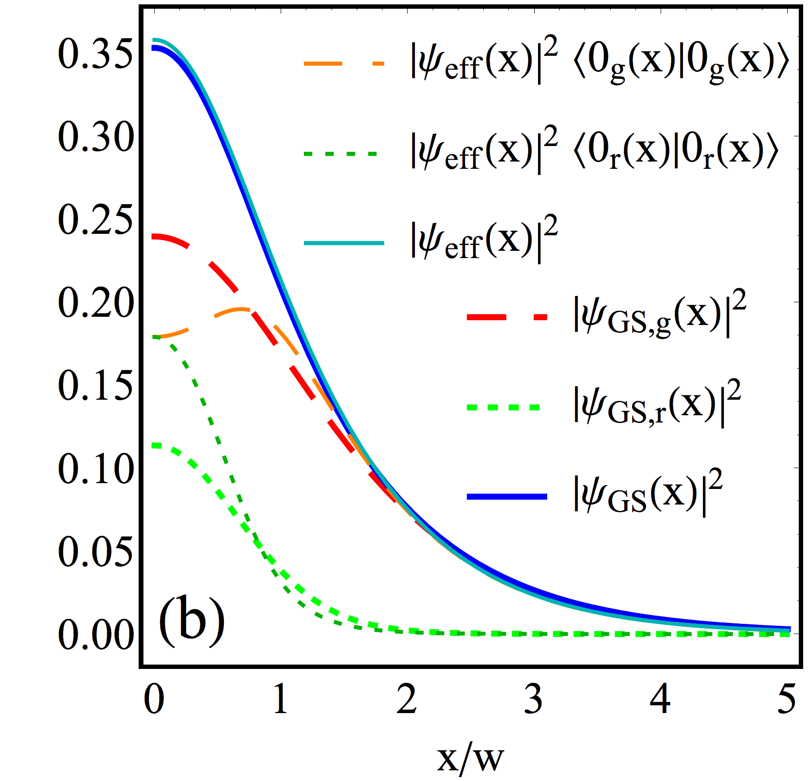
Figure 2: Analysis of the blue-detuned AC-Stark scheme [Fig. 1(b)]. (a) The light-shift $E_{0}(x)$, as well as the diagonal and off-diagonal couplings coming from the non-adiabatic potential $U$ in Eq. (14) parametrized by $\alpha$ and $\beta$. (b) Properties of the ground state obtained from the effective Hamiltonian and from the full Hamiltonian (see main text for details). Figures are shown in units of $w$ and $E_{w}$ making them applicable to all $s\gg 1$.

Note that the off-diagonal terms are significantly greater than the diagonal ones (i.e., $\alpha<|\beta|$), especially for $x\lesssim w$, as shown in Fig. 2(a). For $\Omega_{p}=E_{w}$, which leads to a single bound state, we obtain $\beta$ on the order of the energy $E_{0}(x)$. Note that our derivation works for arbitrary fractional probabilities $f_{r}=|{\psi_{r}(x)}/{\psi(x)}|$, whereas the method in Ref. Yavuz et al. (2009) works only for fractional probabilities $f_{r}\ll 1$, where $\psi_{r}=\innerproduct{r}{\psi}$ is the $r$-component of the ground-state wave function $\psi$.

In order to analyze the impact of $U$, we compare the ground-state of the effective Hamiltonian $H_{\rm\scriptscriptstyle eff}=E_{0}(x)-\frac{\partial_{x}^{2}}{2m}$ without $U$ with the exact solution of the full Hamiltonian given by Eqs. (1) and (8). Even though $|\bra{0}U\ket{+}|\sim E_{w}\sim\Omega_{p}$ is large and on the order of the energy difference $E_{+}-E_{0}\sim\Omega_{p}$, we see in Fig. 2(b) that the probability densities (and therefore the widths) of the ground states $\psi_{\rm\scriptscriptstyle eff}$ of $H_{\rm\scriptscriptstyle eff}$ and $\psi_{\rm\scriptscriptstyle GS}$ of the full Hamiltonian are nearly the same. However, from the comparison of components $\ket{g}$ and $\ket{r}$ of the ground state in Fig. 2(b), we see that the trapped atoms are not exactly in the eigenstate $\ket{0}$. This partially explains why the non-adiabatic corrections do not influence the width of the ground state: the components of the true ground state are smoother (spatial gradients are smaller) than than those of the ground state $\ket{0}$ of $H_{\rm\scriptscriptstyle al}$, which leads to weaker non-adiabatic corrections for the true ground state. In summary, even though the non-adiabatic potential $U$ can be on the order of $E_{w}$ for subwavelength traps, the width of the ground state is only very weakly influenced by $U$.

We now turn to the analysis of the trap lifetime. The leading contribution to losses comes from the admixture $P_{e}$ of the short-lived state $\ket{e}$. $P_{e}$ is determined by the characteristic coupling strength $\Omega_{c}(w)\approx\Omega_{0}/s$ within the trapped region and by the detuning $\Delta$ as $P_{e}\sim(\Omega_{0}/(\Delta s))^{2}\sim s^{6}(E_{\sigma}/\Omega_{0})^{2}$. In principle, the condition $\Delta>\Omega_{0}$ might give an upper limit on $s$, which, based on Eq. (11), for $\Omega_{p}=E_{w}$, is $s^{4}<\Omega_{0}/E_{\sigma}$. However, this is not a constraint for any of the results considered in this Letter.

Red-detuned AC-Stark scheme.—Finally, we analyze the third scheme, which was proposed in Ref. Yavuz et al. (2009). Our analysis, compared to the original one, takes into account non-adiabatic corrections and works for arbitrary fractional probabilities. This scheme differs from the blue-detuned AC-Stark scheme in that: first, the control Rabi frequency is $\Omega_{c}(x)=\Omega_{0}e^{-x^{2}/(2\sigma^{2})}$ which, for small $x$, is $\approx\Omega_{0}(1-x^{2}/(2\sigma^{2}))$; second, the detuning $\delta=\Omega^{2}_{0}/\Delta$ is chosen to exactly compensate for the AC-Stark shift at the center of the trap ; third, the detuning $\Delta$ now indicates the amount of red detuning. The resulting $E_{0}$ $w$, and $s$ are identical to those in the blue-detuned AC-Stark scheme, Eqs. (10) and (11). We find that, for $x\lesssim w$, the non-adiabatic corrections have nearly exactly the same form as in the blue-detuned AC-Stark scheme and differ only in the sign of the off-diagonal terms: $U=\left(\begin{array}[]{cc}\alpha&\beta\\ -\beta&\alpha\\ \end{array}\right).$

To derive the lifetime of this trap, we can set $\Omega_{c}(x)$ to $\Omega_{0}$ within the trapped region, which leads to $P_{e}\sim(\Omega_{0}^{2}/\Delta^{2})=(s^{2}\Omega_{p}/\Omega_{0})^{2}=s^{8}(E_{\sigma}/\Omega_{0})^{2}$. This expression is identical to the one in the EIT and blue-detuned AC-Stark schemes, except for the more favorable scaling with $s$ in our two schemes ($s^{6}$ vs. $s^{8}$), making them superior. The intuition behind the difference between the two schemes based on the AC-Stark shift is the following: in the red-detuned AC-Stark scheme, the atoms are trapped in the region of maximal scattering from state $\ket{e}$, whereas, in our blue-detuned AC-Stark scheme, atoms are trapped in the region of minimal scattering from state $\ket{e}$.

Atomic levels.—The level structure needed for the two AC-Stark schemes is most easily achieved with alkaline-earth atoms, in which $\ket{g}$, $\ket{r}$, and $\ket{e}$ are chosen to be the ground state ${}^{1}S_{0}$, the metastable state ${}^{3}P_{2}$, and the state ${}^{3}D_{2}$, respectively , see Fig. 3(a). The optical separation between the two long-lived states allows the decoupling of $\Omega_{c}$ from $\ket{g}$ to be a much better approximation  than what is possible in alkali atoms, where the size of $\Delta$ is limited by the fine structure splitting between the D1 and D2 lines Yavuz et al. (2009).

Turning now to the EIT scheme, the subwavelength trap depths achievable with the atomic levels used for barriers in Ref. Yang et al. (2018) are limited due to the off-resonant $\Omega_{c}$-induced coupling of $\ket{g}$ to $\ket{{}^{3}P_{1},F=3/2}$ , which is detuned by $\Delta_{\rm\scriptscriptstyle hfs}/2\pi=5.94$GHz from $\ket{{}^{3}P_{1},F=1/2}$. This coupling gives rise to a position-dependent light-shift of $\ket{g}$ and leads to an additional constraint $\Omega_{c}\ll\sqrt{\Delta_{\rm\scriptscriptstyle hfs}E_{w}}$ for trap realization. A solution [similar to the one used for the two AC-Stark schemes] is to protect our three-level system by an optical separation, as shown in Fig. 3(b)  .

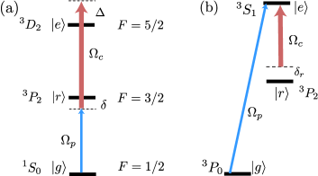
Figure 3: (a) Atomic levels for the two AC-Stark schemes. The decay rate from the metastable state ${}^{3}P_{2}$ is negligible ($\Gamma_{\rm\scriptscriptstyle 3P2}/2\pi=0.02$Hz). (b) Atomic levels for the EIT scheme. In all schemes, the main limitation comes from the admixture of levels outside the 3-level system.

Note that the atomic level configurations in Fig. 3 do not rely on optical polarization selection rules. Therefore, unlike the level configuration of Ref. Wang et al. (2018), such subwavelength traps can be extended into 3D.

Achievable trap parameters.—We showed above that, for fixed $\Omega_{0}$, the two schemes proposed in this Letter provide superior performance to the red-detuned AC-Stark scheme due to the $s^{6}$ vs. $s^{8}$ scaling of the losses. We now discuss what widths of the trapping potentials are achievable when we include fundamental limitations imposed on the magnitude of $\Omega_{0}$. We set the trapping time $T$ to be equal González-Tudela et al. (2015) to $10$ms, and consider ¹⁷¹Yb. Depending on the scheme and on $\sigma$ [equal to $\lambda/2\pi$ for the lattice, and to $3\mu m$ for the tweezer; denoted by subscripts _λ and _3μm, respectively], we find maximal $\Omega_{0}$ and $s$ such that the off-resonant position-dependent light-shifts are less than $0.1E_{w}$ and that $T\Gamma P_{e}\sim 1$:

$$\begin{array}[]{c|c|cc|c|cc}\text{setup}&\frac{\Omega_{0,\lambda}}{2\text{$\pi$GHz}}&\frac{w_{\lambda}}{\text{nm}}&s_{\lambda}&\frac{\Omega_{0,3\text{$\mu$m}}}{2\text{$\pi$GHz}}&\frac{w_{3\text{$\mu$m}}}{\text{nm}}&s_{3\mu m}\\ \hline\cr$EIT $&13&7.8&16.&2.6&39.&78.\\ $\text{blue-ac}$&4.1&8.8&36.&1.3&27.&111.\\ $\text{red-ac}$&1.2&29.&11.&0.28&130.&23.\end{array}$$ (19)

We see that the EIT and the blue-detuned AC-Stark schemes allow for greater $\Omega_{0}$, which translates into narrower traps. For comparison, alkali-atom-based EIT Wang et al. (2018) and red-detuned AC-Stark Yavuz et al. (2009) schemes are limited to $\Omega_{0,\lambda}/2\pi=400\text{MHz}$ (leading to $s=10$) and $\Omega_{0,\lambda}/2\pi=150\text{MHz}$ (leading to $s=1.7$), respectively.

Applications.—We now make a few remarks related to the applications pointed out in the introduction. Note that, if one’s goal is simply to use the expansion of a control field $\Omega_{c}(x)$ around its nodes to create traps with tight bound states with minimal scattering, then our EIT scheme has no advantages over a simple two-level blue-detuned trap. Indeed, in our case, up to an additive constant, the potential near a node is given by $V(x)\approx\delta_{r}\Omega_{c}(x)^{2}/\Omega_{p}^{2}$, while the population of the excited state is given by $P_{e}(x)\approx\delta_{r}^{2}\Omega_{c}^{2}(x)/\Omega_{p}^{4}$. On the other hand, if one uses the same field $\Omega_{c}(x)$ to create a simple two-level blue-detuned trap (with detuning $\Delta$), one obtains $V(x)\approx\Omega_{c}^{2}(x)/\Delta$ and $P_{e}(x)\approx\Omega_{c}^{2}(x)/\Delta^{2}$. In other words, our scheme is identical to the two-level scheme provided one replaces $\Delta$ with $\Omega_{p}^{2}/\delta_{r}$.

However, our goal is not only to create a tight bound state in a trap of subwavelength width $w$ but also to make the trapping potential nearly constant for $|x|>w$ so that we can make and possibly independently move several traps, or a full lattice of traps, with subwavelength separations. In that case, a simple two-level scheme will not work. Instead, one has to use one of the subwavelength schemes we discuss in this Letter.

In combination with stroboscopic techniques Nascimbene et al. (2015) or multi-level atomic schemes Łacki et al. (2016), our traps can lead to the creation of lattices with subwavelength periods, giving rise to large energy scales in Hubbard models Gross and Bloch (2017); Cazalilla et al. (2009); Gorshkov et al. (2010); Daley (2011); Cazalilla and Rey (2014) and in dipolar atomic Baier et al. (2016); Ferrier-Barbut et al. (2016); de Paz et al. (2013) and molecular Micheli et al. (2006); Baranov (2008); Pupillo et al. (2009); Carr et al. (2009); Gorshkov et al. (2011a, b); Yan et al. (2013); Covey et al. (2016); Moses et al. (2015) systems, with applications to quantum simulation and quantum computing. Movable subwavelength traps with subwavelength separation may also find applications in ultracold chemistry Dirk-Sören Lühmann et al. (2015); Ospelkaus et al. (2010); Liu et al. (2018).

I Supplemental material

In Sec. I.1, we discuss how to modify the EIT scheme to suppress non-adiabatic corrections. In Sec. I.2, we estimate losses to lower dressed states.

I.1 Modified EIT scheme

Here, we show how to suppress non-adiabatic corrections in the EIT scheme. The idea is that $\Omega_{c}(0)$ does not necessarily have to go to zero and that the gradient of $\Omega_{c}(x)$ around $x=w$ can be smaller than for linear $\Omega_{c}(x)\sim x\Omega_{0}/\sigma$. Non-adiabatic corrections can then be suppressed by using the following control field Yang et al. (2018): $\Omega_{c}(x)=\Omega_{0}(1+\nu-\cos(kx))$, which does not go to zero as deeply and as sharply as the linear $\Omega_{c}(x)$.

Expanding $\Omega_{c}(x)$ around a minimum for $\nu>0$, we find

$$\Omega_{c}(x)=\Omega_{p}(\eta+(x/w)^{2}),$$ (S1)

with $\eta=\nu\,\Omega_{0}/\Omega_{p}$ and $w=\frac{1}{k}\sqrt{2\Omega_{p}/\Omega_{0}}$, and which gives rise to

$$V_{\rm\scriptscriptstyle tot} = \frac{\delta_{r}}{\left(\eta+(x/w)^{2}\right)^{2}+1}\!+\!\frac{4E_{w}(x/w)^{2}}{\left((\eta+(x/w)^{2})^{2}+1\right)^{2}},$$

whose depth can be tuned to accommodate one or more bound states. By operating at $\eta>0$, we can use appropriate $|\delta_{r}|\sim E_{w}$ to engineer trapping potentials with negligible non-adiabatic potential $U$. Therefore, when it comes to losses, this modified EIT scheme allows us to gain up to a factor of $\sim 2$.

I.2 Landau-Zener estimates of losses to lower dressed states

Another source of losses is tunneling from the single bound state we consider to state $\ket{-}$. Note that, due to the conservation of energy, atoms in $\ket{-}$ will have large kinetic energy. Following Yi et al. (2008), the loss rate $\Gamma_{\rm\scriptscriptstyle LZ}$ can be estimated using a Landau-Zener like argument, which, in our setup, leads to

$$\Gamma_{\rm\scriptscriptstyle LZ}\sim E_{w}e^{-\nu\Delta_{0-}/E_{w}},$$ (S2)

where $\nu$ is a factor of order unity, and $\Delta_{0-}$ is the energy difference between two dressed states involved in the tunneling.

In the EIT scheme, we have $\Delta_{0-}\sim|E_{-}(0)|\sim\Omega_{p}$ because the tunneling occurs around $x\sim 0$ where the gap between $E_{D}$ and $E_{-}$ is smallest and where the atoms are trapped. This leads to the condition $1\ll\Omega_{p}/E_{w}=\Omega_{c}/(E_{\sigma}s^{3})$. Note that we obtained the same condition from the requirement $E_{w}\ll\Omega_{p}$, which enabled us to treat non-adiabatic potentials and light-shifts separately and perturbatively. We can further suppress tunneling losses by working at $\Delta\neq 0$.

In the blue-detuned AC-Stark scheme, $\Delta_{0-}\sim|E_{-}|\sim|\Delta|$, so this tunneling loss rate is strongly suppressed as $\exp[-|\Delta|/E_{w}]$.

In the red-detuned AC-Stark scheme, there is no state below the state of interest and therefore no tunneling.

References

- Gross and Bloch (2017) C. Gross and I. Bloch, Science 357, 995 (2017).
- Lewenstein et al. (2012) M. Lewenstein, A. Sanpera, and V. Ahufinger, Ultracold Atoms in Optical Lattices: Simulating quantum many-body systems ("Oxford University Press", 2012).
- González-Tudela et al. (2015) A. González-Tudela, C. L. Hung, D. E. Chang, J. I. Cirac, and H. J. Kimble, Nat. Photonics 9, 320 (2015).
- Mitsch et al. (2014) R. Mitsch, C. Sayrin, B. Albrecht, P. Schneeweiss, and A. Rauschenbeutel, Nat. Commun. 5, 5713 (2014).
- Thompson et al. (2013) J. D. Thompson, T. G. Tiecke, N. P. de Leon, J. Feist, A. V. Akimov, M. Gullans, A. S. Zibrov, V. Vuletić, and M. D. Lukin, Science 340, 1202 (2013).
- Chang et al. (2009) D. E. Chang, J. D. Thompson, H. Park, V. Vuletić, A. S. Zibrov, P. Zoller, and M. D. Lukin, Phys. Rev. Lett. 103, 123004 (2009).
- Gullans et al. (2012) M. Gullans, T. G. Tiecke, D. E. Chang, J. Feist, J. D. Thompson, J. I. Cirac, P. Zoller, and M. D. Lukin, Phys. Rev. Lett. 109, 235309 (2012).
- Romero-Isart et al. (2013) O. Romero-Isart, C. Navau, A. Sanchez, P. Zoller, and J. I. Cirac, Phys. Rev. Lett. 111, 145304 (2013).
- Agarwal and Kapale (2006) G. S. Agarwal and K. T. Kapale, J. Phys. B At. Mol. Opt. Phys. 39, 3437 (2006).
- Bajcsy et al. (2003) M. Bajcsy, A. S. Zibrov, and M. D. Lukin, Nature 426, 638 (2003).
- Dutton et al. (2001) Z. Dutton, M. Budde, C. Slowe, and L. V. Hau, 293, 663 (2001).
- Gorshkov et al. (2008) A. V. Gorshkov, L. Jiang, M. Greiner, P. Zoller, and M. D. Lukin, Phys. Rev. Lett. 100, 093005 (2008).
- Juzeliunas (2007) G. Juzeliunas, Lith. J. Phys. 47, 351 (2007).
- Miles et al. (2013) J. A. Miles, Z. J. Simmons, and D. D. Yavuz, Phys. Rev. X 3, 031014 (2013).
- Sahrai et al. (2005) M. Sahrai, H. Tajalli, K. T. Kapale, and M. S. Zubairy, Phys. Rev. A 72, 013820 (2005).
- Yavuz and Proite (2007) D. D. Yavuz and N. A. Proite, Phys. Rev. A 76, 041802(R) (2007).
- Subhankar et al. (2018) S. Subhankar, Y. Wang, S. L. Rolston, and J. V. Porto, arXiv:1807.02871v1 (2018).
- Mcdonald et al. (2018) M. Mcdonald, J. Trisnadi, K.-X. Yao, and C. Chin, arXiv:1807.02906v1 (2018).
- Yavuz et al. (2009) D. D. Yavuz, N. A. Proite, and J. T. Green, Phys. Rev. A 79, 055401 (2009).
- Łacki et al. (2016) M. Łacki, M. A. Baranov, H. Pichler, and P. Zoller, Phys. Rev. Lett. 117, 233001 (2016).
- Jendrzejewski et al. (2016) F. Jendrzejewski, S. Eckel, T. G. Tiecke, G. Juzeliunas, G. K. Campbell, L. Jiang, and A. V. Gorshkov, Phys. Rev. A 94, 063422 (2016).
- Wang et al. (2018) Y. Wang, S. Subhankar, P. Bienias, M. Łacki, T. C. Tsui, M. A. Baranov, A. V. Gorshkov, P. Zoller, J. V. Porto, and S. L. Rolston, Phys. Rev. Lett. 120, 083601 (2018).
- Yi et al. (2008) W. Yi, A. J. Daley, G. Pupillo, and P. Zoller, New J. Phys. 10, 073015 (2008).
- Lundblad et al. (2008) N. Lundblad, P. J. Lee, I. B. Spielman, B. L. Brown, W. D. Phillips, and J. V. Porto, Phys. Rev. Lett. 100, 150401 (2008).
- Perczel et al. (2017) J. Perczel, J. Borregaard, D. E. Chang, H. Pichler, S. F. Yelin, P. Zoller, and M. D. Lukin, Phys. Rev. Lett. 119, 023603 (2017).
- Grankin et al. (2018) A. Grankin, D. V. Vasilyev, P. O. Guimond, B. Vermersch, and P. Zoller, 1802.05592 (2018).
- Barredo et al. (2016) D. Barredo, S. De Leseleuc, V. Lienhard, T. Lahaye, and A. Browaeys, Science 354, 1021 (2016).
- Endres et al. (2016) M. Endres, H. Bernien, A. Keesling, H. Levine, E. R. Anschuetz, A. Krajenbrink, C. Senko, V. Vuletic, M. Greiner, and M. D. Lukin, Science 354, 1024 (2016).
- Dirk-Sören Lühmann et al. (2015) Dirk-Sören Lühmann, C. Weitenberg, and K. Sengstock, Phys. Rev. X 5, 031016 (2015).
- Ospelkaus et al. (2010) S. Ospelkaus, K. K. Ni, D. Wang, M. H. De Miranda, B. Neyenhuis, G. Quéméner, P. S. Julienne, J. L. Bohn, D. S. Jin, and J. Ye, Science 327, 853 (2010).
- Liu et al. (2018) L. R. Liu, J. D. Hood, Y. Yu, J. T. Zhang, N. R. Hutzler, T. Rosenband, and K. K. Ni, Science 903, 900 (2018).
- Kapale (2013) K. T. Kapale, in Prog. Opt., Progress in Optics, Vol. 58, edited by E. Wolf (Elsevier, 2013) pp. 199–250.
- Johnson et al. (1998) K. S. Johnson, J. H. Thywissen, N. H. Dekker, K. K. Berggren, A. P. Chu, R. Younkin, and M. Prentiss, Science 280, 1583 (1998).
- Thomas (1989) J. E. Thomas, Opt. Lett. 14, 1186 (1989).
- Stokes et al. (1991) K. D. Stokes, C. Schnurr, R. Gardner, M. Marable, G. Welch, and J. Thomas, Phys. Rev. Lett 67, 1997 (1991).
- Schrader et al. (2004) D. Schrader, I. Dotsenko, M. Khudaverdyan, Y. Miroshnychenko, A. Rauschenbeutel, and D. Meschede, Phys. Rev. Lett. 93, 150501 (2004).
- Gardner et al. (1993) J. R. Gardner, M. L. Marable, G. R. Welch, and J. E. Thomas, Phys. Rev. Lett. 70, 3404 (1993).
- Zhang et al. (2006) C. Zhang, S. L. Rolston, and S. Das Sarma, Phys. Rev. A 74, 042316 (2006).
- Lee et al. (2007) P. J. Lee, M. Anderlini, B. L. Brown, J. Sebby-Strabley, W. D. Phillips, and J. V. Porto, Phys. Rev. Lett. 99, 020402 (2007).
- Kapale and Agarwal (2010) K. T. Kapale and G. S. Agarwal, Opt. Lett. 35, 2792 (2010).
- Le Kien et al. (1997) F. Le Kien, G. Rempe, W. P. Schleich, and M. S. Zubairy, Phys. Rev. A 56, 2972 (1997).
- Qamar et al. (2000) S. Qamar, S. Y. Zhu, and M. S. Zubairy, Phys. Rev. A 61, 063806 (2000).
- Paspalakis and Knight (2001) E. Paspalakis and P. L. Knight, Phys. Rev. A 63, 065802 (2001).
- Hell (2007) S. W. Hell, Science 316, 1153 (2007).
- Li et al. (2008) H. Li, V. A. Sautenkov, M. M. Kash, A. V. Sokolov, G. R. Welch, Y. V. Rostovtsev, M. S. Zubairy, and M. O. Scully, Phys. Rev. A 78, 013803 (2008).
- Mompart et al. (2009) J. Mompart, V. Ahufinger, and G. Birkl, Phys. Rev. A 79, 053638 (2009).
- Sun et al. (2011) Q. Sun, M. Al-Amri, M. O. Scully, and M. S. Zubairy, Phys. Rev. A 83, 063818 (2011).
- Proite et al. (2011) N. A. Proite, Z. J. Simmons, and D. D. Yavuz, Phys. Rev. A 83, 041803(R) (2011).
- Qi et al. (2012) Y. Qi, F. Zhou, T. Huang, Y. Niu, and S. Gong, J. Mod. Opt. 59, 1092 (2012).
- Viscor et al. (2012) D. Viscor, J. L. Rubio, G. Birkl, J. Mompart, and V. Ahufinger, Phys. Rev. A 86, 063409 (2012).
- Yavuz and Simmons (2012) D. D. Yavuz and Z. J. Simmons, Phys. Rev. A 86, 013817 (2012).
- Rubio et al. (2013) J. L. Rubio, D. Viscor, and V. Ahufinger, Opt. Express 21, 022139 (2013).
- Note (1) Such an intensity profile can be approximately implemented by using existing techniques such as intensity masks Eckel et al. (2014), Hermite-Gaussian laser modes, or holographic techniques Gaunt et al. (2013).
- (54) “See Supplement for details.” .
- Note (2) Depending on the desired parameters of the trap, choosing a slightly larger detuning can sometimes slightly improve the scheme by achieving the optimal trade off between non-adiabaticity and scattering. However, the improvement is insignificant, so we chose to focus on to simplify the presentation.
- Note (3) The transition has greater matrix element Porsev and Derevianko (2004) than transition , which makes it possible to work with greater .
- Note (4) The main limitation comes from the off-resonant coupling of by the field to , , and .
- Yang et al. (2018) D. Yang, C. Laflamme, D. V. Vasilyev, M. A. Baranov, and P. Zoller, Phys. Rev. Lett. 120, 133601 (2018).
- Note (5) More precisely, couples = to .
- Note (6) The main limitation comes from the coupling of to the , , and manifolds.
- Nascimbene et al. (2015) S. Nascimbene, N. Goldman, N. R. Cooper, and J. Dalibard, Phys. Rev. Lett. 115, 140401 (2015).
- Cazalilla et al. (2009) M. A. Cazalilla, A. F. Ho, and M. Ueda, New J. Phys. 11, 103033 (2009).
- Gorshkov et al. (2010) A. V. Gorshkov, M. Hermele, V. Gurarie, C. Xu, P. S. Julienne, J. Ye, P. Zoller, E. Demler, M. D. Lukin, and A. M. Rey, Nat. Phys. 6, 289 (2010).
- Daley (2011) A. J. Daley, Quantum Inf. Process. 10, 865 (2011).
- Cazalilla and Rey (2014) M. A. Cazalilla and A. M. Rey, Reports Prog. Phys. 77, 124401 (2014).
- Baier et al. (2016) S. Baier, M. J. Mark, D. Petter, K. Aikawa, L. Chomaz, Z. Cai, M. Baranov, P. Zoller, and F. Ferlaino, Science 352, 201 (2016).
- Ferrier-Barbut et al. (2016) I. Ferrier-Barbut, H. Kadau, M. Schmitt, M. Wenzel, and T. Pfau, Phys. Rev. Lett. 116, 215301 (2016).
- de Paz et al. (2013) A. de Paz, A. Sharma, A. Chotia, E. Maréchal, J. H. Huckans, P. Pedri, L. Santos, O. Gorceix, L. Vernac, and B. Laburthe-Tolra, Phys. Rev. Lett. 111, 185305 (2013).
- Micheli et al. (2006) A. Micheli, G. K. Brennen, and P. Zoller, Nat. Phys. 2, 341 (2006).
- Baranov (2008) M. A. Baranov, Phys. Rep. 464, 71 (2008).
- Pupillo et al. (2009) G. Pupillo, A. Micheli, H. P. Büchler, and P. Zoller, Cold Mol. Theory, Exp. Appl. 322, 421 (2009).
- Carr et al. (2009) L. D. Carr, D. DeMille, R. V. Krems, and J. Ye, New J. Phys. 11, 055049 (2009).
- Gorshkov et al. (2011a) A. V. Gorshkov, S. R. Manmana, G. Chen, J. Ye, E. Demler, M. D. Lukin, and A. M. Rey, Phys. Rev. Lett. 107, 115301 (2011a).
- Gorshkov et al. (2011b) A. V. Gorshkov, S. R. Manmana, G. Chen, E. Demler, M. D. Lukin, and A. M. Rey, Phys. Rev. A 84, 033619 (2011b).
- Yan et al. (2013) B. Yan, S. A. Moses, B. Gadway, J. P. Covey, K. R. Hazzard, A. M. Rey, D. S. Jin, and J. Ye, Nature 501, 521 (2013).
- Covey et al. (2016) J. P. Covey, S. A. Moses, M. Gärttner, A. Safavi-Naini, M. T. Miecnikowski, Z. Fu, J. Schachenmayer, P. S. Julienne, A. M. Rey, D. S. Jin, and J. Ye, Nat. Commun. 7, 24 (2016).
- Moses et al. (2015) S. A. Moses, J. P. Covey, M. T. Miecnikowski, B. Yan, B. Gadway, J. Ye, and D. S. Jin, Science 350, 659 (2015).
- Eckel et al. (2014) S. Eckel, J. G. Lee, F. Jendrzejewski, N. Murray, C. W. Clark, C. J. Lobb, W. D. Phillips, M. Edwards, and G. K. Campbell, Nature 506, 200 (2014).
- Gaunt et al. (2013) A. L. Gaunt, T. F. Schmidutz, I. Gotlibovych, R. P. Smith, and Z. Hadzibabic, Phys. Rev. Lett. 110, 200406 (2013).
- Porsev and Derevianko (2004) S. G. Porsev and A. Derevianko, Phys. Rev. A 69, 042506 (2004).