Student Log-Data from a Randomized Evaluation of Educational Technology: A Causal Case Study

1 Introduction

From 2007 through 2010, the RAND corporation conducted one of the first effectiveness trials awarded through competitive grant programs sponsored by the US Department of Education’s Institute of Education Sciences. The randomized controlled trial (RCT) was designed to estimate the effect of school-wide adoption of the Cognitive Tutor Algebra I (CTA1) curriculum, whose centerpiece is a computerized “tutor” that uses cognitive science principles to teach Algebra I (Anderson et al., 1985). The study (Pane et al., 2014) found no effects in its first year, but in the second year of implementation students in high schools randomized to the CTA1 condition outperformed the control group on the posttest by a fifth of a standard deviation. As educational technology (EdTech) booms, so do RCTs in the mold of the RAND CTA1 study. A recent systematic review (Escueta et al., 2017) cites 29 published reports of RCTs of “computer assisted learning” programs, all but one of which was published since 2001. We are aware of numerous other such RCTs planned or ongoing.

RCTs are invaluable tools for estimating these programs’ efficacy. However, the interventions they study are highly multifaceted and complex. Each classroom, and each student within those classrooms, may use an EdTech application in a different way; presumably, the application’s efficacy depends on these usage decisions. Similarly, EdTech applications often include a number of optional features—to what extent do each of these drive the program’s effectiveness? The data collected during typical education RCTs—data on treatment assignments, outcomes, a standard set of demographics, and possibly a pretest—offer limited options for studying treatment effect heterogeneity, and offer no information on how the intervention was implemented.

However, with little extra effort, researchers studying EdTech can gather rich implementation data over the course of an RCT. For instance, the software administrators running the CTA1 RCT gathered computer log data for students in the treatment group. They assembled a dataset that recorded which problems each student worked, along with timestamps, the numbers of hints requested, and the number of errors committed for each problem. Analogous log data is (or may be) collected from other EdTech RCTs. As one example, RAND recently completed an efficacy study of a different algebra tutoring system, ALEKS, and gathered student log data in order to study implementation.

Analysis of log data from EdTech RCTs could, in principle, lead to insights on the relationship between implementation and effectiveness. Using log data, researchers could investigate how the product was actually implemented, as well as what aspects of implementation correlate with higher (or lower) treatment effects, or which features of the program drive its effects. For instance, Sales et al. (2016); Sales and Pane (2019a, 2020) investigated aspects of mastery learning with CTA1. An ongoing research project uses the ALEKS log data to study its instructional material: when students begin working on a particular topic in ALEKS, the system first presents instructional material, followed by problem solving activities, and then, if students are unsuccessful at solving the problems, more instructional material. Some students diligently read the initial instructional material while others skip it and dive directly into problem solving. Is skipping the material a productive strategy for students in terms of learning algebra, or should ALEKS be redesigned to prevent such skipping?

Answering questions like these calls for new statistical tools, which must simultaneously surmount three challenges: first, implementation is not typically randomized, so the relationship between log data and outcomes is likely confounded. Second, log data is only gathered from students assigned to use the intervention, and not from the control group. Third, log datasets have a complex structure—often a large number of granular observations of several types gathered over the course of each student’s engagement with the program.

This paper will use log data from the CTA1 study—specifically, data on students’ use of hints within the software—to illustrate three approaches to these challenges. We will attempt to answer two related questions: first, what is the role of the availability of hints in driving the overall CTA1 treatment effect? Second, can requesting hints more often lead to a larger treatment effect? The first approach we consider discards the control group, and analyzes hint-requesting in the treatment group as an observational study, using a matching design (c.f. Rosenbaum, 2002). The second approach applies the framework of causal mediation analysis (VanderWeele, 2015; Hong, 2015; Imai et al., 2011) to estimate the role of hint-requesting in the overall CTA1 treatment effect. However, since students in the control group were unable to request hints, not all mediational estimands are identified, and estimation methods must be modified. Finally, we conduct a principal stratification analysis (Frangakis and Rubin, 2002) to learn if students requesting hints at different rates experienced different treatment effects.

Our intention is to develop, demonstrate, and contrast these three approaches to modeling log data. A rich, and often polemic, literature surrounds principal stratification and mediation analysis (e.g. Rubin, 2004; VanderWeele, 2011; Pearl, 2011; Mealli and Mattei, 2012; VanderWeele, 2012). VanderWeele (2008), Jo (2008) and others have given conditions under which certain principal stratification and mediational estimands coincide. Our contribution will build on this literature in two ways: first, by providing a detailed demonstration and comparison of matching, mediation analysis, and principal stratification on the same dataset, and second by focusing on the applicability of these three methods in the specific context of studying implementation data from an randomized experiment studying educational technology.

The following section will provide background for the case-study, describing the CTA1 curriculum, the RAND study, and our focus on hints. The next three sections will present the observational study, causal mediation, and principal stratification, respectively. As it turns out, these analyses appear to give contradictory results—the observational study and mediation analysis estimate a negative effect of requesting hints, while the principal stratification analysis finds that students who requested more hints may have experienced larger overall treatment effects. Section 6 will contrast these findings (including a possible reconciliation), compare the three methods generally, and discuss how they may be applied to data from other educational technology RCTs. Section 7 will conclude.

The R and Stan code used to for all of the analyses in the paper can be found in a github repository, https://github.com/adamSales/logDataCaseStudy.

2 Case Study: The Role of Hints in the Cognitive Tutor Effect

2.1 The Cognitive Tutor

CTA1 is one of a series of complete mathematics curricula developed by Carnegie Learning, Inc., which include both textbook materials and an automated computer-based Cognitive Tutor (Anderson et al., 1995; Pane et al., 2014).

The computerized tutor was originally built to test the ACT and ACT-R theories of cognition (Anderson, 2013). These are elaborate theories that describe, among other things, the necessary components of cognitive skills in, say, mathematics or computer programming, and the process of acquiring those skills. The Algebra I tutor guides students through a sequence of Algebra I problems nested in sections within units, and organized by the specific sets of skills they require. Students move through the curriculum as the tutor’s internal learning model determines that they have mastered the requisite skills.

2.2 The Role of Hints

Students using the Cognitive Tutor Algebra software work algebra problems on a computer. Each problem in the software is associated with a set of skills that the student must master in order to solve the problem. The software also specifies a “solution path” for each problem—a sequence of actions (such as “multiply both sides of the equation by 3”) students must take in order to solve the problem. If there is more than one way to solve a problem, the software specifies multiple correct solution paths students may follow. As soon as a student errs in working through a problem—that is, departs from one of the solution paths—the software shows the student an error message. This feedback is tailored to the specific mistake, and designed to guide the student back to a correct solution path. Similarly, when a student gets stuck, and is unable to determine the next step in solving the problem, he or she can ask for a hint. Like the error feedback, these hints are tailored to the specific algebra skills corresponding to the next step on the solution path. Thus, hints and error feedback are crucial aspects of the tutor’s pedagogy.

There are good reasons to believe that the availability of hints—help on demand—may increase student learning, but there is also reason to be skeptical (See Aleven et al., 2016, for an overview of the theory). First of all, as, e.g., Anderson et al. (1995) points out, “if students never receive help of any sort, they are in danger of becoming permanently stuck on some problem” (p. 190). That is, hints give students who are stuck a way to continue working. Hints may also boost learning by “helping students identify relevant features in problems” (Aleven et al., 2016, p. 6), that is, point students towards aspects of the problem that are “most important for the goals of learning” (Koedinger et al., 2012, p. 782). Hints can help improve students’ self-awareness and problem-solving strategy, such as by clarifying which skills they have and have not mastered.

Most problems are associated with several hints, arranged in a sequence so that a student who remains stuck after one hint may request another. The last hint in the sequence will show a complete solution to the problem—essentially showing students a worked example, which can be an effective tool for learning (e.g. Sweller and Cooper, 1985).

On the other hand, all of these theoretical mechanisms rely on students to play their part. In order for hints to be instructive, students need to reflect on their content in productive ways. This suggests that hints may be helpful for some students but not for others. In the same vein, hints need to be well-designed in order to be effective (McKendree, 1990), so some hints may be more helpful than others.

Hints may even be harmful: as Koedinger and Aleven (2007) put it (p. 241), “many lines of research and theory suggest the importance of …withholding information from students so that they can exercise, test, or reason toward new knowledge on their own.” Paas and Van Merriënboer (1994) interpret this dilemma in terms of balancing “cognitive load,” that is, optimally allocating a student’s attention to the most relevant aspects of a problem.

The empirical literature on the value of hints in intelligent tutors is mixed (see Goldin et al., 2012, for a summary). Anderson et al. (1995) compared the performance of students randomly assigned to different versions of the Cognitive Tutor with different feedback structures, and found that students who were able to request hints finished the lesson faster than those who were not, but could not detect an effect on learning. Singh et al. (2011) used a similar design, comparing two versions of the ASSISTments intelligent tutor, one in which hints and immediate error messages were available, and one which did not provide feedback. Students in the feedback condition showed larger gains on a posttest, though it is unclear whether these gains were due to hints or error feedback. Beck et al. (2008) and Goldin et al. (2012), did not randomize hint availability, but instead used statistical models to control for observed confounding. Both papers used students’ subsequent performance within the tutor to estimate hint effects. Beck et al. (2008) found conflicting results using different analytical methods to control for confounding. Goldin et al. (2012) investigated two sources of heterogeneity in the effect of a hint request: by student and by the “level” of the hint (the first, second, or final hint available for a given problem). They found that the effect of asking for a hint varies between students, but on average it is negative for the first two hints requested on a problem, but positive for the final hint.

2.3 Measuring Hint Usage in the CTA1 Data

Since the purpose of the CTA1 study was to estimate the overall effect of the CTA1 curriculum—including the associated textbook and recommended classroom practices—access to the full CTA1 curriculum was randomized, rather than any specific aspect of usage. Effectiveness was measured with a standardized posttest covering a broad range of Algebra I skills. In this regard, the CTA1 study is similar to other large-scale evaluations of educational technology which do not randomize usage but do include a posttest.

The CTA1 study was of a much longer duration than any of the studies of hint effects we are aware of: students had access to the tutor for an entire school year before the posttest. This factor allows for much more data for each student than shorter studies, as well as more variability in the types of problems and contexts in which students may request hints.

In order to align with our research focus, we narrow the type of hint data we model. Since our posttest measured Algebra I skills, we only considered worked problems from the Algebra I curriculum. Next, although Goldin et al. (2012) demonstrated the importance of hint level, our focus is on the overall average effect of requesting any hints; therefore, the variable measuring a student’s hint request on a problem was set to one if the student requested any hints on that problem, and zero otherwise.

Lastly, any observational study of hint usage must contend with the fact that students are unlikely to request hints on problems that they already know how to solve. Hence, any measure of hint usage is necessarily also a measure of student ability—students who know more algebra will almost certainly request fewer hints. This leads to two related problems: first, student ability confounds any statistical relationship between hint request frequency and posttest scores. Secondly, a student’s decision to request a hint implies both that she found the problem at least somewhat difficult, and that, in this case, she responded to that difficulty by requesting a hint. Our interest is in the second implication, not the first. Conversely, the significance of a student’s decision to forgo a hint depends in part on how challenging he or she finds the problem. Hint request frequency combines students’ hint requests (or non-requests) from both problems they find challenging and trivial, so is a poor measure of students’ disposition to use the hint feature.

Ideally, we would solve this problem by only including data on problem-student pairs in which the problem was challenging to the student. Of course, no direct measure of problem challenge is available. Instead, we considered a problem to be challenging if the student either requested a hint or made an error on that problem. Then, let

$$\bar{h}_{i}=\frac{\text{\# problems on which }i\text{ requested a hint}}{\text{\# problems on which }i\text{ either requested a hint or made an error}}$$

measure hint frequency.

This measure is inversely related to the ratio of the percentage (of all problems) a student makes an error without having requested a hint, to the percentage of problems a student requests a hint. Making an error on a problem without having requested a hint reflects a hesitance to request a hint when one might have been warranted (or a careless mistake). $\bar{h}$ ignores the class of challenging problems on which students are challenged and figure the answer out (or guess correctly) without requesting a hint. This class of problems is inherently interesting to our question; however, it is unidentified.

2.3.1 Dichotomizing Hint Usage

The observational study and mediation analysis below require a dichotomous measurement of hint usage: is a student a high or low hint user? To this end, we dichotomize $\bar{h}$ by comparing it to a cutoff value, so that $H_{i}=\mathbf{1}_{\left[{\bar{h}_{i}>c}\right]}$, where $\mathbf{1}_{\left[{x}\right]}=1$ if $x$ is true and 0 otherwise.

To choose $c$, we first fit a modified Rasch mixture model (Rasch, 1993) to hint request data. Specifically, we modeled the probability of at least one hint request in each problem $p$, worked by student $i$, in which $i$ requested a hint and/or committed an error, as

$$Pr(h_{ip})=logit^{-1}(\eta_{i}+\delta_{s[p]})$$ (1)

where $h_{ip}$ is the event that student $i$ requests at least one hint on problem $p$, $\eta_{i}$ is a student parameter, $\delta_{s[p]}$ is a section-level parameter for $s[p]$, the section that problem $p$ was drawn from, and $logit^{-1}(x)=\{1+exp(-x)\}^{-1}$ is the inverse logit function.

Typically, the student parameter $\eta_{i}$ measures student ability; here, instead, it measures a student’s proclivity to request a hint. The typical Rasch model includes a problem-level “difficulty” parameter; here, it would measure the likelihood an individual problem elicits a hint request. That parameter is important in our context because the specific problems a student works on may influence his or her hint requests. For instance, two students with the same underlying proclivity to request hints $\eta$ may actually differ in their observed hint requests, because one worked on harder problems than the other. However, in our dataset many problems were worked by very few students, so problem-level parameters would be hard to estimate. Instead, we included the section-level parameter $\delta_{s[p]}$, which measures the extent to which students tend to request hints on problems in section $s$. Ignoring the differences between problems within a section could allow for wider variance in the average problem difficulty each student experiences than is captured by the section level parameters $\delta_{s[p]}$. That could, in turn, induce a difference in hint requests between two students with similar $\eta$ or vice-versa, and lead to bias in our estimate of $\eta$. Since the Cognitive Tutor selects problems for students based on estimates of their current skill mastery (Fancsali et al., 2020), this possibility is not out of the question.

With even more granular data, (1) could be further elaborated, avoiding this assumption. In the Cognitive Tutor, problems often have multiple parts, and each part offers its own hints. Researchers in possession of data on each part of each worked problem could specify a model at the part-level, instead of at the problem-level like (1). Perhaps an even better option (suggested by an anonymous reviewer) would incorporate data on the specific skills required to solve each problem. While sections of the tutor differ from each other in the skills they teach, not every problem in each section includes the same set of skills; different problems requiring the same skill set will be similar in difficulty (Goldin et al., 2012; Pavlik Jr et al., 2009, see, e.g.).

In order to dichotomize hint request behavior, we modeled student effects $\eta$ as

$$\eta\sim p_{0}\mathcal{N}(\mu_{0},\sigma_{0})+(1-p_{0})\mathcal{N}(\mu_{1},\sigma_{1})$$ (2)

and constrained $\mu_{0}<\mu_{1}$. This mixture model clusters students into two categories: high hint users have $\eta$ drawn from a normal distribution with mean $\mu_{1}$ and standard deviation $\sigma_{1}$, and low hint users have $\eta$ drawn from a normal distribution with mean $\mu_{0}$ and standard deviation $\sigma_{0}$.

Our main parameter of interest here is $p_{0}$, the proportion of students who are low hint users. We estimated $p_{0}\approx$0.7, classifying 30% of students as high hint users, so we chose $c$ as the 70th percentile of $\bar{h}$, approximately 0.6. This definition agreed with the model’s classification (based on $\eta$ as opposed to $\bar{h}$) in approximately 93% of cases.

The Rasch model for hint usage (1), but not the mixture model (2) will play an important role in the principal stratification analysis of Section 5.

2.4 Data

(Pane et al., 2014) estimated effects separately in middle schools and high schools in each year of implementation; the only statistically significant treatment effect was in the high school sample in the second year. Since our goal was to better understand the CTA1 treatment effect, we focused our analysis on data from high school students in the second year of the CTA1 trial, for whom the treatment effect was most evident.

We merged data from two sources: computerized log data gathered by Carnegie Learning, and covariate, treatment and outcome data gathered by RAND.

The log data lists the problem name, section, and unit of each problem, the numbers of hints requested and errors committed, and time-stamps. Log data were missing for some students, either because the log files were not retrievable, or because of an imperfect ability to link log data to other student records. Further, log data for sections that were not part of the standard CTA1 Algebra I curriculum and sections worked by fewer than 100 students were omitted from the dataset.

To construct our analysis dataset, we first dropped treatment schools with log data missing for 90% or more students. Prior to randomization, schools were stratified into pairs or triples based on baseline covariates, and randomized between treatment and control condition within those randomization blocks. When we dropped a treatment school from our analysis, we also dropped the control schools in its randomization block. Of the remaining 2,390 students, 88% (2,108) had log data. Then, for the sake of simplicity, the treatment students without log data were dropped from the study.

All told, the analyses presented here were all based on 2,108 students assigned to the CTA1 condition; the estimation of direct effects in Section 4 and the principal stratification also relied on the 2,918 students assigned to control. Together, the 5,026 students were nested within 116 teachers, in 43 schools across five states.

Table 1 describes the covariates we used, including missingness information, control and treatment means, and standardized differences (c.f. Kalton, 1968) from the final analysis sample. We singly-imputed missing values with the Random Forest routine implemented by the missForest package in R (Stekhoven and Buehlmann, 2012; R Core Team, 2016), which estimated “out of box” imputation error rates as part of the random forest regression, also shown in Table 1.

	% Miss.	Imp. Err.	Levels	BaU	CTA1	Std. Diff.
Grade	3%	0.01	9th	91%	90%	-0.04
			$>$9th	9%	10%	0.04
ELL	4%	0.01	No	95%	96%	0.09
			Yes	5%	4%	-0.09
FRL	29%	0.29	No	26%	27%	0.02
			Yes	74%	73%	-0.02
Ethnicity	6%	0.23	White/Asian	47%	52%	0.16
			Black/Multi	32%	26%	-0.14
			Hispanic/Nat.Am.	21%	22%	-0.03
Sex	5%	0.35	Female	51%	49%	-0.04
			Male	49%	51%	0.04
Sp. Ed.	1%	0.11	Typical	87%	86%	-0.00
			Sp. Ed.	8%	8%	-0.02
			Gifted	5%	6%	0.03
Pretest	16%	0.20		-0.33	-0.36	-0.05
			Overall Covariate Balance: p=0.55

Table 1: Missingness information, control (“BaU” or “Business as Usual”) and treatment (“CTA1”) means, and balance for the covariates included in this study, from the high school year two stratum of CTA1 Effectiveness experiment. Imputation error is percent falsely classified for categorical variables (Race/Ethnicity, Sex, and Special Education) and standardized root mean squared error for Pretest, which is continuous. Analysis done in R via RItools (Bowers et al., 2017).

3 An Observational Study Within an Experiment

How does requesting hints within CTA1 affect learning? More precisely, would low hint users have achieved higher posttest scores had they requested hints more often? Would high hint users have achieved higher posttest scores had the requested hints less often?

This section will illustrate an observational study to answer these questions. Generally speaking, the observational study approach discards the control group entirely and uses statistical confounder control (in our case, propensity score matching) to estimate causal effects of a usage parameter on posttest scores. Implementing the method requires data from members of the treatment group: usage (in our case, $H$), posttest scores or another outcome of interest, and a set of baseline covariates to control for confounding. Since the control group is not used, identification does not depend on randomization—in fact, this same approach could be (and is) used with non-experimental data. However, outside of a planned experiment, posttest scores may not be available. Our usage variable $H$ is binary, which is necessary for classical propensity score matching; alternative methods are available for usage variable that are continuous (e.g. Hirano and Imbens, 2004), ordered (e.g. Leon and Hedeker, 2005), categorical (e.g. Lopez et al., 2017) or other types. Like all observational studies, it depends on the strong, untestable assumption of no unmeasured confounding.

The approach we take here, following Rosenbaum (2002), Hansen (2011), and Ho et al. (2007), has three broad steps. In the first, we construct a “match,” identifying groups of students, some of whom have $H=0$ and others with $H=1$, but who are otherwise comparable. The hope is that the distribution of $H$ conditional on this match resembles what might have been seen if (counterfactually) $H$ had been randomized within matched groups. Thus we evaluate the success of the match by checking if matched students have similar baseline covariate distributions; if necessary, we may revise match. In the second step, we estimate the average effect of $H$ on posttest scores, by comparing posttest scores between matched students with $H=1$ and $H=0$. In the third and final step, we account for the possibility of unmeasured confounding in a sensitivity analysis.

The next subsection will give more formal background on propensity score matching, including notation and identification assumptions. Following subsections will illustrate each of the three steps of propensity score matching.

3.1 Observational Study: Background

Let $Y_{i}$ represent subject $i$’s posttest score, and let $Z_{i}$ represent $i$’s treatment status (i.e. the CTA1 or control group). Following Neyman (1923) and Rubin (1978), let $Y_{i}(Z=1)$ be the posttest score student $i$ would achieve were $i$ (perhaps counterfactually) assigned to the treatment condition, and $Y_{i}(Z=0)$ the score were $i$ assigned to control. Then the CTA1 treatment effect for student $i$ is $Y_{i}(Z=1)-Y_{i}(Z=0)$. For students in the treatment group, define potential outcomes $Y_{i}(Z=1,H=1)$ and $Y_{i}(Z=1,H=0)$, or $Y_{i}(H=1)$ and $Y_{i}(H=0)$ for short, corresponding to $i$’s posttest score were $H_{i}=1$ or 0, respectively. Then the effect of $H$ on $Y$ for student $i$ is $Y_{i}(H=1)-Y_{i}(H=0)$. This structure implicitly assumes “non-interference,” that one student’s treatment assignment $Z$ or hint proclivity $H$ does not affect another student’s posttest scores.

Individual treatment effects are (typically) unidentified, since only one of the relevant potential outcomes is ever observed for each subject. For instance, $Y(H=1)$ is unobserved for members of the treatment group with $H=0$. If $Pr(H_{i}=1)$ were known for each $i$, and bounded away from 1 and 0, (as would be the case if $H$ were randomized) then the average treatment effect (ATE) of $H$ on $Y$, $\mathbb{E}[Y(H=1)]-\mathbb{E}[Y(H=0)]$, could be estimated without bias or further assumptions. Of course, the distribution of $H_{i}$ is unknown, and is presumably a function of $i$’s individual characteristics (which, as we shall see, differed at baseline between those students with $H=1$ and those with $H=0$).

Let $\bm{x}_{i}$ represent a vector of baseline covariates for subject $i$. In our study of hints, $\bm{x}$ includes indicators for state, school, and classroom, and the variables described in Table 1. Then we assume (c.f. Rosenbaum and Rubin, 1983):

• $$\{Y(H=1),Y(H=0)\}\mathchoice{\mathrel{\hbox to0.0pt{$\displaystyle\perp$\hss}\mkern 2.0mu{\displaystyle\perp}}}{\mathrel{\hbox to0.0pt{$\textstyle\perp$\hss}\mkern 2.0mu{\textstyle\perp}}}{\mathrel{\hbox to0.0pt{$\scriptstyle\perp$\hss}\mkern 2.0mu{\scriptstyle\perp}}}{\mathrel{\hbox to0.0pt{$\scriptscriptstyle\perp$\hss}\mkern 2.0mu{\scriptscriptstyle\perp}}}H|\bm{x}$$

that conditional on $\bm{x}$, potential outcomes $Y(H=1)$ and $Y(H=0)$ are independent of realized $H$. Under strong ignorability, one may compare subjects with identical covariates $\bm{x}$ to estimate causal effects.

Unfortunately, this sort of exact matching is impossible in our finite sample. Instead, we estimated “propensity scores” (Rosenbaum and Rubin, 1983):

$$\pi_{i}=Pr(H_{i}=1|\bm{x})$$

the probability of a treatment-group subject requesting frequent hints, conditional on his or her covariate vector $\bm{x}$. Rosenbaum and Rubin (1983) shows that conditioning on $\pi$ is equivalent to conditioning on $\bm{x}$. We estimated $\pi$ using a multilevel logistic regression, using the lme4 package in R (Bates et al., 2015). The propensity score model was:

$$\pi_{i}=logit^{-1}(\alpha+\bm{\tilde{x}}\bm{\beta}+\epsilon^{state}+\epsilon^{school}+\epsilon^{class})$$

where $\bm{\tilde{x}}$ is a vector of covariates including the variables in Table 1, missingness indicators for grade, race, sex, and economic disadvantage, and a natural spline with five degrees of freedom for pretest. State, school, and class were each included using normally distributed random intercepts, $\epsilon^{state}$, $\epsilon^{school}$, and $\epsilon^{class}$.

3.2 Constructing and Evaluating a Match

We constructed an optimal full matching design (Hansen, 2004) to condition on estimated propensity scores $\hat{\pi}$ using the optmatch package in R (Hansen and Klopfer, 2006). We matched $H=0$ subjects to $H=1$ subjects in such a way as to minimize the overall distance between subjects in matched sets in the logit-transformed propensity scores, $logit(\hat{\pi})$. We constrained the match so that students could only be matched within schools, since schools determine a number of factors that in turn may impact posttest scores, including baseline student characteristics, pedagogical styles, and CTA1 usage patterns (see Israni et al., 2018). Each matched set was allowed to contain any positive number of $H=1$ and any positive number of $H=0$ subjects, resulting in matches of variable size and composition. For instance, one matched set included 44 $H=1$ subjects matched to a single $H=0$ subject, and another matched 117 $H=0$ subjects to a single $H=1$ subject.

This strategy allowed every student in the CTA1 arm our dataset to be included in the match. In contrast, many matching studies discard subjects in the data sample with estimated propensity scores close to 1 or 0, focusing on the “region of common support” (e.g. Caliendo and Kopeinig, 2008; Shadish and Steiner, 2010). Doing so requires modifying the causal estimand—studies can only estimate the ATE for included subjects and those who resemble them. We chose, instead, to include every subject in order to simplify the mediation analysis in the following section, and validated the match by inspecting covariate balance. This came at the cost of imprecision in estimating the overall ATE, which we discuss in more detail below.

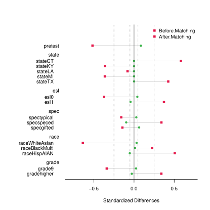
Figure 2: Covariate balance (standardized differences) before and after the propensity score match.

Figure 2 and Table 4 in the online appendix show that matching largely eliminated mean differences in pre-treatment covariates between $H=1$ and $H=0$ students. The only notable exception is in pretest scores: $H=1$ students tended to have slightly higher pretest scores than their matched comparisons with $H=0$. The p-value from an omnibus covariate balance test (Hansen and Bowers, 2008) is 0.39.

3.3 Estimating the Effects of $H$ on Posttest Scores

Let $M_{i}$ be a categorical variable denoting the matched set that $i$ belongs to. Then we may re-state the ignorability condition with reference to this match (c.f. Sales et al., 2018):

• $$\{Y(H=1),Y(H=0)\}\mathchoice{\mathrel{\hbox to0.0pt{$\displaystyle\perp$\hss}\mkern 2.0mu{\displaystyle\perp}}}{\mathrel{\hbox to0.0pt{$\textstyle\perp$\hss}\mkern 2.0mu{\textstyle\perp}}}{\mathrel{\hbox to0.0pt{$\scriptstyle\perp$\hss}\mkern 2.0mu{\scriptstyle\perp}}}{\mathrel{\hbox to0.0pt{$\scriptscriptstyle\perp$\hss}\mkern 2.0mu{\scriptscriptstyle\perp}}}H|M$$

Under matched ignorability, the difference of mean outcomes between $H=1$ and $H=0$ students within each match is unbiased for the average treatment effect for students in that match. In other words, if $\tau_{m}=\overline{Y(H=1)}-\overline{Y(H=0)}$ is the average effect in match $m$, then $\hat{\tau}_{m}=\bar{Y}_{M=m,H=1}-\bar{Y}_{M=m,H=0}$ is an unbiased estimate of $\tau_{m}$, where $\bar{Y}_{M=m,H=h}$ is the average observed outcome for subjects in match $m$ with hint level $h\in\{0,1\}$.

Weighted means of those estimated treatment effects, of the form

$$\hat{\tau}_{w}=\sum_{m}w_{m}\hat{\tau}_{m}/\sum_{m}w_{m}$$ (3)

estimate aggregate treatment effects in the sample. To estimate the average effect of $H$ for all subjects, set $w_{m}=n_{1m}+n_{0m}$, where $n_{1m}$ and $n_{0m}$ are the number of $H=1$ and $H=0$ subjects in match $m$, respectively. Alternatively, setting $w_{m}=n_{1m}$ estimates the the “treatment on the treated,” or TOT, effect—the average effect of $H$ on those subjects for whom $H=1$. Weights $w_{m}=(1/n_{1m}+1/n_{0m})^{-1}$ are “OLS” or “precision” (c.f. Schochet et al., 2015); the estimate using these weights is equal to the coefficient on $H$ from an ordinary least squares (OLS) regression of $Y$ on $H$ and a set of dummy variables for $M$. Under standard OLS assumptions, precision weights minimize the standard error of the weighted mean estimator.

Table 2 gives treatment effect estimates, standard errors, and confidence intervals under these three weighting schemes. All three sets of standard errors and confidence intervals used the heteroskedasticity-robust “HC3” sandwich estimator (Zeileis, 2004). The three estimates all roughly agree that being a high hint user decreases posttest scores by around 0.15 standard deviations. That is, they suggest that requesting hints hurts posttest scores.

The similarity of the three estimates boosts our confidence, if only slightly. The ATE and TOT estimates refer to different groups of students—ATE estimates an average effect for the entire treatment group, whereas TOT estimates an effect for high hint users. Had these been very different, one might wonder why the effect of hint requests varies so much between high and low hint users, and if that suggests selection bias. The OLS estimate downweights matched sets with many more $H=1$ than $H=0$ students or vice-versa, relative to matched sets with several of both. (Recall that such imbalanced matched sets were the result of the decision to include every subject in the analysis.) It is larger in magnitude and much less noisy than the other two estimates.

				Sensitivity Intervals
Weights	Estimate	Std. Error	CI	[Pretest]	[Ethnicity]
OLS	-0.18	0.04	[-0.25,-0.10]	[-0.41,0.06]	[-0.30,-0.05]
ATE	-0.12	0.05	[-0.23,-0.02]	[-0.45,0.20]	[-0.29,0.04]
TOT	-0.14	0.06	[-0.25,-0.03]	[-0.47,0.19]	[-0.31,0.03]

Table 2: Estimates, standard errors, and sensitivity analysis of the weighted average effect of hint usage on posttest scores, under different weighting schemes.

3.4 Sensitivity Analysis: Assessing the Role of Unmeasured Confounding

None of these estimates addressed the possibility of confounding from unmeasured covariates; instead, they relied on matched ignorability. To account for the possibility of unmeasured confounding, we conducted a sensitivity analysis following the method of Hosman et al. (2010). This method imagines a hypothetical missing covariate $U$ and estimates how the the omission of $U$ alters the estimate and its standard error. The result is a “sensitivity interval” (c.f. Rosenbaum, 2002) that, with 95% confidence, contains the true effect accounting for both sampling uncertainty and uncertainty due to possible confounding. $U$ is characterized by two sensitivity parameters: $\rho^{2}$ is the squared partial correlation between $U$ and $Y$, after accounting for the observed covariates in the model, and $T_{Z}$ is the t-statistic for the coefficient on $U$ from an ordinary least squares regression of $H$ on $U$ and the observed covariates. These sensitivity parameters may be benchmarked by estimating their counterparts when observed covariates are left out of the model.

The last two columns of Table 2 give sensitivity intervals for each of the three weighted average treatment effects. The column of Table 2 labeled “[Pretest]” accounts for the possible omission of a covariate $U$ that, at most, predicts $Y$ and $H$ as well as do pretest scores. The resulting sensitivity intervals are quite wide, including both large negative effects as well as substantial positive effects. In fact, pretest is the most important of our observed covariates; it is the observed covariate whose omission would cause the most bias. This is unsurprising, since pretests are generally considered to be the most important covariate to measure, and studies that include pretest measures often reproduce experimental estimates (e.g. Cook et al., 2008, 2009). Therefore, a sensitivity analysis considering an omitted covariate as important as pretest scores may be too pessimistic. On the other hand, it is likely that pretest scores do not fully capture between-student variance in academic ability; that is, there may be important components of prior ability (such as the ability to learn algebra) that are correlated with hint requests and posttest scores but not reflected in pretest scores. Hypothetical measurements of these components could, perhaps, constitute unobserved covariates with similar or greater importance than observed pretest scores.

A more optimistic scenario is reflected in the final column of Table 2. That column gives sensitivity intervals for the omission of a covariate that, at most, predicts $Y$ and $H$ as well as ethnicity dummy variables, the second most important of our observed covariates. These sensitivity intervals are also wide, but the interval corresponding to OLS weights is entirely negative.

The conclusion is that the omission of a confounder as important as ethnicity indicators cannot explain the estimated OLS-weighted ATE. Allowing for the possible omission of such a covariate, the results suggest that requesting a large number of hints hurts students’ posttest scores. The size of the effect may be as small as 5% of a standard deviation or as large as 30% of a standard deviation.

4 Mediation Analysis

The goal of causal mediation analysis is to decompose a treatment effect into an “indirect” or “mediated” effect and a “direct” effect. The indirect effect captures the component of the effect that is due to the mediator: the treatment affected the outcome by affecting the mediator, which itself, in turn, affected the outcome. Assignment to the treatment condition allowed students to request many hints during their work—how did the wide availability of hints affect their posttest scores? The direct effect is the component of the overall effect that operates via other mechanisms. For instance, how would assignment to CTA1 affect posttest scores were hints more limited?

The method we present here builds on the results from the observational study in the previous section. In fact, in our analysis estimating indirect effects requires no more data than the observational study. Estimating direct effects requires, additionally, data from the control group: posttest scores and (ideally) baseline covariates. The randomization of the intervention in the RCT now plays an important role in identification, since the effects of the intervention on both hint usage and posttest scores are at issue; the fact that the control group does not have access to the program likewise plays a crucial role. Finaly, the assumption of no unmeasured confounding remains important.

It is worth noting here that conducting mediation analysis requires measuring or positing a value of the mediator in the control arm of the study. We know that CTA1 hints were not available to the control group, so we set $H=0$ for all members of the control group. However, other facets of log data may not be coherently defined in the control group; for instance, students’ proclivity to master the skills of one CTA1 section before moving on to the next (Sales and Pane, 2019a) or teachers’ practice of reassigning students to new CTA1 sections (Sales and Pane, 2020). In cases such as these, the mediation framework may not apply.

The following subsection reviews the formal definitions of direct and indirect effects. Subsection 4.2 discusses identification, and 4.3 and 4.4 discuss estimation of indirect and direct effects, respectively.

4.1 Review: Defining Direct and Indirect Effect

Express a subject’s potential outcomes as a function of two variables, treatment assignment $Z$ and hint requests $H$: $Y(Z,H)$. Now, if $Z$ and $H$ are both binary, as in our example, subjects each have four potential outcomes:

$$Y(0,0);\;Y(1,0);\;Y(0,1);\;Y(1,1)$$

representing the outcomes they would exhibit were they assigned to control and requested few hints, assigned to treatment and requested few hints, assigned to control and requested many hints, or assigned to treatment and requested many hints, respectively. In the CTA1 trial, however, the potential outcome $Y(0,1)$ is meaningless: students in the control group had no access to CTA1, and therefore could not request hints. This will be an important factor going forward.

Since $H$ is itself affected by treatment assignment, it too has potential values:

$$H(0);\;H(1)$$

representing the hints that would be requested under treatment and control. In the CTA1 study, $H(0)=0$ for all subjects.

Combining potential values for $Y$ and for $H$ yields the fundamental building blocks of causal mediation analysis (e.g. VanderWeele, 2015). Let $Y(z,H(z^{\prime}))$ represent the outcome that a subject would express given treatment assignment $z$, but the hint behavior that he or she would have expressed under assignment $z^{\prime}$. When $z=z^{\prime}$, the original two potential outcomes for $Y$ emerge: $Y(1,H(1))=Y(Z=1)$ is the outcome exhibited under the treatment, when $H$ takes its potential treatment value; similarly, $Y(0,H(0))=Y(Z=0)$. On the other hand, $Y(1,H(0))$ and $Y(0,H(1))$ are strictly counterfactual. $Y(1,H(0))$ gives the outcome value that would result for a subject assigned to the treatment condition but who nevertheless requested hints as he or she would have under control. $Y(0,H(1))$ gives the potential outcome for a subject assigned to control but who nevertheless requested hints as he or she would have under treatment. This last quantity is problematic in our case, since $H(1)$ can take the value 1, and as we have seen $Y(0,1)$ is undefined.

This framework facilitates precise definitions of direct and indirect effects; in fact, there are two versions of each (e.g. Imai et al., 2011):

$$\delta(1) =Y(1,H(1))-Y(1,H(0))$$

$$\delta(0) =Y(0,H(1))-Y(0,H(0))$$

are the indirect effects, contrasting potential outcomes when $H$ varies as it would with varying treatment assignment, but holding the assignment itself constant at either 1 or 0.

$$\xi(1) =Y(1,H(1))-Y(0,H(1))$$

$$\xi(0) =Y(1,H(0))-Y(0,H(0))$$

represent the direct effects: holding the value of $H$ constant, either at its potential value under treatment or control, while varying treatment assignment. The total treatment effect, $Y(1,H(1))-Y(0,H(0))$, can then be decomposed in two ways: as $\delta(1)+\xi(0)$ or as $\delta(0)+\xi(1)$. These decompositions can potentially reveal the role hints play in the CTA1 treatment effect: $\delta(1)$ gives the extent to which assignment to CTA1 affects a student’s posttest score by (possibly) causing him or her to request many hints. $\xi(0)$ gives the effect of assignment to CTA1 if hints were, perhaps counterfactually, held at their control level, $H=0$.

Rather than attempt to estimate individual direct and indirect effects $\xi_{i}$ and $\delta_{i}$, our goal will be to estimate their means, $\mathbb{E}\xi$ and $\mathbb{E}\delta$.

4.2 Identification of Direct and Indirect Effects

Since the potential outcome $Y(0,1)$ is undefined in the CTA1 hints study, any expression (potentially) including $Y(0,1)$ is also undefined; this includes $\delta(0)$ and $\xi(1)$. Indeed, since hint behavior is unobserved in the control group altogether, conventional approaches to mediation analysis do not apply. Further, were we to operationalize hint behavior as a continuous variable, as may seem natural, mediation analysis in this case would also be nearly impossible. This is because students assigned to the control group requested exactly zero hints, whereas merely 5 members of the treatment group requested no hints over the course of the study, and these students barely used the tutor at all. That being the case, the data provide little to no information about the distribution of potential outcomes when the software is used but no hints are requested.

Dichotomizing hint requests into $H$ provides a way forward. Since the experimental design ensures that $H(0)=0$, we have that $Y(1,H(0))\equiv Y(1,0)$; this potential outcome is observed for subjects in the treatment arm with $H=0$. As above, $Y(0,H(0))=Y(0,0)$ and $Y(1,H(1))$ are the observed outcomes for subjects in the control and treatment arms, respectively. Therefore, we observe each of the potential outcomes in the definitions of $\delta(1)$ and $\xi(0)$ for at least some non-trivial portion of subjects in the study sample.

Of course, $H=0$ means something different in the two treatment arms: in the treatment group $H=0$ typically means requesting some hints, but not many, whereas subjects in the control group request exactly zero hints. One way to make sense of mediational estimands involving $H$ is to imagine an experiment in which students are assigned to different values of $H$. 70% of students in the treatment group are randomly assigned to $H=1$ and 30% to $H=0$. This assignment constrains $\bar{h}$, the proportion of problems on which they may request hints, so that if $H_{i}=0$, $\bar{h}_{i}$ is constrained to be less than 0.6, but if $H_{i}=1$ $\bar{h}_{i}$ must be greater than or equal to 0.6. In contrast, all students in the control group are assigned $H=0$ and $\bar{h}=0$.

Average potential outcomes $\mathbb{E}Y(1,H(1))$ and $\mathbb{E}Y(0,H(0))$ are identified due to the randomization of $Z$, but estimating $\mathbb{E}Y(1,H(0))$ requires imputing the potential outcome $Y(1,0)$ for treated subjects with $H_{i}=1$. However, it turns out that the matching estimators from Section 3 already solved this problem: under matched ignorability, within matched sets, $Y(1,0)$ is independent of $H$, implying that $\mathbb{E}[Y(1,0)|M,H=1]=\mathbb{E}[Y(1,0)|M,H=0]$. That suggests imputations

$$\hat{Y}_{i}(1,0)=\begin{cases}Y_{i}&H_{i}=0\\ \bar{Y}_{M=m_{i},H=0}&H_{i}=1\end{cases}$$ (4)

That is, when $Z_{i}=1$ and $H_{i}=0$, no imputation is necessary, since $Y_{i}(1,0)=Y_{i}$, the observed outcome. When $Z_{i}=1$ and $H_{i}=1$, impute the average of the observed outcomes from the $H=0$ subjects matched to $i$ for $Y_{i}(1,0)$. Matched ignorability implies that the imputations will be unbiased.

4.3 Estimating Log Data Indirect Effects

Since $\mathbb{E}\delta(1)$ involves only $Z=1$ potential outcomes, and $H(0)=0$ is known based on the study design, $\mathbb{E}\delta(1)$ may be estimated using data from the treatment group only.

Using the imputations from (4), we estimate $\mathbb{E}\delta(1)$ as

$$\widehat{\mathbb{E}\delta(1)}=\widehat{\mathbb{E}Y(Z=1)}-\widehat{\mathbb{E}Y(1,0)}=\frac{1}{n_{T}}\displaystyle\sum_{i:Z_{i}=1}Y_{i}-\hat{Y}_{i}(1,0)$$

where $n_{T}=\sum_{i}Z_{i}$, the number of subjects in the treatment group. Since $Y_{i}=\hat{Y}_{i}(1,0)$ whenever $H_{i}=0$, the summand is non-zero only when $H_{i}=1$. Further, note that when multiple $H=1$ subjects share a matched set, they also share imputations $\hat{Y}(1,0)$. Re-writing $\widehat{\mathbb{E}\delta(1)}$ in terms of matched sets $M=m$,

$$\widehat{\mathbb{E}\delta(1)} =\frac{1}{n_{T}}\displaystyle\sum_{m}\displaystyle\sum_{i:H_{i}=1,M_{i}=m}Y_{i}-\bar{Y}_{M=m_{i},H=0}$$

$$=\frac{1}{n_{T}}\displaystyle\sum_{m}n_{1m}(\bar{Y}_{M=m_{i},H=1}-\bar{Y}_{m=m_{i},H=0})$$

$$=\frac{1}{n_{T}}\displaystyle\sum_{m}n_{1m}\hat{\tau}_{m}=\frac{\sum_{i}H_{i}}{n_{T}}\widehat{TOT}$$ (5)

where $n_{1m}$ and $\hat{\tau}_{m}$ were defined in Section 3.3 as the number of $H=1$ subjects in match $m$ and the difference in the sample mean of $Y$ between $H=1$ and $H=0$ subjects in match $m$, respectively, and $\widehat{TOT}$ is the TOT estimate, (3) with $w_{m}=n_{1m}$. The upshot of (5) is that under matched ignorability, $\mathbb{E}\delta(0)$ can be estimated as the TOT times the proportion of the treatment group with $H=1$.

Actually, this relationship between $\mathbb{E}\delta(0)$ and the TOT holds in the population, regardless of how the TOT is estimated. This is because when $H_{i}=0$, then $H_{i}(1)=H_{i}(0)=0$, so the individual direct effect $\delta_{i}(1)=0$, and when $H_{i}=1$, $\delta_{i}(1)=Y_{i}(H=1)-Y_{i}(H=0)$, the effect of $H$ on $Y$. Therefore,

$$\mathbb{E}\delta(1)=\mathbb{E}\mathbb{E}[\delta(1)|H]=\mathbb{E}[\delta(1)|H=1]Pr(H=1)=TOTPr(H=1)$$

In the hint study, the definition of $H$ implies that $Pr(H=1)=\sum_{i}H_{i}/n_{T}=$0.3. Therefore, our estimate of the average indirect effect is $\widehat{\mathbb{E}\delta(1)}=$0.3$\widehat{TOT}$. In Table 2, we estimated the TOT as -0.14 with a standard error of 0.06. That implies an average indirect effect of -0.04, with a standard error of 0.02.

It is worth repeating that these estimates assume matched ignorability—no confounding between $H$ and $Y$ within matched sets. With this important caveat, this analysis suggests that the wide availability of a hints actually lowers the treatment effect, that CTA1 works not because of hints, but despite them.

4.4 Estimating Log Data Direct Effects

What would the effect be were all students to request few hints? To answer that question, we estimate average direct effects, $\mathbb{E}[\xi(0)]=\mathbb{E}[Y(1,H(0))-Y(0,H(0))]=\mathbb{E}[Y(1,0)-Y(0,0)]$. In principal, this could be estimated as the difference in sample means of $\hat{Y}(1,0)$ in the treatment group and observed $Y=Y(0,0)$ in the control group. In general, if we let

$$\tilde{Y}\equiv Z\hat{Y}(1,0)+(1-Z)Y(0,0)$$

then we can estimate $\mathbb{E}[\xi(0)]$ as the ATE of treatment assignment $Z$ on $\tilde{Y}$. Just like estimates of the ATE of $Z$ on $Y$, this estimate should account for the experimental design: a paired, group-randomized trial with students clustered in schools and schools randomized within pairs.

For the sake of simplicity, we will use an OLS regression estimator, with cluster-robust standard errors (Pustejovsky and Tipton, 2018), clustered at the school level. (Since in Section 3 subjects were matched within schools, school-level cluster-robust standard errors also account for the dependence of $\hat{Y}(1,0)$ between matched treated students.) Specifically, we regress:

$$\tilde{Y}_{i}=\alpha_{p[i]}+\widehat{\mathbb{E}[\xi(0)]}Z_{i}+\epsilon_{i}$$ (6)

where $\alpha_{p[i]}$ is a fixed intercept for the randomization pair of subject $i$’s school and $\epsilon_{i}$ is a regression error. Using the clubSandwich package in R (Pustejovsky, 2018) to estimate standard errors, and 95% confidence intervals, we estimated a direct effect of 0.14$\pm$0.25. Adding covariates to the regression (6) estimates a direct effect of 0.18$\pm$0.21.

Table 3 summarizes our mediation results: assuming matched ignorability, assignment to CTA1 increases student test scores despite the availability of hints (an indirect effect of -0.04 standard deviations), and the effect due to CTA1’s other mechanisms is 0.18.

Effect	Estimate	CI
Avg. Indirect Effect ($\mathbb{E}\delta(1)$)	-0.04	[-0.07,-0.01]
Avg. Direct Effect ($\mathbb{E}\xi$)	0.14	[-0.10,0.39]
Avg. Direct Effect, covariate adjusted ($\mathbb{E}\xi$)	0.18	[-0.03,0.39]

Table 3: Estimated effects in mediation analysis.

5 Principal Stratification

In a principal stratification (PS; Frangakis and Rubin, 2002) analysis, the researcher stratifies all students in the RCT—in both the treatment and control arms—based on how they would use the software were they (perhaps counterfactually) assigned to the treatment condition. The goal is to estimate the average effect of assignment to the treatment condition separately in each stratum. In our analysis, we imagine that each student has his or her own proclivity to request hints, when possible: if assigned to treatment, each student would tend to request hints at a different rate. How does the effect of assignment to the CTA1 condition vary with these proclivities? Would the benefit of being assigned to the CTA1 condition be higher or lower for students who would tend to request more hints than for those who would tend to request fewer?

In an RCT, identification of these varying effects relies on randomization of treatment assignment, rather than on assumptions about unmeasured confounders. Unlike the observational study or mediation analysis, PS in an RCT requires no assumptions about unmeasured confounding. PS analysis requires data on outcomes (e.g. posttest scores) in both treatment arms, as well as data on implementation. In classical PS (e.g. Page, 2012; Feller et al., 2016b), the intermediate variable, implementation, is discrete or categorical, leading to discrete strata. Other approaches (Gilbert and Hudgens, 2008; Jin and Rubin, 2008, e.g.) allow the intermediate variable to be continuous. The method we use here is based on Sales and Pane (2019a), in which the variable defining principal strata is latent—specifically, the “ability” parameter in (1). For this approach, implementation is measured with a series of binary measurements for each student, with each measurement taken from a specific problem or section. Other implementation data structures may call for different measurement models. Finally, covariates may not be strictly necessary for PS, but they can be extremely helpful.

Below, we describe a Bayesian PS model fit in one step. However, the full process of PS analysis is a much more involved procedure. After a formal introduction in Subsection 5.1, Subsection 5.2 describes a set of sub-models for student hint requests, posttest scores, and treatment effects. Ideally, each of these models should be carefully tailored to each data application, and each must be rigorously tested. Model checking includes examination of residual data plots, fake data simulation, and fitting a range of alternative specifications in a sensitivity analysis. More details for checking PS models can be found in Sales and Pane (2019a) and Sales and Pane (2019b), and for Bayesian models in general in Gelman et al. (2014) and McElreath (2020).

5.1 Principal Effects for EdTech Log Data

In the PS approach, $Y(0)=Y(Z=0)$ and $Y(1)=Y(Z=1)$ are the only potential outcomes for $Y$. As in mediation analysis, hint behavior has potential outcomes as well. Specifically, the rate at which as student requests hints, $\bar{h}$, has potential values $\bar{h}(1)$ and $\bar{h}(0)$, though only $\bar{h}(1)$ is relevant in the CTA1 study.

The goal of PS is to estimate “principal effects”:

$$\tau(r)=\mathbb{E}[Y(1)-Y(0)|\bar{h}(1)=r]$$

This is the treatment effect for subjects who would request hints at level $\bar{h}(1)=r$, if assigned to the treatment condition. The goal of PS is to estimate the relationship between $\bar{h}(1)$ and treatment effects; this contrasts with the observational study and mediation analysis whose goal was the relationship between $\bar{h}$ and posttest scores. Notably, although $Y(0)$ and $\bar{h}(1)$ and $Y(0)$ are never simultaneously observed, the $\tau(r)$ estimand does not depend on any strictly-counterfactual outcomes. Unlike, say, $Y(0,H(1))$, $Y(0)$ and $Y(1)$ are each truly potential—they would each occur under treatment assignments $Z=0$ and $Z=1$. That said, estimating $\tau(r)$ requires estimation of $\mathbb{E}[Y(0)|\bar{h}(1)]$, the average of $Y(0)$ over a subset of the sample that is unobserved and must be inferred. For this reason, $\tau(r)$ is only partially identified (e.g. Mealli et al., 2016); even with an infinite sample, principal effect estimates will still contain uncertainty.

In previous sections $\bar{h}$ was dichotomized into $H$; such dichotomization is not necessary here. However, $\bar{h}$ has some disadvantages as a continuous measure of hint usage (Sales and Pane, 2019a). For one, since it is essentially a sample mean over a subset of each student’s worked problems, much of its variance is driven by the total number of problems students worked—in particular, its extreme values belong to those students who barely used the tutor at all. Further, it does not account for varying difficulty of the tutor’s problems. In Section 2.3.1, we showed that dichotomized $\bar{h}$ largely agrees with a dichotomized version of a more sophisticated measure of hint usage. However, when modeling hint usage continuously, the correspondence may not hold (see Sales and Pane, 2019a, for a more complete discussion).

For those reasons, we modeled hint usage at the problem level, with equation (1), but with two important differences. First, a conceptual difference: the $\eta$ in (1) was replaced by $\eta(1)$, indicating that it is measuring potential hint usage—the hint usage a student would exhibit were he or she assigned to the treatment condition. Whereas $\eta$ is only defined for students assigned to the treatment condition, $\eta(1)$ is defined for all the students in the study. Second, a modeling difference: instead of the normal mixture model (2), we modeled $\eta(1)$ with a normal regression model. With this change, the PS estimand became

$$\tau(r)=\mathbb{E}[Y(1)-Y(0)|\eta(1)=r]$$

the treatment effect for students whose potential hint usage, if assigned to the treatment condition, $\eta(1)=r$. A full treatment of this variant of PS, including a discussion of identification and estimation, may be found in Sales and Pane (2019a).

5.2 Specifying PS Models

Estimating $\tau(r)$ required estimating $\mathbb{E}[Y(0)|\eta(1)=r]$, despite the fact that hint requests are never observed at the same time as $Y(0)$ (in fact $\eta(1)$ isn’t directly observed in either the treatment or control group). However, among those students with $Z=1$, hint requests are observed and the conditional distribution $\eta(1)|\bm{x}$ is identified; because of randomization of $Z$, these inferences extend to the control group as well (Feller et al., 2016b).

Our approach to PS estimation is model-based and Bayesian, following Jin and Rubin (2008), Schwartz et al. (2011) and others. The PS model consists of three sub-models, all depending on a vector of parameters $\bm{\theta}$ that contains regression coefficients, variance components, and treatment effects. The sub-models are: $p(h;\eta(1),\bm{\theta})$, giving the distribution of actual hint requests as a function of $\eta(1)$, $p(\eta(1)|\bm{x},\bm{\theta})$ giving the distribution of $\eta(1)$ conditional on covariates, and $p(Y|\eta(1),Z,\bm{x},\bm{\theta})$ giving the conditional distribution of outcomes. With these three models in hand, and a prior distribution $p(\bm{\theta})$, posterior inference for $\bm{\theta}$ proceeds based on the following structure:

$$p(\bm{\theta}|\bm{Y},\bm{Z}, \bm{X},\{\bm{h}_{i}\}_{i:Z_{i}=1})\propto$$

$$p(\bm{\theta}) \displaystyle\prod_{i:Z_{i}=1}\int p(Y_{i}|\bm{x}_{i},Z=1,\bm{\theta},\eta(1))p(\bm{h}_{i}|\eta(1),\bm{\theta})p(\eta(1)|\bm{x}_{i},\bm{\theta})d\eta(1)$$

$$\times \displaystyle\prod_{i:Z_{i}=0}\int p(Y_{i}|\bm{x}_{i},Z=0,\bm{\theta},\eta(1))p(\eta(1)|\bm{x}_{i},\bm{\theta})d\eta(1).$$ (7)

where $\bm{h}_{i}$ is the vector of hint request data for subject $i$, ranging over all challenging problems. In other words, we estimate parameters by integrating over unknown (latent) $\eta(1)$ values, using the distribution of $\eta$ estimated in the treatment group. This is, in essence, an infinite mixture distribution, with outcome distribution $p(Y|\cdot)$ and mixing proportions $p(\eta(1)|\cdot)$. Unlike in typical PS setups, $\eta(1)$ is unobserved for both $Z=1$ and $Z=0$ treatment groups, but is estimated using both $\bm{h}$ and $\bm{x}$ in the treatment group, but only $\bm{x}$ in the control group.

First, students’ proclivity to request hints is measured by the $\eta$ parameter in (1). In the next level, $\eta(1)$ is modeled as a function of baseline covariates $\bm{x}$:

$$\eta(1)|\left(\bm{x}_{i},\bm{\theta}\right)\sim\mathcal{N}\left(\bm{x_{i}}\bm{\beta}+\epsilon^{tch}_{t[i]}+\epsilon^{scl}_{s[i]},\sigma\right)$$ (8)

where $\bm{\beta}$ is a vector of coefficients. Since students were nested within teachers, who were nested within schools, we included normally-distributed school ($\epsilon^{scl}$) and teacher ($\epsilon^{tch}$) random intercepts. The covariates in the model, $\bm{x}_{i}$, were detailed in Table 1; preliminary model checking suggested including a quadratic term for pretest, which was added as a column of $\bm{x}_{i}$.

We modeled students’ posttest scores $Y$ as conditionally normal:

$$Y|\left(Z_{i},\bm{x}_{i},\bm{\theta},\eta(1)\right)\sim\mathcal{N}\left(\gamma_{0b[i]}+\bm{x}_{i}^{T}\bm{\gamma}+a\eta(1)+Z_{i}(b_{0}+b_{1}\eta(1))+\zeta^{tch}_{t[i]}+\zeta^{scl}_{s[i]},\omega_{Z[i]}\right)$$ (9)

where $\gamma_{0b[i]}$ is a fixed effect for $i$’s randomization block, $\bm{\gamma}$ are the covariate coefficients, and $\zeta^{tch}$, and $\zeta^{scl}$ are normally-distributed teacher and school random intercepts. The residual variance $\omega$ varies with treatment assignment $Z$; this captures measurement error in $Y$, treatment effect heterogeneity that is not linearly related to $\eta(1)$, and other between-student variation in $Y$ that is not predicted by the mean model.

Model (9) implies that treatment effects are linear in $\eta(1)$, $\mathbb{E}[Y(1)-Y(0)|\eta(1)]=\tau({\eta(1)})=b_{0}+b_{1}\eta(1)$

While more complex models for $\tau(\eta(1))$ are theoretically possible (for instance, Jin and Rubin (2008) uses a quadratic model), in our experience non-linear effect models do not perform as well in model checks as the the linear model.

Covariates $\bm{X}$ were standardized prior to fitting. Prior distributions for the block fixed effects $\beta^{Y}_{b}$ and covariate coefficients $\bm{\beta^{Y}}$ and $\bm{\beta^{M}}$ were normal with mean zero and standard deviation 2; priors for treatment effects and the coefficient on $\eta(1)$ were standard normal. The rest of the parameters received standard reference priors. In all cases, we expected true parameter values to be much smaller in magnitude than the prior standard deviation.

5.3 Estimating Principal Effects

Figure 1 shows the estimated linear function $\hat{\tau}(r)$. The left panel shows the CTA1 treatment effect, $Y(1)-Y(0)$ as $r=\tau(1)$ varies; the black line shows the estimate (i.e. posterior mean) and the magenta lines are random draws from the posterior distribution, showing estimation uncertainty. Seventy-five percent of posterior draws of the slope of the $\hat{\tau}(\cdot)$ function were positive, implying a posterior probability of 0.75 that students who asked for hints with greater regularity benefited more from the CTA1 curriculum. A 95% highest-density credible interval for the slope parameter is [-0.06,0.12]. Therefore, the data are consistent with either a slightly negative or a positive relationship between hint requests and treatment effects, but the latter is more likely.

The right hand panel plots one posterior draw of $\eta(1)$ alongside observed outcomes $Y$. The figure also includes estimated regression lines for the two treatment groups. Although, as observed in Sections 3 and 4, $\eta(1)$ is anticorrelated with $Y$, the slope is steeper in the control group than in the treatment group. The distance between the two regression lines is the treatment effect, which grows with $\eta(1)$.

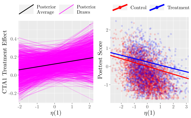
Figure 1: Results from the PS model. On the left, the estimated CTA1 treatment effect is plotted against hint request proclivity $\eta(1)$. The black line is the posterior mean, and the red lines are random posterior draws. The right panel plots observed posttest scores against one random draw of $\eta(1)$, along with regression lines for the treatment and control groups.

These results suggest that students who, under treatment, would tend to ask for hints on challenging problems, are most responsive to treatment.

6 Comparing Strategies

In the case discussed here, the observational study and mediation approaches appear to give the opposite conclusion from principal stratification—matching and mediation suggest that excessive hint requests hurt students’ posttest scores, while principal stratification suggests that students who request more hints may experience higher treatment effects. This section will compare and contrast the three methods in terms of their necessary identification assumptions, their model fitting mechanics, and interpretation of their results.

The fundamental difference between the observational study and mediation approach, on the one hand, and principal stratification on the other, is in the role of $H$, the intermediate variable. An observational study or mediation analysis treats $H$ as a causal agent, an intervention or exposure that affects $Y$. In mediation analysis, it is also an (intermediate) outcome, affected by $Z$. The approach of principal stratification is quite nearly opposite: $H$ is not an exposure, that “happens to” subjects, but rather its potential value $H(1)$ is a characteristic of the subjects. Observed $H$ reveals what was there all along.

6.1 Causal Identification

Observational studies, and mediation analyses that build on them, require ignorability assumptions such as Strong Ignorability or Matched Ignorability. These may be particularly problematic in our study, since students who are more likely to request hints are also more likely to struggle with the material. We addressed this concern in three ways: first, we focused our attention on the set of problems in the tutor in which students either requested a hint or made an error, second, with propensity score matching, and third with sensitivity analysis. None of these approaches is bulletproof—they each require further assumptions about how students request hints. Eliminating problems in which students showed no signs of struggling is likely to reduce the association between hint requests and underlying academic ability, but not eliminate it. For instance, stronger students may be better able to figure out a difficult problem without access to hints or error feedback than weaker students. Matching depends both on the adequacy of the observed covariates to capture baseline differences between $H=0$ and $H=1$ students, and the sensitivity analyses we performed assumed that any un-measured covariate would predict $H$ and $Y$ no better than pretest or ethnicity indicators, respectively. These assumptions are impossible to verify from the data at hand; instead, judging their plausibility requires a keen understanding of student practice within the tutor.

Mediation analysis builds on the matching design, and requires the same ignorability assumption; it must additionally overcome the hurdle of the almost complete lack of overlap between hint request behavior in the control group (i.e. zero) and in the treatment group. Under our approach of dichotomizing hint request behavior, mediation analysis is essentially a way to interpret the results of the observational study in the context of the full RCT.

In contrast, no ignorability assumptions are necessary for principal stratification. However, principal stratification estimators require modeling assumptions—most problematically, $p(Y|\bm{x},Z=0,\bm{\theta},\eta(1))$ of (7), the model for $Y(0)$ conditional on $\eta(1)$, $\bm{x}$, and parameters $\bm{\theta}$. While any model specification can, and should, be checked against observed data, this process can only narrow the space of acceptable models, it cannot be used to determine the correct form of $p(Y|\bm{x},Z=0,\bm{\theta},\eta(1))$. This is because $Y(0)$ and $\eta(1)$ are never observed simultaneously. Therefore, it is possible for an analyst to misspecify $p(Y|\bm{x},Z=0,\bm{\theta},\eta(1))$, such that principal effect estimates are severely biased, without being able to detect the model misspecification with the data. That is, the data will typically be unable to distinguish between alternative $p(Y|\bm{x},Z=0,\bm{\theta},\eta(1))$ models that lead to qualitatively different conclusions. In practice, we make the untestable assumption that $p(Y|\bm{x},Z=0,\bm{\theta},\eta(1))$ is of the same form as $p(Y|\bm{x},Z=1,\bm{\theta},\eta(1))$.

An additional contrast of note between matching-based studies and principal stratification relates to transparency. However complex the process of devising a match may be, the resulting design is simple and clear—subjects with $H=1$ are compared against matches with $H=0$. This transparency may help researchers assess the plausibility of the match, and diagnose potential problems with resulting estimates. Though principal stratification does not depend on ignorability, it does depend on a highly intricate and parametric modeling structure. If any part of the model is sufficiently misspecified, the results may be wrong. Perhaps worse, Feller et al. (2016a) argued that even well-specified models can give severely biased estimates. Extensive model interrogation and checking is necessary for principal stratification analysis, but the complexity of the principal stratification model makes this process particularly difficult. Sales and Pane (2019a) gives some examples of potentially fruitful model checking procedures, which are also carried out in the online supplement.

6.2 Results and Interpretation

Our observational study suggested that hint requests have a negative effect: students who requested hints more often than the 70th percentile score lower on the posttest, after controlling for observed covariates. Taken at face value, this suggests that the optimal strategy is to request few, if any, hints. However, this conclusion assumes that there were no omitted confounders. An omitted confounder that is as important as pretest could explain the relationship, but an omitted confounder as important as ethnicity—our second most important covariate—could not (so long as we estimate an OLS-weighted average effect).

Mediation analysis essentially interprets the observational study result in terms of the overall CTA1 treatment effect. Specifically, the analysis in 4 showed that CTA1 affected students’ posttest scores in (at least) two opposite ways: by allowing hints, it lowered their posttest scores, but its other mechanisms increased their scores by an even greater amount.

The principal stratification analysis also found a negative correlation between hint requesting and posttest scores. Those students who request more hints are those who need more help of some form, and tend to score lower on the posttest. Fortunately, the principal stratification analysis also suggests (with probability 0.75) that these students may benefit more from CTA1 than their peers who request fewer hints. However, it is unclear whether their larger treatment effects are due to their higher rate of hint requests, or to some other related characteristic.

Can these three sets of results be reconciled? Does requesting hints help or hurt? Technically, principal stratification has nothing to say about the effect of hints—$\eta(1)$ is modeled as a student characteristic, not an intervention. (See Jin and Rubin 2008 for a nice discussion of this point.) Still, doesn’t the correlation between treatment effects and hint requests suggest that hints may be beneficial? Does that contradict the results in Sections 3 and 4 that hints requests lower students’ posttest scores? In fact, the results of the three methods can be reconciled. For instance, it may be that requesting hints indeed lowers test scores—a negative indirect effect—but that those students who are likely to request more hints also tend to experience greater direct effects. That is, it may be that the observational and mediational results are correct—that requesting hints lowers test scores—but that the principal stratification results are also correct—students who request more hints tend to experience higher treatment effects, due to other mechanisms. (Of course, the data are also consistent with the possibilities that the relationship between hint requests and treatment effects is negative, or close to zero, in which case there is less that needs to be explained.)

6.3 Choosing Between Methods

The previous discussion suggests three criteria for choosing between the three approaches we’ve discussed here. First is the question the researcher seeks to answer. In their most straightforward interpretations, principal stratification is a method for examining treatment effect heterogeneity (are students benefiting differently?), whereas mediation analysis is a method for assessing causal mechanisms (is the wide availability of hints in CTA1 beneficial to students?). That said, principal stratification may also shed light on potential causal mechanisms—if, indeed, treatment effects are higher for students who request more hints, then hints may play a role in the tutor’s effectiveness.

A second criterion is the researcher’s willingness to make ignorability assumptions. A researcher’s confidence in her understanding of a data generating process and the quality of observed covariates can translate into confidence about the results of an observational study or mediation analysis. Conversely, researchers unwilling to consider untestable ignorability assumptions will find principal stratification an attractive alternative.

The final criterion is a researcher’s comfort with complex statistical models. Researchers who are able and willing to experiment with a range of models for a dataset, and perhaps devise tests of model fit tailored to a specific problem, may be more confident in the fit of a principal stratification model. Researchers who prefer transparency and non-parametric or semi-parametric analysis may prefer matching studies.

Additional philosophical concerns come in to play as well. For instance, unlike observational studies and principal stratification, mediation analysis depends on strictly counterfactual quantities, such as $Y(0,H(1))$, that can never occur. Analogous quantities in principal stratification, such as $\mathbb{E}[Y(0)|\eta(1)]$ are unobservable, but nevertheless refer to averages of potential outcomes among actual experimental subjects. These concerns are important but beyond the scope of the current paper; for more discussion, see the citations in the introduction.

In summary: there is much to recommend the observational study approach if risks of confounding bias appear limited (due to the availability of high-quality covariates, good reason to believe variation in implementation is random or haphazard, or other factors). A wide variety of straightforward and transparent estimation techniques are available, such as the propensity score matching illustrated here. The result—the ATE of implementation on the outcome—is an intuitive estimand.

When employed, mediation analysis can contextualize the estimated implementation effect from the observational study in terms of the experiment’s overall treatment effect, enabling implementation to be interpreted as a causal mechanism.

However, where unobserved confounding is a serious threat, and complex statistical modeling (and model checking) is not a practical barrier, principal stratification may be a better choice because no ignorability assumptions are necessary.

Of course, there are approaches to modeling implementation beyond the three considered here. For instance, principal stratification based on non-parametric bounding (Miratrix et al., 2017) or randomization inference (Nolen and Hudgens, 2011) would avoid the parametric assumptions of model-based principal stratification, as would a standard moderation analysis based on predicted implementation, $\hat{\eta}(1)$ instead of partially observed $\eta(1)$. We hope that future work will develop these methods, and still others.

7 Discussion: Causal Inference and Measurement

This case study has focused on three approaches to causal modeling of hint requests during an RCT of the Cognitive Tutor program. We hope we have demonstrated some of the potential and some of the challenges that new datasets logged by online learning systems bring to these old problems.

Measurement of students’ hint request rates played a central role in all three approaches we considered. The results were largely driven by three measurement decisions. First, our decision to consider only worked Cognitive Tutor problems on which students either requested a hint or made an error (or both) reduced the relationship between hint requests and student algebra I ability. Second, our decision to dichotomize hint request rates in the observational study and mediation analysis allowed us to use of a traditional matching estimator and to identify mediational estimands. Third, our decision to use a Rasch model to measure hint usage in the principal stratification analysis accounted for differences between students in both the number and difficulty of worked CT problems.

While questions of measurement has always been important in causal inference, analysis of EdTech log data brings them to the fore. Log datasets from technology products are large, multivariate, and complex, so careful thought is necessary in order to measure implementation constructs of interest.

Even if they are motivated by methodological concerns, decisions about measurement are inherently also decisions about causal questions—estimates using different measurements answer different questions. Just as researchers must choose a causal approach, such as matching, mediation, or principal stratification, they must choose a measurement approach as well. As our case study demonstrated, these two decisions are deeply intertwined.

The size, dimension, and complexity of EdTech log data suggests some exciting opportunities for innovative combinations of measurement and causal approaches. We demonstrated the inclusion of an IRT model in principal stratification; this suggests the possibility of including other measurement models into causal estimators. Multivariate measurement models that incorporate not only hint requests, but other usage measures such as time spent, actions taken, and errors could yield deep insights about how students use EdTech products and how different usage patterns correspond to different effects. The development of these causal models will require simultaneous consideration of causal inference and measurement.

Appendix A Rasch Mixture Model of Hint Usage

To model hint requests with a mixture model, we modeled each hint request as in (1). Then, instead of modeling $\eta_{i}$ as normal, we assigned it a two-component normal mixture model:

$$\eta\sim p_{0}\mathcal{N}(\mu_{0},\sigma_{0})+(1-p_{0})\mathcal{N}(\mu_{1},\sigma_{1})$$

where we constrained $\mu_{0}<\mu_{1}$.

A.1 Stan Code

## data{
## //Sample sizes
##  int<lower=1> N; // total number of obs (long format)
##  int<lower=1> nstud; // # students
##  int<lower=1> nsec; // # sections (problems nested in sections)
##
## // indices
##  int<lower=1,upper=nstud> studentM[N]; //for each obs, which student?
##  int<lower=1,upper=nsec> section[N]; // for each obs, which section?
##
## // data data
##  int<lower=0,upper=1> hint[N]; // for each obs, was a hint requested?
##
## }
## parameters{
##
##  vector[nstud] eta; // ability parameter
##  real<lower=0,upper=1> p1; // mixing proportion
##  //ordered[2] mu;             // locations of mixture components
##  real<upper=0> mu0; //location of mixture component 0
##  vector<lower=0>[2] sigma;  // scales of mixture components
##
##  real delta[nsec]; // section difficulty parameter
##  //real<lower=0> sigSec; // scale of difficulty parameters
##
## }
## transformed parameters{
##  real<lower=0> mu1; // location of mixture component 1
##  mu1= -(1-p1)/p1*mu0;
## }
## model{
##  // logs of mixing proportions to save time
##  real log_p1=log(p1);
##  real log_p0=log(1-p1);
##
## // linear predictor for logit model
##  real linPred[N];
##
## // priors
##  sigma ~ lognormal(0, 2);
##  mu0 ~ normal(0, 2);
## // sigSec ~ lognormal(0,2);
##  p1~ beta(2,2); // I’d rather the groups have similar sizes
##
## // model for section difficulty parameters
##  delta~normal(0,3);//sigSec);
##
## // Rasch model for hint requests
##  for(i in 1:N)
##   linPred[i]= eta[studentM[i]]-delta[section[i]];
##
##  hint~bernoulli_logit(linPred);
##
##
## // mixture model for ability parameters
##  for(n in 1:nstud)
##   target += log_sum_exp(log_p0+normal_lpdf(eta[n]|mu0,sigma[1]),
## ΨΨΨlog_p1+normal_lpdf(eta[n]|mu1,sigma[2]));
##
## }

Appendix B Covariate Balance Before and After Matching

	Unmatched			Matched
	std.diff	z		std.diff	z
grade9	-0.34	-7.05	***	0.03	0.44
gradehigher	0.34	7.05	***	-0.03	-0.44
raceWhiteAsian	-0.64	-12.83	***	0.03	0.75
raceBlackMulti	0.23	4.71	***	0.01	0.24
raceHispAIAN	0.51	10.35	***	-0.05	-0.98
pretest	-0.52	-10.54	***	0.09	1.82	.
spectypical	-0.16	-3.32	***	0.03	0.48
specspeced	0.34	7.07	***	-0.10	-1.44
specgifted	-0.14	-3.03	**	0.06	1.16
esl0	-0.37	-7.70	***	0.04	0.63
esl1	0.37	7.70	***	-0.04	-0.63
stateCT	0.58	11.81	***	-0.00	0.00
stateKY	-0.36	-7.51	***	-0.00	0.00
stateLA	-0.08	-1.68	.	-0.00	0.00
stateMI	-0.36	-7.51	***	0.00	0.00
stateTX	0.43	8.77	***	0.00	0.00

Table 4: Covariate balance (standardized differences and Z-scores) before and after the propensity score match.

Appendix C Stan Code for Principal Stratification Model

C.1 Stan Code

## data{
## //Sample sizes
##  int<lower=1> nsecWorked;
##  int<lower=1> ncov;
##  int<lower=1> nstud;
##  int<lower=1> nteacher;
##  int<lower=1> nsec;
##  int<lower=1> nschool;
##  int<lower=1> npair;
##
## // indices
##  int<lower=1,upper=nteacher> teacher[nstud];
##  int<lower=1,upper=npair> pair[nstud];
##  int<lower=1,upper=nschool> school[nstud];
##  int<lower=1,upper=nstud> studentM[nsecWorked];
##  int<lower=1,upper=nsec> section[nsecWorked];
##
## // data data
##  int<lower=0,upper=1> hint[nsecWorked];
##  matrix[nstud,ncov] X;
##  int<lower=0,upper=1> Z[nstud];
##  real Y[nstud];
##
## }
## parameters{
##
##  vector[nstud] eta;
##
##  vector[ncov] betaU;
##  vector[ncov] betaY;
##
##  real a1;
##  real b0;
##  real b1;
##
##  real teacherEffY[nteacher];
##  real teacherEffU[nteacher];
##  real pairEffect[npair];
##  real schoolEffU[nschool];
##  real schoolEffY[nschool];
##  real delta[nsec];
##
##  real<lower=0> sigTchY;
##  real<lower=0> sigSclY;
##  real<lower=0> sigY[2];
##  real<lower=0> sigTchU;
##  real<lower=0> sigSclU;
##  real<lower=0> sigU;
## }
##
## model{
##  real linPred[nsecWorked];
##  vector[nstud] muY;
##  vector[nstud] muU;
##  real useEff[nstud];
##  real trtEff[nstud];
##  real sigYI[nstud];
##
##
## // hint model
##  for(i in 1:nsecWorked)
##   linPred[i]= delta[section[i]]+eta[studentM[i]];
##
##  for(i in 1:nstud){
##   useEff[i]=a1*eta[i];
##   trtEff[i]=b0+b1*eta[i];
##   muU[i]=teacherEffU[teacher[i]]+schoolEffU[school[i]];
##   muY[i]=teacherEffY[teacher[i]]+schoolEffY[school[i]]+
##          pairEffect[pair[i]]+useEff[i]+Z[i]*trtEff[i];
##   sigYI[i]=sigY[Z[i]+1];
##  }
##
##  //priors
##  betaY~normal(0,2);
##  betaU~normal(0,2);
##  pairEffect~normal(0,2);
##
##  a1~normal(0,1);
##  b0~normal(0,1);
##  b1~normal(0,1);
##
##
##  schoolEffY~normal(0,sigSclY);
##  schoolEffU~normal(0,sigSclU);
##  teacherEffU~normal(0,sigTchU);
##  teacherEffY~normal(0,sigTchY);
##
##  hint~bernoulli_logit(linPred);
##
##  eta~normal(muU+X*betaU,sigU);
##  Y~normal(muY+X*betaY,sigYI);
## }
## generated quantities{
## // int<lower=0,upper=1> hintRep[nsecWorked];
##  real Yrep[nstud];
##
## // hintRep=bernoulli_logit_rng(linPred);
##  for(i in 1:nstud)
##   Yrep[i] = normal_rng(teacherEffY[teacher[i]]+schoolEffY[school[i]]+
##             pairEffect[pair[i]]+a1*eta[i]+Z[i]*(b0+b1*eta[i])+
## Ψ    X[i,]*betaY,sigY[Z[i]+1]);
## }

Appendix D Diagnostic Plots for Principal Stratification

D.1 Posterior Predictive Density Plots

Figures 3, 4, and 5 compare the density of observed outcomes $y$ to 1000 random draws of the model-implied density, $y_{rep}$ for the full (“pooled”) sample, the treatment group, and the control group, respectively. They show a close, but not perfect, correspondence between the observed data and the model. The most noticeable difference is the left-truncation of the observed outcomes—the lower tail is lighter than would be expected from a normal distribution—suggesting floor effects on the posttest not considered in the model. The misspecification appears similar in both treatment groups. A model accounting for floor effects may fit the data more closely. These plots were made with the bayesplot package [Gabry, 2016] in R.

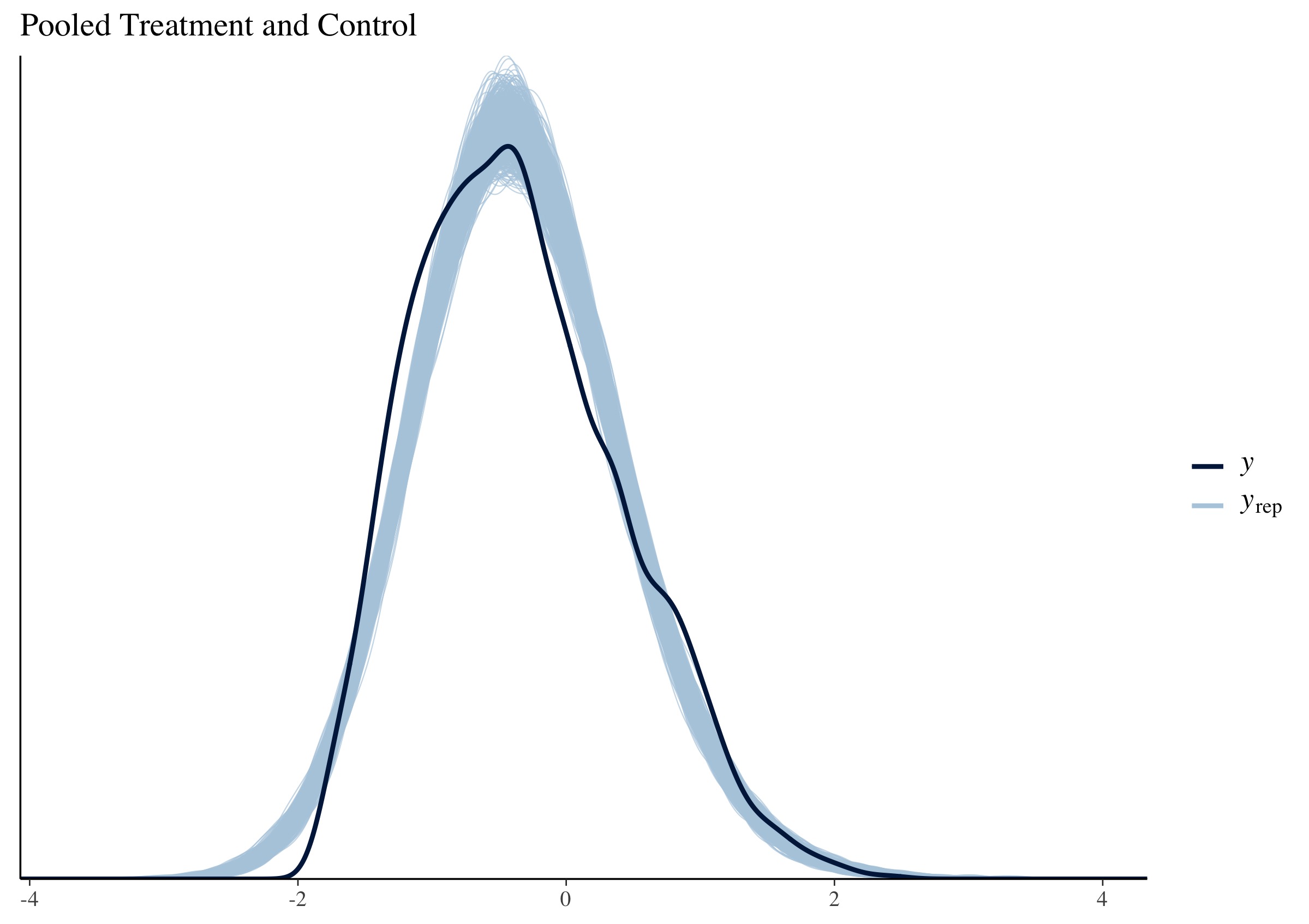
Figure 3: A comparison of the estimated density of observed outcomes $y$ with 1000 random draws of the model-implied outcome density, for the full dataset.

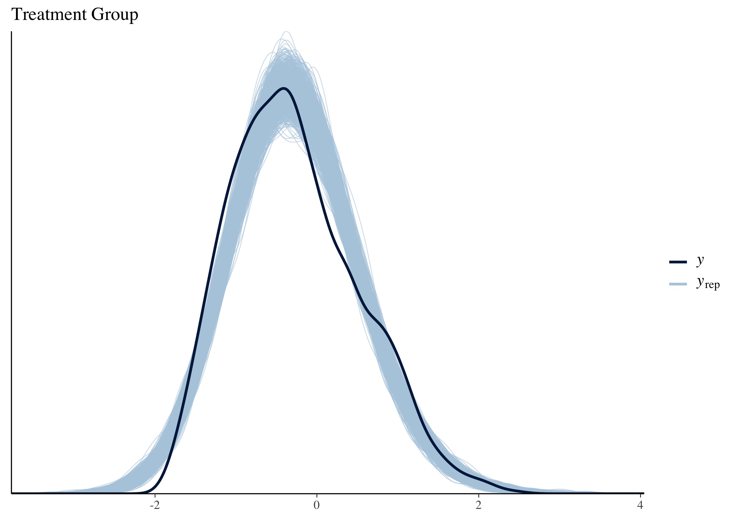
Figure 4: A comparison of the estimated density of observed outcomes $y$ with 1000 random draws of the model-implied outcome density, for the treatment group.

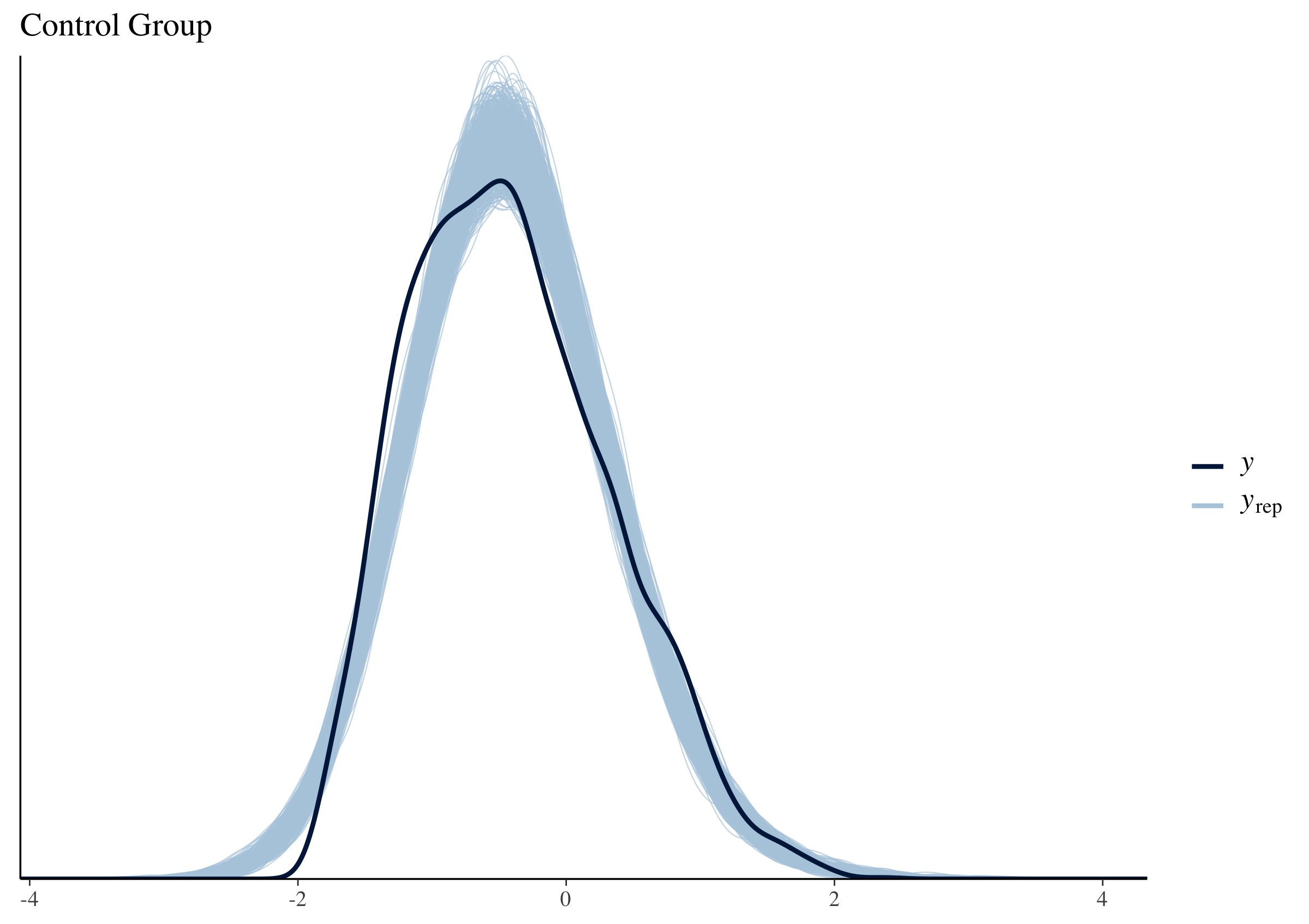
Figure 5: A comparison of the estimated density of observed outcomes $y$ with 1000 random draws of the model-implied outcome density, for the control group.

D.2 Residual Plots

Figures 6, 7, and 8 plot residuals $Y_{i}-\hat{Y}_{i}$ against fitted values $\hat{Y}_{i}$ for the full sample, the treatment group, and the control group, respectively. Here, fitted values $\hat{Y}$ are posterior means—averages over all of the draws from the model. The residual plots reflect the floor effects apparent in the posterior predictive density plots—a subset of points appears to fall along a straight line in the bottom left of the plot. Otherwise, little structure is apparent.

Figure 9 assesses the hint sub-model, (1) and (8) by comparing the binned model-implied probabilities of hint requests on individual worked problems to residuals—the differences between these probabilities and the proportions of worked problems within each bin that resulted in an actual hint request [c.f. Gelman et al., 2014]. Nine random draws from the posterior distribution are shown. Little structure is apparent in the binned residuals, suggesting that the model for hint requests fits well.

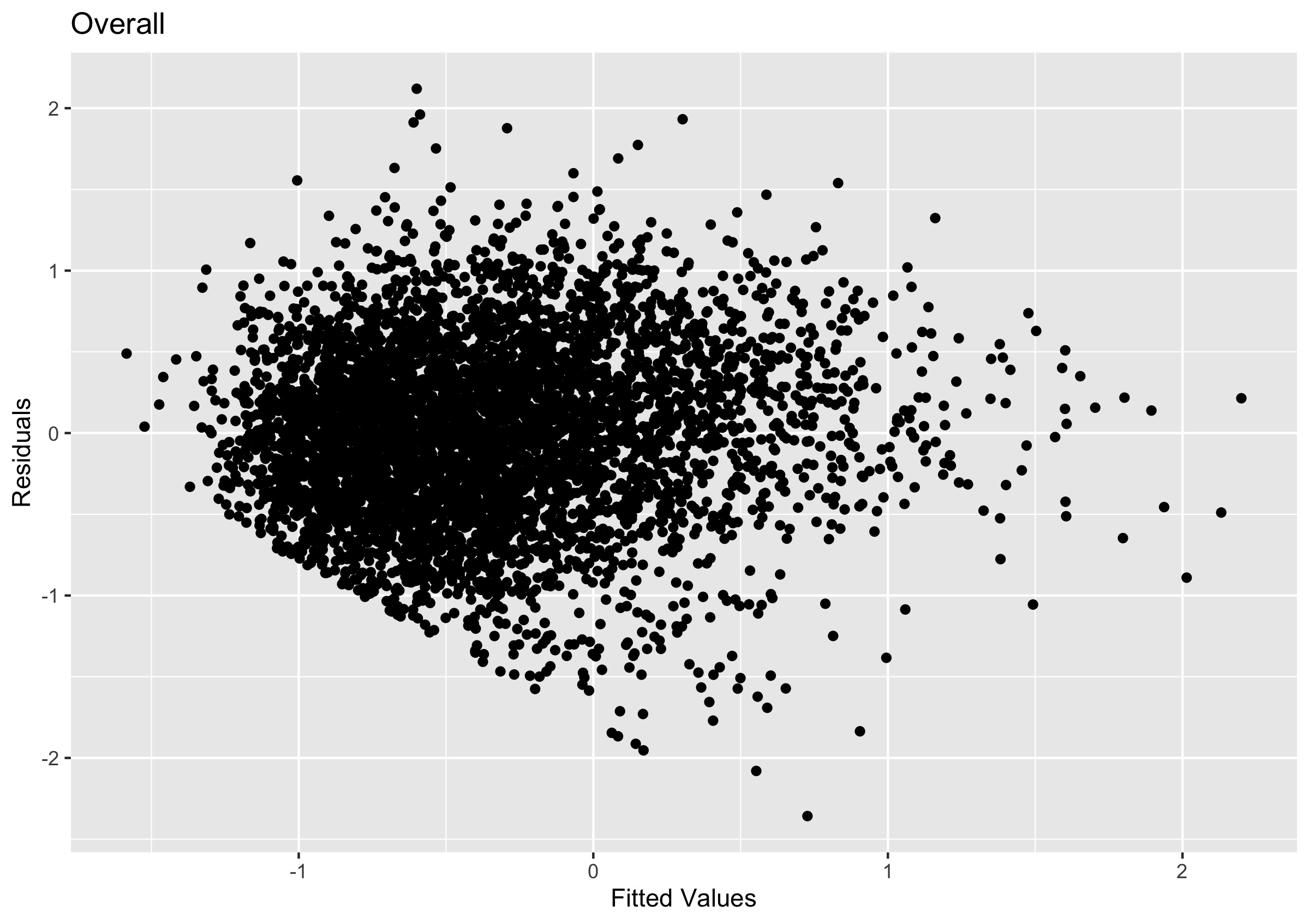
Figure 6: A residual plot for the full sample.

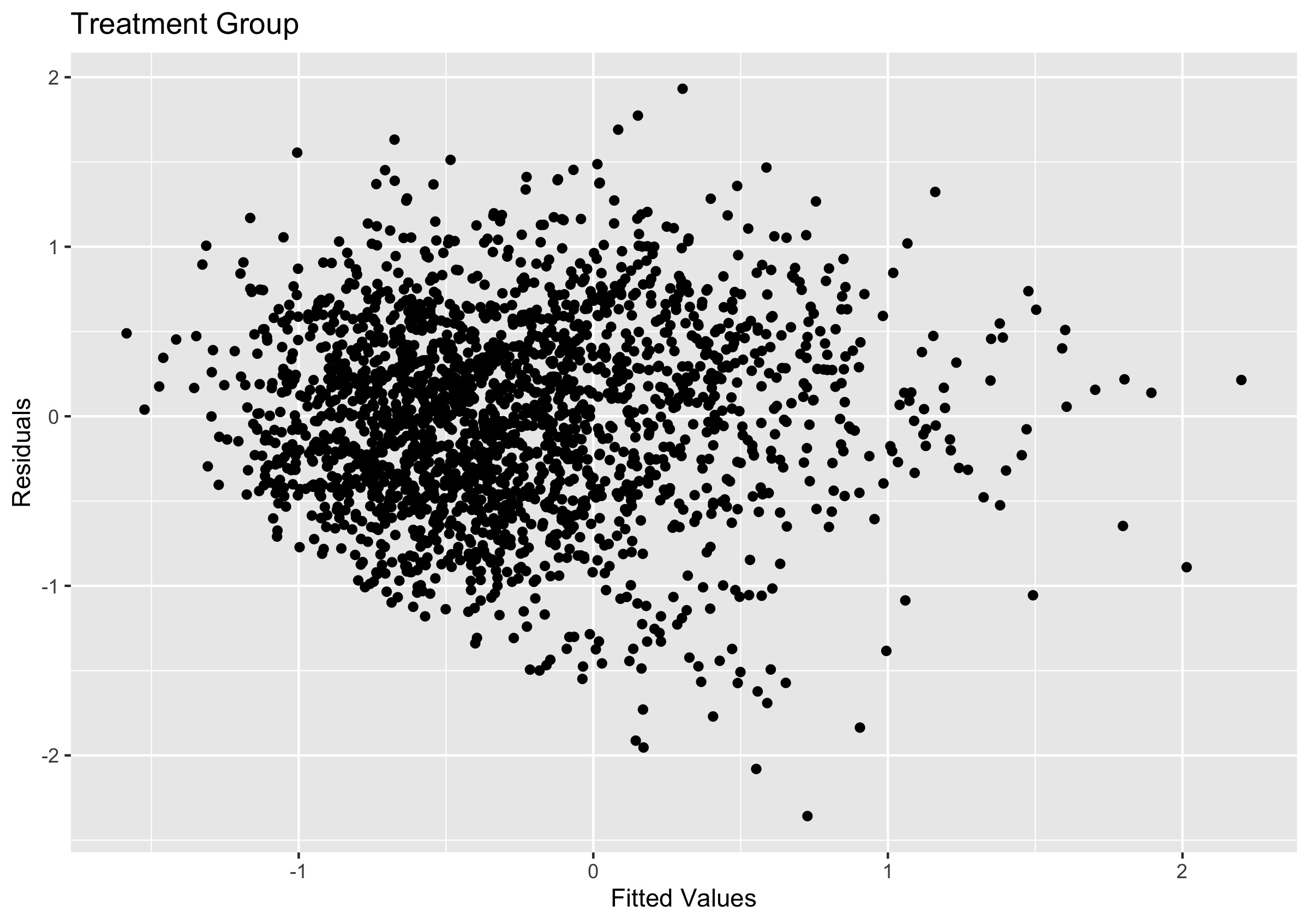
Figure 7: A residual plot for the treatment group.

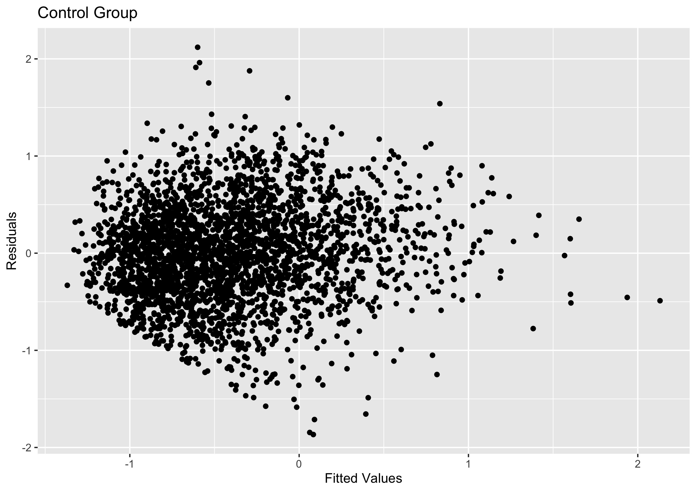
Figure 8: A residual plot for the control group

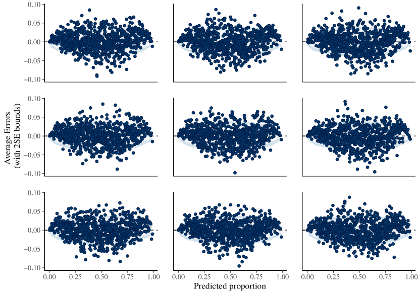
Figure 9: Binned residual plot for model of hint requests.

D.3 Fake Data Simulation

Figure 10 implements a model assessment for principal stratification suggested in Sales and Pane [2019a]. In this method, we replace data from the real control group with duplicated outcome and covariate data from the treatment group (now re-labeled as control). In other words, each member of the treatment group appears in the dataset twice, once in the “treatment” group and once in the “control” group. Only the “treatment” observations are linked with hint data. We also re-labeled teachers and schools in the “control” group so that the were distinct from the corresponding labels in the “treatment” group.

The upper left plot of 10 fits the same principal stratification model described in Section 5.2 to the new dataset, in which there is exactly no effect. In the other three panels of 10, the model is fit to the fake data with simulated treatment effects added: a random treatment effect uncorrelated with $\eta(1)$, a treatment effect linear in $\eta(1)$ (as we estimated) and a treatment effect quadratic in $\eta(1)$. These fake datasets contain the same quirks as the real treatment group data (and hence the same model misspecification) but with known treatment effects. In the first three plots, our model recovered the truth, albeit with considerable uncertainty. In the bottom left (quadratic) plot, our model could not recover the true relationship between $\eta(1)$ and $\tau$ because we modeled $\tau$ as linear in $\eta(1)$. However, the model did not estimate a spurious positive or negative associations between $\eta(1)$ and $\tau$.

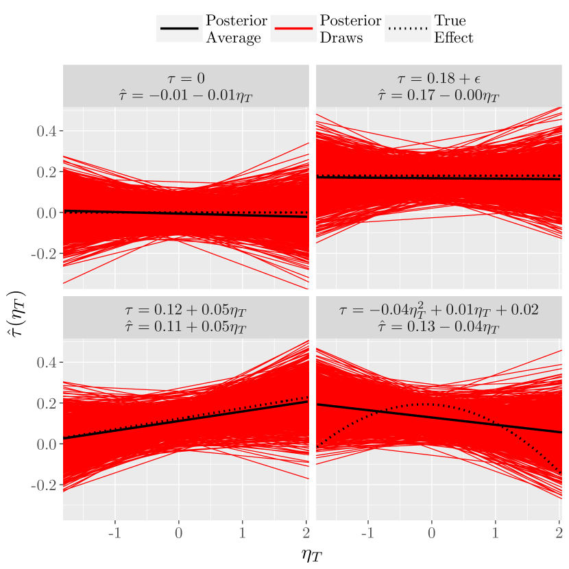
Figure 10: Comparisons between principal stratification model estimates and true treatment effects when the treatment group is replicated (without corresponding hint request data) and relabeled as control, and (clockwise from upper left) no treatment effect, a random treatment effect uncorrelated with $\eta(1)$, a treatment effect linear in $\eta(1)$, or a treatment effect quadratic in $\eta(1)$ is added to the original treatment group.

References

- Aleven et al. [2016] Vincent Aleven, Ido Roll, Bruce M McLaren, and Kenneth R Koedinger. Help helps, but only so much: Research on help seeking with intelligent tutoring systems. International Journal of Artificial Intelligence in Education, 26(1):205–223, 2016.
- Anderson [2013] John R Anderson. The architecture of cognition. Psychology Press, 2013.
- Anderson et al. [1985] John R Anderson, C Franklin Boyle, and Brian J Reiser. Intelligent tutoring systems. Science(Washington), 228(4698):456–462, 1985.
- Anderson et al. [1995] John R Anderson, Albert T Corbett, Kenneth R Koedinger, and Ray Pelletier. Cognitive tutors: Lessons learned. The journal of the learning sciences, 4(2):167–207, 1995.
- Bates et al. [2015] Douglas Bates, Martin Mächler, Ben Bolker, and Steve Walker. Fitting linear mixed-effects models using lme4. Journal of Statistical Software, 67(1):1–48, 2015. doi: 10.18637/jss.v067.i01.
- Beck et al. [2008] Joseph E Beck, Kai-min Chang, Jack Mostow, and Albert Corbett. Does help help? introducing the bayesian evaluation and assessment methodology. In International Conference on Intelligent Tutoring Systems, pages 383–394. Springer, 2008.
- Bowers et al. [2017] Jake Bowers, Mark Fredrickson, and Ben Hansen. RItools: Randomization Inference Tools (Development Version), 2017. URL https://github.com/markmfredrickson/RItools. R package version 0.2-0.
- Caliendo and Kopeinig [2008] Marco Caliendo and Sabine Kopeinig. Some practical guidance for the implementation of propensity score matching. Journal of economic surveys, 22(1):31–72, 2008.
- Cook et al. [2008] Thomas D Cook, William R Shadish, and Vivian C Wong. Three conditions under which experiments and observational studies produce comparable causal estimates: New findings from within-study comparisons. Journal of Policy Analysis and Management: The Journal of the Association for Public Policy Analysis and Management, 27(4):724–750, 2008.
- Cook et al. [2009] Thomas D Cook, Peter M Steiner, and Steffi Pohl. How bias reduction is affected by covariate choice, unreliability, and mode of data analysis: Results from two types of within-study comparisons. Multivariate Behavioral Research, 44(6):828–847, 2009.
- Escueta et al. [2017] Maya Escueta, Vincent Quan, Andre Joshua Nickow, and Philip Oreopoulos. Education technology: an evidence-based review. Technical report, National Bureau of Economic Research, 2017.
- Fancsali et al. [2020] S.E Fancsali, K Holstein, M Sandbothe, S Ritter, B.M McLaren, and V. Aleven. Towards practical detection of unproductive struggle. Proceedings of the 21st International Conference on Artificial Intelligence in Education, 2020.
- Feller et al. [2016a] Avi Feller, Evan Greif, Luke Miratrix, and Natesh Pillai. Principal stratification in the twilight zone: Weakly separated components in finite mixture models. arXiv preprint arXiv:1602.06595, 2016a.
- Feller et al. [2016b] Avi Feller, Todd Grindal, Luke Miratrix, Lindsay C Page, et al. Compared to what? variation in the impacts of early childhood education by alternative care type. The Annals of Applied Statistics, 10(3):1245–1285, 2016b.
- Frangakis and Rubin [2002] Constantine E Frangakis and Donald B Rubin. Principal stratification in causal inference. Biometrics, 58(1):21–29, 2002.
- Gabry [2016] Jonah Gabry. bayesplot: Plotting for Bayesian Models, 2016. URL https://CRAN.R-project.org/package=bayesplot. R package version 1.1.0.
- Gelman et al. [2014] Andrew Gelman, John B Carlin, Hal S Stern, David B Dunson, Aki Vehtari, and Donald B Rubin. Bayesian data analysis, volume 2. CRC press Boca Raton, FL, 2014.
- Gilbert and Hudgens [2008] Peter B Gilbert and Michael G Hudgens. Evaluating candidate principal surrogate endpoints. Biometrics, 64(4):1146–1154, 2008.
- Goldin et al. [2012] Ilya M Goldin, Kenneth R Koedinger, and Vincent Aleven. Learner differences in hint processing. International Educational Data Mining Society, 2012.
- Hansen [2004] Ben B Hansen. Full matching in an observational study of coaching for the sat. Journal of the American Statistical Association, 99(467):609–618, 2004.
- Hansen [2011] Ben B. Hansen. Propensity score matching to extract latent experiments from nonexperimental data: A case study. In Neil Dorans and Sandip Sinharay, editors, Looking Back: Proceedings of a Conference in Honor of Paul W. Holland, chapter 9, pages 149–181. Springer, 2011.
- Hansen and Bowers [2008] Ben B. Hansen and Jake Bowers. Covariate balance in simple, stratified and clustered comparative studies. Statistical Science, 23(2):219–236, 2008.
- Hansen and Klopfer [2006] Ben B. Hansen and Stephanie Olsen Klopfer. Optimal full matching and related designs via netwrk flows. Journal of Computational and Graphical Statistics, 15(3):609–627, 2006.
- Hirano and Imbens [2004] Keisuke Hirano and Guido W Imbens. The propensity score with continuous treatments. Applied Bayesian modeling and causal inference from incomplete-data perspectives, 226164:73–84, 2004.
- Ho et al. [2007] Daniel E. Ho, Kosuke Imai, Gary King, and Elizabeth A. Stuart. Matching as nonparametric preprocessing for reducing model dependence in parametric causal inference. Political Analysis, 15:199–236, 2007. URL http://gking.harvard.edu/files/matchp.pdf.
- Hong [2015] Guanglei Hong. Causality in a social world: Moderation, mediation and spill-over. John Wiley & Sons, 2015.
- Hosman et al. [2010] Carrie A Hosman, Ben B Hansen, Paul W Holland, et al. The sensitivity of linear regression coefficients’ confidence limits to the omission of a confounder. The Annals of Applied Statistics, 4(2):849–870, 2010.
- Imai et al. [2011] Kosuke Imai, Luke Keele, Dustin Tingley, and Teppei Yamamoto. Unpacking the black box of causality: Learning about causal mechanisms from experimental and observational studies. American Political Science Review, 105(4):765–789, 2011.
- Israni et al. [2018] Anita Israni, Adam C Sales, and John F Pane. Mastery learning in practice: A (mostly) descriptive analysis of log data from the cognitive tutor algebra i effectiveness trial, 2018.
- Jin and Rubin [2008] Hui Jin and Donald B Rubin. Principal stratification for causal inference with extended partial compliance. Journal of the American Statistical Association, 103(481):101–111, 2008.
- Jo [2008] Booil Jo. Causal inference in randomized experiments with mediational processes. Psychological Methods, 13(4):314, 2008.
- Kalton [1968] Graham Kalton. Standardization: A technique to control for extraneous variables. Applied Statistics, pages 118–136, 1968.
- Koedinger and Aleven [2007] Kenneth R Koedinger and Vincent Aleven. Exploring the assistance dilemma in experiments with cognitive tutors. Educational Psychology Review, 19(3):239–264, 2007.
- Koedinger et al. [2012] Kenneth R Koedinger, Albert T Corbett, and Charles Perfetti. The knowledge-learning-instruction framework: Bridging the science-practice chasm to enhance robust student learning. Cognitive science, 36(5):757–798, 2012.
- Leon and Hedeker [2005] Andrew C Leon and Donald Hedeker. A mixed-effects quintile-stratified propensity adjustment for effectiveness analyses of ordered categorical doses. Statistics in medicine, 24(4):647–658, 2005.
- Li and Zhou [2017] Wei Li and Xiao-Hua Zhou. Identifiability and estimation of causal mediation effects with missing data. Statistics in medicine, 36(25):3948–3965, 2017.
- Lopez et al. [2017] Michael J Lopez, Roee Gutman, et al. Estimation of causal effects with multiple treatments: a review and new ideas. Statistical Science, 32(3):432–454, 2017.
- McElreath [2020] Richard McElreath. Statistical rethinking: A Bayesian course with examples in R and Stan. CRC press, 2020.
- McKendree [1990] Jean McKendree. Effective feedback content for tutoring complex skills. Human-computer interaction, 5(4):381–413, 1990.
- Mealli and Mattei [2012] Fabrizia Mealli and Alessandra Mattei. A refreshing account of principal stratification. The international journal of biostatistics, 8(1), 2012.
- Mealli et al. [2016] Fabrizia Mealli, Barbara Pacini, and Elena Stanghellini. Identification of principal causal effects using additional outcomes in concentration graphs. Journal of Educational and Behavioral Statistics, 41(5):463–480, 2016.
- Miratrix et al. [2017] Luke Miratrix, Jane Furey, Avi Feller, Todd Grindal, and Lindsay C Page. Bounding, an accessible method for estimating principal causal effects, examined and explained. Journal of Research on Educational Effectiveness, pages 1–30, 2017.
- Neyman [1923] Jersey Neyman. Sur les applications de la théorie des probabilités aux experiences agricoles: Essai des principes. Roczniki Nauk Rolniczych, 10:1–51, 1923.
- Nolen and Hudgens [2011] Tracy L Nolen and Michael G Hudgens. Randomization-based inference within principal strata. Journal of the American Statistical Association, 106(494):581–593, 2011.
- Paas and Van Merriënboer [1994] Fred GWC Paas and Jeroen JG Van Merriënboer. Variability of worked examples and transfer of geometrical problem-solving skills: A cognitive-load approach. Journal of educational psychology, 86(1):122, 1994.
- Page [2012] Lindsay C Page. Principal stratification as a framework for investigating mediational processes in experimental settings. Journal of Research on Educational Effectiveness, 5(3):215–244, 2012.
- Pane et al. [2014] John F Pane, Beth Ann Griffin, Daniel F McCaffrey, and Rita Karam. Effectiveness of cognitive tutor algebra i at scale. Educational Evaluation and Policy Analysis, 36(2):127–144, 2014.
- Pavlik Jr et al. [2009] Philip I Pavlik Jr, Hao Cen, and Kenneth R Koedinger. Performance factors analysis–a new alternative to knowledge tracing. Proceedings of the 2009 conference on Artificial Intelligence in Education, pages 531––538, 2009.
- Pearl [2011] Judea Pearl. Principal stratification–a goal or a tool? The international journal of biostatistics, 7(1):1–13, 2011.
- Pustejovsky [2018] James Pustejovsky. clubSandwich: Cluster-Robust (Sandwich) Variance Estimators with Small-Sample Corrections, 2018. URL https://CRAN.R-project.org/package=clubSandwich. R package version 0.3.2.
- Pustejovsky and Tipton [2018] James E Pustejovsky and Elizabeth Tipton. Small-sample methods for cluster-robust variance estimation and hypothesis testing in fixed effects models. Journal of Business & Economic Statistics, 36(4):672–683, 2018.
- R Core Team [2016] R Core Team. R: A Language and Environment for Statistical Computing. R Foundation for Statistical Computing, Vienna, Austria, 2016. URL https://www.R-project.org/.
- Rasch [1993] Georg Rasch. Probabilistic models for some intelligence and attainment tests. ERIC, 1993.
- Rosenbaum [2002] P.R. Rosenbaum. Observational studies. Springer, 2002.
- Rosenbaum and Rubin [1983] P.R. Rosenbaum and D.B. Rubin. The central role of the propensity score in observational studies for causal effects. Biometrika, 70(1):41–55, 1983.
- Rubin [1978] Donald B Rubin. Bayesian inference for causal effects: The role of randomization. The Annals of statistics, pages 34–58, 1978.
- Rubin [2004] Donald B Rubin. Direct and indirect causal effects via potential outcomes. Scandinavian Journal of Statistics, 31(2):161–170, 2004.
- Sales and Pane [2020] Adam Sales and John Pane. The effect of teachers reassigning students to new cognitive tutor sections. In Proceedings of the 13th International Conference on Educational Data Mining. International Educational Data Mining Society, 2020.
- Sales et al. [2016] Adam Sales, Asa Wilks, and John Pane. Student usage predicts treatment effect heterogeneity in the cognitive tutor algebra i program. In Proceedings of the 9th International Conference on Educational Data Mining. International Educational Data Mining Society, pages 207–214, 2016.
- Sales and Pane [2019a] Adam C Sales and John F Pane. The role of mastery learning in an intelligent tutoring system: Principal stratification on a latent variable. The Annals of Applied Statistics, 13(1):420–443, 2019a.
- Sales and Pane [2019b] Adam C Sales and John F Pane. Principal stratification for intelligent tutors: A tutorial. 2019b. URL https://github.com/adamSales/tutorial/blob/master/paper.pdf.
- Sales et al. [2018] Adam C Sales, Ben B Hansen, and Brian Rowan. Rebar: Reinforcing a matching estimator with predictions from high-dimensional covariates. Journal of Educational and Behavioral Statistics, 43(1):3–31, 2018.
- Schochet et al. [2015] Peter Z Schochet et al. Statistical theory for the rct-yes software: Design-based causal inference for rcts. Princeton, NJ: Mathematica Policy Research, 2015.
- Schwartz et al. [2011] Scott L Schwartz, Fan Li, and Fabrizia Mealli. A bayesian semiparametric approach to intermediate variables in causal inference. Journal of the American Statistical Association, 106(496):1331–1344, 2011.
- Shadish and Steiner [2010] William R Shadish and Peter M Steiner. A primer on propensity score analysis. Newborn and Infant Nursing Reviews, 10(1):19–26, 2010.
- Singh et al. [2011] Ravi Singh, Muhammad Saleem, Prabodha Pradhan, Cristina Heffernan, Neil T Heffernan, Leena Razzaq, Matthew D Dailey, Cristine O’Connor, and Courtney Mulcahy. Feedback during web-based homework: the role of hints. In International Conference on Artificial Intelligence in Education, pages 328–336. Springer, 2011.
- Stekhoven and Buehlmann [2012] Daniel J. Stekhoven and Peter Buehlmann. Missforest - non-parametric missing value imputation for mixed-type data. Bioinformatics, 28(1):112–118, 2012.
- Sweller and Cooper [1985] John Sweller and Graham A Cooper. The use of worked examples as a substitute for problem solving in learning algebra. Cognition and instruction, 2(1):59–89, 1985.
- VanderWeele [2015] Tyler VanderWeele. Explanation in causal inference: methods for mediation and interaction. Oxford University Press, 2015.
- VanderWeele [2008] Tyler J VanderWeele. Simple relations between principal stratification and direct and indirect effects. Statistics & Probability Letters, 78(17):2957–2962, 2008.
- VanderWeele [2011] Tyler J VanderWeele. Principal stratification–uses and limitations. The international journal of biostatistics, 7(1):1–14, 2011.
- VanderWeele [2012] Tyler J VanderWeele. Comments: Should principal stratification be used to study mediational processes? Journal of research on educational effectiveness, 5(3):245–249, 2012.
- Zeileis [2004] Achim Zeileis. Econometric computing with hc and hac covariance matrix estimators. Journal of Statistical Software, 11(10):1–17, 2004. URL http://www.jstatsoft.org/v11/i10/.