Multi-robot Dubins Coverage with Autonomous Surface Vehicles

Abstract

In large scale coverage operations, such as marine exploration or aerial monitoring, single robot approaches are not ideal, as they may take too long to cover a large area. In such scenarios, multi-robot approaches are preferable. Furthermore, several real world vehicles are non-holonomic, but can be modeled using Dubins vehicle kinematics. This paper focuses on environmental monitoring of aquatic environments using Autonomous Surface Vehicles (ASVs). In particular, we propose a novel approach for solving the problem of complete coverage of a known environment by a multi-robot team consisting of Dubins vehicles. It is worth noting that both multi-robot coverage and Dubins vehicle coverage are NP-complete problems. As such, we present two heuristics methods based on a variant of the traveling salesman problem—$k$-TSP—formulation and clustering algorithms that efficiently solve the problem. The proposed methods are tested both in simulations to assess their scalability and with a team of ASVs operating on a 200 $\textbf{km}^{2}$ lake to ensure their applicability in real world.

I INTRODUCTION

This paper addresses the problem of covering a large area for environmental monitoring with multiple Dubins vehicles. Coverage is a task common to a variety of fields. The application areas can be classified based on the scale of operations, by the necessity to ensure the coverage of all available free space (termed complete coverage), and by whether there is prior knowledge of the environment. From small scale household tasks such as vacuum cleaning and lawn mowing to large scale operations such as automation in agriculture, search and rescue, environmental monitoring, and humanitarian de-mining, coverage is a key component. See [1, 2] for in-depth surveys. Finding a solution to the coverage problem means planning a trajectory for a mobile robot in a way that an end-effector, often times the body of the robot, passes over every point in the available free space. Employing multiple robots can reduce the coverage time cost, and, in hazardous conditions, such as humanitarian de-mining, increase the robustness by completing the task even in the event of accidental “robot deaths.” The use of multiple robots however, increases the logistical management and the algorithmic complexity.

Covering an unknown environment, termed online coverage [3], focuses on ensuring that no part is left uncovered and on minimizing repeat coverage. In contrast, when covering a known environment, the focus is on performing the task as efficiently as possible [4]. As mentioned above, another classification is between ensuring complete coverage versus, in limited time, ensuring that the most interesting areas are covered [5]. Furthermore, the scale of the environment in conjunction with the speed and endurance of the robot(s) classify the coverage task as small, medium, or large scale. For example, a flying vehicle with $30\text{\,}\mathrm{min}$ battery life and an average speed of $40\text{\,}\mathrm{km}\text{/}\mathrm{h}$ can cover a trajectory of $20\text{\,}\mathrm{km}$, while an autonomous surface vehicle (ASV), moving at $10\text{\,}\mathrm{kn}$ ($5\text{\,}\mathrm{m}\text{/}\mathrm{s}$) for five hours will travel approximately $90\text{\,}\mathrm{km}$.

Figure 1: Three autonomous surface vehicles during coverage experiments at Lake Murray, SC, USA.

In this paper we focus on the monitoring of aquatic environments. The vehicles of choice are ASVs that were custom-made at the University of South Carolina (see Figure 1). Aquatic environments, in general, require large scale operations. For example, one of the testing grounds used—Lake Murray—has a surface of over $200\text{\,}{\mathrm{km}}^{2}$. Many ASVs, similar to fixed wing aircraft, are governed by Dubins vehicle kinematics [6]; i.e., Dubins vehicles cannot turn in place. More formally, a Dubins vehicle is defined as a vehicle which may only follow line segments and arcs with radius greater than some specified minimum with non-negative velocity, i.e., they may not back up. Recent work [7, 8] presented an efficient approach to cover an area by a single Dubins vehicle. We extend the proposed algorithm to multiple robots based on recent work on multi-robot coverage [9] for holonomic robots. This work ensures a more efficient division of labor between robots, particularly for large scale environments. Efficiency is measured as a combination of the utilization of the robots and the reduction of the maximum coverage cost. The idea is that robots are limited battery life; as such, the workload should be evenly distributed. We present two methods. In the first one, the efficient path produced by the algorithm proposed by Lewis et al. [8] is divided to approximately equal parts, in terms of path length, and each part is assigned to a different robot. In the second method, the target area is divided into equal parts, based on the team size, and then the single robot algorithm [8] is applied to each area.

Experimental results from several simulated experiments show that indeed the utilization of the robots is maximized and the maximum coverage cost is minimized. Moreover, the approach is scalable to a large number of robots. Field trials with a single robot, a team of two, and a team of three ASVs, demonstrated the feasibility of the proposed approach with real robots executing plans generated by the planner and highlighted several practical challenges.

The next section discusses related work for the complete coverage problem using either single or multi-robot systems. Section III presents the problem statement and, in the following section, an outline of the proposed approach is discussed. The experimental setup is presented in Section V together with results from simulation and from the deployment of a team of ASVs in Lake Murray, SC, USA. Finally, a discussion of lessons learned together with future directions of this work concludes the paper in Section VI.

II RELATED WORK

There are numerous ways to formulate coverage, including static or dynamic coverage, complete or partial, offline or online [1, 2]. In addition, there are many different approaches to tackle such a problem, such as defining it as graph partitioning problem, performing region-based decomposition, or defining it as sub-modular optimization problem [10, 2].

When prior information about the environment is available as a map, the coverage is called offline [1]. One of the approaches widely used in offline coverage algorithms is based on area decomposition. Choset [11] proposed a cellular decomposition technique, called boustrophedon decomposition (BCD). In his work, the coverage are is decomposed into obstacle free cell. A lawnmower pattern is typically executed to cover each cell. Other approaches were also used for decomposing areas based on Morse decomposition [12] or grid-based decomposition [13].

Some of the grid-based methods to single robot coverage were adapted for multi-robot systems as well [14, 15, 16, 17]. The robustness and efficiency of the systems proposed by that body of work depend on the resolution of the input representation. Because the size of each cell is typically based on the size of the sensor footprint, the coverage becomes more challenging in environments with many obstacles, as the footprint size increases.

Polynomial time algorithms were proposed for solving single robot coverage using a boustrophedon decomposition based approach [18, 4]. In contrast to the original algorithm, in these approaches, the problem is represented as the Chinese postman problem (CPP). The latter is a graph routing problem, of finding a minimum-cost closed tour that visits each edge at least once. Edmonds and Johnson [19] found a polynomial-time solution for CPP.

When considering the coverage problem for robots with turning constraints, a simple boustrophedon coverage plan may introduce wasted time—that is, time spent out of the region of interest because of the constraints and thus not actually covering. The Dubins vehicle is a common robot model in coverage problems, and Savla, Bullo, and Frazzoli [20] consider a control-theoretic solution. In our work, however, we provide an algorithmic approach to minimizing the path length by minimizing the time spent not actively covering because of the motion constraints.

Reducing traversal time by considering motion constraints is not a new idea in coverage. Both Huang [21] and Yao [22] minimize the path length by using motion constraints in their environmental decompositions. Both of them, however, seek to reduce the amount of rotation required by the robot, while we optimize the solution by carefully selecting how the robot transitions from covering to not-covering.

This idea is related to the traveling salesman problem (TSP) with Dubins curve constraints, called Dubins traveling salesman problem. In [23, 24], the Dubins TSP is defined as metric TSP with the additional constraint that paths between nodes must adhere to a minimum turn radius necessary for the covering vehicle’s transition between nodes.

Some of the presented methods based on cellular decomposition were also designed for multi-robot systems [3], assuming restricted communication. Avellar et al. [25] present a multi-robot coverage approach that operates in two phases: decomposing the area into line-sweeping rows, based on which a complete graph is constructed to be used in the second phase, where the vehicle routing problem [26] is solved. Field trials with Unmanned Aerial Vehicles (UAV) showed that their proposed approach provides minimum-time coverage. However, that algorithm is only applicable for obstacle free environments.

In our previous work [9], we presented a communication-less multi-robot coverage algorithm based on efficient single robot coverage. Even if the proposed methods demonstrate better performance on robots utilization and almost optimal work division, the robots utilization is dependent on the number of obstacles in the area. As in that work clustering is based on boustrophedon cells, a small number of obstacles will result in small number of cells, and consequently less clusters per regions. Note that, however, the solution generated did not take into account any kinematic constraints of the robots.

A large body of work in multi-robot systems assumes that there is some form of communication between the robots [27]. Some of them came up with alternative implicit communication means, such as trail of other robots [28, 29, 30]. Nevertheless, this type of communication is impractical in aquatic or aerial environments.

The graph routing problems such as TSP and CPP have also their definition for multiple routes: finding $k$ routes that visit non overlapping vertices of the graph, such that the union of those clusters are the exact set of vertices in the TSP case. This problem is called $k$-TSP problem. When edges are considered instead of vertices, the problem is called $k$-CPP. Both these problems and their variations were shown to be NP-complete [31].

In this paper, differently from the current state of the art, we address multi-robot coverage for Dubins vehicles, for which no solution is readily available. In the following section, the problem is formally defined.

III PROBLEM STATEMENT

The Dubins multi-robot coverage problem can be formulated as follows. We assume to have $k$ homogeneous robots, with no communication capabilities, equipped with a sensor with fixed-size footprint $s$, and with Dubins constraints—namely, the robots have a minimum turning radius $r$, that constrains the robots to follow line segments and arcs with radius greater than $r$, and they cannot drive in reverse. Such robots are deployed in a $2$D-bounded area of interest region $\mathcal{E}\subset\mathbb{R}^{2}$. The objective is to find a path $\pi_{i}$ for each robot $i$, with $1\leq i\leq k$, so that every point in the region of interest $\mathcal{E}$ is covered by at least a robot’s sensor.

An efficient solution is one that minimizes the length of the trajectories for the robots, while at the same time ensuring that the workload on the robots are evenly distributed. This is motivated by the fact that homogeneous robots have the same limited battery life, and thus, to cover a big region, it is better to utilize all of them for the coverage task.

In practice, this means that an efficient algorithm finds $k$ non-overlapping regions $\mathcal{E}_{i}\subset\mathcal{E}$ such that $\mathcal{E}=\bigcup_{1}^{k}(\mathcal{E}_{i})$, where each robot $i$ can perform a calculated covering trajectories $\pi_{i}$. Note that $\pi_{i}$ includes the whole path robot has to follow: a robot starts from an initial starting point $v_{s}$, goes to a point of entry to a partition of the interest region $\mathcal{E}_{i}$, covers fully $\mathcal{E}_{i}$, and goes back to $v_{s}$. We call the coverage cost—i.e., the traveled distance—of a single robot covering $\mathcal{E}_{i}$ as $c(\mathcal{E}_{i})$. As such, we can define the optimization problem of Dubins multi-robot coverage as a MinMax problem: minimizing the maximum cost $\max_{1}^{k}(c(\mathcal{E}_{i}))$ over all robots.

IV PROPOSED METHODS

In this section we introduce the terminology used in the subsequent sections. Next, we present the two $k$-coverage algorithms. The first algorithm builds an optimal tour and splits it between multiple robots and is called Dubins Coverage with Route Clustering (DCRC). The second algorithm first divides the area between robots and then starts route planning, which we refer to as Dubins Coverage with Area Clustering (DCAC).

IV-A Terminology

A cell is defined as a continuous region containing only the area of interest that one of the robots must cover entirely. The cells are the result of a BCD decomposition [11]. The Dubins coverage algorithm by Lewis et al. [8]—referred to as Dubins coverage solver (DCS)—is a process by which a coverage problem is mapped to a graph for which a solution to the TSP results in a single coverage path.

The DCS algorithm divides cells into a collection of passes, defined as the smallest unit of coverage; each of which is axis-aligned and has a width equal to the robot’s sensor footprint. Each pass becomes the node of a directed, weighted Dubins graph $G_{d}=(E_{d},V_{d})$. The edges of $G_{d}$ are defined as the Dubins path from a source node to a target node. The weight of an edge $w(u,v)$ is then the length of the segments and arcs of the Dubins path between two passes $u$ and $v$. The output of the DCS algorithm is an optimal Hamiltonian path $R=\{v_{1},v_{2},...,v_{n}\}$, where $v_{i}\in V_{d}$ and $n$ is the number of passes, that is $|V_{d}|$.

IV-B Dubins Coverage with Route Clustering (DCRC)

Our first approach for multi-robot Dubins coverage is based on DCS and Coverage with Route Clustering (CRC) method [8].

The CRC algorithm creates cells applying the BCD algorithm on a binary image of the area with obstacles[9]. Then, boustrophedon cells are turned into edges of a weighted graph—called Reeb Graph—on which $k$-Chinese Postmen Problem ($k$-CPP) is solved. The result is a $k$-partitions of an optimal route.

To address Dubins constraint in this paper we are interested in solving the $k$-TSP problem instead of $k$-CPP. The pseudocode for DCRC is presented in Algorithm 1. Line 1 gets an optimal Hamiltonian path $R=\{v_{1},v_{2},...,v_{n}\}$, where the vertices are passes, by using the DCS algorithm to solve the single-robot Dubins Coverage problem with the DCS algorithm. Its cost $c(R)$ is given by the initial traveled distance to get to the region of interest $c(v_{s},v_{1})$, the sum of the costs $w(v_{j},v_{j+1})$ to cover passes $v_{j}$,$v_{j+1}$, and the cost $c(v_{n},v_{s})$to go back to the starting point $v_{s}$ (Line 3). Note that the travel cost $c(v,u)$ is defined as Euclidean distance between midpoint coordinates of corresponding $u$ and $v$ passes. The resulting optimal path $R$ is split into $k$ subtours $\{R_{1},R_{2},...,R_{k}\}$ (Lines 4-7). For a given starting point $v_{s}$, the cost of any tour $R_{i}=\{v_{i_{1}},v_{i_{2}},...,v_{i_{m}}\}$ is defined as the cost of traveling from the starting point to reach a designated coverage cell, the actual cost of covering that cell and the cost of traveling back to the starting point (Line 8, where $m$ is the index of the last pass/vertex in the path). Cost ${c_{\max}}$ is calculated to balance travel and coverage costs between robots (Line 3). Such a clustering procedure was proposed in the $k$-TSP solver by Frederickson et al. [31].

Algorithm 1 DCRC

Input: number of robots $k$, binary map of area $M$,            turning radius $r$, sensor footprint $s$
Output: $k$ tours, 1 for each robot

1:$\textit{R}\leftarrow\textrm{DCS}(M,s,r)$

2:initialize for each $i$ in $k$ empty tours $R_{i}$

3:$c(R)=c(v_{s},v_{j})+\sum_{j=1}^{n-1}{w(v_{j},v_{j+1})}+c(v_{n},v_{s})$

4:$c_{\max}=\max\limits_{1\leq i\leq n}\{c(v_{1},v_{i})+w(v_{i},v_{i+1})+c(v_{i+1},v_{1})\}$

5:for each $\textit{i}\in\textit{1, ..., k}$ do

6:     while $c(R_{i})<=(c(R)-2c_{\max})*i/k+c_{\max}$ do

7:         $include~{}next~{}vertex~{}v~{}along~{}R~{}into~{}R_{i}$

8:         $c(R_{i})=c(v_{s},v_{i_{1}})+\sum_{j=1}^{m-1}{w(v_{i_{j}},v_{i_{j+1}})}+c(v_{i_{m}},v_{s})$

9:     end while

10:end for

The complexity of this algorithm is exponential as DCS uses an exact TSP solver. The FHK algorithm is proved to have an approximation factor of $\frac{5}{2}-\frac{1}{k}$ [31].

IV-C Dubins Coverage with Area Clustering (DCAC)

The DCAC algorithm, similar to the CAC algorithm [9], performs clustering of the region of interest $\mathcal{E}$ and then finds the optimal route for each robot. An overview of the DCAC algorithm is presented in Algorithm 2.

In particular, the BCD algorithm is applied to decompose the environment into cells, consisting entirely of areas which should be covered (Line 1). Then, each cell is divided into passes (Line 2). A corresponding graph is created from these passes (Line 3). The graph is an undirected weighted graph $G=(V,E)$, where each vertex is located at the center of a pass; vertices $(v_{i},v_{j})$ in this graph are connected with an edge $e$ if and only if their corresponding passes share a common edge. The cost $c(e)$ of each edge $e=(v_{i},v_{j})$ is defined as the Euclidean distance between midpoints of passes. The vertices of graph $G$ are clustered performing a breadth-first search (BFS) clustering (Line 4). The size of a cluster $C=\{v_{1},v_{2},...,v_{m}\}$ is defined as $c(C)=\sum_{\{e\mid e=(v_{i},v_{i+1}),1<i\leq m\}}c(e)$. DCS is then applied on each resulting cluster of passes (Lines 5-7).

The clustering step in the CAC algorithm [9] ensures that the cost of reaching the region of interest and the actual coverage cost per region are balanced, by assigning more passes to cover to robots that are closer to the region of interest; while the robots that have to travel more to reach the coverage area will have less passes to cover.

Algorithm 2 DCAC

Input: number of robots $k$, binary map of area $M$,            turning radius $r$, sensor footprint $s$
Output: $k$ tours for each robot

1:$\textit{cells}\leftarrow\textrm{BCD}(M)$

2:$\textit{passes}\leftarrow\textrm{GenPasses}(\textit{cell},s)$

3:$\textit{G}\leftarrow\textrm{buildGraph}(\textit{passes},r)$

4:$\textit{C\_set}\leftarrow\textrm{BFSClustering}(\textit{G},k)$ $\triangleright$ clusters of passes

5:for $\textbf{each}~{}\textit{$C_{i}$}\in\textit{C\_set}$ do

6:     $\textit{tour}\leftarrow\textrm{DCS}(\textit{$C_{i}$},r,s)$

7:end for

As the complexity of TSP is exponential, by partitioning problem into $k$ small TSP subproblems, the overall TSP performance is improved. Nevertheless, the complexity will still remain exponential.

V EXPERIMENTS

The proposed method has been first evaluated with simulation tests for large environments within a custom simulator that accounts for Dubins constraints, to test the optimality of such an approach and its scalability.

Second, we modified a fleet of jet-drive Mokai ES-Kape sport kayaks, shown in Figure 2, to be autonomous surface vehicles, and used them for validating the proposed approach with real robots. The goal includes checking if the assumptions made hold in the real world. The ASVs are equipped with a SONAR transducer collecting depth measurements with a frequency of $1\text{\,}\mathrm{Hz}$, a PixHawk controller for waypoint navigation and safety behaviors, and a Raspberry Pi with the Robot Operating System (ROS) framework [32] to record GPS and depth data.

Figure 2: Experimental ASV Setup.

V-A Simulated Results

The simulation was performed for three large input environments maps taken from Lake Murray and rural Quebec area. The maps differ in terms of size and shape complexity. We have evaluated both DCRC and DCAC algorithms with a different number of robots, that is $k\in\{1,2,5,10\}$ robots. The baseline for comparing the costs of each tour is the cost of optimal route produced by TSP algorithm. As the problem is defined as MinMax problem, we consider the value of the maximum cost per robot along with the ideal cost as metric. The ideal cost is defined by dividing the single optimal route cost to the number of robots. Another metric considered in this paper is the robots’ utilization, that is the ratio between the number of robots used and the total number of robots available. However, in the following, results with the robots’ utilization are not reported: in all the experiments, the robots’ utilization is $100\%$, differently from the results obtained in [9]. This can be explained by the additional decomposition of the boustrophedon cells in passes, which allows the algorithms to distribute cells more evenly to robots.

Figure 3 shows the paths followed by $5$ robots on the three environments considered, using both algorithms. Qualitatively, it can be observed that DCAC produces paths where robots mostly transition to adjacent passes, while with DCRC, robots go to one pass to another that are typically not adjacent. This fact makes the robots following the paths generated by DCAC going out from the region of interest because of the minimum turning radius—compare for example Figure 3 (a) and (b). Those tighter turns contribute to an increase in the overall cost.

Indeed, as illustrated in Figure 4—which shows the ratio between maximum coverage cost and ideal cost—DCRC has better performance. For example, in the Rural Quebec environment with $5$ robots, DCRC has maximum coverage cost ratio of $0.2$, while for DCAC is $0.3$.

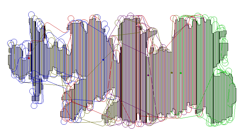
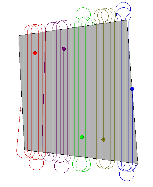
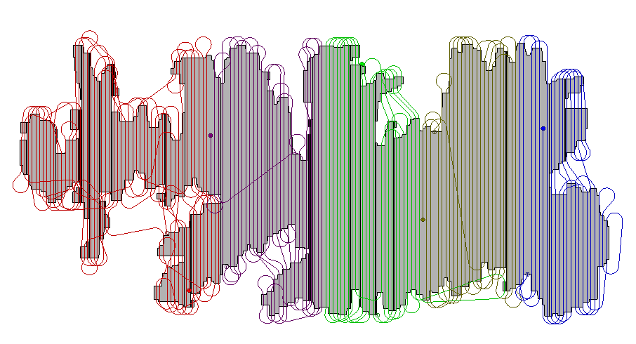
Figure 3: A simulation instance of DCRC (first row) and DCAC (second row) algorithms with 5 robots performing coverage over the area of interest indicated in gray, where the first column shows a small segment in the Lake Murray ($200\text{\times}200\text{\,}\mathrm{m}$); second column, Rural Quebec ($13\text{\times}10\text{\,}\mathrm{km}$); third column, the complete Lake Murray ($25\text{\times}25\text{\,}\mathrm{km}$).

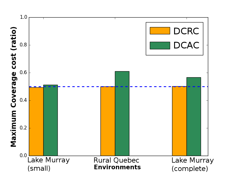
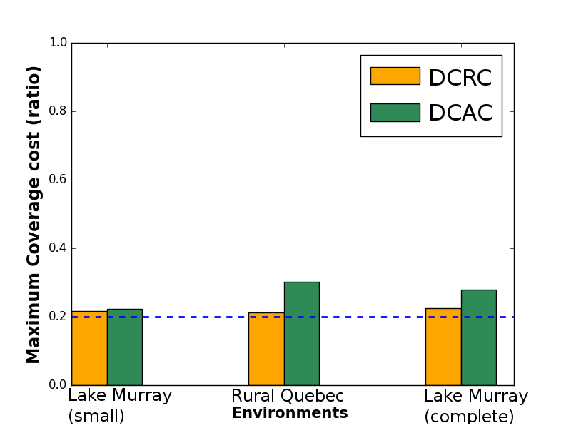
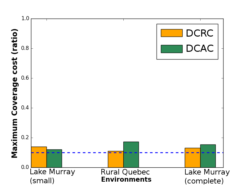
Figure 4: The comparison of actual maximum coverage cost and the ideal cost for three different environments for (a) $k=2$ (b) $k=5$ and (c) $k=10$ robots.

V-B Field trials

Given the better performance of DCRC, we validated the approach using DCRC with the ASVs, in a $200\text{\times}200\text{\,}\mathrm{m}$ area in Lake Murray, SC. The sensor footprint used had $4.5\text{\,}\mathrm{m}$ and the turning radius of the ASV is $5\text{\,}\mathrm{m}$. A path, in the form of a waypoint sequence, was generated with the ASVs starting just outside the area of interest. In the following, a description of the experiments performed and the results obtained.

The main objective of the field trials was to ensure that the assumptions hold also with real robots, so that the ASVs are able to follow the trajectories generated by the proposed algorithms.

V-B1 Single Robot Coverage baseline

Similar to the simulation experiments, the single robot coverage for Dubins Vehicles algorithm [8] is used here as a baseline for comparison with the multi-robot approach.

Figure 5 and Figure 5 present the ideal path and the path followed by the ASV, respectively, as recorded GPS points overlaid on Google Maps. The depth measurements were combined using a Gaussian Process (GP) mapping technique [33] to reconstruct the floor map of that part of the lake—see Figure 5.

V-B2 Multi-Robot Coverage Experiments

A variety of experiments were performed using teams of two or three robots in different areas of Lake Murray.

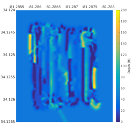
Figure 5: Multi-robot experiments at Lake Murray, SC, USA. 5 Ideal path produced for two robots. 5 Ideal path produced for three robots. 5 GPS track of the actual coverage path for two robots. 5 GPS track of the actual coverage path for three robots. 5 Depth map produced using a GP-based mapping using data from two robots. 5 Depth map produced using a GP-based mapping using data from three robots.

Figures 5 and 5 shows the ideal path for two and three ASVs as generated by DCRC; while Figures 5 and 5 shows the actual path followed by two and three robots, respectively. As can be seen qualitatively in Figures 5 and 5, the path followed by the ASVs are pretty much in line with the ideal path. The small deviations are due to GPS error, current, wind, and waves from other vessels. As such, the proposed methods can be applied for coverage with ASVs with Dubins constraints.

Note the ill-structured path of one of the robots (robot following the blue trajectory), result of a hardware failure and a hysteresis of its on-board PID controller. This illustrates the real world challenges with field trials: even if the boats are supposed to be identical, they are not, and they should undergo each of them an initial tuning phase of the different parameters of the boats. Such an issue opens interesting research directions on robust multi-robot coverage, including recovery mechanisms to adapt the algorithms to the new minimum turn radius and accounting for heterogeneity.

The resulting multi-robot coverage is also comparable to the single-robot coverage trajectory, where only small areas were left uncovered. Indeed, the bathymetric maps resulting from the single and multi-robot coverage are similar.

The maximum traveled distances per experiment with different number of robots are presented in Table I along with the ideal traveled distance. As in case of the simulation, the ideal path length is the size of the sub area if the tasks were exactly divided to equal parts.

TABLE I: The maximum distance traveled per robot and the cost of perfect division for multi-robot coverage experiments with the real ASVs.

Number of Robots	1	2	3
Max Distance	$6863\text{\,}\mathrm{m}$	$2905\text{\,}\mathrm{m}$	$3356\text{\,}\mathrm{m}$
Ideal Distance	$6863\text{\,}\mathrm{m}$	$3431.5\text{\,}\mathrm{m}$	$2287.7\text{\,}\mathrm{m}$

VI CONCLUSIONS

This paper presented a novel approach for multi-robot coverage utilizing multiple ASVs governed by Dubins vehicle kinematics. Both presented algorithms are extending our previous work on efficient multi-robot coverage with Dubins coverage algorithm.

The further clustering of the area ensures 100% utilization of robots. We show the validity and scalability of both approaches in simulation. The experiments show that both algorithms result in almost optimal solutions. Nevertheless, DCRC algorithm demonstrated slight advantage over DCAC algorithm in terms of coverage cost. As a result, our choice of algorithm was DCRC for performing field trials. The field trials were performed on a 200 $\textrm{km}^{2}$ region on Lake Murray, SC, USA. During the multi-robot coverage in a few instances, two vehicles came too close to each other.

We are currently investigating an automated arbitration mechanism following the rules of the sea [34] to avoid collisions. Furthermore, a camera system is being developed to provide situational awareness of the surroundings during operations. In general, the multi-robot coverage problem has several directions of interest, in particular taking into account the robustness of the proposed methods in real world.

References

- [1] H. Choset, “Coverage for robotics – a survey of recent results,” Ann. Math. Artif. Intel., vol. 31(1-4), pp. 113–126, 2001.
- [2] E. Galceran and M. Carreras, “A survey on coverage path planning for robotics,” Robot. Auton. Syst., vol. 61(12), pp. 1258 – 1276, 2013.
- [3] I. Rekleitis, A. New, E. S. Rankin, and H. Choset, “Efficient boustrophedon multi-robot coverage: an algorithmic approach,” Ann. Math. Artif. Intel., vol. 52(2-4), pp. 109–142, 2008.
- [4] A. Xu, C. Viriyasuthee, and I. Rekleitis, “Efficient complete coverage of a known arbitrary environment with applications to aerial operations,” Auton. Robot., vol. 36(4), pp. 365–381, 2014.
- [5] S. Manjanna, J. Hansen, A. Quattrini Li, I. Rekleitis, and G. Dudek, “Collaborative sampling using heterogeneous marine robots driven by visual cues,” in Proc. CRV, 2017, pp. 87–94.
- [6] L. E. Dubins, “On curves of minimal length with a constraint on average curvature, and with prescribed initial and terminal positions and tangents,” Am. J. Math., vol. 79, no. 3, pp. 497–516, 1957.
- [7] X. Yu and J. Y. Hung, “Coverage path planning based on a multiple sweep line decomposition,” in Proc. IEEE Industrial Electronics Society (IECON), 2015, pp. 004 052–004 058.
- [8] J. Lewis, W. Edwards, K. Benson, I. Rekleitis, and J. O’Kane, “Semi-boustrophedon coverage with a dubins vehicle,” in Proc. IROS, 2017, pp. 5630–5637.
- [9] N. Karapetyan, K. Benson, C. McKinney, P. Taslakian, and I. Rekleitis, “Efficient multi-robot coverage of a known environment,” in Proc. IROS, 2017, pp. 1846–1852.
- [10] P. Segui-Gasco, H.-S. Shin, A. Tsourdos, and V. J. Seguí, “Decentralised submodular multi-robot task allocation,” in Proc. IROS, 2015, pp. 2829–2834.
- [11] H. Choset, “Coverage of known spaces: The boustrophedon cellular decomposition,” Auton. Robot., vol. 9(3), pp. 247–253, 2000.
- [12] E. U. Acar and H. Choset, “Sensor-based Coverage of Unknown Environments: Incremental Construction of Morse Decompositions,” Int. J. Robot. Res., vol. 21(4), pp. 345–366, 2002.
- [13] Y. Gabriely and E. Rimon, “Spanning-tree based coverage of continuous areas by a mobile robot,” Ann. Math. Artif. Intel., vol. 31(1-4), pp. 77–98, 2001.
- [14] N. Hazon and G. Kaminka, “Redundancy, efficiency and robustness in multi-robot coverage,” in Proc. ICRA, 2005, pp. 735–741.
- [15] N. Agmon, H. Noam, G. A. Kaminka, and The MAVERICK Group, “The giving tree: constructing trees for efficient offline and online multi-robot coverage,” Ann. Math. Artif. Intel., vol. 52(2-4), pp. 143–168, 2008.
- [16] P. Fazli, A. Davoodi, P. Pasquier, and A. Mackworth, “Complete and robust cooperative robot area coverage with limited range,” in Proc. IROS, 2010, pp. 5577–5582.
- [17] A. Renzaglia, L. Doitsidis, S. A. Chatzichristofis, A. Martinelli, and E. B. Kosmatopoulos, “Distributed multi-robot coverage using micro aerial vehicles,” in Proc. Med. Control, 2013, pp. 963–968.
- [18] R. Mannadiar and I. Rekleitis, “Optimal coverage of a known arbitrary environment,” in Proc. ICRA, 2010, pp. 5525–5530.
- [19] J. Edmonds and E. L. Johnson, “Matching, Euler tours and the Chinese postman,” Math. Program., vol. 5, pp. 88–124, 1973.
- [20] K. Savla, F. Bullo, and E. Frazzoli, “The coverage problem for loitering dubins vehicles,” in Proc. CDC, 2007, pp. 1398–1403.
- [21] W. Huang, “Optimal line-sweep-based decompositions for coverage algorithms,” in Proc. ICRA, vol. 1, 2001, pp. 27–32.
- [22] Z. Yao, “Finding efficient robot path for the complete coverage of a known space,” in Proc. ICRA, 2006, pp. 3369–3374.
- [23] J. L. Ny, E. Feron, and E. Frazzoli, “On the dubins traveling salesman problem,” IEEE Trans. Automat. Contr., vol. 57, pp. 265–270, 2012.
- [24] K. Savla, E. Frazzoli, and F. Bullo, “On the point-to-point and traveling salesperson problems for dubins’ vehicle.” in Proc. ACC, 2005, pp. 786–791.
- [25] G. S. C. Avellar, G. A. S. Pereira, L. C. A. Pimenta, and P. Iscold, “Multi-UAV Routing for Area Coverage and Remote Sensing with Minimum Time,” Sensors, vol. 15(11), p. 27783, 2015.
- [26] P. Toth and D. Vigo, Eds., The Vehicle Routing Problem. Philadelphia, PA, USA: Society for Industrial and Applied Mathematics, 2001.
- [27] B. Xin, Y.-G. Zhu, Y.-L. Ding, and G.-Q. Gao, “Coordinated motion planning of multiple robots in multi-point dynamic aggregation task,” in Proc. ICCA, 2016, pp. 933–938.
- [28] I. A. Wagner, M. Lindenbaum, and A. M. Bruckstein, “Distributed covering by ant-robots using evaporating traces,” IEEE Transactions on Robotics and Automation, vol. 15(5), pp. 918–933, 1999.
- [29] A. Janani, L. Alboul, and J. Penders, “Multi-agent cooperative area coverage: Case study ploughing,” in Proc. AAMAS, 2016, pp. 1397–1398.
- [30] ——, Multi Robot Cooperative Area Coverage, Case Study: Spraying. Sheffield, UK Cham: Springer Int. Publishing, Jun. 2016, pp. 165–176.
- [31] G. N. Frederickson, M. S. Hecht, and C. E. Kim, “Approximation algorithms for some routing problems,” in Annual Symposium on Foundations of Computer Science (SFCS). IEEE Computer Society, 1976, pp. 216–227.
- [32] M. Quigley, K. Conley, B. P. Gerkey, J. Faust, T. Foote, J. Leibs, R. Wheeler, and A. Y. Ng, “ROS: an open-source Robot Operating System,” in ICRA Workshop on Open Source Software, 2009.
- [33] C. Rasmussen and C. Williams, Gaussian Processes for Machine Learning. MIT Press, 2006.
- [34] U.S. Department of Homeland Security, United States Coast Guard, “Navigation rules: International-inland,” https://www.navcen.uscg.gov/pdf/navrules/navrules.pdf, COMDTINST M16672.2D.