Minimum model for the electronic structure of
twisted bilayer graphene and related structures

Abstract

We introduce a minimum tight-binding model with only three parameters extracted from graphene and untwisted bilayer graphene. This model reproduces quantitatively the electronic structure of not only these two systems and bulk graphite near the Fermi level, but also that of twisted bilayer graphene including the value of the first magic angle, at which bands at $E_{F}$ flatten without overlap and two gaps open, one above and one below $E_{F}$. Our approach also predicts the second and third magic angle. The Hamiltonian is sufficiently transparent and flexible to be adopted to other twisted layered systems.

The electronic structure of graphite has been described quantitatively as early as 1947 by Wallace Wallace (1947) and found to be dominated by $p_{\perp}$ orbitals Slonczewski and Weiss (1958) near the Fermi level $E_{F}$. It is amazing how this system continues providing surprises in the behavior of charge carriers near $E_{F}$. In monolayer graphene (MLG), described quantitatively by a one-parameter Hamiltonian Castro Neto et al. (2009), backscattering of the massless fermions near the Dirac point $K$ in the corner of the hexagonal Brillouin zone (BZ) is suppressed due to the Klein paradox. In bilayer graphene (BLG) with the Bernal AB layer stacking, the inter-layer interaction turns the linear band dispersion at $K$ to a parabola and massless fermions in MLG to massive fermions in BLG and graphite. Most recently, correlated insulating Cao et al. (2018a) and unconventional superconducting Cao et al. (2018b) behavior have been reported in magic-angle twisted bilayer graphene (TBLG). Theoretical description of TBLG turns out to be challenging, since unit cells in the Moiré pattern of the bilayer become infinitely large for the general case of incommensurate structures. An elegant solution to this problem has been provided, treating the inter-layer interaction in a continuum model and handling the inter-layer matrix elements in reciprocal space Lopes dos Santos et al. (2007); Bistritzer and MacDonald (2011); Lopes dos Santos et al. (2012). Even though band flattening at $E_{F}$ and gap opening near $E_{F}$ have been predicted theoretically using many approaches Suárez Morell et al. (2010); Bistritzer and MacDonald (2011); Trambly de Laissardière et al. (2012); Moon and Koshino (2012); Lopes dos Santos et al. (2012); Jung et al. (2014); Cao et al. (2016); Fang and Kaxiras (2016); Nam and Koshino (2017); Kim et al. (2017), none has succeeded so far to reproduce the observed value of the (first) magic angle $\theta_{m,1}=1.1^{\circ}$ accompanied by a band flattening without band overlap at $E_{F}$, opening of band gaps both below and above the flat bands Cao et al. (2018a, b), and a sharp resistance increase at the charge neutrality point.

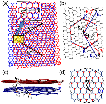
Figure 1: (Color online) Schematic structure of TBLG. (a) Moiré superlattice formed by placing layer 2 (red), twisted by $\theta$, on top of layer 1 (blue). The lattice vectors ${\bf{{a}_{1}}}$ and ${\bf{{a}_{2}}}$, also shown in the enlarged inset, span the Bravais lattice of layer 1. The primed quantities correspond to layer 2, and the superscript $(s)$ identifies the Moiré superlattice. (b) Large Brillouin zone of layer 1 (blue), spanned by $\bf{b_{1}}$ and $\bf{b_{2}}$, and of the twisted layer 2 (red), spanned by ${\bf{b^{\prime}_{1}}}$ and ${\bf{b^{\prime}_{2}}}$. The inequivalent Dirac points $K$ and $K^{\prime}$ are in the corners of the hexagonal unit cells of the individual layers. The small hexagonal Brillouin zones tiling the reciprocal space are spanned by ${\bf{b_{1}^{(s)}}}$ and ${\bf{b_{2}^{(s)}}}$. (c) Definition of interatomic distances in adjacent layers separated by $d_{0}$ in perspective side view. (d) Brillouin zones in the reciprocal lattice of layer 1.

Here we construct a minimum tight-binding Hamiltonian with only three parameters extracted from MLG and untwisted BLG. This Hamiltonian reproduces quantitatively the electronic structure of not only these two systems and bulk graphite near $E_{F}$, but also that of TBLG including the values of the magic angles $\theta_{m,1}$, $\theta_{m,2}$, and $\theta_{m,3}$. At $\theta_{m,1}$, bands at $E_{F}$ flatten without overlap, two gaps open, one above and one below $E_{F}$. The Hamiltonian is sufficiently transparent and flexible to be adopted to other twisted layered systems.

As mentioned above, none of the computational approaches used so far to describe TBLG and the role of the magic angle has succeeded in reproducing all aspects of the observed data Cao et al. (2018a, b). An elegant description of TBLG using the continuum model and treatment of the inter-layer hopping in Fourier space has been introduced in Ref. Lopes dos Santos et al. (2007), but did not find gaps in the electronic spectrum in the range of twist angles $\theta$ investigated. The follow-up paper by the same authors Lopes dos Santos et al. (2012) did find the magic angle $\theta_{m,1}{\approx}1.1^{\circ}$ and both band gaps. However, the band gap dependence on the twist angle disagrees with more recent experimental data Cao et al. (2018a), likely due to an inaccurate description of the inter-layer interaction Tang et al. (1996). The magic angle was first predicted in the theoretical Ref. Bistritzer and MacDonald (2011), which also used the continuum model and treated the inter-layer hopping in Fourier space using experimentally obtained parameters. The authors discussed the occurrence of a flat band at $\theta_{m,1}$, but did not discuss band gaps near $E_{F}$. A separate calculation using the same approach Bistritzer and MacDonald (2011) reproduced only one gap below $E_{F}$. No band gaps were found near $E_{F}$ in the follow-up study Jung et al. (2014) based completely on ab initio density functional theory (DFT). The continuum model and Fourier space treatment were abandoned in a detailed DFT study of Ref.Fang and Kaxiras (2016) applied to commensurate structures. The DFT results, obtained using maximally localized Wannier functions, were mapped onto a tight-binding Hamiltonian with 18 parameters, which was diagonalized directly in the large Moiré supercells. Even though this approach reproduces the band flattening at the magic angle, the authors reported only one band gap above $E_{F}$. A related approach to determine the electronic spectrum, which relies on the Hubbard model rather than DFT, has recently been proposed Koshino et al. (2018) as an extension of the initial tight-binding description of TBLG in terms of $V_{pp\pi}$ intra-layer and $V_{pp\sigma}$ inter-layer two-center hopping integrals Moon and Koshino (2012). Whereas the initial report Moon and Koshino (2012) found band gaps only for large twist angles beyond $\theta_{m,1}$, a follow-up study using the same approach Nam and Koshino (2017) reported crossing flat bands at the charge neutrality point, in contrast to the observed sharp resistance increase,Cao et al. (2018a) and claimed that band gap opening at $\theta_{m,1}$ is caused by lattice relaxation. The necessity to determine lattice relaxation to reproduce experimental observations is computationally extremely demanding Koshino et al. (2018) and thus limits the size of the Moiré supercells in the commensurate structure, making prediction of higher magic angles extremely difficult. All reported theoretical results suggest that the low-energy electronic structure of TBLG near $\theta_{m,1}$ is rather sensitive to the model description and the parameters.

We combined the most attractive aspects of the above theoretical approaches in a minimum model that is consistent with experimental data Cao et al. (2018a, b). The Hamiltonian we propose for any graphitic system consists of an intra-layer part $H_{\parallel}$ and an inter-layer part $H_{\perp}$. The description we chose combines simplicity and transparency with the benefits of previously used models while avoiding their different shortcomings. This Hamiltonian reads

$$H = H_{\parallel}+H_{\perp}$$ (1)

$$= -\sum_{{i{\neq}j}\atop{m}}\gamma_{ij}^{mm}(c^{+}_{m,i}c^{\,}_{m,j}+h.c.)$$

$$-\sum_{{i,j}\atop{m}}\gamma_{ij}^{m,m+1}(c^{+}_{m,i}c^{\,}_{m+1,j}+h.c.)\;.$$

Here, $c^{+}_{m,i}$ is the creation and $c^{\,}_{m,i}$ is the annihilation operator of a $p_{z}$ state at the atomic site $i$ in layer $m$, with $m=1$ or $2$ for BLG. $\gamma_{ij}^{mm}$ is the in-plane hopping integral between sites $i$ and $j$.

Typically, only nearest neighbor intra-layer hopping is considered in $H_{\parallel}$. $\gamma_{<ij>}^{mm}=V^{0}_{pp\pi}=3.09$ eV reproduces the Fermi velocity Castro Neto et al. (2009) $v_{F}{\approx}1{\times}10^{6}$ m/s in the graphene layer spanned by lattice vectors $\bf{a_{1}}$ and $\bf{a_{2}}$, shown in Fig. 1(a), with $|{\bf{a_{1}}}|=|{\bf{a_{2}}}|=a$. The corresponding reciprocal lattice vectors $\bf{b_{1}}$ and $\bf{b_{2}}$, defining the BZ of the layer, are shown in Fig. 1(b).

To describe the inter-layer interaction in $H_{\perp}$, we first considered an AB-stacked untwisted BLG, as illustrated in Fig. 1(c). We first consider two atoms atop each other in adjacent layers, at the positions $\bf{r_{1,i}}$ and $\bf{r_{2,i}}$, separated by the inter-layer distance $d_{0}$. The inter-layer hopping integral between these atoms is $t(0)=\gamma_{ii}^{1,2}=V^{0}_{pp\sigma}$. Next, we consider one of the atoms moving within the layer, so that the mutual distance vector, projected on one of the layers, becomes $|{\bf{r}}|=r>0$. For $r$ not very large, the dominant inter-layer hopping integral is still $V_{pp\sigma}$, scaled by the distance and corrected for the cosine of the tilting angle Moon and Koshino (2012). It is isotropic and can be written as

$$t(r)=V^{0}_{pp\sigma}e^{-(\sqrt{r^{2}+d_{0}^{2}}-d_{0})/\lambda}\frac{d_{0}^{2}}{r^{2}+d_{0}^{2}}\,,$$ (2)

where $\lambda$ modulates the cutoff of $t(r)$ at large distances. This expression allows a flexible description of the inter-layer interaction in regions of local AA and AB stacking as well as in-between.

Precise observations for AB-stacked untwisted BLG provided accurate values $a=2.46$ Å, $d_{0}=3.35$ Å and $V^{0}_{pp\sigma}=0.39$ eV$=\gamma_{1}$ in standard graphite notation. Using ${\lambda}=0.27$ Å, we could furthermore reproduce the well-established band structure of AA- and AB-stacked BLG. This value of ${\lambda}$ also yielded $\gamma_{3}=\gamma_{4}=0.11$ eV for neighbors in adjacent layers with $r=a/\sqrt{3}$ in very good agreement with experimental data Lambert and Côté (2013); Yankowitz et al. (2014); Knothe and Jolicoeur (2016). All parameters needed to reproduce the electronic structure of MLG, BLG, graphite and TBLG are listed in Table 1. As we will show, Hamiltonian (1) also reproduces the magic angle $\theta_{m,1}{\approx}1.1^{\circ}$, band flattening without band overlap at $E_{F}$, opening of two gaps, one below and one above $E_{F}$, and band gap reduction for twist angles deviating from $\theta_{m,1}$.

Table 1: Band-structure parameters of graphitic systems.

Quantity	$a$		$d_{0}$		$V^{0}_{pp\pi}$		$V^{0}_{pp\sigma}$		$\lambda$
Value	$2.46$ Å		3.35 Å		3.09 eV		0.39 eV		$0.27$ Å

In the following, we will describe a TBLG initially formed as an AA stacked BLG, where the top layer 2 has been twisted counterclockwise by the angle $\theta$ with respect to the bottom layer 1, as seen in top view in Fig. 1(a). The honeycomb lattice of a graphene layer consists of a triangular Bravais lattice with a two-atom basis. The vectors spanning the Bravais lattice of the bottom layer 1 are ${\bf{{a}_{1}}}=a(\sqrt{3}/2,-1/2)$ and ${\bf{{a}_{2}}}=a(\sqrt{3}/2,1/2)$ in Cartesian coordinates. The positions of the two basis atoms A and B in the unit cell, which form the sublattices A and B, are ${\bf{{\tau}_{A}}}=({\bf{{a}_{1}}}+{\bf{{a}_{2}}})/3$ and ${\bf{{\tau}_{B}}}=2({\bf{{a}_{1}}}+{\bf{{a}_{2}}})/3$. The Bravais lattice vectors spanning the twisted upper layer 2 are ${\bf{{a^{\prime}}_{1}}}$ and ${\bf{{a^{\prime}}_{2}}}$ and the basis vectors spanning the sublattices are ${\bf{{\tau}_{\alpha}^{\prime}}}$. The reciprocal lattice of the bottom layer 1, spanned by ${\bf{b}_{1}}$ and ${\bf{b}_{2}}$, is shown in Fig. 1(d).

For commensurate TBLG lattices, we can use the index $(M,N)$ to define the twist angle $\theta$ and the Moiré supercell Fang and Kaxiras (2016). Incommensurate lattices can still be approximated by a commensurate lattice with a specific index $(M^{\prime},N^{\prime})$ and ${\theta}^{\prime}{\approx}\theta$, albeit with possibly very large supercells. The reciprocal lattice of the $(N+1,N)$ TBLG with a small twist angle, shown in Fig. 1(b), is spanned by the vectors ${\bf{b_{1}^{(s)}}}={\bf{b}_{2}}-{\bf{b^{\prime}}_{2}}$, and ${\bf{b_{2}^{(s)}}}=({\bf{b^{\prime}}_{1}}+{\bf{b^{\prime}}_{2}})-({\bf{b}_{1}}+{\bf{b}_{2}})$, where ${\bf{b}_{i}}$ and ${\bf{b^{\prime}}_{i}}$ with $i=1,2$ are reciprocal lattice vectors of the bottom and the top layer, respectively.

In the following, we will focus on a TBLG lattice with small twist angles near the observed magic angle $\theta_{m,1}{\approx}1.1^{\circ}$. Whether commensurate or incommensurate, such a lattice can be described or approximated by a commensurate lattice with a large Moiré supercell and the electronic structure can be obtained to a good accuracy using the continuum method. In this approach, the low-energy wavefunctions can be expanded in the Bloch basis of the bottom layer 1 and the twisted top layer 2 near the Dirac point, which are defined as

$$|\psi_{1,\alpha}({\bf{k}})\rangle = \frac{1}{\sqrt{N}}\sum_{{\bf{R}}}e^{i{\bf{k}}{\cdot}({\bf{R}}+{\bf{\tau}_{\alpha}})}|{\bf{R}}+{\bf{\tau}_{\alpha}}\rangle,$$

$$|\psi_{2,\alpha}({\bf{k}})\rangle = \frac{1}{\sqrt{N}}\sum_{{\bf{R}}^{\prime}}e^{i{\bf{k}}{\cdot}({\bf{R^{\prime}}}+{\bf{\tau}^{\prime}_{\alpha}})}|{\bf{R^{\prime}}}+{\bf{\tau}^{\prime}_{\alpha}}\rangle\,.$$ (3)

Here, the index $\alpha$ denotes the $A$ or $B$ sublattice, and the Wannier function $|{\bf{R}}+{\bf{\tau}_{\alpha}}\rangle$ is the $p_{z}$ orbital at that site. To discuss the value range of $\bf{k}$, we refer to Fig. 1(b) depicting the large hexagonal Brillouin zone of layer 1 spanned by $\bf{b_{1}}$ and $\bf{b_{2}}$ and the counterparts for the twisted layer 2, and the smaller Brillouin zones of the Moiré superlattice, spanned by ${\bf{b_{1}^{(s)}}}$ and ${\bf{b_{2}^{(s)}}}$. In the vicinity of the Dirac point $K$ of layer 1 and its counterpart in twisted layer 2, we can express ${\bf{k}}={\bf{k}}^{(s)}+{\bf{k}}_{0}+{\bf{G}^{(s)}}$, where ${\bf{k}}^{(s)}$ is a $\bf{k}$-point in the supercell BZ in the center of the BZ of the monolayers and ${\bf{k}}_{0}$ is the center of one of the supercell BZs containing $K$ of layer 1 in their corners. ${\bf{G}^{(s)}}$ is a reciprocal lattice vector of the superlattice, given by ${\bf{G}^{(s)}}=n_{1}~{}{\bf{b_{1}^{(s)}}}+n_{2}~{}{\bf{b_{2}^{(s)}}}$ with small integers $n_{1}$ and $n_{2}$ typically in the range $-4{\leq}n_{i}{\leq}+4$.

Defining ${\bf{k_{1}}}={\bf{k}}^{(s)}+{\bf{k}}_{0}+{\bf{G_{1}}^{(s)}}$ and ${\bf{k_{2}}}={\bf{k}}^{(s)}+{\bf{k}}_{0}+{\bf{G_{2}}^{(s)}}$, the intra-layer Hamilton matrix elements are given in the Bloch basis by

$$\langle\psi_{m,\alpha}({\bf{k_{1}}})|H|\psi_{m,\beta}({\bf{k_{2}}})\rangle=H_{m,\alpha\beta}({\bf{k_{1}}})\delta_{{\bf{G_{1}}^{(s)}},{\bf{G_{2}}^{(s)}}}\,,$$ (4)

with $m=1,2$ defining the layer and $\alpha$ the sublattice. The on-site energy for both layers is set to be zero, so the diagonal matrix elements of the Hamiltonian are $H_{m,\alpha\alpha}({\bf{k}})=0$. For the two layers 1 and 2, the off-diagonal matrix elements of the Hamiltonian are given by

$$H_{1,AB}({\bf{k}})=-V^{0}_{pp\pi}\sum_{j=1}^{3}e^{i{\bf{k}}{\cdot}{\bf{\rho_{j}}}}\,,$$

$$H_{2,AB}({\bf{k}})=-V^{0}_{pp\pi}\sum_{j=1}^{3}e^{i{\bf{k}}{\cdot}{\bf{{\rho}^{\prime}_{j}}}}\,,$$ (5)

where $V^{0}_{pp\pi}$ is the intra-layer nearest-neighbor hopping term. ${\bf{\rho_{j}}}$ are the vectors connecting sublattice A sites to their three nearest neighbors in sublattice B in layer 1. ${\bf{{\rho}^{\prime}_{j}}}$ are the corresponding nearest-neighbor vectors in the twisted layer 2. The Hamiltonian is Hermitian, so $H_{m,BA}({\bf{k}})=H_{m,AB}^{*}({\bf{k}})$ for $m=1,2$.

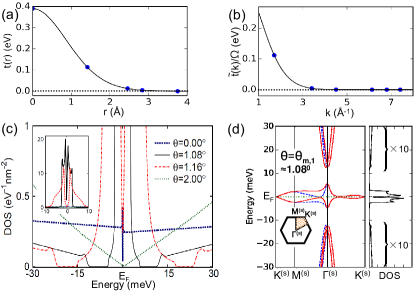
Figure 2: (Color online) (a) The inter-layer hopping integral $t(r)$, defined in Eq. (2), and (b) its Fourier transform $\tilde{t}(k)$. The filled circles in (a) represent possible $r$ values in AB-stacked BLG. (c) Electronic density of states (DOS) of TBLG near $E_{F}$ for different twist angles $\theta$. The DOS for $\theta=0$ represents an untwisted BLG. (d) The electronic band structure of TBLG along high-symmetry lines of the Moiré superlattice (left) and the corresponding DOS (right) for $\theta$ near the (first) magic angle $\theta_{m,1}{\approx}1.08^{\circ}$. The red (dashed blue) lines represent bands with the valley index $K$ ($K^{\prime}$) defined in Fig. 1(d). The DOS below and above $E_{F}$ is multiplied by $10$. The BZ of the superlattice is shown as an inset in the band structure.

To describe the inter-layer coupling in an effective, approximate way, we fist consider the atomic distribution in a 2D graphene layer to be continuous uniform. In that case, the 2D Fourier transform of $t({\bf{r}})$ is given by

$$\tilde{t}({\bf{k}})=\int e^{-i{\bf{k}}{\cdot}{\bf{r}}}t({\bf{r}})d^{2}r\,.$$ (6)

Since $t({\bf{r}})$ is isotropic, Eq. (6) can be transformed to a 1D integral

$$\tilde{t}(k)=2\pi\int_{0}^{\infty}rt(r)J_{0}(kr)dr\,,$$ (7)

where $J_{0}$ is a Bessel function and the Fourier transform is also isotropic in the reciprocal space. The radial dependence of the inter-layer hopping integral $t(r)$ is shown in Fig. 2(a) and it Fourier transform $\tilde{t}(k)$ is shown in Fig. 2(b).

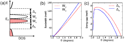
Figure 3: (Color online) Electronic structure of TBLG near the magic angle $\theta_{m,1}{\approx}1.1^{\circ}$. (a) Schematic electronic structure near the charge neutrality point. The flat band splits into two narrow valence bands of width $W_{v}$ and two narrow conduction bands of width $W_{c}$. A band gap of width $\Delta_{h}$ opens on the hole side below $E_{F}$ and a gap of width $\Delta_{e}$ opens on the electron side above $E_{F}$. (b) $W_{v}$ and $W_{c}$ as a function of the twist angle $\theta$. (c) $\Delta_{h}$ and $\Delta_{e}$ as a function of $\theta$.

For TBLG with a small twist angle, where the continuum model is justified, the inter-layer Hamilton matrix elements can be evaluated and expanded in the reciprocal space as Bistritzer and MacDonald (2011)

$$\langle\psi_{1,\alpha}({\bf{k_{1}}})|H|\psi_{2,\beta}({\bf{k_{2}}})\rangle=$$

$$\sum_{{\bf{G}}}\frac{\tilde{t}({\bf{k_{1}}}+{\bf{G}})}{\Omega}e^{i({\bf{G}}{\cdot}{\bf{\tau}_{\alpha}}-{\bf{G}}{\cdot}{\bf{\tau}_{\beta}})}\delta_{{\bf{k_{2}}}-{\bf{k_{1}}},{\bf{G}}-{\bf{G^{\prime}}}}\,.$$ (8)

Here, ${\bf{G}}$ are reciprocal lattice vectors of the untwisted graphene layer 1, ${\bf{G^{\prime}}}$ are the corresponding vectors of the twisted layer 2, and $\Omega$ is the area of the graphene unit cell. ${\bf{k_{1}}}$ and ${\bf{k_{2}}}$ have been defined earlier for use in the intra-layer Hamilton matrix elements in Eq. (4).

In the expansion over the reciprocal lattice of layer 1, we found that 27 ${\bf{G}}$-vectors, indicated by orange circles in Fig. 1(d), are necessary to reach convergence of the electronic structure due to the larger extent of the Fourier-transformed inter-layer hopping integral $\tilde{t}(k)$ associated with our small value of $\lambda$. In previous studies Lopes dos Santos et al. (2007); Bistritzer and MacDonald (2011), only 3 small ${\bf{G}}$-vectors have been used for the expansion in Eq. (8). Even in this restricted expansion, the authors probed the relevant part of reciprocal space near the Dirac point ${\bf{K}}$, since $|{\bf{K}}+{\bf{G}}|$ is close to $|{\bf{K}}|$. In the expansion of TBLG wavefunctions, we use a $9{\times}9$ grid of ${\bf{G}^{(s)}}$-vectors for each value of ${\bf{k}}^{(s)}$.

Recent observations Cao et al. (2018a, b) suggest that the (first) magic angle in TBLG, accompanied by a band flattening and a sharp resistance increase at the charge neutrality point, caused by vanishing band overlap, occurs at $\theta_{m,1}{\approx}1.08^{\circ}$. Even though the magic angle structure is likely incommensurate, nearby twist angle values may be obtained considering commensurate TBLGs with index $(N+1,N)$. Since the BZ collapses to zero in incommensurate structures, only the DOS and not the band structure can be provided. The DOS of TBLG with $\theta$ in the range from $0^{\circ}{-}2^{\circ}$, with emphasis on the first magic angle $\theta_{m,1}$, is shown in Fig. 2(c) and as movie in the Supporting Material TBL . Also presented in the Supporting Material TBL is the calculated DOS near the second magic angle $\theta_{m,2}{\approx}0.47^{\circ}$ and the third magic angle $\theta_{m,3}{\approx}0.28^{\circ}$. These values agree well with previously reported values Bistritzer and MacDonald (2011) $\theta_{m,2}{\approx}0.50^{\circ}$ and $\theta_{m,3}{\approx}0.35^{\circ}$. The incommensurate structure with the magic angle $\theta_{m,1}$ can be approximated by a TBLG with index $(31,30)$ and twist angle $\theta=1.08455^{\circ}$. For this commensurate structure, we present both the band structure $E(k)$ and the DOS in Fig. 2(d). We notice that at $\theta_{m,1}$, the flat band splits into valence and conduction sub-bands originating from $K$ and $K^{\prime}$ valleys shown in Fig. 1(b). These bands do not overlap at $\theta_{m,1}$, providing an explanation for the sharp resistance increase at the charge neutrality point.

The TBLG DOS near $\theta_{m,1}$ is shown schematically in Fig. 3(a). Below $E_{F}$, two flat valence bands of width $W_{v}$ are separated by a hole gap of width $\Delta_{h}$ from lower-lying occupied states. Above $E_{F}$, two flat conduction bands of width $W_{c}$ are separated by an electron gap of width $\Delta_{e}$ from higher occupied states. As seen in Figs. 3(b) and 3(c), the minimum values $W_{v}$ and $W_{c}$ with the bands not overlapping and no gaps above or below $E_{F}$ occur near $\theta_{m,1}$. According to Fig. 3(c), even a small increase of $\theta$ beyond $\theta_{m,1}$ opens gaps above and below the flat band. Even though $\Delta_{h}>\Delta_{e}$ in general, both gaps decrease in size with increasing value of $\theta$ and eventually close for $\theta{\gtrsim}1.7^{\circ}$. As seen in Fig. 2(c), the DOS of TBLG with $\theta=2^{\circ}$ shows no indication of any band gap or a flat band.

In our minimum description, all parameters listed in Table 1 have well-established values based on experimental observation. The only variable that required a judicious choice was that of the decay length $\lambda$. At $\theta_{m,1}$, the minimum values of $W_{v}$ and $W_{c}$ and thus the minimum width of the flat band $W_{fb}{\approx}1.9$ meV was obtained using $\lambda=0.21$ Å. In this case, overlap of the narrow valence and conduction bands along the $G^{(s)}-M^{(s)}$ direction yielded a rather large DOS at $E_{F}$, which is inconsistent with the observed high resistance at the neutrality point. We found $W_{fb}$ to increase for both $\lambda<0.21$ Å and $\lambda>0.21$ Å. The narrowest flat band with $W_{fb}{\approx}4.7$ meV and no overlap between the flat valence and conduction bands occurred for $\lambda=0.27$ Å. This value has been used throughout our study.

In conclusion, we introduced a minimum tight-binding Hamiltonian with only three parameters extracted from graphene and untwisted bilayer graphene. We found that this Hamiltonian reproduces quantitatively the electronic structure of not only these two systems and bulk graphite near the Fermi level, but also that of twisted bilayer graphene including the value of the first magic angle, at which bands at $E_{F}$ flatten without overlap and two gaps open, one above and one below $E_{F}$. Our approach also predicts the second and third magic angle. The Hamiltonian is sufficiently transparent and flexible to be adopted to other twisted layered systems.