Modified Gravity and Inflaton Assisted Dynamical Generation of Charge Confinement and Electroweak Symmetry Breaking in Cosmology

Abstract

We describe a new type of gravity-matter models where modified $f(R)=R+R^{2}$ gravity couples non-canonically to a scalar “inflaton”, to the bosonic sector of the electroweak particle model and to a special nonlinear gauge field with a square-root of the standard Maxwell/Yang-Mills kinetic term simulating QCD confining dynamics. Our construction is based on the powerful formalism of non-Riemannian space-time volume-forms – alternative metric-independent volume elements defined in terms of auxiliary antisymmetric tensor gauge fields. Our model provides a unified Lagrangian action principle description of: (i) the evolution of both “early” and “late” universe by the “inflaton” scalar field; (ii) gravity-inflaton-assisted dynamical generation of Higgs spontaneous breakdown of electroweak gauge symmetry in the “late” universe, as well as dynamical suppression of electroweak breakdown in the “early” universe; (iii) gravity-inflaton-assisted dynamical generation of QCD-like confinement in the “late” universe and suppression of confinement in the “early” universe due to the special interplay with the dynamics of the QCD-simulating nonlinear gauge field.

1 1. Introduction

One of the principal tasks in cosmology is the establishment from first principles, i.e., from Lagrangian action principle, of consistent mechanisms driving the appearance, respectively the suppression, of confinement and electroweak spontaneous symmetry breaking during the various stages in the evolution of the universe [1]-[7].

In the present note we will discuss in some detail the main interesting properties of a new type of non-canonical extended gravity-matter model, in particular, its implications for cosmology. Namely we will consider modified $f(R)=R+R^{2}$ gravity coupled in a non-standard way to a scalar “inflaton” field, to the bosonic fields of the standard electroweak particle model, as well as to a special kind of a nonlinear (Abelian or non-Abelian) gauge field with a square-root of the standard Maxwell/Yang-Mills kinetic term which simulates QCD confining dynamics. In this way our model will represent qualitatively extended gravity coupled to the whole (bosonic part of the) standard model of elementary particle physics.

The first essential non-standard feature of the model under consideration is its construction in terms of non-Riemannian spacetime volume-forms (alternative metric-independent generally covariant volume elements) defined in terms of auxiliary antisymmetric tensor gauge fields of maximal rank (see Refs.[8, 9] for a consistent geometrical formulation, which is an extension of the originally proposed method [10, 11]). The latter volume-form gauge fields were shown to be almost pure-gauge – apart from few arbitrary integration constants they do not produce additional propagating field-theoretic degrees of freedom (see Appendices A of Refs.[9, 12] and Section 2 below). Yet the non-Riemannian spacetime volume-forms trigger a series of important physical features unavailable in ordinary gravity-matter models with the standard Riemannian volume element (given by the square-root of the determinant of the Riemannian metric):

(i) The “inflaton” $\varphi$ develops a remarkable effective scalar potential in the Einstein frame possessing an infinitely large flat region for large negative $\varphi$ describing the “early” universe evolution;

(ii) In the absence of the $SU(2)\times U(1)$ iso-doublet scalar field, the “inflaton” effective potential has another infinitely large flat region for large positive $\varphi$ at much lower energy scale describing the “late” post-inflationary (dark energy dominated) universe;

(iii) Inclusion of the $SU(2)\times U(1)$ iso-doublet scalar field $\sigma$ – without the usual tachyonic mass and quartic self-interaction term – introduces a drastic change in the total effective scalar potential in the post-inflationary universe: the effective potential as a function of $\sigma$ dynamically acquires exactly the electroweak Higgs-type spontaneous symmetry breaking form. The latter is an explicit realization of Bekenstein’s idea [13] for a gravity-assisted dynamical electroweak spontaneous symmetry breaking.

(iv) Further important features arise upon introducing a coupling to an additional strongly nonlinear gauge field whose Lagrangian contains a square-root of the standard Maxwell/Yang-Mills kinetic term. The latter is known to describe charge confinement in flat spacetime [14] as well as in curved spacetime for static spherically symmetric field configurations (Appendix B in Ref.[9]; see also Eq.(26) below). This is a simple implementation of ‘t Hooft’s idea [15] about confinement being produced due to the presence in the energy density of electrostatic field configurations of a term linear w.r.t. electric displacement field in the infrared region (arising presumably as an appropriate infrared counterterm). Therefore, the addition of the “square-root” nonlinear gauge field will simulate the strong interactions QCD-like dynamics.

Let us particularly emphasize that the specific form of the action (Eq.(18) below) with the several non-Riemannian volume elements describing our model is uniquely determined by the requirement of global Weyl-scale symmetry (Eq.(27) below) which becomes spontaneously broken upon transferring to the physical Einstein frame.

As a result, in the Einstein frame we achieve:

(a) Bekenstein-inspired gravity-inflaton-assisted dynamical generation of Higgs-type electroweak spontaneous symmetry breaking in the “late” universe, while there is no electroweak breaking in the “early” universe;

(b) Simultaneously we obtain gravity-inflaton-assisted dynamical generation of charge confinement in the “late” universe as well as gravity-suppression of confinement, i.e., deconfinement in the “early” universe.

In Section 2 we briefly review the main properties of the non-Riemannian volume-forms on spacetime manifolds, including elucidating the (almost) pure gauge nature of the associated antisymmetric tensor gauge fields of maximal rank. In Section 3 we first provide the formulation of our non-canonical $f(R)$-gravity model coupled to the (bosonic part of the) standard model of elementary particles in terms of several different non-Riemannian spacetime volume-forms. Next we describe the construction of the corresponding physical Einstein-frame action. Section 4 discusses the main interesting implications for cosmology of the present model. Section 5 contains some conclusions and outlook.

2 2. Non-Riemannian Volume-Forms in Gravitational Theories

2.0.1 2.1 Non-Riemannian Volume-Forms - General Properties

Volume-forms (generally-covariant integration measures) in integrals over manifolds are given by nonsingular maximal rank differential forms $\omega$:

$$\int_{{\mathcal{M}}}\omega\bigl{(}\ldots\bigr{)}=\int_{{\mathcal{M}}}dx^{D}\,\Omega\bigl{(}\ldots\bigr{)}\;\;,\;\;\omega=\frac{1}{D!}\omega_{\mu_{1}\ldots\mu_{D}}dx^{\mu_{1}}\wedge\ldots\wedge dx^{\mu_{D}}\;,$$ (1)

$$\omega_{\mu_{1}\ldots\mu_{D}}=-\varepsilon_{\mu_{1}\ldots\mu_{D}}\Omega\;\;,\;\;dx^{\mu_{1}}\wedge\ldots\wedge dx^{\mu_{D}}=\varepsilon^{\mu_{1}\ldots\mu_{D}}\,dx^{D}\;,$$ (2)

(our conventions for the alternating symbols $\varepsilon^{\mu_{1},\ldots,\mu_{D}}$ and $\varepsilon_{\mu_{1},\ldots,\mu_{D}}$ are: $\varepsilon^{01\ldots D-1}=1$ and $\varepsilon_{01\ldots D-1}=-1$). The volume element (integration measure density) $\Omega$ transforms as scalar density under general coordinate reparametrizations.

In standard generally-covariant theories (with action $S=\int d^{D}\!x\sqrt{-g}{\mathcal{L}}$) the Riemannian spacetime volume-form is defined through the “D-bein” (frame-bundle) canonical one-forms $e^{A}=e^{A}_{\mu}dx^{\mu}$ ($A=0,\ldots,D-1$):

$$\omega=e^{0}\wedge\ldots\wedge e^{D-1}=\det\|e^{A}_{\mu}\|\,dx^{\mu_{1}}\wedge\ldots\wedge dx^{\mu_{D}}\quad\longrightarrow\quad\Omega=\det\|e^{A}_{\mu}\|\,d^{D}x=\sqrt{-\det\|g_{\mu\nu}\|}\,d^{D}x\;.$$ (3)

There is no a priori any obstacle to employ instead of $\sqrt{-g}$ another alternative non-Riemannian volume element as in (1)-(2) given by a non-singular exact $D$-form $\omega=dB$ where:

$$B=\frac{1}{(D-1)!}B_{\mu_{1}\ldots\mu_{D-1}}dx^{\mu_{1}}\wedge\ldots\wedge dx^{\mu_{-1}}\;,$$ (4)

so that the non-Riemannian volume element reads:

$$\Omega\equiv\Phi(B)=\frac{1}{(D-1)!}\varepsilon^{\mu_{1}\ldots\mu_{D}}\,\partial_{\mu_{1}}B_{\mu_{2}\ldots\mu_{D}}\;.$$ (5)

Here $B_{\mu_{1}\ldots\mu_{D-1}}$ is an auxiliary rank $(D-1)$ antisymmetric tensor gauge field. $\Phi(B)$, which is in fact the density of the dual of the rank $D$ field strength $F_{\mu_{1}\ldots\mu_{D}}=\frac{1}{(D-1)!}\partial_{[\mu_{1}}B_{\mu_{2}\ldots\mu_{D}]}=-\varepsilon_{\mu_{1}\ldots\mu_{D}}\Phi(B)$, similarly transforms as scalar density under general coordinate reparametrizations.

The presence of non-Riemannian volume element $\Phi(B)$ in a gravity-matter action $S=\int d^{D}\!x\Phi(B){\mathcal{L}}+\ldots$ does not change the number of field-theoretic degrees of freedom – the latter remains the same as with the standard Riemannian measure $\sqrt{-g}$.

In fact, as we will demonstrate in the next Subsection 2.2, the canonical Hamiltonian analysis reveals that the auxiliary gauge field $B_{\mu_{1}\ldots\mu_{D-1}}$ is (almost) pure-gauge! This is because the total Lagrangian is only linear w.r.t. $B$-velocities, so it leads to Hamiltonian constraints a’la Dirac. The only remnant of $B_{\mu_{1}\ldots\mu_{D-1}}$ is a discrete degree of freedom which appears as integration constant $M$ in the equations of motion w.r.t. $B_{\mu_{1}\ldots\mu_{D-1}}$ (see subsect. 3.2 below). $M$ is in fact a conserved Dirac constrained canonical momentum conjugated to the “magnetic” $B$-component $\frac{1}{(D-1)!}\varepsilon^{i_{1}\ldots i_{D-1}}B_{i_{1}\ldots i_{D-1}}$.

2.0.2 2.2 Canonical Hamiltonian Treatment of Gravity-Matter Theories with Non-Riemannian Volume-Forms

Here we provide a brief discussion of the application of the canonical Hamiltonian formalism to a general gravity-matter model involving several non-Riemannian spacetime volume elements of the type (18) discussed below (see also Appendices A in Refs.[9, 12]):

$$S=\int d^{4}x\Phi_{1}(A){\widetilde{L}}^{(1)}(u,\stackrel{{\scriptstyle.}}{{u}})+\int\Phi_{2}(B)\left[{\widetilde{L}}^{(2)}(u,\stackrel{{\scriptstyle.}}{{u}})+\frac{\Phi_{4}(H)}{\sqrt{-g}}\right]\;,$$ (6)

$$\Phi_{1}(A)=\frac{1}{3!}\varepsilon^{\mu\nu\kappa\lambda}\partial_{\mu}A_{\nu\kappa\lambda}\quad,\quad\Phi_{2}(B)=\frac{1}{3!}\varepsilon^{\mu\nu\kappa\lambda}\partial_{\mu}B_{\nu\kappa\lambda}\quad,\quad\Phi_{4}(H)=\frac{1}{3!}\varepsilon^{\mu\nu\kappa\lambda}\partial_{\mu}H_{\nu\kappa\lambda}\;,$$ (7)

where the Lagrangians ${\widetilde{L}}^{(1,2)}(u,\stackrel{{\scriptstyle.}}{{u}})$ include both matter and scalar curvature terms, and where $(u,\stackrel{{\scriptstyle.}}{{u}})$ collectively denote the set of the basic gravity-matter canonical variables $(u)=\bigl{(}g_{\mu\nu},\mathrm{matter}\bigr{)}$ and their respective velocities. In (6) $\Phi_{4}(H)$ is the density dual of the gauge-field strength of an additional auxiliary gauge field $H_{\mu\nu\lambda}$ necessary for the consistency of the model.

For the present purpose it is sufficient to concentrate only on the canonical Hamiltonian structure related to the auxiliary maximal rank antisymmetric tensor gauge fields $A_{\mu\nu\lambda},B_{\mu\nu\lambda},H_{\mu\nu\lambda}$ and their respective conjugate momenta.

For convenience we introduce the following short-hand notations for the dual field-strengths (7) of the auxiliary 3-index antisymmetric gauge fields (the dot indicating time-derivative):

$$\Phi_{1}(A)=\stackrel{{\scriptstyle.}}{{A}}+\partial_{i}A^{i}\quad,\quad A=\frac{1}{3!}\varepsilon^{ijk}A_{ijk}\;\;,\;\;A^{i}=-\frac{1}{2}\varepsilon^{ijk}A_{0jk}\;,$$ (8)

$$\Phi_{2}(B)=\stackrel{{\scriptstyle.}}{{B}}+\partial_{i}B^{i}\quad,\quad B=\frac{1}{3!}\varepsilon^{ijk}B_{ijk}\;\;,\;\;B^{i}=-\frac{1}{2}\varepsilon^{ijk}B_{0jk}\;,$$ (9)

$$\Phi_{4}(H)=\stackrel{{\scriptstyle.}}{{H}}+\partial_{i}H^{i}\quad,\quad H=\frac{1}{3!}\varepsilon^{ijk}H_{ijk}\;\;,\;\;H^{i}=-\frac{1}{2}\varepsilon^{ijk}H_{0jk}\;,$$ (10)

For the pertinent canonical momenta conjugated to (8)-(10) we have:

$$\pi_{A}={\widetilde{L}}^{(1)}(u,\stackrel{{\scriptstyle.}}{{u}})\quad,\quad\pi_{B}={\widetilde{L}}^{(2)}(u,\stackrel{{\scriptstyle.}}{{u}})+\frac{1}{\sqrt{-g}}(\stackrel{{\scriptstyle.}}{{H}}+\partial_{i}H^{i})\quad,\quad\pi_{H}=\frac{1}{\sqrt{-g}}(\stackrel{{\scriptstyle.}}{{B}}+\partial_{i}B^{i})\;,$$ (11)

and:

$$\pi_{A^{i}}=0\quad,\quad\pi_{B^{i}}=0\quad,\quad\pi_{H^{i}}=0\;.$$ (12)

The latter imply that $A^{i},B^{i},H^{i}$ will in fact appear as Lagrange multipliers for certain first-class Hamiltonian constraints (see Eqs.(16)-(17) below). For the canonical momenta conjugated to the basic gravity-matter canonical variables we have (using last relation (11)):

$$p_{u}=(\stackrel{{\scriptstyle.}}{{A}}+\partial_{i}A^{i})\frac{\partial}{\partial\stackrel{{\scriptstyle.}}{{u}}}{\widetilde{L}}^{(1)}(u,\stackrel{{\scriptstyle.}}{{u}})+\pi_{H}\sqrt{-g}\frac{\partial}{\partial\stackrel{{\scriptstyle.}}{{u}}}{\widetilde{L}}^{(2)}(u,\stackrel{{\scriptstyle.}}{{u}})\;.$$ (13)

Now, relations (11) and (13) allow us to obtain the velocities $\stackrel{{\scriptstyle.}}{{u}},\,\stackrel{{\scriptstyle.}}{{A}},\,\stackrel{{\scriptstyle.}}{{B}},\,\stackrel{{\scriptstyle.}}{{H}}$ as functions of the canonically conjugate momenta $\stackrel{{\scriptstyle.}}{{u}}=\stackrel{{\scriptstyle.}}{{u}}(u,p_{u},\pi_{A},\pi_{B},\pi_{H})$ etc. (modulo some Dirac constraints among the basic gravity-matter variables due to general coordinate and gauge invariances). Taking into account (11)-(12) (and the short-hand notations (8)-(10)) the canonical Hamiltonian corresponding to (6):

$${\mathcal{H}}=p_{u}\stackrel{{\scriptstyle.}}{{u}}+\pi_{A}\stackrel{{\scriptstyle.}}{{A}}+\pi_{B}\stackrel{{\scriptstyle.}}{{B}}+\pi_{H}\stackrel{{\scriptstyle.}}{{H}}-(\stackrel{{\scriptstyle.}}{{A}}+\partial_{i}A^{i}){\widetilde{L}}_{1}(u,\stackrel{{\scriptstyle.}}{{u}})-\pi_{H}\sqrt{-g}\Bigl{[}{\widetilde{L}}^{(2)}(u,\stackrel{{\scriptstyle.}}{{u}})+\frac{1}{\sqrt{-g}}(\stackrel{{\scriptstyle.}}{{H}}+\partial_{i}H^{i})\Bigr{]}$$ (14)

acquires the following form as function of the canonically conjugated variables (here $\stackrel{{\scriptstyle.}}{{u}}=\stackrel{{\scriptstyle.}}{{u}}(u,p_{u},\pi_{A},\pi_{B},\pi_{H})$):

$${\mathcal{H}}=p_{u}\stackrel{{\scriptstyle.}}{{u}}-\pi_{H}\sqrt{-g}{\widetilde{L}}^{(2)}(u,\stackrel{{\scriptstyle.}}{{u}})+\sqrt{-g}\pi_{H}\pi_{B}-\partial_{i}A^{i}\pi_{A}-\partial_{i}B^{i}\pi_{B}-\partial_{i}H^{i}\pi_{H}\;.$$ (15)

From (15) we deduce that indeed $A^{i},B^{i},H^{i}$ are Lagrange multipliers for the first-class Hamiltonian constraints:

$$\partial_{i}\pi_{A}=0\;\;\to\;\;\pi_{A}=-M_{1}={\rm const}\;,$$ (16)

and similarly:

$$\pi_{B}=-M_{2}={\rm const}\quad,\quad\pi_{H}=\chi_{2}={\rm const}\;,$$ (17)

which are the canonical Hamiltonian counterparts of Lagrangian constraint equations of motion derived in the next Section (see (29)-(31) below).

Thus, the canonical Hamiltonian treatment of (6) reveals the meaning of the auxiliary 3-index antisymmetric tensor gauge fields $A_{\mu\nu\lambda},\,B_{\mu\nu\lambda},\,H_{\mu\nu\lambda}$ – building blocks of the non-Riemannian spacetime volume-form formulation of the modified gravity-matter model (6). Namely, the canonical momenta $\pi_{A},\,\pi_{B},\,\pi_{H}$ conjugated to the “magnetic” parts $A,B,H$ (8)-(10) of the auxiliary 3-index antisymmetric tensor gauge fields are constrained through Dirac first-class constraints (16)-(17) to be constants identified with the arbitrary integration constants $\chi_{2},\,M_{1},\,M_{2}$ arising within the Lagrangian formulation of the model (see (29)-(31) below). The canonical momenta $\pi_{A}^{i},\,\pi_{B}^{i},\,\pi_{H}^{i}$ conjugated to the “electric” parts $A^{i},B^{i},H^{i}$ (8)-(10) of the auxiliary 3-index antisymmetric tensor gauge field are vanishing (12) which makes the latter canonical Lagrange multipliers for the above Dirac first-class constraints.

3 3. Non-Canonical $f(R)$-Gravity Model in Terms of Non-Riemannian Spacetime Volume-Forms

3.1 3.1 General Construction

We start with the following non-canonical $f(R)=R+R^{2}$ gravity-matter action constructed in terms of three different non-Riemannian volume-forms (generally covariant metric-independent volume elements) coupled to an “inflaton” and an additional auxiliary scalar field, as well as to a confining nonlinear gauge field simulating QCD dynamics and to the bosonic sector of the electroweak standard model. The corresponding action, generalizing the actions in Refs.[9, 12, 16] reads (for simplicity we use units with the Newton constant $G_{N}=1/16\pi$):

$$S=\int d^{4}x\,\Phi_{1}(A)\Bigl{[}R+L^{(1)}(\varphi,\sigma,{\mathcal{A}}_{\mu},\psi)\Bigr{]}+\int d^{4}x\,\Phi_{2}(B)\Bigl{[}\epsilon R^{2}+L^{(2)}(\varphi,\sigma,{\mathcal{A}}_{\mu},\psi)+\frac{\Phi_{4}(H)}{\sqrt{-g}}\Bigr{]}-\int d^{4}x\,\Phi_{3}(C)\psi^{2}\;.$$ (18)

Here the following notations are used:

(i) $\Phi_{1}(A)$ and $\Phi_{2}(B)$ are the two independent non-Riemannian volume elements as in (7), $\Phi_{4}(H)$ is the same as in the last relation (7) and it is needed for consistency of (18). Here we introduced also a third independent non-Riemannian volume element for the reasons explained after Eq.(51) below.

(ii) We particularly emphasize that we start within the first-order Palatini formalism for the scalar curvature $R$ and the Ricci tensor $R_{\mu\nu}$: $R=g^{\mu\nu}R_{\mu\nu}(\Gamma)$, where $g_{\mu\nu}$, $\Gamma^{\lambda}_{\mu\nu}$ – the metric and affine connection are apriori independent.

(iii) The first matter field Lagrangian $L^{(1)}(\varphi,\sigma,{\mathcal{A}}_{\mu},\psi)$ in (18) is a sum of “inflaton” $L_{1}(\varphi,X)$ Lagrangian, nonlinear ${\mathcal{A}}_{\mu}$ gauge field term and the Lagrangian $L_{2}(\sigma,Y)$ of a complex $SU(2)\times U(1)$ iso-doublet Higgs-like scalar $\sigma\equiv(\sigma_{a})$ coupled to an auxiliary scalar field $\psi$:

$$L^{(1)}(\varphi,\sigma,{\mathcal{A}}_{\mu},\psi)\equiv L_{1}(\varphi,X)-\frac{1}{2}f_{0}\sqrt{-F^{2}}+L_{2}(\sigma,Y;\psi)\;,$$ (19)

Here we have explicitly:

$$L_{1}(\varphi,X)=X-f_{1}e^{-\alpha\varphi}\;\;,\;\;X\equiv-\frac{1}{2}g^{\mu\nu}\partial_{\mu}\varphi\partial_{\nu}\varphi\;,$$ (20)

where $\alpha,f_{1}$ are dimensionful positive parameters.

$$F^{2}\equiv F_{\mu\nu}F_{\kappa\lambda}g^{\mu\kappa}g^{\nu\lambda}\quad,\quad F_{\mu\nu}=\partial_{\mu}{\mathcal{A}}_{\nu}-\partial_{\nu}{\mathcal{A}}_{\mu}\quad\Bigl{(}+[{\mathcal{A}}_{\mu},{\mathcal{A}}_{\nu}]\Bigr{)}$$

(${\mathcal{A}}_{\mu}$ could be either Abelian or non-Abelian, see the discussion below).

$\sigma\equiv(\sigma_{a})$ is a complex $SU(2)\times U(1)$ iso-doublet Higgs-like scalar field with Lagrangian:

$$L_{2}(\sigma,Y;\psi)=Y-\psi^{2}\sigma^{*}_{a}\sigma_{a}\;\;,\;\;Y\equiv-g^{\mu\nu}(\nabla_{\mu}\sigma)^{*}_{a}\nabla_{\nu}\sigma_{a}\;,$$ (21)

where the gauge-covariant derivative acting on $\sigma$ reads:

$$\nabla_{\mu}\sigma=\Bigl{(}\partial_{\mu}-\frac{i}{2}\tau_{A}{\mathcal{A}}_{\mu}^{A}-\frac{i}{2}{\mathcal{B}}_{\mu}\Bigr{)}\sigma\;,$$ (22)

with $\frac{1}{2}\tau_{A}$ ($\tau_{A}$ – Pauli matrices, $A=1,2,3$) indicating the $SU(2)$ generators and ${\mathcal{A}}_{\mu}^{A}\equiv\vec{{\mathcal{A}}}$ ($A=1,2,3$) and ${\mathcal{B}}_{\mu}$ denoting the corresponding electroweak $SU(2)$ and $U(1)$ gauge fields.

(iv) The second matter field Lagrangian $L^{(2)}(\varphi,\sigma,{\mathcal{A}}_{\mu},\psi)$ in (18) is a sum of the standard Maxwell and Yang-Mills kinetic terms for ${\mathcal{A}}_{\mu}$ and the electroweak gauge fields $(\vec{{\mathcal{A}}},{\mathcal{B}})$ and the kinetic term for the auxiliary scalar $\psi$:

$$L^{(2)}(\varphi,\sigma,{\mathcal{A}}_{\mu},\psi)=\frac{1}{4e^{2}}F^{2}-\frac{1}{4g^{2}}{\mathcal{F}}^{2}(\vec{{\mathcal{A}}})-\frac{1}{4g^{\prime\,2}}{\mathcal{F}}^{2}({\mathcal{B}})-\frac{1}{2}g^{\mu\nu}\partial_{\mu}\psi\partial_{\nu}\psi\;,$$ (23)

where (all $SU(2)$ indices $A,B,C=(1,2,3)$):

$${\mathcal{F}}^{2}(\vec{{\mathcal{A}}})\equiv{\mathcal{F}}^{A}_{\mu\nu}(\vec{{\mathcal{A}}}){\mathcal{F}}^{A}_{\kappa\lambda}({\vec{\mathcal{A}}})g^{\mu\kappa}g^{\nu\lambda}\;\;,\;\;{\mathcal{F}}^{2}({\mathcal{B}})\equiv{\mathcal{F}}_{\mu\nu}({\mathcal{B}}){\mathcal{F}}_{\kappa\lambda}({\mathcal{B}})g^{\mu\kappa}g^{\nu\lambda}\;,$$ (24)

$${\mathcal{F}}^{A}_{\mu\nu}({\vec{\mathcal{A}}})=\partial_{\mu}{\mathcal{A}}^{A}_{\nu}-\partial_{\nu}{\mathcal{A}}^{A}_{\mu}+\epsilon^{ABC}{\mathcal{A}}^{B}_{\mu}{\mathcal{A}}^{C}_{\nu}\;\;,\;\;{\mathcal{F}}_{\mu\nu}({\mathcal{B}})=\partial_{\mu}{\mathcal{B}}_{\nu}-\partial_{\nu}{\mathcal{B}}_{\mu}\;.$$ (25)

As shown in Appendix B of Ref.[9], for static spherically symmetric fields in a static spherically symmetric spacetime metric the square-root term $-\frac{1}{2}f_{0}\sqrt{-F^{2}}$ produces an effective “Cornell”-type confining potential [17, 18, 19] $V_{\rm eff}(L)$ between charged quantized fermions, $L$ being the distance between the latter:

$$V_{\rm eff}(L)=\sqrt{2}ef_{0}\;L-\frac{e^{2}}{2\pi\,L}+\bigl{(}L{\rm-independent}~{}{\rm const}\bigr{)}\;,$$ (26)

i.e., $f_{0}$ and $e$ play the role of a confinement-strength coupling constant and of a “color” charge, respectively.

In fact, we could equally well take the “square-root” nonlinear gauge field ${\mathcal{A}}_{\mu}$ to be non-Abelian – for static spherically symmetric solutions the non-Abelian model effectively reduces to the abelian one [14]. Thus, the “square-root” gauge field will simulate the QCD-like confining dynamics.

Now, an important remark is in order. There is a special reason for considering precisely the specific form of the non-canonical $f(R)=R+R^{2}$ gravity-matter action (18) – its structure is uniquely fixed by the requirement for invariance under global Weyl-scale transformations:

$$g_{\mu\nu}\to\lambda g_{\mu\nu}\;\;,\;\;\varphi\to\varphi+\frac{1}{\alpha}\ln\lambda\;\;,\;\;\psi\to\lambda^{-1/2}\psi\;\;,\;\;A_{\mu\nu\kappa}\to\lambda A_{\mu\nu\kappa}\;\;,\;\;B_{\mu\nu\kappa}\to\lambda^{2}B_{\mu\nu\kappa}\;\;,\;\;C_{\mu\nu\kappa}\to\lambda C_{\mu\nu\kappa}\;,$$ (27)

$$\Gamma^{\mu}_{\nu\lambda}\;,\;H_{\mu\nu\kappa}\;,\;\sigma_{a}\;,\;{\mathcal{A}}_{\mu}\;,\;{\vec{\mathcal{A}}}_{\mu}\;,\;{\mathcal{B}}_{\mu}\;-\;{\rm inert}\;.$$

3.2 3.2 Einstein-Frame Action

The equations of motion of the initial action (18) w.r.t. auxiliary tensor gauge fields $A_{\mu\nu\lambda}$, $B_{\mu\nu\lambda}$, $C_{\mu\nu\lambda}$ and $H_{\mu\nu\lambda}$

$$\partial_{\mu}\Bigl{[}R+L^{(1)}(\varphi,\sigma,{\mathcal{A}}_{\mu},\psi)\Bigr{]}=0\;,\;\partial_{\mu}\Bigl{[}\epsilon R^{2}+L^{(2)}(\varphi,\sigma,{\mathcal{A}}_{\mu},\psi)+\frac{\Phi(H)}{\sqrt{-g}}\Bigr{]}=0\;\;,\;\;\partial_{\mu}\psi^{2}=0\;\;,\;\;\partial_{\mu}\Bigl{(}\frac{\Phi_{2}(B)}{\sqrt{-g}}\Bigr{)}=0\;,$$ (28)

yield the following algebraic constraints:

$$R+L_{1}(\varphi,X)+L_{2}(\sigma,Y;\psi)-\frac{1}{2}f_{0}\sqrt{-F^{2}}=-M_{1}={\rm const}\;,$$ (29)

with $L_{1}(\varphi,X)$ and $L_{2}(\sigma,Y;\psi)$ as in (20) and (21);

$$\epsilon R^{2}-\frac{1}{4e^{2}}F^{2}-\frac{1}{4g^{2}}{\mathcal{F}}^{2}(\vec{{\mathcal{A}}})-\frac{1}{4g^{\prime\,2}}{\mathcal{F}}^{2}({\mathcal{B}})+\frac{\Phi(H)}{\sqrt{-g}}-\frac{1}{2}g^{\mu\nu}\partial_{\mu}\psi\partial_{\nu}\psi=-M_{2}={\rm const}\;,$$ (30)

$$\psi=M_{0}={\rm const}\quad,\quad\frac{\Phi(B)}{\sqrt{-g}}\equiv\chi_{2}={\rm const}\;,$$ (31)

where $M_{0},M_{1},M_{2}$ are arbitrary dimensionful and $\chi_{2}$ an arbitrary dimensionless integration constants. The algebraic constraint Eqs.(29)-(31) are the Lagrangian-formalism counterparts of the Dirac first-class Hamiltonian constraints on the auxiliary tensor gauge fields $A_{\mu\nu\lambda},\,B_{\mu\nu\lambda},\,H_{\mu\nu\lambda}$ [9, 12] (see also (16)-(17) above).

Let us particularly note that the appearance of the dimensionful integration constants $M_{0},M_{1},M_{2}$ signifies a spontaneous breakdown of the global Weyl scale symmetry of the starting action (18) under (27).

The first algebraic constraint in (31) (the equation of motion w.r.t. $C_{\mu\nu\lambda}$: $\psi=M_{0}={\rm const}$) explains the need to introduce the last term in (18) with the third non-Riemannian volume element $\Phi_{3}(C)$. In this way we both preserve the explicit global Weyl-scale invariance of (18) and dynamically “freeze” the second auxiliary scalar field $\psi$, so that the Higgs-like field $\sigma$ acquires a dynamically generated ordinary mass term in (21) $L_{2}(\sigma,Y;\psi=M_{0})=-g^{\mu\nu}(\nabla_{\mu}\sigma)^{*}_{a}\nabla_{\nu}\sigma_{a}-M_{0}^{2}\sigma^{*}_{a}\sigma_{a}$ (before transferring to the Einstein-frame).

The equations of motion of (18) w.r.t. affine connection $\Gamma^{\mu}_{\nu\lambda}$ (recall – we are using Palatini formalism):

$$\int d^{4}\,x\,\sqrt{-g}g^{\mu\nu}\Bigl{(}\frac{\Phi_{1}}{\sqrt{-g}}+2\epsilon\,\frac{\Phi_{2}}{\sqrt{-g}}\,R\Bigr{)}\left(\nabla_{\kappa}\delta\Gamma^{\kappa}_{\mu\nu}-\nabla_{\mu}\delta\Gamma^{\kappa}_{\kappa\nu}\right)=0$$ (32)

yield a solution for $\Gamma^{\mu}_{\nu\lambda}$ as a Levi-Civita connection:

$$\Gamma^{\mu}_{\nu\lambda}=\Gamma^{\mu}_{\nu\lambda}({\bar{g}})=\frac{1}{2}{\bar{g}}^{\mu\kappa}\left(\partial_{\nu}{\bar{g}}_{\lambda\kappa}+\partial_{\lambda}{\bar{g}}_{\nu\kappa}-\partial_{\kappa}{\bar{g}}_{\nu\lambda}\right)\;,$$ (33)

w.r.t. to the following Weyl-rescaled metric ${\bar{g}}_{\mu\nu}$:

$${\bar{g}}_{\mu\nu}=\bigl{(}\chi_{1}+2\epsilon\chi_{2}R\bigr{)}g_{\mu\nu}\quad,\quad\chi_{1}\equiv\frac{\Phi_{1}(A)}{\sqrt{-g}}\;,$$ (34)

$\chi_{2}$ as in (31). Upon using relation (29) and notation (31) Eq.(34) can be written as:

$${\bar{g}}_{\mu\nu}=\Bigl{[}\chi_{1}-2\epsilon\chi_{2}\Bigl{(}L_{1}(\varphi,X)+L_{2}(\sigma,Y;\psi)-\frac{1}{2}f_{0}\sqrt{-F^{2}}+M_{1}\Bigr{)}\Bigr{]}g_{\mu\nu}\;.$$ (35)

The Weyl-rescaled metric (34) (or (35) is the Einstein-frame metric since the corresponding gravity equations of motion of the initial action (18) written in terms of ${\bar{g}}_{\mu\nu}$ acquire the standard form of Einstein equation derivable from an effective Einstein-frame action with the canonical Hilbert-Einstein gravity part w.r.t. ${\bar{g}}_{\mu\nu}$ and with the canonical Riemannian volume element $\sqrt{\det||-{\bar{g}}_{\mu\nu}||}$.

Indeed, as shown in Refs.[16] the pertinent Einstein-frame action, where all quantities defined w.r.t. Einstein-frame metric (34) are indicated by an upper bar, acquires the explicit form:

$$S=\int d^{4}x\sqrt{-{\bar{g}}}\Bigl{[}R({\bar{g}})+L_{\rm eff}\bigl{(}\varphi,{\bar{X}};\sigma,{\bar{Y}};{\bar{F}}^{2},{\bar{\mathcal{F}}}^{2}(\vec{{\mathcal{A}}}),{\bar{\mathcal{F}}}^{2}({\mathcal{B}})\bigr{)}\Bigr{]}\;.$$ (36)

Here:

$${\bar{X}}\equiv-\frac{1}{2}{\bar{g}}^{\mu\nu}\partial_{\mu}\varphi\partial_{\nu}\varphi\;\;,\;\;{\bar{Y}}\equiv-{\bar{g}}^{\mu\nu}(\nabla_{\mu}\sigma)^{*}_{a}\nabla_{\nu}\sigma_{a}\;\;,\;\;{\bar{F}}^{2}({\mathcal{A}})\equiv F_{\mu\nu}F_{\kappa\lambda}{\bar{g}}^{\mu\kappa}{\bar{g}}^{\nu\lambda}\;,$$ (37)

(and similarly for ${\bar{\mathcal{F}}(\vec{{\mathcal{A}}})}^{2},\,{\bar{\mathcal{F}}({\mathcal{B}})}^{2}$), and where the Einstein-frame Lagrangian reads::

$$L_{\rm eff}=\bigl{(}{\bar{X}}+{\bar{Y}}\bigr{)}\bigl{(}1-4\epsilon\chi_{2}{\mathcal{U}}(\varphi,\sigma)\bigr{)}+\epsilon\chi_{2}\bigl{(}{\bar{X}}+{\bar{Y}}\bigr{)}^{2}\bigl{(}1-4\epsilon\chi_{2}{\mathcal{U}}(\varphi,\sigma)\bigr{)}$$

$$-\bigl{(}{\bar{X}}+{\bar{Y}}\bigr{)}\sqrt{-{\bar{F}}^{2}}\epsilon\chi_{2}\,f_{\rm eff}(\varphi,\sigma)-\frac{1}{2}f_{\rm eff}(\varphi,\sigma)\sqrt{-{\bar{F}}^{2}}$$

$$-{\mathcal{U}}(\varphi,\sigma)-\frac{1}{4e^{2}_{\rm eff}(\varphi,\sigma)}{\bar{F}}^{2}-\frac{\chi_{2}}{4g^{2}}{\bar{\mathcal{F}}}^{2}({\mathcal{A}})-\frac{\chi_{2}}{4g^{\prime\,2}}{\bar{\mathcal{F}}}^{2}({\mathcal{B}})\;$$ (38)

In (38) the following notations are used:

• ${\mathcal{U}}(\varphi,\sigma)$ is the effective scalar field (“inflaton” + Higgs-like) potential:

  $${\mathcal{U}}(\varphi,\sigma)=\frac{\bigl{(}f_{1}e^{-\alpha\varphi}+M^{2}_{0}\sigma^{*}\sigma-M_{1}\bigr{)}^{2}}{4\chi_{2}\bigl{[}M_{2}+\epsilon\bigl{(}f_{1}e^{-\alpha\varphi}+M^{2}_{0}\sigma^{*}\sigma-M_{1}\bigr{)}^{2}\bigr{]}}\;.$$ (39)

• $f_{\rm eff}(\varphi,\sigma)$ is the effective confinement-strength coupling constant:

  $$f_{\rm eff}(\varphi,\sigma)=f_{0}\bigl{(}1-4\epsilon\chi_{2}{\mathcal{U}}(\varphi,\sigma)\bigr{)}\;;$$ (40)

• $e^{2}_{\rm eff}(\varphi,\sigma)$ is the effective “color” charge squared:

  $$e^{2}_{\rm eff}(\varphi,\sigma)=\frac{e^{2}}{\chi_{2}}\Bigl{[}1+\epsilon e^{2}f_{0}^{2}\bigl{(}1-4\epsilon\chi_{2}{\mathcal{U}}(\varphi,\sigma)\bigr{)}\Bigr{]}^{-1}$$ (41)

Note that (38) is of quadratic “k-essence” type [20, 21, 22, 23] w.r.t. “inflaton” $\varphi$ and the Higgs-like $\sigma$ fields.

4 4. Cosmological Implications

The nonlinear “confining” gauge field ${\mathcal{A}}_{\mu}$ develops a nontrivial vacuum field-strength:

$$\frac{\partial L_{\rm eff}}{\partial{\bar{F}}^{2}}\bigg{|}_{{\bar{X}},{\bar{Y}}=0}=0$$ (42)

explicitly given by:

$$\sqrt{-{\bar{F}}^{2}}_{\rm vac}=f_{\rm eff}(\varphi,\sigma)\,e^{2}_{\rm eff}(\varphi,\sigma)$$ (43)

Substituting (43) into (38) we obtain the following total effective scalar potential (with ${\mathcal{U}}(\varphi,\sigma)$ as in (39)):

$${\mathcal{U}}_{\rm total}(\varphi,\sigma)=\frac{{\mathcal{U}}(\varphi,\sigma)(1-\epsilon e^{2}f_{0}^{2})+e^{2}f_{0}^{2}/4\chi_{2}}{1+\epsilon e^{2}f_{0}^{2}\bigl{(}1-4\epsilon\chi_{2}{\mathcal{U}}(\varphi,\sigma)\bigr{)}}\;.$$ (44)

${\mathcal{U}}_{\rm total}(\varphi,\sigma)$ (44) has few remarkable properties. First, ${\mathcal{U}}_{\rm total}(\varphi,\sigma)$ possesses two infinitely large flat regions as function of $\varphi$ when $\sigma$ is fixed:

(a) (-) flat “inflaton” region for large negative values of $\varphi$;

(b) (+) flat “inflaton” region for large positive values of $\varphi$ with $\sigma$ fixed;
respectively, as depicted on Fig.1 (for $M_{0}\sigma^{*}\sigma\leq M_{1}$) or Fig.2 (for $M_{0}\sigma^{*}\sigma\geq M_{1}$).

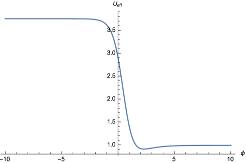
Figure 1: Qualitative shape of the total effective scalar potential $U_{\rm total}$ (44) as function of the “inflaton”$\varphi$ for fixed Higgs-like $\sigma$ (when $M_{0}\sigma^{*}\sigma\leq M_{1}$).

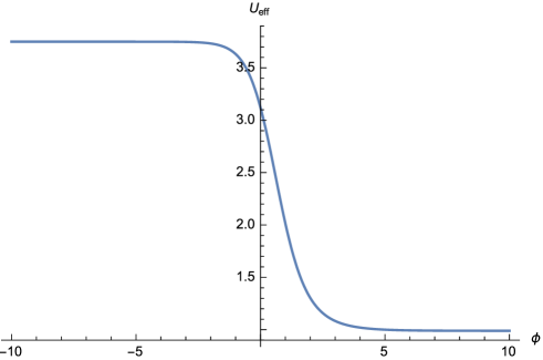
Figure 2: Qualitative shape of the total effective scalar potential $U_{\rm total}$ (44) as function of the “inflaton”$\varphi$ for fixed Higgs-like $\sigma$ (when $M_{0}\sigma^{*}\sigma\geq M_{1}$).

In the (-) flat “inflaton” region the effective scalar field potential reduces to:

$${\mathcal{U}}(\varphi,\sigma={\rm fixed})\simeq\frac{1}{4\epsilon\chi_{2}}\quad\longrightarrow\quad{\mathcal{U}}_{\rm total}\simeq{\mathcal{U}}^{(-)}_{\rm total}=\frac{1}{4\epsilon\chi_{2}}\;,$$ (45)

implying that all terms containing $\varphi$ and $\sigma$ disappear from the Einstein-frame Lagrangian (36). Thus, there is no $\sigma$-field potential and, therefore, no electroweak spontaneous breakdown in the (-) flat “inflaton” region.

From (40) the first relation (45) implies $f_{\rm eff}=0$. Recalling that $f_{\rm eff}$, the effective coupling constant of the square-root Maxwell term, measures the charge-confining strength according to [14, 9], we conclude that there is confinement is suppressed in the (-) flat “inflaton” region.

In the (+) flat “inflaton” region the effective scalar field potential becomes:

$${\mathcal{U}}(\varphi,\sigma)\simeq{\mathcal{U}}_{(+)}(\sigma)=\frac{\bigl{(}M_{0}^{2}\sigma^{*}\sigma-M_{1}\bigr{)}^{2}}{4\chi_{2}\bigl{[}M_{2}+\epsilon\bigl{(}M_{0}^{2}\sigma^{*}\sigma-M_{1}\bigr{)}^{2}\bigr{]}}$$ (46)

$$\longrightarrow\quad{\mathcal{U}}_{\rm total}(\varphi,\sigma)\simeq{\mathcal{U}}^{(+)}_{\rm total}(\sigma)=\frac{{\mathcal{U}}_{(+)}(\sigma)(1-\epsilon e^{2}f_{0}^{2})+e^{2}f_{0}^{2}/4\chi_{2}}{1+\epsilon e^{2}f_{0}^{2}\bigl{(}1-4\epsilon\chi_{2}{\mathcal{U}}_{(+)}(\sigma)\bigr{)}}$$ (47)

producing a dynamically generated nontrivial vacuum for the Higgs-like field:

$$|\sigma_{\rm vac}|=\sqrt{M_{1}}/M_{0}\;,$$ (48)

i.e., we obtain “gravity-inflaton-assisted” electroweak spontaneous breakdown in the (+) flat “inflaton” region.

At the Higgs vacuum we have dynamically generated vacuum energy density (cosmological constant):

$${\mathcal{U}}^{(+)}_{\rm total}(\sigma_{\rm vac})\equiv 2\Lambda_{(+)}=\epsilon e^{2}f_{0}^{2}\Bigl{[}4\epsilon\chi_{2}\bigl{(}1+\epsilon e^{2}f_{0}^{2}\bigr{)}\Bigr{]}^{-1}\;.$$ (49)

The effective confinement-strength coupling constant:

$$f_{\rm eff}\simeq f_{(+)}=f_{0}\bigl{(}1-4\epsilon\chi_{2}{\mathcal{U}}_{(+)}(\sigma)\bigr{)}>0\;,$$ (50)

therefore we obtain “gravity-inflaton-assisted” charge confinement in the (+) flat “inflaton” region.

As seen from Fig.1 or Fig.2, the heights of the two flat “inflaton” regions of the total scalar potential, i.e., the corresponding vacuum energies are given by (45) and (49), respectively:

$${\mathcal{U}}^{(-)}_{\rm total}=\frac{1}{4\epsilon\chi_{2}}\quad,\quad{\mathcal{U}}^{(+)}_{\rm total}(\sigma_{\rm vac})\equiv 2\Lambda_{(+)}=\epsilon e^{2}f_{0}^{2}\Bigl{[}4\epsilon\chi_{2}\bigl{(}1+\epsilon e^{2}f_{0}^{2}\bigr{)}\Bigr{]}^{-1}\;.$$ (51)

Thus, the $(-)$ and the $(+)$ flat “inflaton” regions of the effective “inflaton” potential with a very large and a very small height, respectively, can be accordingly identified as describing the “early” (“inflationary”) and “late” (today’s dark energy dominated) epoch of the universe provided we take the following numerical values for the parameters in order to conform to the PLANCK data [24, 25]:

$${\mathcal{U}}^{(-)}_{\rm total}\sim 10^{-8}M_{\rm Pl}^{4}\to\epsilon\chi_{2}\sim 10^{8}M_{\rm Pl}^{-4}\;\;,\;\;\Lambda_{(+)}\sim 10^{-122}M_{\rm Pl}^{4}\to\frac{e^{2}f_{0}^{2}}{\chi_{2}}\sim 10^{-122}M_{\rm Pl}^{4}\;,$$ (52)

where $M_{\rm Pl}$ is the Planck mass scale.

From the Higgs v.e.v. $|\sigma_{\rm vac}|=\sqrt{M_{1}}/M_{0}$ and the Higgs mass $\frac{M_{1}M_{0}^{2}}{4\chi_{2}M_{2}}$ resulting from the dynamically generated Higgs-like potential ${\mathcal{U}}^{(+)}_{\rm total}(\sigma)$ (47) we find:

$$M_{0}\sim M_{\rm EW}\;\;,\;\;M_{1,2}\sim M_{\rm EW}^{4}\;,$$ (53)

where $M_{\rm EW}\sim 10^{-16}M_{\rm Pl}$ is the electroweak mass scale.

5 5. Conclusions and Outlook

Here we have proposed a non-canonical model of $f(R)=R+R^{2}$ gravity coupled to the “inflaton” and the bosonic part of the standard particle model, incorporating two main building blocks – employing the formalism of non-Riemannian spacetime volume forms (generally covariant metric-independent volume elements) as well as introducing a special strongly non-linear gauge field with a square-root of the usual Maxwell/Yang-Mills kinetic term simulating QCD-like confinement dynamics. Due to the special interplay of the dynamics of the above principal ingredients our model is capable of producing in the Einstein frame:

• Unified “quintessential” description of the evolution of the “early” and “late” universe due to a natural dynamical generation of vastly different vacuum energy densities thanks to the auxiliary non-Riemannian volume-form antisymmetric tensor gauge fields;

• gravity-inflaton-assisted dynamical generation of Higgs-like electroweak spontaneous symmetry breaking effective scalar potential in the “late” universe, as well as gravity-inflaton-assisted charge confinement mechanism through the “square-root” nonlinear gauge field;

• Gravity-inflaton-induced suppression of electroweak spontaneous symmetry breaking, as well as gravity-inflaton-induced deconfinement in the “early” universe.

• Apart from the cosmological implications discussed above, the non-Riemannian volume-form formalism has further physically relevant applications such as producing a novel mechanism for supersymmetric Brout-Englert-Higgs effect in supergravity through dynamical generation of a cosmological constant, which triggers spontaneous supersymmetry breaking and dynamical gravitino mass generation [8, 26].

Let us also note that the QCD-simulating “square-root” nonlinear gauge field when interacting with gravity produces several other interesting effects:

(a) black holes with an additional constant background electric field exercising confining force on charged test particles even when the black hole itself is electrically neutral [27];

(b) Coupling to a charged lightlike brane produces a charge-“hiding” lightlike thin-shell wormhole, where a genuinely charged matter source is detected as electrically neutral by an external observer [28].

(c) Coupling to two oppositely charged lightlike brane sources produces a two-“throat” lightlike thin-shell wormhole displaying a genuine QCD-like charge confinement, i.e., the whole electric flux is trapped within a tube-like spacetime region connected the two charged lightlike branes [28].

(d) Charge confining gravitational electrovacuum shock wave [29].

The present model needs some further improvements. First of all it is necessary to avoid getting an unnaturally small value for the effective confinement strength coupling constant $f_{0}$ in the “late” universe resulting from the second relation (52) (the latter was needed for compatibility with the PLANCK data [24, 25] for the value of today’s cosmological constant).

Further important task must be the inclusion of the fermions in order to incorporate more faithfully the full standard particle model. To this end we can follow the steps outlined in several previous papers by some of us [30, 31, 32] devoted to the study of modified gravity within the non-Riemannian volume element formalism coupled to fermionic matter fields.

6 ACKNOWLEDGMENTS

We gratefully acknowledge support of our collaboration through the academic exchange agreement between the Ben-Gurion University in Beer-Sheva, Israel, and the Bulgarian Academy of Sciences. E.N. and E.G. have received partial support from European COST actions MP-1405 and CA-16104, and from CA-15117 and CA-16104, respectively. E.N. and S.P. are also thankful to Bulgarian National Science Fund for support via research grant DN-18/1.

References

- [1] E. Kolb and M. Turner, “The Early Universe” (Addison Wesley, 1990).
- [2] A. Linde, “Particle Physics and Inflationary Cosmology”, (Harwood, Chur, Switzerland, 1990).
- [3] A. Guth, “The Inflationary Universe” (Addison-Wesley, 1997).
- [4] A. Liddle and D. Lyth, “Cosmological Inflation and Large-Scale Structure” (Cambridge Univ. Press, 2000).
- [5] S. Dodelson, “Modern Cosmology” (Acad. Press, 2003).
- [6] V. Mukhanov, “Physical Foundations of Cosmology” (Cambridge Univ. Press, 2005).
- [7] S. Weinberg, “Cosmology” (Oxford Univ. Press, 2008).
- [8] E. Guendelman, E. Nissimov and S. Pacheva, Bulg. J. Phys. 41, 123 (2014) (arXiv:1404.4733).
- [9] E. Guendelman, E. Nissimov and S. Pacheva, Int. J. Mod. Phys. A30, 1550133 (2015) (arXiv:1504.01031).
- [10] E. Guendelman, Mod. Phys. Lett. A14 1043-1052 (1999) (arXiv:gr-qc/9901017).
- [11] E. Guendelman and A. Kaganovich, Phys. Rev. D60 065004 (1999) (arXiv:gr-qc/9905029).
- [12] E. Guendelman, E. Nissimov and S. Pacheva, Int. J. Mod. Phys. D25, 1644008 (2016) (1603.06231).
- [13] J. Bekenstein, Found. Phys. 16, 409 (1986).
- [14] P. Gaete and E. Guendelman, Phys. Lett. B640 201-204 (2006) (arXiv:hep-th/0607113).
- [15] G. ’t Hooft, Nucl. Phys. B (Proc. Suppl.) 121 333-340 (2003) (arXiv:0208054[hep-th]).
- [16] E. Guendelman, E. Nissimov and S. Pacheva, in Jacob Bekenstein Memorial Volume (World Scientific, 2018), to be published, (arXiv:1804.07925.
- [17] E. Eichten, K. Gottfried, T. Kinoshita, J. Kogut, K. Lane and T.-M. Yan, Phys. Rev. Lett. 34, 369-372 (1975).
- [18] W. Buchmüller (ed.), “Quarkonia”, Current Physics Sources and Comments, vol.9, North Holland (1992).
- [19] M. Karliner, B. Keren-Zur, H. Lipkin and J. Rosner, Ann. of Phys. 324, 2-15 (2009) (0804.1575[hep-ph]).
- [20] T. Chiba, T.Okabe and M. Yamaguchi, Phys. Rev. D62, 023511 (2000) (arXiv:astro-ph/9912463).
- [21] C. Armendariz-Picon, V. Mukhanov and P. Steinhardt, Phys. Rev. Lett. 85, 4438 (2000) (arXiv:astro-ph/0004134).
- [22] C. Armendariz-Picon, V. Mukhanov and P. Steinhardt, Phys. Rev. D63, 103510 (2001) (arXiv:astro-ph/0006373).
- [23] T. Chiba, Phys. Rev. D66, 063514 (2002) (arXiv:astro-ph/0206298).
- [24] R. Adam et al. (Planck Collaboration), Astron. Astrophys. 571, A22 (2014) (arXiv:1303.5082 [astro-ph.CO]).
- [25] R. Adam et al. (Planck Collaboration), Astron. Astrophys. 586, A133 (2016) (arXiv:1409.5738 [astro-ph.CO]).
- [26] E. Guendelman, E. Nissimov and S. Pacheva, in Eight Mathematical Physics Meeting, ed. by B. Dragovich and I. Salom (Belgrade Inst. Phys. Press, 2015), pp. 105-115 (arXiv:1501.05518).
- [27] E. Guendelman, E. Nissimov and S. Pacheva, Phys. Lett. 704B, 230 (2011), erratum Phys. Lett. 705B, 545 (2011) (arXiv:1108.0160).
- [28] E. Guendelman, E. Nissimov and S. Pacheva, Int. J. Mod. Phys. A26, 5211 (2011) (arXiv:1109.0453).
- [29] E. Guendelman, E. Nissimov and S. Pacheva, Mod. Phys. Lett. A29, 1450020 (2014) (arXiv:1310.1558).
- [30] E. Guendelman and A. Kaganovich, Mod. Phys. Lett. A17, 1227 (2002) (arXiv:hep-th/0110221).
- [31] E. Guendelman and A. Kaganovich, Int. J. Mod. Phys. A19, 5325 (2004) (arXiv:gr-qc/0408026).
- [32] E. Guendelman and A. Kaganovich, Int. J. Mod. Phys. A21, 4373 (2006) (arXiv:gr-qc/0603070).