Derivative Corrections to the Trapezoidal Rule

Abstract

Extensions to the trapezoidal rule using derivative information are studied for periodic integrands and integrals along the entire real line. Integrands which are analytic within a half plane or within a strip containing the path of integration are considered. Derivative-free error bounds are obtained. Alternative approaches to including derivative information are discussed.

65D32

1 Introduction

The trapezoidal rule for numerical quadrature is remarkably accurate when applied to periodic integrands or integrals along the entire real axis. We consider here extensions of this method where derivative information is taken into account. Trefethen and Weideman [11] have recently produced a thorough review of the trapezoidal rule, but did not cover derivative information. In this work, we generalize the term “trapezoidal rule” to mean any numerical quadrature scheme that utilizes information about the function being integrated at equally-spaced quadrature points, with the rule treating every point on the same footing (e.g., with equal weight for a typical linear rule).

The use of derivative information in numerical quadrature has been reviewed by Davis and Rabinowitz [4, section 2.8]; for a more recent example, see Burg [3]. The case for utilizing derivative information in quadrature becomes compelling when derivatives at the quadrature points can be calculated with significantly less effort than the alternative of evaluating the integrand at additional quadrature points. This may be the case, for example, if the integrand satisfies a differential equation. The derivative corrections may also be useful for error analysis in high-precision numerical quadrature [1]. Davis and Rabinowitz also noted that the calculation of derivatives often requires additional “pencil work” – a complication that has now been removed for the most part by the advent of computer algebra. The application derivative information to the trapezoidal rule was pioneered by Kress for periodic functions [8] and functions on the real line that are analytic within a strip containing the path of integration [9].

This paper is organized as follows. We first consider in section 2 periodic functions which are analytic either within a half plane or a strip, with examples presented in sections 3 and 4. We then consider in section 5 functions on the real line which are analytic within a strip or half plane. In section 6 we consider the limit in which a large number of derivatives are included and finally in section 7 some other approaches to taking derivative information into account are discussed. To the best of our knowledge, the results for functions that are analytic within a half plane and the material in sections 6 and 7 are new. We have utilized the notation of Trefethen and Weideman [11] to the extent possible and the proofs given below draw significantly from their paper.

2 Integrals over a Periodic Interval

Let $v$ be a real or complex function with period $2\pi$ on the real line and consider the definite integral

(1) $$I=\int_{0}^{2\pi}v(\theta)\,d\theta.$$

The trapezoidal rule approximation for this integral is given by [11, (3.2)]

(2) $$I_{N}=\frac{2\pi}{N}\sum_{j=1}^{N}\,v(\theta_{j}),$$

where $N>0$ is the number of quadrature points and $\theta_{j}=2\pi j/N$.

Assuming that $v$ is $D$-times differentiable, we define a generalized trapezoidal rule approximation that takes into account derivative information at the quadrature points via

(3) $$I_{N,D}=\frac{2\pi}{N}\sum_{j=1}^{N}\sum_{k=0}^{D}\left(\frac{1}{N}\right)^{k}A_{k,D}\,v^{(k)}(\theta_{j}),$$

where $D$ is the maximum derivative order included and $A_{k,D}$ are constants, with $A_{0,D}=1$. Note that we have defined $A_{k,D}$ to be independent of the particular point $j$, which is an intuitive choice based on the symmetry of the points but not a requirement. For simplicity, we have assumed that no derivatives are skipped in the sum over $k$, but this also is not a requirement. The factor of $(1/N)^{k}$ has been inserted for convenience: with this factor, the prescriptions for defining $A_{k,D}$ given below lead to $A_{k,D}$ being independent of $N$. We observe that for $D=0$, the standard trapezoidal rule for periodic functions (2), which does not use derivatives, is recovered.

Theorem 2.1.

Suppose $v$ is $2\pi$-periodic and analytic and satisfies $|v(\theta)|\leq M$ in the half-plane $\operatorname{Im}\,\theta>-a$ for some $a>0$. Further suppose that $D$ is a positive integer, $k$ is an integer with $0\leq k\leq D$, and

(4) $$i^{k}A_{k,D}=\frac{(-1)^{D}}{D!}s(D+1,k+1),$$

where $s(D+1,k+1)$ are the Stirling numbers of the first kind. Then for $N>0$ and $I_{N,D}$ as defined in (3)

(5) $$|I_{N,D}-I|\leq\frac{2\pi M}{(e^{aN}-1)^{D+1}}$$

and the constant $2\pi$ is as small as possible.

Proof 2.2.

Since $v$ is analytic, it has the uniformly and absolutely convergent Fourier series

(6) $$v(\theta)=\sum_{\ell=-\infty}^{\infty}c_{\ell}e^{i\ell\theta},$$

where the coefficients are given by

(7) $$c_{\ell}=\frac{1}{2\pi}\int_{0}^{2\pi}e^{-i\ell\theta}v(\theta)\,d\theta.$$

From (1) and (7), we also have

(8) $$I=2\pi c_{0}.$$

We define the auxiliary function

(9) $$v_{N,D}(\theta)=\sum_{k=0}^{D}\left(\frac{1}{N}\right)^{k}A_{k,D}\,v^{(k)}(\theta),$$

which is also analytic and $2\pi$ periodic. Using the expansion (6) we can then write

(10) $$v_{N,D}(\theta)=\sum_{\ell=-\infty}^{\infty}\sum_{k=0}^{D}A_{k,D}\left(\frac{i\ell}{N}\right)^{k}c_{\ell}e^{i\ell\theta},$$

where we have used the fact that (6) is absolutely convergent to justify differentiating and re-ordering the summation and $\ell^{k}$ is understood to be unity if $\ell=k=0$. Using the definition (9), we may write (3) as

(11) $$I_{N,D}=\frac{2\pi}{N}\sum_{j=1}^{N}v_{N,D}(\theta_{j}),$$

which when combined with (8) and (10) gives

(12) $$I_{N,D}-I=\frac{2\pi}{N}\sum_{j=1}^{N}\sum_{\ell=1}^{\infty}\sum_{k=0}^{D}A_{k,D}\left[\left(\frac{i\ell}{N}\right)^{k}c_{\ell}e^{i\ell\theta_{j}}+\left(\frac{-i\ell}{N}\right)^{k}c_{-\ell}e^{-i\ell\theta_{j}}\right].$$

Using the fact that

(13) $$\sum_{j=1}^{N}e^{i\ell\theta_{j}}=\left\{\begin{array}[]{ll}N&\ell\bmod N=0\\ 0&\text{otherwise}\end{array}\right.$$

and redefining the index $\ell\rightarrow\ell N$, (12) becomes

(14) $$I_{N,D}-I=2\pi\sum_{\ell=1}^{\infty}\sum_{k=0}^{D}A_{k,D}\left[(i\ell)^{k}c_{\ell N}+(-i\ell)^{k}c_{-\ell N}\right].$$

The bound $|v(\theta)|\leq M$ for $\operatorname{Im}\,\theta>-a$ provides a constraint on the coefficients $c_{\ell}$, which may be quantified by considering various integration contours for (7). For $\ell\geq 0$, shifting the interval [0,$2\pi$] downward by a distance $a^{\prime}<a$ into the lower half plane shows $|c_{\ell}|\leq Me^{-\ell a}$, where we have taken $a^{\prime}$ arbitrarily close to $a$ and noted that the contributions from the sides of the contour vanish by periodicity. For $\ell<0$, the interval may be shifted upwards an arbitrary distance $b$, which leads to $|c_{\ell}|\leq Me^{\ell b}$. Since $b$ is arbitrary, $c_{\ell}$ must vanish in this case. Summarizing, we have

(15a) $$|c_{\ell}| \leq Me^{-\ell a} \ell\geq 0\quad\quad\text{and}$$

(15b) $$c_{\ell} =0 \ell<0.$$

With this restriction on the Fourier coefficients, (14) now becomes

(16) $$I_{N,D}-I=2\pi\sum_{\ell=1}^{\infty}\sum_{k=0}^{D}(i\ell)^{k}A_{k,D}\,c_{\ell N}.$$

In view of the geometric decay of the Fourier coefficients, we will choose the remaining $A_{k,D}$ to eliminate as many low-order Fourier coefficients as possible from the right-hand-side of (16). We thus now require

(17) $$\sum_{k=1}^{D}(i\ell)^{k}A_{k,D}=-1\quad\quad 1\leq\ell\leq D.$$

This is an inhomogeneous Vandermonde system for $i^{k}A_{k,D}$, which must have a unique non-trivial solution. It is useful to consider the quantity

(18) $$E_{\ell,D}=\sum_{k=0}^{D}(i\ell)^{k}A_{k,D}=\prod_{k=1}^{D}(1-\ell/k),$$

where the factorization results from the definition $A_{0,D}=1$ and the observation that $E_{\ell,D}$ is a polynomial in $\ell$ of degree $D$ that according to the definition (17) has zeros for the first $D$ positive integers. We see that $i^{D}A_{D,D}=(-1)^{D}/D!$ and that

(19) $$E_{\ell,D}=(1-\ell/D)E_{\ell,D-1},\quad D\geq 1,$$

which implies a recurrence formula:

(20) $$i^{k}A_{k,D}=i^{k}A_{k,D-1}-\frac{i^{k-1}A_{k-1,D-1}}{D},\quad 1\leq k\leq D-1,D\geq 1.$$

The coefficients may also be represented by

(21) $$i^{k}A_{k,D}=\frac{(-1)^{D}}{D!}s(D+1,k+1),$$

where $s(D+1,k+1)$ are the Stirling numbers of the first kind [2]. This result can be confirmed by noting that it correctly yields $A_{0,D}=1$, $i^{D}A_{D,D}=(-1)^{D}/D!$, and, using the recurrence formula for the Stirling numbers of the first kind [2, (26.8.18)], satisfies (20).

Using the factorized form of $E_{\ell,D}$ we also find

(22) $$E_{\ell,D}=(-1)^{D}\binom{\ell-1}{D},\quad\ell>D$$

and thus (16) becomes

(23) $$I_{N,D}-I=2\pi\sum_{\ell=D+1}^{\infty}c_{\ell N}E_{\ell,D}.$$

Using the bound on the Fourier coefficients (15a) and (22), we then obtain

(24) $$|I_{N,D}-I|\leq 2\pi M\sum_{\ell=D+1}^{\infty}e^{-a\ell N}\binom{\ell-1}{D},$$

which upon summing the series is (5).

To show the sharpness of the constant $2\pi$ in the bound (5) we consider

(25) $$v(\theta)=e^{i(D+1)N\theta},$$

which has $I=0$ and has vanishing Fourier coefficients except for $c_{(D+1)N}=1$ and leads to

(26) $$I_{N,D}-I=2\pi E_{D+1,D}=2\pi\,(-1)^{D}.$$

The sharp bound on this $v(\theta)$ for $\operatorname{Im}\,\theta>-a$ is

(27) $$|v(\theta)|<M=e^{a(D+1)N}.$$

The bound (5) is seen to be asymptotic to the exact result for $|I_{N,D}-I|$ as $N\rightarrow\infty$.

This result is an extension of Theorem 3.1 of Trefethen and Weideman [11], which makes the same assumptions regarding $v(\theta)$ and finds that the error of the usual trapezoidal rule to be $|I_{N,0}-I|=O(e^{-aN})$ for $N\rightarrow\infty$. When derivative information is included, we find that the rate of geometric convergence can be improved to $O(e^{-a(D+1)N})$. Practically speaking, one thus expects the number of quadrature points needed to achieve a given level of precision to be reduced by a factor of $(D+1)$ when derivative information is considered.

We also observe that the bound (5) implies

(28) $$\lim_{D\rightarrow\infty}|I_{N,D}-I|=0\quad a,N>0,$$

where the convergence is geometric. However, there are practical issues when $D$ is large, as there must be large cancellations in $I_{N,D}$ in this limit: consider, for example,

(29) $$iA_{1,D}=\sum_{k=1}^{D}\frac{1}{k}$$

which diverges as $D\rightarrow\infty$.

In Table 1 we present $A_{k,D}$ for $D=1,$ 2, and 3. A numerical example of this quadrature formula is provided below in section 3.

Table 1: The constants $A_{k,D}$ defined by (4), for the three lowest $D$ values.

D	$A_{1,D}$	$A_{2,D}$	$A_{3,D}$
1	$i$	-	-
2	$3i/2$	$-1/2$	-
3	$11i/6$	$-1$	$-i/6$

Due to the restrictions on $v(\theta)$, this theorem is not applicable to real integrands, unless they are a constant. We will next consider a similar extension to Theorem 3.2 of Trefethen and Weideman [11], which has a less restrictive condition on $v(\theta)$ and may be applied to real integrands.

Theorem 2.3.

Suppose $v$ is $2\pi$-periodic and analytic and satisfies $|v(\theta)|\leq M$ in the strip $|\operatorname{Im}\,\theta|<a$ for some $a>0$. Further suppose that $D$ is a positive even integer, $\ell$ and $m$ are integers with $1\leq\ell,m\leq D/2$, $B_{0,D}=1$, $B_{2m-1,D}=0$, and $B_{2m,D}$ are the solution to the Vandermonde system

(30) $$\sum_{m=1}^{D/2}(-1)^{m}\ell^{2m}B_{2m,D}=-1.$$

Then with $I_{N,D}$ as defined in (3) with $B_{k,D}$ replacing $A_{k,D}$ therein and $N>0$

(31a) $$|I_{N,D}-I|\leq\frac{4\pi M}{(1-e^{-aN})^{D+1}}\left|\sum_{\ell=D/2+1}^{D+1}(-1)^{\ell}\binom{D+1}{\ell}e^{-a\ell N}\right|,$$

and for $$N\rightarrow\infty$$

(31b) $$|I_{N,D}-I|\leq 4\pi M\binom{D+1}{D/2}e^{-a(D/2+1)N}\left[1+O(e^{-aN})\right],$$

and the constant $4\pi$ is as small as possible.

Proof 2.4.

The proof is very similar to Theorem 2.1. Equations (6)-(14) continuing to hold, with $B_{k,D}$ replacing $A_{k,D}$. The bound $|v(\theta)|\leq M$ for $|\operatorname{Im}\,\theta|<a$ provides a weaker constraint on the Fourier coefficients. For $\ell\geq 0$, the bound on $c_{\ell}$ is unchanged. For $\ell\leq 0$, the integration interval in (7) may be shifted upward by a distance $a^{\prime}<a$ which leads to $|c_{\ell}|\leq Me^{\ell a}$. Summarizing, we now have

(32) $$|c_{\ell}|\leq Me^{-|\ell|a}.$$

In this case, the remainder (14) now becomes

(33) $$I_{N,D}-I=2\pi\sum_{\ell=1}^{\infty}\sum_{k=0}^{D}B_{k,D}\left[(i\ell)^{k}c_{\ell N}+(-i\ell)^{k}c_{-\ell N}\right].$$

For a given value of $\ell$ in (33), the Fourier coefficients appear in pairs, $c_{\ell N}$ and $c_{-\ell N}$, that are of comparable magnitude. We will again choose the remaining $B_{k,D}$ to eliminate as many of the low-order Fourier components as possible. In order make the contribution of a particular pair vanish, we require

(34a) $$1+\sum_{k=1}^{D}(i\ell)^{k}B_{k,D}=0\quad\quad\text{and}$$

(34b) $$1+\sum_{k=1}^{D}(-i\ell)^{k}B_{k,D}=0.$$

Adding or subtracting these equations decouples the even and odd coefficients:

(35a) $$\sum_{m=1}^{D/2}(-1)^{m}\ell^{2m}B_{2m,D}=-1\quad\quad\text{and}$$

(35b) $$\sum_{m=1}^{D/2}(-1)^{m}\ell^{2m-1}B_{2m-1,D}=0,$$

where were have now restricted $D$ to be even. Because there are two equations for each $\ell$ value, this assumption allows us to match the number of equations to the number of unknown $B_{k,D}$ by considering $\ell$ values from one up to $D/2$. Since (35a) is an inhomogeneous real Vandermonde system for $(-1)^{m}B_{2m,D}$, it has a unique non-trivial solution. For the odd coefficients, (35b) is a homogeneous Vandermonde system for $(-1)^{m}B_{2m-1,D}$ and its only solution is the trivial one,

(36) $$B_{2m-1,D}=0,\quad\quad 1\leq m\leq D/2.$$

We note that if $D$ is permitted to be odd there is ambiguity in the definition of $B_{2m,D}$ because considering $\ell$ values up to $(D-1)/2$ does not provide enough equations to uniquely determine the coefficients, but increasing the maximum $\ell$ value by one overdetermines them.

It is useful to consider the quantity

(37) $$F_{\ell,D}=\sum_{m=0}^{D/2}(-1)^{m}\ell^{2m}B_{2m,D}=\prod_{m=1}^{D/2}\left[1-(\ell/m)^{2}\right],$$

where the product form results from noting that $F_{\ell,D}$ is a polynomial in $\ell^{2}$ of degree $D/2$ with $F_{0,D}=1$ and that the fact that, according to (35a), $F_{\ell,D}$ is zero for when $\ell$ is one of the first $D/2$ positive integers. In addition, we note that $F_{\ell,D}$ is nonzero and monotonically increasing in absolute value for $\ell>D/2$. From this equation, one can observe at once that

(38) $$B_{2,D} =\sum_{m=1}^{D/2}\frac{1}{m^{2}}\quad\quad\text{and}$$

(39) $$B_{D/2,D} =\frac{1}{[(D/2)!]^{2}}.$$

Following Kress [8, 9], a recurrence relation for the $B_{2m,D}$ coefficients may be derived by noting

(40) $$F_{\ell,D}=\left[1-\left(2\ell/D\right)^{2}\right]F_{\ell,D-2},\quad D\geq 2$$

which provides

(41) $$B_{2m,D}=B_{2m,D-2}+(2/D)^{2}B_{2m-2,D-2},\quad 1\leq m\leq D/2,D\geq 2.$$

Using the factorized form of $F_{\ell,D}$, one readily finds

(42) $$F_{\ell,D}=(-1)^{D/2}\binom{\ell+D/2}{D/2}\binom{\ell-1}{D/2},\quad\ell>D/2$$

With this definition for $F_{\ell,D}$, (33) becomes

(43) $$I_{N,D}-I=2\pi\sum_{\ell=D/2+1}^{\infty}(c_{\ell N}+c_{-\ell N})F_{\ell,D}.$$

Using the bound on the Fourier coefficients (32), we then obtain

(44) $$I_{N,D}-I=4\pi M\left|\sum_{\ell=D/2+1}^{\infty}e^{-a\ell N}F_{\ell,D}\right|,$$

where we have used the fact that all $F_{\ell,D}$ have the same sign for $\ell>D/2$ to justify moving the absolute value outside of the summation. Making use of the identity

(45) $$\begin{split}(-1)^{D/2}\sum_{\ell=D/2+1}^{\infty}&\binom{\ell+D/2}{D/2}\binom{\ell-1}{D/2}e^{-a\ell N}\\ =&\frac{-1}{(1-e^{-aN})^{D+1}}\sum_{\ell=D/2+1}^{D+1}(-1)^{\ell}\binom{D+1}{\ell}e^{-a\ell N},\end{split}$$

one obtains (31a), which is asymptotically equivalent to the bound (31b) as $N\rightarrow\infty$.

To show the sharpness of the constant $4\pi$ in the bounds (31a) and (31b), we consider

(46) $$v(\theta)=2\cos(D/2+1)N\theta,$$

which has $I=0$ and vanishing Fourier coefficients except for $c_{\pm(D/2+1)N}=1$ and leads to

(47) $$I_{N,D}-I=4\pi\sum_{m=0}^{D/2}(-1)^{m}(D/2+1)^{2m}B_{2m,D}=4\pi(-1)^{D/2}\binom{D+1}{D/2}.$$

The sharp bound on this $v(\theta)$ for $|\operatorname{Im}\,\theta|<a$ is

(48) $$|v(\theta)|<M=2\cosh(D/2+1)Na.$$

The bounds (31a) and (31b) are both seen to be asymptotic to the exact result for $|I_{N,D}-I|$ as $N\rightarrow\infty$.

Theorem 3.2 of Trefethen and Weideman [11], which makes the same assumptions regarding $v(\theta)$, finds that the error of the usual trapezoidal rule to be $|I_{N,0}-I|=O(e^{-aN})$ for $N\rightarrow\infty$. When derivative information is included, we find that the rate of geometric convergence can be improved to $|I_{N,D}-I|=O(e^{-a(D/2+1)N})$. Interestingly, the coefficients of the odd derivatives in (3) are found vanish – which implies they are not useful for improving the accuracy of the trapezoidal rule in this case. This quadrature rule appears to have been first derived by Kress [8]. Our error bound is somewhat tighter, as Kress (in our notation) utilized

(49) $$\left|\sum_{\ell=D/2+1}^{D+1}(-1)^{\ell}\binom{D+1}{\ell}e^{-a\ell N}\right|\leq 2^{D}e^{-a(D/2+1)N},$$

which is only sharp for $D=0$. The leading behavior of the error bound (31b) is consistent with the findings of Wilhelmsen [13]. A numerical demonstration of this quadrature rule is provided below in section 4.

Table 2: The constants $B_{2m,D}$ defined by (30) and $F_{D/2+1,D}$ defined by (42) which are applicable to Theorems 2.3 and 5.1, for the three lowest even $D$ values.

D	$B_{2,D}$	$B_{4,D}$	$B_{6,D}$	$F_{D/2+1,D}=(-1)^{D/2}\binom{D+1}{D/2}$
2	1	-	-	-3
4	5/4	1/4	-	10
6	49/36	7/18	1/36	-35

The polylogarithm function

(50) $$\operatorname{Li}_{-k}(z)=\sum_{\ell=1}^{\infty}\ell^{k}z^{\ell},\quad|z|<1$$

may be used to write remainder bound in third form, in addition to (31a) or (44) with (42) for $F_{\ell,D}$. Using (37) for $F_{\ell,D}$ in (44) with (50), we have

(51) $$\sum_{\ell=D/2+1}^{\infty}e^{-a\ell N}F_{\ell,D}=\sum_{m=0}^{D/2}(-1)^{m}B_{2m,D}\operatorname{Li}_{-2m}(e^{-aN}).$$

For the case $D=2$, we have $B_{2,2}$=1 and (31a) becomes

(52) $$|I_{N,2}-I|\leq 4\pi M\frac{e^{-2aN}(3-e^{-aN})}{(1-e^{-aN})^{3}}.$$

In Table 2 we present $B_{2m,D}$ and $F_{D/2+1,D}$ for $D=2,$ 4, and 6.

3 Example: Integral of a Periodic Complex Function

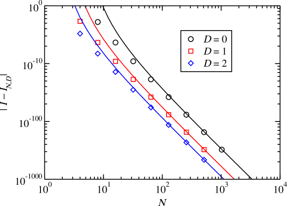
Figure 1: The actual (points) and predicted (curves) convergence of the generalized trapezoidal rule (3) using the coefficients corresponding to Theorem 2.1 given in Table 1, for $v(\theta)$ given by (53) with $e^{b}=2$.

Here we present an example using a complex periodic function that fulfills the requirements of Theorem 2.1:

(53) $$v(\theta)=\frac{1}{e^{b}+e^{i\theta}},$$

where $b$ is a positive real constant. This function has simple poles in the lower half plane at $\theta=2\pi(j+1/2)-ib$, where $j$ is any integer. We then have $0<a<b$, where $a$ defines the half plane in the conditions of Theorem 2.1. For $\operatorname{Im}\,\theta>-a$, the sharp upper bound on $|v(\theta)|$ is $M=(e^{b}-e^{a})^{-1}$. The error bound may be optimized by choosing $a$ to minimize the leading geometric term in (5), $2\pi Me^{-a(D+1)N}$. Using calculus, one thus obtains

$$a=b-\frac{1}{(D+1)N}+O(1/N^{2}),\quad N\rightarrow\infty\quad\text{and}$$

(54) $$|I_{N,D}-I|\leq 2\pi e(D+1)Ne^{-b[(D+1)N+1]}\left[1+O(1/N)\right],\quad N\rightarrow\infty.$$

The actual convergence results and this bound are plotted in Figure 1, for $e^{b}=2$. The expected geometric convergence and improvement from including derivative information are seen. For this $v(\theta)$, the exact error can be calculated via (23), which results in

(55) $$|I_{N,D}-I|=2\pi e^{-b[(D+1)N+1]}\left[1+O(1/N)\right],\quad N\rightarrow\infty.$$

We see that for large $N$, the error bound is a factor of $(D+1)Ne$ greater than the actual error.

4 Example: Integral of a Periodic Real Function

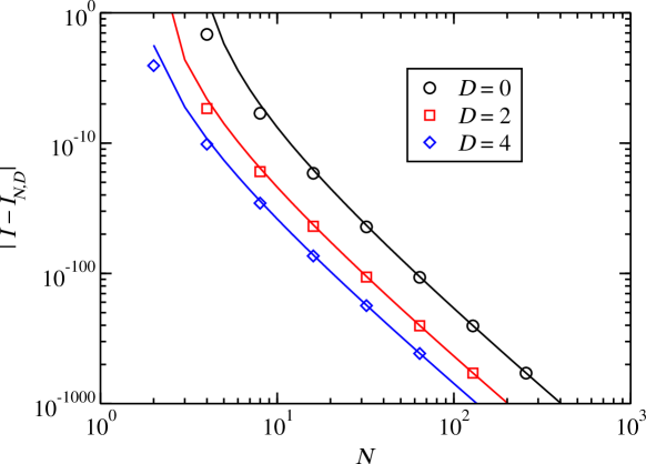
Figure 2: The actual (points) and predicted (curves) convergence of the generalized trapezoidal rule (3) using the coefficients corresponding to Theorem 2.3 given in Table 1, for $v(\theta)$ given by (56).

Here we present an example with a real integrand that fulfills the requirements of Theorem 2.3:

(56) $$v(\theta)=e^{\cos\theta},$$

an example also considered by Trefethen and Weideman [11]. We first note the remarkable accuracy that can be achieved with just a modest number of terms – for example, $N=4$ and $D=4$ results in

(57) $$I_{4,4}=\frac{\pi}{1024}\left(1101+553/e+474e\right)=7.9549265210781\ldots$$

where the first 11 digits are correct. In this case $v(\theta)$ is entire, with $|v(\theta)|$ unbounded as $\operatorname{Im}\,\theta\rightarrow\infty$. The sharp bound on $|v(\theta)|$ in the strip $|\operatorname{Im}\,\theta|<a$ is $M=e^{\cosh a}$. The leading geometric term in the error bound is $4\pi\binom{D+1}{D/2}Me^{-a(D/2+1)N}$, which may be minimized using calculus, resulting in

$$e^{a}=(D+2)N+O(1/N),\quad N\rightarrow\infty\quad\text{and}$$

(58) $$|I_{N,D}-I|\leq 4\pi\binom{D+1}{D/2}\left[\frac{e}{(D+2)N}\right]^{(D/2+1)N}\left[1+O(1/N)\right],\quad N\rightarrow\infty.$$

The actual convergence results and this bound are plotted in Figure 2, where the expected geometric convergence and improvement from including derivative information are seen.

5 Integrals on the Real Line

Let $w$ be a real or complex function on the real line and consider the definite integral

(59) $$I=\int_{-\infty}^{\infty}w(x)\,dx.$$

The trapezoidal rule approximation for this integral is given by [11, (5.2)]

(60) $$I_{h}=h\sum_{j=-\infty}^{\infty}w(x_{j}),$$

where $h>0$ and $x_{j}=jh$.

Assuming that $w$ is $D$-times differentiable, we define a generalized trapezoidal rule approximation that takes into account derivative information via

(61) $$I_{h,D}=h\sum_{j=-\infty}^{\infty}\sum_{k=0}^{D}\left(\frac{h}{2\pi}\right)^{k}B_{k,D}\,w^{(k)}(x_{j}),$$

where $D$ is the maximum derivative order included and $B_{k,D}$ are constants with $B_{0,D}=1$. We have assumed that $B_{k,D}$ is independent of $j$ and that no derivatives are skipped in the sum over $k$, neither of which is a requirement. The factor of $(h/2\pi)^{k}$ has been inserted for convenience, as it will lead to $B_{k,D}$ being independent of $h$. We observe that for $D=0$, the standard trapezoidal rule (60) is recovered.

Theorem 5.1.

Suppose $w$ is analytic in the strip $|\operatorname{Im}\,x|<a$ for some $a>0$, $w(x)\rightarrow 0$ uniformly as $|x|\rightarrow\infty$, and for some $M$, it satisfies

(62) $$\int_{-\infty}^{\infty}|w(x+ib)|dx\leq M$$

for all $b\in(-a,a)$. Further suppose that $D$ is a positive even integer, $\ell$ and $m$ are integers with $1\leq\ell,m\leq D/2$, $B_{0,D}=1$, $B_{2m-1,D}=0$, and $B_{2m,D}$ are the solution to the Vandermonde system

(63) $$\sum_{m=1}^{D/2}(-1)^{m}\ell^{2m}B_{2m,D}=-1.$$

Then for $h>0$, $I_{h,D}$ as defined in (61) exists and

(64a) $$|I_{h,D}-I|\leq\frac{2M}{(1-e^{-2\pi a/h})^{D+1}}\left|\sum_{\ell=D/2+1}^{D+1}(-1)^{\ell}\binom{D+1}{\ell}e^{-2\pi\ell a/h}\right|,$$

and for $$h\rightarrow 0$$

(64b) $$|I_{h,D}-I|\leq 2M\binom{D+1}{D/2}e^{-2\pi(D/2+1)a/h}\left[1+O(e^{-2\pi a/h})\right],$$

and the constant $2M$ is as small as possible.

Proof 5.2.

The proof is by residue calculus. We definite the auxiliary function

(65) $$w_{h,D}(x)=\sum_{k=0}^{D}\left(\frac{h}{2\pi}\right)^{k}B_{k,D}\,w^{(k)}(x).$$

The assumption that $w(x)\rightarrow 0$ uniformly as $|x|\rightarrow\infty$ implies by Cauchy integrals that the same holds true for $w^{(k)}(x)$ and $w_{h,D}(x)$. The function

(66) $$m(x)=-\frac{i}{2}\cot\frac{\pi x}{h}$$

has simple poles at $x=0,\pm h,\pm 2h,\ldots,$ all with residues equal to $h/(2\pi i)$. For convenience, we consider the sum in (61) to be symmetric, from $-n$ to $n$ with $n\rightarrow\infty$. Our arguments are trivially generalized to an arbitrary sum from $n_{-}$ to $n_{+}$, with $n_{-},n_{+}\rightarrow\infty$, as our reasoning do not depend upon the symmetry of the sum.

The residue theorem thus implies that for any positive integer $n$

(67) $$I_{h,D}^{[n]}=\int_{\Gamma}m(x)w(x)\,dx,$$

where $I_{h,D}^{[n]}$ is the truncated form of the generalized trapezoidal rule (61) and the clockwise contour $\Gamma$ encircles the poles in $[-nh,nh]$. We take $\Gamma$ to be the rectangular contour with vertices $\pm(n+\frac{1}{2})h+ia^{\prime}$ and $\pm(n+\frac{1}{2})-ia^{\prime}$ for any $a^{\prime}$ with $0<a^{\prime}<a$. This contour is depicted in Figure 5.1 of Trefethen and Weideman [11]. We can also write using Cauchy’s theorem that

(68) $$\int_{-(n+\frac{1}{2})h}^{(n+\frac{1}{2})h}w_{h,D}(x)\,dx=\int_{\Gamma_{-}}w_{h,D}(x)\,dx=-\int_{\Gamma_{+}}w_{h,D}(x)\,dx,$$

where $\Gamma_{-}$ and $\Gamma_{+}$ are the segments of $\Gamma$ with $\operatorname{Im}\,x\leq 0$ and $\operatorname{Im}\,x\geq 0$, respectively. Using the average of these two forms of (68) we can write

(69) $$h \sum_{j=-n}^{n}w_{h,D}(jh)-\int_{-(n+\frac{1}{2})h}^{(n+\frac{1}{2})h}w_{h,D}(x)\,dx$$

$$=-\frac{1}{2}\int_{\Gamma_{-}}(1+i\cot\frac{\pi x}{h})w_{h,D}(x)\,dx+\frac{1}{2}\int_{\Gamma_{+}}(1-i\cot\frac{\pi x}{h})w_{h,D}(x)\,dx$$

$$=-\int_{\Gamma_{-}}\frac{w_{h,D}(x)}{1-e^{2\pi ix/h}}\,dx+\int_{\Gamma_{+}}\frac{w_{h,D}(x)}{1-e^{-2\pi ix/h}}\,dx.$$

In the limit $n\rightarrow\infty$, the contributions of the vertical legs of the contours $\Gamma_{\pm}$ vanish. This can be seen by considering $|1+\exp(\mp 2\pi ix/h)|\geq 2$ on the vertical legs of $\Gamma_{\pm}$ and the decay properties of $w_{h,D}(x)$. We also have

(70) $$\int_{-\infty}^{\infty}w_{h,D}(x)\,dx =I+\sum_{k=1}^{D}\left(\frac{h}{2\pi}\right)^{k}B_{k,D}\int_{-\infty}^{\infty}w^{(k)}(x)\,dx$$

$$=I,$$

since for $k\geq 1$ the integrals on the right-hand side can be evaluated via integration by parts and the results vanish do to the decay properties of $w^{(k-1)}(x)$. In the limit $n\rightarrow\infty$, (69) thus becomes

(71) $$I_{h,D}-I=-\int_{-\infty-ia^{\prime}}^{\infty-ia^{\prime}}\frac{w_{h,D}(x)}{1-e^{2\pi ix/h}}\,dx-\int_{-\infty+ia^{\prime}}^{\infty+ia^{\prime}}\frac{w_{h,D}(x)}{1-e^{-2\pi ix/h}}\,dx.$$

We define

(72) $$f_{\pm}(x)=\frac{-1}{1-e^{\mp 2\pi ix/h}}=\sum_{\ell=1}^{\infty}e^{\pm 2\pi i\ell x/h},$$

where the geometric series representations are absolutely convergent along the respective paths of integration in (71). We also have

(73) $$\int_{-\infty\pm ia^{\prime}}^{\infty\pm ia^{\prime}}w^{(k)}(x)\,f_{\pm}(x)\,dx=(-1)^{k}\int_{-\infty\pm ia^{\prime}}^{\infty\pm ia^{\prime}}w(x)\,f_{\pm}^{(k)}(x)\,dx,$$

using integration by parts. The surface terms vanish due to the decay properties of $w^{(k)}(x)$ and the fact that $f_{\pm}(x)$ and its derivatives are bounded as $x\rightarrow\pm\infty-ia^{\prime}$ and $x\rightarrow\pm\infty+ia^{\prime}$. We can now write

(74) $$I_{h,D}-I =\int_{-\infty-ia^{\prime}}^{\infty-ia^{\prime}}\sum_{\ell=1}^{\infty}\sum_{k=0}^{D}B_{k,D}(i\ell)^{k}e^{-2\pi i\ell x/h}w(x)\,dx$$

$$+\int_{-\infty+ia^{\prime}}^{\infty+ia^{\prime}}\sum_{\ell=1}^{\infty}\sum_{k=0}^{D}B_{k,D}(-i\ell)^{k}e^{2\pi i\ell x/h}w(x)\,dx.$$

The bound on $w(x)$ implies that

(75) $$\left|\int_{-\infty\pm ia^{\prime}}^{\infty\pm ia^{\prime}}e^{\pm 2\pi i\ell x/h}w(x)\,dx\right|\leq Me^{-2\pi\ell a/h}.$$

In order to minimize $|I_{h,D}-I|$ in a certain sense, the $B_{k,D}$ will be chosen to eliminate as many low-order exponential terms in the sums over $\ell$ as possible. To nullify both terms a particular $\ell$ value, we require

(76) $$\sum_{k=0}^{D}(i\ell)^{k}B_{k,D}=0\quad\quad\text{and}\quad\quad\sum_{k=0}^{D}(-i\ell)^{k}B_{k,D}=0.$$

Applying this condition for $1\leq\ell\leq D/2$ matches the number of unknown $B_{k,D}$ to the number of equations. These equations are seen to be the same as (34) and the coefficients $B_{k,D}$ are thus identical to those found previously in Theorem 2.3, with $B_{2m-1,D}=0$ and $B_{2m,D}$ given by (63) for $1\leq m\leq D/2$. The bound (75) then implies

(77) $$|I_{h,D}-I|\leq 2M\left|\sum_{\ell=D/2+1}^{\infty}e^{-2\pi\ell a/h}F_{\ell,D}\right|,$$

where $F_{\ell,D}$ is defined by (42) and we have used the fact that all $F_{\ell,D}$ have the same sign for $\ell>D/2$ to justify placing the absolute value outside the summation. This equation immediately leads to the bounds (64a) and (64b).

To show the sharpness of the constant $2M$ in the bound, it is helpful to employ the Fourier transform of $w(x)$,

(78) $$\hat{w}(\xi)=\frac{1}{2\pi}\int_{-\infty}^{\infty}e^{-i\xi x}w(x)\,dx.$$

Applying the Fourier transform to $w_{h,D}(x)$ and using the Poisson summation formula [7, 6.10.IV], one obtains

(79) $$I_{h,D}-I=2\pi\sum_{\ell=D/2+1}^{\infty}F_{\ell,D}\left[\hat{w}(2\pi\ell/h)+\hat{w}(-2\pi\ell/h)\right],$$

which is the analog of (43). For the function

(80) $$w(x)=\frac{\cos[2\pi(D/2+1)x/h]}{x^{2}+L^{2}},\quad L>0,$$

we have

(81) $$\hat{w}(\xi)=\frac{1}{2L}\left\{\begin{array}[]{ll}\cosh[2\pi(D/2+1)L/h]e^{-|\xi|L}&|\xi|\geq 2\pi(D/2+1)/h\\[3.00003pt] e^{-2\pi(D/2+1)L/h}\cosh(\xi L)&\text{otherwise}\end{array}\right.$$

and

(82) $$I_{h,D}-I =\frac{2\pi}{L}\cosh[2\pi(D/2+1)L/h]\sum_{\ell=D/2+1}^{\infty}F_{\ell,D}\,e^{-2\pi\ell L/h}$$

$$\sim\frac{\pi}{L}(-1)^{D/2}\binom{D+1}{D/2},\quad h\rightarrow 0.$$

For any $a$ with $0<a<L$,

(83) $$\int_{-\infty}^{\infty}|w(x\pm ia)|\,dx\leq\cosh[2\pi(D/2+1)a/h]\,J(a),$$

where

(84) $$J(a)=\int_{-\infty}^{\infty}\frac{dx}{\sqrt{(x^{2}-a^{2}+L^{2})^{2}+4a^{2}x^{2}}}=\frac{\pi}{L}\left[1+\frac{a^{2}}{4L^{2}}+O(a^{4})\right].$$

In the limit that $h,a\rightarrow 0$ with $h=o(a)$, the bounds (64a) and (64b) are seen to be asymptotic to the exact result (82).

With the inclusion of derivative information the error of the trapezoidal rule is seen to be improved from $|I_{h,D}-I|=O(e^{-2\pi a/h})$ to $O(e^{-2\pi(D/2+1)a/h})$ as $h\rightarrow 0$. The weights of the derivatives in the quadrature rule are the same as those found in Theorem 2.3 for a periodic function analytic within a strip and are given in Table 2 for $D=2$, 4, and 6.

This quadrature rule appears to have first been given by Kress in 1972 [9]. Our error bound is somewhat tighter, as Kress used an estimate analogous to (49) in deriving his bound. Other discussions of this quadrature rule are given in Olivier and Rahman [10] and Dryanov [5, 6]. The latter references also consider the case when derivatives are skipped in the summation over $k$ in (61). The error bound (64a) agrees with the result of Dryanov [6, (3.11)].

As alluded to in the above discussion of the sharpness of the error bound, this quadrature rule may also be deduced using the Fourier transform and Poisson summation formula. This is also the approach taken in Ref. [5]. As noted by Trefethen and Weideman [11], this method seems to require that a more stringent condition be placed on $w(x)$.

Bailey and Borwein [1] have derived an error estimate for the standard trapezoidal rule (60) from the Euler-Maclaurin formula. For an infinite integration interval, their equation (3) in our notation reads

(85) $$\mathcal{E}_{2}(h,m)=h(-1)^{m+1}\left(\frac{h}{2\pi}\right)^{2m}\sum_{j=-\infty}^{\infty}w^{(2m)}(x_{j})$$

and the corresponding bound on the remaining error is given as

(86) $$\begin{split}|I_{h}+\mathcal{E}_{2}&(h,m)-I|\leq\\ &2[\zeta(2m)+(-1)^{2m}\zeta(2m+2)]\left(\frac{h}{2\pi}\right)^{2m}\int_{-\infty}^{\infty}\left|w^{(2m)}(x)\right|\,dx,\end{split}$$

where $\zeta$ is the Riemann zeta function. They note that the estimate $\mathcal{E}_{2}(h,m)$ is “very accurate.” The quantity $\mathcal{E}_{2}(h,m)$ corresponds exactly in our formalism to the derivative correction resulting from taking all $B_{k}=0$ in (61), except $B_{0}=1$ and $B_{2m}=(-1)^{m+1}$, which nullifies the leading order term in the error, resulting in

(87) $$|I_{h}+\mathcal{E}_{2}(h,m)-I|\leq 2M\left|\operatorname{Li}_{0}(e^{-2\pi a/h})+(-1)^{m+1}\operatorname{Li}_{-2m}(e^{-2\pi a/h})\right|,$$

and for $h\rightarrow 0$

(88) $$|I_{h}+\mathcal{E}_{2}(h,m)-I|\leq 2M(2^{2m}-1)e^{-4\pi a/h}\left[1+O(e^{-2\pi a/h})\right].$$

The formulations of the respective error bounds (86) and (87) are observed to be quite different. The bounds based on our derivative-free formalism clearly show that including the derivative information leads to an improvement in the geometric rate of convergence. Bailey and Borwein noted that $\mathcal{E}_{2}(h,1)$ was always more accurate than $\mathcal{E}_{2}(h,m)$ with $m>1$, an observation that is likely explained by the factor of $(2^{2m}-1)$ in the bound (88).

We conclude this section with the real-line analog of Theorem 2.1, which is given without proof. In practice, its applicability is limited and it is thus primarily included for completeness.

Theorem 5.3.

Suppose $w$ is analytic in the half-plane $\operatorname{Im}\,x>-a$ for some $a>0$, $w(x)\rightarrow 0$ uniformly as $|x|\rightarrow\infty$, and for some $M$, it satisfies

(89) $$\int_{-\infty}^{\infty}|w(x+ib)|dx\leq M$$

for all $b>-a$. Further suppose that $D$ is a positive integer, $k$ is an integer with $0\leq k\leq D$, and

(90) $$i^{k}A_{k,D}=\frac{(-1)^{D}}{D!}s(D+1,k+1),$$

where $s(D+1,k+1)$ are the Stirling numbers of the first kind. Then for $h>0$, $I_{h,D}$ as defined in (61) exists and

(91) $$|I_{N,D}-I|\leq\frac{M}{(e^{2\pi a/h}-1)^{D+1}}$$

and the constant $M$ is as small as possible.

6 Large $D$ limit of the coefficients

It was noted above in (29) that the $A_{k,D}$ coefficients diverge as $D\rightarrow\infty$. This is not the case for the coefficients $B_{2m,D}$. Considering $F_{\ell,D}$ to be an analytic function of $\ell$, (37) becomes

(92) $$F_{\ell,D\rightarrow\infty}=\prod_{m=1}^{\infty}\left[1-(\ell/m)^{2}\right]=\frac{\sin\ell\pi}{\ell\pi}=\sum_{m=0}^{\infty}(-1)^{m}\frac{(\ell\pi)^{2m}}{(2m+1)!}$$

where Euler’s product formula and the Taylor series for $(\sin\ell\pi)/(\ell\pi)$ have both been utilized. The coefficients can now be read off using (37):

(93) $$B_{2m,D\rightarrow\infty}=\frac{\pi^{2m}}{(2m+1)!}.$$

The coefficients $B_{2m,D}$ thus approach fixed values as $D\rightarrow\infty$. We note in passing that this result provides identities for the infinite sums associated the $D\rightarrow\infty$ limits of $B_{2m,D}$ with $m$ fixed. For example, (38) becomes the well-known sum $B_{2,D\rightarrow\infty}=\pi^{2}/6$.

The $D\rightarrow\infty$ limit can also be studied by considering integrals on the real line. Assuming that $w(x)$ is analytic within the strip $|\operatorname{Im}\,x|\leq h/2$ the integral (59) may be written using Taylor series expansions around the quadrature points as

(94) $$I =\sum_{j=-\infty}^{\infty}\int_{x_{j}-h/2}^{x_{j}+h/2}\sum_{k=0}^{\infty}\frac{(x-x_{j})^{k}}{k!}w^{(k)}(x_{j})\,dx$$

(95) $$=h\sum_{j=-\infty}^{\infty}\sum_{m=0}^{\infty}\left(\frac{h}{2}\right)^{2m}\frac{w^{(2m)}(x_{j})}{(2m+1)!}.$$

By comparison with (61), we find $B_{2m,D\rightarrow\infty}$ as given by (93) and $B_{2m+1,D\rightarrow\infty}=0$.

Finally, we will consider the error terms of Theorems 2.3 and 5.1 in the $D\rightarrow\infty$ limit. Using Stirling’s approximation for the factorials,

(96) $$\binom{D+1}{D/2}\sim\frac{2^{D+2}}{\sqrt{2\pi D}},\quad D\rightarrow\infty.$$

For the case of Theorem 2.3, the bound (31b) indicates

(97) $$\lim_{D\rightarrow\infty}|I_{N,D}-I|\rightarrow 0,\quad N>\frac{2\log 2}{a}$$

and for Theorem 5.1, the bound (64b) shows

(98) $$\lim_{D\rightarrow\infty}|I_{h,D}-I|\rightarrow 0,\quad h<\frac{\pi a}{\log 2}.$$

In both cases, the convergence is geometric. We also note that the requirement $h<\pi a/\log 2$ for (98) is less restrictive than $h<2a$ which was assumed in the preceding paragraph.

7 Other Approaches to Derivative Corrections

Here we discuss briefly two other approaches to derivative corrections to the trapezoidal rule on the real line. They have a logical underpinning, but are not optimal. Explicit error bounds will not be derived, but it is clear that the improvement for these approaches scales as a power of $h$, rather rather than exponentially. In the appropriate limits, these methods will approach Theorem 5.1. Here, we define the quadrature rule to be

(99) $$I_{G}=h\sum_{j=-\infty}^{\infty}\sum_{k=0}^{D}h^{k}\,G_{k}\,w^{(k)}(x_{j}),$$

i.e., (61) but without the factors of $2\pi$.

One approach is to simply truncate the Taylor series expansion in (95), which results in

(100) $$G_{k}=\left\{\begin{array}[]{ll}[2^{k}(k+1)!]^{-1}&\mbox{$k$ even}\\ 0&\mbox{$k$ odd}\end{array}\right..$$

As noted above in section 6 , this rules does approach Theorem 5.1 in the limit that $D\rightarrow\infty$, i.e., when the full Taylor series is utilized.

Another approach is based upon interpolating polynomials. We consider $2N$ points with equal spacing $h$. The values of $w(x)$ and its first $D$ derivatives at the $2N$ points can be described by a unique polynomial of degree $P=2N(D+1)-1$, which is a particular implementation of the Hermite interpolating polynomial. Rather than determine the polynomial coefficients, we will work directly with the coefficients of the quadrature rule. Assuming the points to be centered about $x=0$, a quadrature rule for the integral between the two central points may be written as

(101) $$\begin{split}\int_{-h/2}^{h/2}w(x)\,dx=h\sum_{i=1}^{N}&\sum_{k=0}^{D}h^{k}\left[g^{-}_{ik}w^{(k)}(-\frac{2i-1}{2}h)+\right.\\ &\left.g^{+}_{ik}w^{(k)}(\frac{2i-1}{2}h)\right].\,\end{split}$$

where the $g^{\pm}_{ik}$ are unknown coefficients. Since the monomials $x^{p}$ with $0\leq p\leq P$ form a linearly independent and complete basis for all polynomials up to the degree of the desired interpolating polynomial, the unknown coefficients may be determined by requiring that that the quadrature rule evaluates these monomials exactly [3]:

(102) $$\begin{split}\int_{-h/2}^{h/2}x^{p}\,dx=h\sum_{i=1}^{N}&\sum_{k=0}^{\min(D,p)}h^{k}\left[g^{-}_{ik}\frac{p!}{(p-k)!}\left(-\frac{2i-1}{2}h\right)^{p-k}+\right.\\ &\left.g^{+}_{ik}\frac{p!}{(p-k)!}\left(\frac{2i-1}{2}h\right)^{p-k}\right].\end{split}$$

Since the integral on the left-hand side vanishes when $p$ is odd, we have

(103) $$g^{-}_{ik}=(-1)^{k}g^{+}_{ik},$$

and for $p$ even

(104) $$\frac{1}{p+1}=2\sum_{i=1}^{N}\sum_{k=0}^{\min(D,p)}g^{+}_{ik}\frac{p!}{(p-k)!}(2i-1)^{p-k}2^{k}.$$

This linear system may be solved for $g^{+}_{ik}$. A trapezoidal rule for the real line may then be derived by building up a composite rule using (101) as stencil which is translated as needed to integrate each subinterval. This procedure results in

(105) $$G_{k}=\sum_{i=1}^{N}g^{-}_{ik}+g^{+}_{ik},$$

where $G_{k}$ is defined in (99) and is understood to depend on $N$ and $D$. For $k$ odd, $G_{k}$ vanishes because of (103). For $k=0$, (104) with $p=0$ gives $G_{0}=1$. The results for $G_{k}$ for $D=2$ and 4 are shown for a range of $N$ in Table 3. It should be noted that the linear system (104) is poorly conditioned and must be solved carefully; we utilized exact rational arithmetic for calculating $G_{k}$.

Table 3: The coefficients $G_{k}$ for $D=2$, $D=4$, and selected $N$ values. The last line gives the $B_{k,D}/(2\pi)^{k}$ values. The final digits are rounded.

	$D=2$	$D=4$
$N$	$G_{2}$	$G_{2}$	$G_{4}$
1	0.01666667	0.02777778	0.00006614
2	0.02239658	0.02980321	0.00011332
3	0.02426698	0.03068087	0.00013553
4	0.02493071	0.03112776	0.00014685
6	0.02527042	0.03149554	0.00015617
8	0.02532091	0.03160842	0.00015903
10	0.02532879	0.03164473	0.00015995
15	0.02533028	0.03166164	0.00016037
20	0.02533030	0.03166278	0.00016040
$\rightarrow\infty$	0.02533030	0.03166287	0.00016041

The last line of Table 3 provides $B_{k,D}/(2\pi)^{k}$, the optimal values from Theorem 5.1. It is seen that as $N$ increases, $G_{k}$ approaches these optimal values. This result is not surprising, since the large-$N$ limit of polynomial interpolation without derivatives is cardinal or sinc interpolation [12], which with the inclusion of derivatives generalizes to cardinal Hermite interpolation [9], which in turn can be used to derive the optimal quadrature formulas given here [9]. Although we have not proven that the large-$N$ limit of $G_{k}$ is $B_{k,D}/(2\pi)^{k}$, it is very likely to be the case and is observed in practice.

8 Conclusions

Trapezoidal rules including derivative information have been derived for periodic integrands or for integrals over the entire real line, for functions which are analytic in a half plane or within a strip including the path of integration. The error bounds for the various cases, (5), (31), (64), and (91), are seen all seen to have similar structure. The quadrature rules converge geometrically as both the number of quadrature points and number of included derivatives are increased. Generally speaking, the inclusion of additional quadrature points, or additional derivatives, are equally valuable for improving accuracy. These observations support the statement made in the introduction that the inclusion of derivative information in the quadrature rule is is most likely to be useful when the computational effort required to obtain the derivatives is significantly less than for additional quadrature points. For the case of integrands analytic within a strip, the quantity $F_{D/2+1,D}$, which governs the leading behavior of the error, does according to (96) also grows geometrically with $D$ as $D\rightarrow\infty$, which implies there is a significant penalty for utilizing large $D$ values. We also note that the analytic strip cases are more likely to be useful in practice, as they are applicable to a much broader class of functions.

References

• [1] D. H. Bailey and J. M. Borwein, Effective bounds in Euler-Maclaurin-based quadrature (Summary for HPCS06), in 20th International Symposium on High-Performance Computing in an Advanced Collaborative Environment (HPCS’06), May 2006, pp. 34–34, https://doi.org/10.1109/HPCS.2006.22. An expanded version of this paper is available at https://escholarship.org/uc/item/0sx8r4sq.
• [2] D. M. Bressoud, Combinatorial analysis, in NIST Handbook of Mathematical Functions, F. W. Olver, D. W. Lozier, R. F. Boisvert, and C. W. Clark, eds., Cambridge University Press, New York, NY, USA, 1st ed., 2010.
• [3] C. O. E. Burg, Derivative-based closed Newton-Cotes numerical quadrature, Applied Mathematics and Computation, 218 (2012), pp. 7052 – 7065, https://doi.org/10.1016/j.amc.2011.12.060.
• [4] P. J. Davis and P. Rabinowitz, Methods of Numberical Integration, Academic Press, Orlando, FL, 2nd ed., 1984.
• [5] D. P. Dryanov, Quadrature formulae for entire functions of exponential type, Journal of Mathematical Analysis and Applications, 152 (1990), pp. 488–495, https://doi.org/10.1016/0022-247X(90)90079-U.
• [6] D. P. Dryanov, Optimal quadrature formulae on the real line, Journal of Mathematical Analysis and Applications, 165 (1992), pp. 556–564, https://doi.org/10.1016/0022-247X(92)90059-M.
• [7] P. Henrici, Applied and Computational Complex Analysis, Vol. 2: Special Functions, Integral Transforms, Asymptotics, Continued Fractions, Wiley, New York, 1977.
• [8] R. Kreß, On general Hermite trigonometric interpolation, Numerische Mathematik, 20 (1972), pp. 125–138, https://doi.org/10.1007/BF01404402.
• [9] R. Kress, On the general Hermite cardinal interpolation, Mathematics of Computation, 26 (1972), pp. 925–933, https://doi.org/10.1090/S0025-5718-1972-0320586-6.
• [10] P. Olivier and Q. I. Rahman, Sur une formule de quadrature pour des fonctions entières, ESAIM: M2AN, 20 (1986), pp. 517–537, https://doi.org/10.1051/m2an/1986200305171.
• [11] L. N. Trefethen and J. A. C. Weideman, The exponentially convergent trapezoidal rule, SIAM Review, 56 (2014), pp. 385–458, https://doi.org/10.1137/130932132. Comments and errata: http://appliedmaths.sun.ac.za/~weideman/SIREVerrata.pdf.
• [12] E. T. Whittaker, XVIII. On the functions which are represented by the expansions of the interpolation-theory, Proceedings of the Royal Society of Edinburgh, 35 (1915), pp. 181–194, https://doi.org/10.1017/S0370164600017806.
• [13] D. R. Wilhelmsen, Optimal quadrature for periodic analytic functions, SIAM Journal on Numerical Analysis, 15 (1978), pp. 291–296, https://doi.org/10.1137/0715020.