Estimation in a Generalization of Bivariate Probit Models with Dummy Endogenous Regressors

Abstract

The purpose of this paper is to provide guidelines for empirical researchers who use a class of bivariate threshold crossing models with dummy endogenous variables. A common practice employed by the researchers is the specification of the joint distribution of the unobservables as a bivariate normal distribution, which results in a bivariate probit model. To address the problem of misspecification in this practice, we propose an easy-to-implement semiparametric estimation framework with parametric copula and nonparametric marginal distributions. We establish asymptotic theory, including root-$n$ normality, for the sieve maximum likelihood estimators that can be used to conduct inference on the individual structural parameters and the average treatment effect (ATE). In order to show the practical relevance of the proposed framework, we conduct a sensitivity analysis via extensive Monte Carlo simulation exercises. The results suggest that the estimates of the parameters, especially the ATE, are sensitive to parametric specification, while semiparametric estimation exhibits robustness to underlying data generating processes. We then provide an empirical illustration where we estimate the effect of health insurance on doctor visits. In this paper, we also show that the absence of excluded instruments may result in identification failure, in contrast to what some practitioners believe.

Keywords: Triangular threshold crossing model, bivariate probit model, dummy endogenous regressors, binary response, copula, exclusion restriction, sensitivity analysis.

JEL Classification Numbers: C14, C35, C36.

1 Introduction

The purpose of this paper is to provide guidelines for empirical researchers who use a class of bivariate threshold crossing models with dummy endogenous variables. This class of models is typically written as follows. With the binary outcome $Y$ and the observed binary endogenous treatment $D$, we consider

$$\begin{array}[]{r}Y=\mathbf{1}[X^{\prime}\beta+\delta_{1}D-\varepsilon\geq 0],\\ D=\mathbf{1}[X^{\prime}\alpha+Z^{\prime}\gamma-\nu\geq 0],\end{array}$$ (1.1)

where $X$ denotes a vector of exogenous regressors that determine both $Y$ and $D$, and $Z$ denotes a vector of exogenous regressors that directly affect $D$, but not $Y$ (i.e., instruments for $D$). Since $Y$ does not appear in the equation for $D$, this model forms a triangular model, as a special case of a simultaneous equations model, with the binary endogenous variables. In this paper, we investigate the consequences of the common practices employed by empirical researchers who use this class of models. As an important part of this investigation, we conduct a sensitivity analysis on the specification of the joint distribution of the unobservables $(\varepsilon,\nu)$. This is the component of the model that practitioners have the least knowledge about, and thus typically impose a parametric assumption. To address the problem of misspecification, we propose a semiparametric estimation framework with parametric copula and nonparametric marginal distributions. The semiparametric specification is an attempt to ensure robustness while achieving point identification and efficient estimation.

The parametric class of models (1.1) includes the bivariate probit model, in which the joint distribution of $(\varepsilon,\nu)$ is assumed to be a bivariate normal distribution. This model has been widely used in empirical research, including the works of Evans and Schwab (1995), Neal (1997), Goldman et al. (2001), Altonji et al. (2005), Bhattacharya et al. (2006), Rhine et al. (2006) and Marra and Radice (2011) to name a just few. The distributional assumption in this model, however, is made out of convenience or convention, and is hardly justified by underlying economic theory and thus susceptible to misspecification. With binary endogenous regressors, the objects of interest in model (1.1) are the mean treatment parameters, in addition to the individual structural parameters. Because the outcome variable is also binary, the mean treatment parameters such as the average treatment effect (ATE) are expressed as the differential between the marginal distributions of $\varepsilon$. Therefore, the problem of misspecification when estimating these treatment parameters can be even more severe than that when estimating individual parameters.

To one extreme, a nonparametric joint distribution of $(\varepsilon,\nu)$ can be used in a bivariate threshold crossing model, as in Shaikh and Vytlacil (2011). Their results, however, suggest that the ATE is only partially identified in this fully flexible setting. Instead of sacrificing point identification, we impose a parametric assumption on the dependence structure between the unobservables using copula functions that are known up to a scalar parameter. At the same time, in order to ensure robustness, we allow the marginal distribution of $\varepsilon$ (and $\nu$), which is involved in the calculation of the ATE, to be unspecified. Our class of models encompasses both parametric and semiparametric models with parametric copula and either parametric or nonparametric marginal distributions. This broad range of models allows us to conduct a sensitivity analysis on the specification of the joint distribution of $(\varepsilon,\nu)$.

The identification of the individual parameters and the ATE in this class of models is established in Han and Vytlacil (2017, hereafter, HV17). They show that when the copula function for $(\varepsilon,\nu)$ satisfies a certain stochastic ordering, identification is achieved in both parametric and semiparametric models under an exclusion restriction and mild support conditions. Building on these results, we consider estimation and inference in the same setting. For the semiparametric class of models (1.1) with parametric copula and nonparametric marginal distributions, the likelihood contains infinite-dimensional parameters (i.e., the unknown marginal distributions). To estimate this model, we consider the sieve maximum likelihood (ML) estimation method for the finite- and infinite-dimensional parameters of the model, as well as their functionals. The estimation of the parametric model, on the other hand, is within the standard ML framework.

The contributions of this paper can be summarized as follows. Through these contributions, this paper is intended to provide a guideline to empirical researchers. First, we establish the asymptotic theory for the sieve ML estimators in a class of semiparametric copula-based models. This result can be used to conduct inference on the functionals of the finite- and infinite-dimensional parameters, such as inference on the individual structural parameters and the ATE. We show that the sieve ML estimators are consistent and that their smooth functionals are root-$n$ asymptotically normal.

Second, in order to show the practical relevance of the theoretical results for empirical researchers, we conduct a sensitivity analysis via extensive Monte Carlo simulation exercises. We find that the parametric ML estimates, especially those for the ATE, can be highly sensitive to the misspecification of the marginal distributions of the unobservables. On the other hand, the sieve ML estimates perform well in terms of the mean squared error (MSE) as they are robust to the underlying data generating process. Moreover, their performance is comparable to that of the parametric estimates under a correct specification. We also show that copula misspecification does not have a substantial effect in estimation, as long as the true copula is within the stochastic ordering class of the identification. As copula misspecification is a problem common to both parametric and semiparametric models considered in this paper, our sensitivity analysis suggests that a semiparametric consideration may be more preferable in estimation and inference.

Third, we provide an empirical illustration of the sieve estimation and the sensitivity analysis of this paper. We estimate the effect of health insurance on decisions to visit doctors using the the Medical Expenditure Panel Survey data combined with the National Compensation Survey data by matching industry types. We compare the estimates of parametric and semiparametric bivariate threshold crossing models with the Gaussian copula. We show that the estimates differ, especially so for the estimated ATE’s, which suggest the misspecification of the marginal distribution of the unobservables, consistent with the simulation results. In other words, the estimates of the bivariate probit model can be misleading in this example.

Fourth, we formally show that identification may fail without the exclusion restriction, in contrast to the findings of Wilde (2000). The bivariate probit model is sometimes used in applied work without instruments (e.g., White and Wolaver (2003) and Rhine et al. (2006)). We show, however, that this restriction is not only sufficient but also necessary for identification in parametric and semiparametric models when there is a single binary exogenous variable common to both equations. We also show that under joint normality of the unobservables, the parameters are, at best, weakly identified when there are common (and possibly continuous) exogenous variables. We also note that another source of identification failure is the absence of restrictions on the dependence structure of the unobservables, as mentioned above.

The sieve estimation method is a useful nonparametric estimation framework that allows for a flexible specification, while guaranteeing the tractability of the estimation problem; see Chen (2007) for a survey of sieve estimation in semi-nonparametric models. The estimation method is also easy to implement in practice. The sieve ML estimation has been used in various contexts: Chen et al. (2006, hereafter, CFT06) consider the sieve estimation of semiparametric multivariate distributions that are modeled using parametric copulas; Bierens (2008) applies the estimation method to the mixed proportional hazard model; and Hu and Schennach (2008) and Chen et al. (2009) use the method to estimate nonparametric models with non-classical measurement errors. The asymptotic theory developed in this paper is based on the results established in the sieve extremum estimation literature (e.g., CFT06; Chen (2007); Bierens (2014)). A semiparametric version of bivariate threshold crossing models is also considered in Marra and Radice (2011) and Ieva et al. (2014). In contrast to our setting, however, they introduce flexibility for the index function of the threshold, and not for the distribution of the unobservables.

The remainder of this paper is organized as follows. The next section reviews the identification results of HV17, and then discusses the lack of identification in the absence of exclusion restrictions and in the absence of restrictions on the dependence structure of the unobservables. Section 3 introduces the sieve ML estimation framework for the semiparametric class of models defined in (1.1), and Section 4 establishes the large sample theory for the sieve ML estimators. The sensitivity analysis is conducted in Section 5 by investigating the finite sample performance of the parametric ML and sieve ML estimates under various specifications. Section 6 presents the empirical example, and Section 7 concludes.

2 Identification and Failure of Identification

2.1 Identification Results in Han and Vytlacil (2017)

We first summarize the identification results in HV17. In model (1.1), let $\underset{(k+1)\times 1}{X}\equiv(1,X_{1},...,X_{k})^{\prime}$ and $\underset{l\times 1}{Z}\equiv(Z_{1},...,Z_{l})^{\prime}$, and conformably, let $\alpha\equiv(\alpha_{0},\alpha_{1},...,\alpha_{k})^{\prime}$, $\beta\equiv(\beta_{0},\beta_{1},...,\beta_{k})^{\prime}$, and $\gamma\equiv(\gamma_{1},\gamma_{2},...,\gamma_{l})^{\prime}$.

Assumption 1.

$X$ and $Z$ satisfy that $(X,Z)\perp(\varepsilon,\nu)$, where “$\perp$” denotes statistical independence.

Assumption 2.

$(X^{\prime},Z^{\prime})$ does not lie in a proper linear subspace of $\mathbb{R}^{k+l}$ a.s.

Assumption 3.

There exists a copula function $C:(0,1)^{2}\rightarrow(0,1)$ such that the joint distribution $F_{\varepsilon\nu}$ of $(\varepsilon,\nu)$ satisfies $F_{\varepsilon\nu}(\varepsilon,\nu)=C(F_{\varepsilon}(\varepsilon),F_{\nu}(\nu))$, where $F_{\varepsilon}$ and $F_{\nu}$ are the marginal distributions of $\varepsilon$ and $\nu$, respectively, that are strictly increasing and absolutely continuous with respect to Lebesgue measure.

Assumption 4.

As scale and location normalizations, $\alpha_{1}=\beta_{1}=1$ and $\alpha_{0}=\beta_{0}=0$.

A model with alternative scale and location normalizations, $Var(\varepsilon)=Var(\nu)=1$ and $E[\varepsilon]=E[\nu]=0$, can be viewed as a reparametrized version of the model with the normalizations given in Assumption 4; see, for example, the reparametrization (2.1) below. For $x\in\text{supp}(X)$ and $z\in\text{supp}(Z)$, write a one-to-one map (by Assumption 3) as

$$s_{xz} \equiv F_{\nu}(x^{\prime}\alpha+z^{\prime}\gamma),\quad r_{0,x}\equiv F_{\varepsilon}(x^{\prime}\beta),\quad r_{1,x}\equiv F_{\varepsilon}(x^{\prime}\beta+\delta_{1}).$$ (2.1)

Take $(x,z)$ and $(x,\tilde{z})$, for some $x\in\text{supp}(X|Z=z)\cap\text{supp}(X|Z=\tilde{z})$, where $\mbox{supp}(X|Z)$ is the conditional support of $X$, given $Z$. Then, by Assumption 1, model (1.1) implies that the fitted probabilities are written as

$$\begin{array}[]{cc}p_{11,xz}=C(r_{1,x},s_{xz}),&\quad p_{11,x\tilde{z}}=C(r_{1,x},s_{x\tilde{z}}),\\ p_{10,xz}=r_{0,x}-C(r_{0,x},s_{xz}),&\quad p_{10,x\tilde{z}}=r_{0,x}-C(r_{0,x},s_{x\tilde{z}}),\\ p_{01,xz}=s_{xz}-C(r_{1,x},s_{xz}),&\quad p_{01,x\tilde{z}}=s_{x\tilde{z}}-C(r_{1,x},s_{x\tilde{z}}),\end{array}$$ (2.2)

where $p_{yd,xz}\equiv\Pr[Y=y,D=d|X=x,Z=z]$ for $(y,d)\in\{0,1\}^{2}$. The equation (2.2) serves as the basis for the identification and estimation of the model. Depending upon whether one is willing to impose an additional assumption on the dependence structure of the unobservables $(\varepsilon,\nu)$ via $C(\cdot,\cdot)$, the underlying parameters of the model are either point identified or partially identified.

We first consider point identification. The results for point identification can be found in HV17, which we adapt here given Assumption 4. The additional dependence structure can be characterized in terms of the stochastic ordering of the copula parametrized with a scalar parameter.

Definition 2.1 (Strictly More SI or Less SD).

Let $C(u_{2}|u_{1})$ and $\tilde{C}(u_{2}|u_{1})$ be conditional copulas, for which $1-C(u_{2}|u_{1})$ and $1-\tilde{C}(u_{2}|u_{1})$ are either increasing or decreasing in $u_{1}$ for all $u_{2}$. Such copulas are referred to as stochastically increasing (SI) or stochastically decreasing (SD), respectively. Then, $\tilde{C}$ is strictly more SI (or less SD) than $C$ if $\psi(u_{1},u_{2})\equiv\tilde{C}^{-1}(C(u_{2}|u_{1})|u_{1})$ is strictly increasing in $u_{1}$, which is denoted as $C\prec_{S}\tilde{C}$.

This ordering is equivalent to having a ranking in terms of the first order stochastic dominance. Let $(U_{1},U_{2})\sim C$ and $(\tilde{U}_{1},\tilde{U}_{2})\sim\tilde{C}$. When $\tilde{C}$ is strictly more SI (less SD) than $C$ is, then $\Pr[\tilde{U}_{2}>u_{2}|\tilde{U}_{1}=u_{1}]$ increases even more than $\Pr[U_{2}>u_{2}|U_{1}=u_{1}]$ does as $u_{1}$ increases.

Assumption 5.

The copula in Assumption 3 satisfies $C(\cdot,\cdot)=C(\cdot,\cdot;\rho)$ with a scalar dependence parameter $\rho\in\Omega$, is twice differentiable in $u_{1}$, $u_{2}$ and $\rho$, and satisfies

$$C(u_{1}|u_{2};\rho_{1})\prec_{S}C(u_{1}|u_{2};\rho_{2})\mbox{ for any }\rho_{1}<\rho_{2}.$$ (2.3)

The meaning of the last part of this assumption is that the copula is ordered in $\rho$ in the sense of the stochastic ordering defined above. This requirement defines the class of copulas that we allow for identification. Many well-known copulas satisfy (2.3): the normal copula, Plackett copula, Frank copula, Clayton copula, among many others; see HV17 for the full list of copulas and their expressions. Under these assumptions, we first discuss the identification in a fully parametric model.

Assumption 6.

$F_{\varepsilon}$ and $F_{\nu}$ are known up to means $\mu\equiv(\mu_{\varepsilon},\mu_{\nu})$ and variances $\sigma^{2}\equiv(\sigma_{\varepsilon}^{2},\sigma_{\nu}^{2})$.

Given this assumption, $F_{\nu}(\nu)=F_{\tilde{\nu}}(\tilde{\nu})$ and $F_{\varepsilon}(\varepsilon)=F_{\tilde{\varepsilon}}(\tilde{\varepsilon})$, where $F_{\tilde{\nu}}$ and $F_{\tilde{\varepsilon}}$ are the distributions of $\tilde{\nu}\equiv(\nu-\mu_{\nu})/\sigma_{\nu}$ and $\tilde{\varepsilon}\equiv(\varepsilon-\mu_{\varepsilon})/\sigma_{\varepsilon}$, respectively. Define

$$\mathcal{X}\equiv\bigcup_{\begin{subarray}{c}z^{\prime}\gamma\neq\tilde{z}^{\prime}\gamma\\ z,\tilde{z}\in\text{supp}(Z)\end{subarray}}\text{supp}(X|Z=z)\cap\text{supp}(X|Z=\tilde{z}).$$

Theorem 2.2.

In model (1.1), suppose Assumptions 1–6 hold. Then, $(\alpha{}^{\prime},\beta{}^{\prime},\delta_{1},\gamma,\rho,\mu,\sigma)$ are point identified in an open and convex parameter space if (i) $\gamma$ is a nonzero vector, and (ii) $\mathcal{X}$ does not lie in a proper linear subspace of $\mathbb{R}^{k}$ a.s.

The proof of this theorem is a minor modification of the proof of Theorem 5.1 in HV17.

Although the parametric structure on the copula is necessary for the point identification of the parameters, HV17 show that the parametric assumption for $F_{\varepsilon}$ and $F_{\nu}$ are not necessary. In addition, if we make a large support assumption, we can also identify the nonparametric marginal distributions $F_{\varepsilon}$ and $F_{\nu}$.

Assumption 7.

(i) The distributions of $X_{j}$ (for $1\leq j\leq k$) and $Z_{j}$ (for $1\leq j\leq l$) are absolutely continuous with respect to Lebesgue measure; (ii) There exists at least one element $X_{j}$ in $X$ such that its support conditional on $(X_{1},...,X_{j-1},X_{j+1},...,X_{k})$ is $\mathbb{R}$ and $\alpha_{j}\neq 0$ and $\beta_{j}\neq 0$, where, without loss of generality, we let $j=1$.

Theorem 2.3.

In model (1.1), suppose Assumptions 1–5, and 7(i) hold. Then $(\alpha{}^{\prime},\beta{}^{\prime},\delta_{1},\gamma,\rho)$ are point identified in an open and convex parameter space if (i) $\gamma$ is a nonzero vector; and (ii) $\mathcal{X}$ does not lie in a proper linear subspace of $\mathbb{R}^{k}$ a.s. In addition, if Assumption 7(ii) holds, $F_{\varepsilon}(\cdot)$ and $F_{\nu}(\cdot)$ are identified up to additive constants.

An interesting function of the underlying parameters that are point identified under the parametric and semiparametric distributional assumptions is the conditional ATE:

$$ATE(x) =E[Y_{1}-Y_{0}|X=x]=F_{\varepsilon}(x^{\prime}\beta+\delta_{1})-F_{\varepsilon}(x^{\prime}\beta).$$ (2.4)

2.2 Extension of Han and Vytlacil (2017): Identification under Conditional Independence

The identification analysis of Han and Vytlacil (2017) relies on the full independence assumption (Assumption 1) for $(X,Z)$. The analysis, however, can be easily extended to a case where conditional independence is alternatively assumed. Since this is a more empirically relevant situation, we explore this case in detail here. In the empirical section below, we impose the conditional independence. Let $W$ be a vector of (potentially endogenous) covariates in $\text{supp}(W)$.

Assumption 1^′.

$X$ and $Z$ satisfy that $(X,Z)\perp(\varepsilon,\nu)|W$.

Similarly, we modify Assumptions 2–3, 5–7 accordingly. Then the following theorems immediately hold by applying the same proof strategies as in Theorems 2.2 and 2.3. Let $C_{w}(u_{1},u_{2})\equiv C(u_{1},u_{2}|W=w)$ be the conditional copula, and $F_{\varepsilon\nu|w}(\varepsilon,\nu)\equiv F_{\varepsilon\nu|W=w}(\varepsilon,\nu)$, $F_{\varepsilon|w}(\varepsilon)\equiv F_{\varepsilon|W=w}(\varepsilon)$ and $F_{\nu|w}(\nu)\equiv F_{\nu|W=w}(\nu)$ be the conditional distributions.

Theorem 2.4.

In model (1.1), suppose Assumptions 1^′ and 4 hold. Also, suppose Assumption 2 holds conditional on $W$, and Assumptions 3, 5–6 hold with $C_{w}(u_{1},u_{2})$, $F_{\varepsilon\nu|w}(\varepsilon,\nu)$, $F_{\varepsilon|w}(\varepsilon)$ and $F_{\nu|w}(\nu)$ instead, for all $w\in\text{supp}(W)$. Then, $(\alpha{}^{\prime},\beta{}^{\prime},\delta_{1},\gamma,\rho,\mu,\sigma)$ are point identified in an open and convex parameter space if (i) $\gamma$ is a nonzero vector, and (ii) $\mathcal{X}$ does not lie in a proper linear subspace of $\mathbb{R}^{k}$ a.s. conditional on $W$.

Theorem 2.5.

In model (1.1), suppose Assumptions 1^′ and 4 hold. Also, suppose Assumptions 2 and 7(i) hold conditional on $W$, and Assumptions 3 and 5 hold with $C_{w}(u_{1},u_{2})$, $F_{\varepsilon\nu|w}(\varepsilon,\nu)$, $F_{\varepsilon|w}(\varepsilon)$ and $F_{\nu|w}(\nu)$ instead, for all $w\in\text{supp}(W)$. Then $(\alpha{}^{\prime},\beta{}^{\prime},\delta_{1},\gamma,\rho)$ are point identified in an open and convex parameter space if (i) $\gamma$ is a nonzero vector; and (ii) $\mathcal{X}$ does not lie in a proper linear subspace of $\mathbb{R}^{k}$ a.s. In addition, if Assumption 7(ii) holds conditional on $W$, $F_{\varepsilon|w}(\cdot)$ and $F_{\nu|w}(\cdot)$ are identified up to additive constants for all $w\in\text{supp}(W)$.

2.3 The Failures of Identification

In this section, we discuss two sources of identification failure in the class of models (1.1): the absence of exclusion restrictions and the absence of restrictions on the dependence structure of the unobservables $(\varepsilon,\nu)$.

2.3.1 No Exclusion Restrictions

There are empirical works where (1.1) is used without excluded instruments; see, e.g., White and Wolaver (2003) and Rhine et al. (2006). Identification in these papers relies on the results of Wilde (2000), who provides an identification argument by counting the number of equations and unknowns in the system. Here, we show that this argument is insufficient for identification. We show that without the excluded instruments (i.e., when $\gamma=0$), the structural parameters are not identified, even with a full parametric specification of the joint distribution (Assumptions 5 and 6). The existence of common exogenous covariates $X$ in both equations is not very helpful for identification in a sense that becomes clear below.

Before considering the lack of identification in a general case with possibly continuous $X_{1}$ in $X=(1,X_{1})$, we start the analysis with binary $X_{1}$. Mourifié and Méango (2014) show the lack of identification when there is no excluded instrument in a bivariate probit model with binary $X_{1}$. They, however, only provide a numerical counter-example. Moreover, their analysis does not consider the full set of observed fitted probabilities, and hence possibly neglects information that could have contributed to the identification. Here, we provide an analytical counter-example in a more general parametric class of model (1.1) that nests the bivariate probit model. We show that $(\delta_{1},\rho,\mu_{\varepsilon},\sigma_{\varepsilon})$ are not identified, even if the full set of probabilities are used. Note that the reduced-form parameters $(\mu_{\nu},\sigma_{\nu})$ are always identified from the equation for $D$, and $\alpha=\beta=(0,1)^{\prime}$ as a normalization using scalar $X_{1}$.

Theorem 2.6.

In model (1.1) with $X=(1,X_{1})$ where $X_{1}\in\mbox{supp}(X_{1})=\{0,1\}$, suppose that the assumptions in Theorem 2.2 hold, except that $\gamma=0$. Then, there exist two element-wise distinct sets of $(\delta_{1},\rho,\mu_{\varepsilon},\sigma_{\varepsilon})$ that generate the same observed data.

In showing this lack-of-identification result, we find a counter-example where the copula density induced by $C(u_{1},u_{2})$ is symmetric around $u_{2}=u_{1}$ and $u_{2}=1-u_{1}$, and the density induced by $F_{\varepsilon}$ is symmetric. Note that the bivariate normal distribution, namely, the normal copula with normal marginals, satisfies these symmetry properties. That is, in the bivariate probit model with a common binary exogenous covariate and no excluded instruments, the structural parameters are not identified.

The proof of Theorem 2.6 proceeds as follows. Under Assumption 4, let

$$\begin{array}[]{cc}q_{0}\equiv F_{\tilde{\nu}}(-\mu_{\nu}/\sigma_{\nu}),&\quad q_{1}\equiv F_{\tilde{\nu}}((1-\mu_{\nu})/\sigma_{\nu}),\\ t_{0}\equiv F_{\tilde{\varepsilon}}(-\mu_{\varepsilon}/\sigma_{\varepsilon}),&\quad t_{1}\equiv F_{\tilde{\varepsilon}}((1-\mu_{\varepsilon})/\sigma_{\varepsilon}).\end{array}$$

Then, we have

$$\begin{array}[]{cc}\tilde{p}_{11,0}=C(F_{\tilde{\varepsilon}}(F_{\tilde{\varepsilon}}^{-1}(t_{0})+\delta_{1}),q_{0};\rho),&\quad\tilde{p}_{11,1}=C(F_{\tilde{\varepsilon}}(F_{\tilde{\varepsilon}}^{-1}(t_{1})+\delta_{1}),q_{1};\rho),\\ \tilde{p}_{10,0}=t_{0}-C(t_{0},q_{0};\rho),&\quad\tilde{p}_{10,1}=t_{1}-C(t_{1},q_{1};\rho),\\ \tilde{p}_{00,0}=1-t_{0}-q_{0}+C(t_{0},q_{0};\rho),&\quad\tilde{p}_{00,1}=1-t_{1}-q_{1}+C(t_{1},q_{1};\rho),\end{array}$$

where $\tilde{p}_{yd,x}\equiv\Pr[Y=y,D=d|X_{1}=x]$. We want to show that, given $(q_{0},q_{1})$ which are identified from the reduced-form equation, there are two distinct sets of parameter values $(t_{0},t_{1},\delta_{1},\rho)$ and $(t_{0}^{*},t_{1}^{*},\delta_{1}^{*},\rho^{*})$ (with $(t_{0},t_{1},\delta_{1},\rho)$ $\neq$ $(t_{0}^{*},t_{1}^{*},\delta_{1}^{*},\rho^{*})$) that generate the same observed fitted probabilities $\tilde{p}_{yd,0}$ and $\tilde{p}_{yd,1}$ for all $(y,d)\in\{0,1\}^{2}$ under some choices of $C(u_{1},u_{2})$ and $F_{\varepsilon}$. The detailed proof can be found in the online appendix.

One might argue that the lack of identification in Theorem 2.6 is due to the limited variation of $X$. Although this is a plausible conjecture, this does not seem to be the case in the model considered here. We now consider a general case with possibly continuous $X_{1}$, and discuss what can be said about the existence of two distinct sets of $(\beta,\delta_{1},\rho,\mu_{\varepsilon},\sigma_{\varepsilon})$ that generate the same observed data. To this end, define

$$q(x) \equiv F_{\tilde{\nu}}((x^{\prime}\alpha-\mu_{\nu})/\sigma_{\nu}),\quad t(x)\equiv F_{\tilde{\varepsilon}}((x^{\prime}\beta-\mu_{\varepsilon})/\sigma_{\varepsilon}).$$

Then,

$$p_{11,x} =C(F_{\tilde{\varepsilon}}(F_{\tilde{\varepsilon}}^{-1}(t(x))+\delta_{1}),q(x);\rho),$$

$$p_{10,x} =t(x)-C(t(x),q(x);\rho),$$

$$p_{00,x} =1-t(x)-q(x)+C(t(x),q(x);\rho).$$

Similar to the proof strategy for the binary $X_{1}$ case, we want to show that, given $(\alpha,\mu_{\nu},\sigma_{\nu})$, there are two distinct sets of parameter values $(\beta,\delta_{1},\rho,\mu_{\varepsilon},\sigma_{\varepsilon})$ and $(\beta^{*},\delta_{1}^{*},\rho^{*},\mu_{\varepsilon}^{*},\sigma_{\varepsilon}^{*})$ that generate the same observed fitted probabilities $p_{yd,x}$ for all $(y,d)\in\{0,1\}^{2}$ and $x\in\mbox{supp}(X)$ under some choices of $C(u_{1},u_{2})$ and $F_{\varepsilon}$.

Let $t(x)\equiv F_{\tilde{\varepsilon}}(x^{\prime}\beta)\in(0,1)$ for all $x$ and for some $\beta$. Also, choose $\delta_{1}=0$ and some $\rho\in\Omega$. For $\rho^{*}>\rho$, we want to show that there exists $(\beta^{*},\delta_{1}^{*})$ such that, for $t^{*}(x)\equiv F_{\tilde{\varepsilon}}(x^{\prime}\beta^{*})$,

$$p_{10,x} =t(x)-C(t(x),q(x);\rho)=t^{*}(x)-C(t^{*}(x),q(x);\rho^{*})$$ (2.5)

$$p_{11,x} =C(F_{\tilde{\varepsilon}}(F_{\tilde{\varepsilon}}^{-1}(t(x))+0),q(x);\rho)=C(s^{\dagger}(x),q(x);\rho^{*})$$ (2.6)

for all $x$, where

$$s^{\dagger}(x)=F_{\tilde{\varepsilon}}(F_{\tilde{\varepsilon}}^{-1}(t^{*}(x))+\delta_{1}^{*}).$$ (2.7)

The question is whether we find $(\beta,\delta_{1},\rho)$ and $(\beta^{*},\delta_{1}^{*},\rho^{*})$ such that (2.5)–(2.7) hold simultaneously. First, note that, since $\rho^{*}>\rho$, we have $t^{*}>t$ and hence $\beta^{*}\neq\beta$ by the assumption that there is no linear subspace in the space of $X$. Now, choose $C(\cdot,\cdot;\rho)$ to be a normal copula and choose $\rho=0$ and $\rho^{*}=1$. Then, using arguments similar to those of the binary case (found in the online appendix), we obtain

$$t^{*}(x)=q(x)+(1-q(x))t(x)$$ (2.8)

and $s^{\dagger}(x)=q(x)t(x)$. Then, (2.7) can be rewritten as

$$\delta_{1}^{*} =F_{\tilde{\varepsilon}}^{-1}(s^{\dagger}(x))-F_{\tilde{\varepsilon}}^{-1}(t^{*}(x))=F_{\tilde{\varepsilon}}^{-1}(q(x)t(x))-F_{\tilde{\varepsilon}}^{-1}(q(x)+(1-q(x))t(x)).$$ (2.9)

The complication here is to ensure that this equation is satisfied for all $x$. Note that (2.8) and (2.9) are consistent with the definition of a distribution function of a continuous r.v.: $F_{\tilde{\varepsilon}}(+\infty)=1$, $F_{\tilde{\varepsilon}}(-\infty)=0$, and $F_{\tilde{\varepsilon}}(\varepsilon)$ is strictly increasing. We can then numerically show that a distribution function that is close to a normal distribution satisfies the conditions with a particular choice of $(\beta^{*},\delta_{1}^{*})$; see Figure 1.

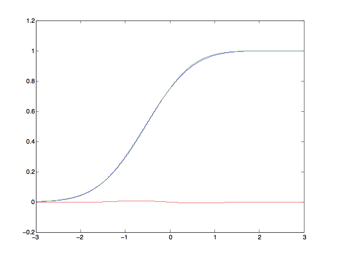
Figure 1: A numerical calculation of a distribution function under which identification fails (blue line), compared with a normal distribution function (green line).

Although no formal derivation of the counterexample is given, this result suggests the following:

• In the bivariate probit model with continuous common exogenous covariates and no excluded instruments, the parameters will be, at best, weakly identified;

• This also implies that, in the semiparametric model considered in Theorem 2.3, the structural parameters and the marginal distributions are not identified without an exclusion restriction, even if $X_{1}$ has large support.

2.3.2 No Restrictions on Dependence Structures

When the restriction imposed on $C(\cdot,\cdot)$ (i.e., Assumption 5) is completely relaxed, the underlying parameters of model (1.1) may fail to be identified, regardless of whether the exclusion restriction holds. That is, a structure describing how the unobservables $(\varepsilon,\nu)$ are dependent on each other is necessary for identification. This is closely related to the results in the literature that the treatment parameters (which are lower dimensional functions of the individual parameters) in triangular models similar to (1.1) are only partially identified without distributional assumptions; see Bhattacharya et al. (2008), Chiburis (2010), Shaikh and Vytlacil (2011), and Mourifié (2015).

Suppose Assumptions 1–4 hold. Then the model becomes a semiparametric threshold crossing model in that the joint distribution is completely unspecified. Then, as a special case of Shaikh and Vytlacil (2011), one can easily derive bounds for the ATE $F_{\varepsilon}(x^{\prime}\beta+\delta_{1})-F_{\varepsilon}(x^{\prime}\beta)$. The sharpness of these bounds is shown in their paper under a rectangular support assumption for $(X,Z)$, which is, in turn, relaxed in Mourifié (2015). In addition, using Assumption 6, one can also derive bounds for the individual parameters $x^{\prime}\beta$ and $\delta_{1}$, as shown in Chiburis (2010). When there are no excluded instruments in the model, Chiburis (2010) shows that the bounds on the ATE do not improve on the bounds of Manski (1990), whose argument applies to the individual parameters.

3 Sieve and Parametric ML Estimations

Based on the identification results, we now consider estimation. Let $\psi\equiv(\alpha^{{}^{\prime}},\beta^{{}^{\prime}},\delta_{1},\gamma,\rho)$ denote the vector of the structural individual parameters. Let $f_{\epsilon}$ and $f_{\nu}$ be the density functions associated with the distribution functions $F_{\epsilon}$ and $F_{\nu}$, respectively, of the unobservables. Then, $(\psi^{{}^{\prime}},f_{\epsilon},f_{\nu})^{{}^{\prime}}$ is the set of parameters in the semiparametric version of the model. The model becomes fully parametric, once the infinite-dimensional parameters $f_{\epsilon}$ and $f_{\nu}$ are fully characterized by some finite-dimensional parameters, i.e., $f_{\epsilon}(\cdot;\eta_{\epsilon})$ and $f_{\nu}(\cdot;\eta_{\nu})$ for $\eta_{\epsilon}\in\mathbb{R}^{d_{\eta_{\epsilon}}}$ and $\eta_{\nu}\in\mathbb{R}^{d_{\eta_{\nu}}}$. This yields $(\psi^{{}^{\prime}},\eta_{\epsilon}^{{}^{\prime}},\eta_{\nu}^{{}^{\prime}})^{{}^{\prime}}$ to be the set of parameters in the parametric version of the model. For either case, the parameter of the model is denoted as $\theta$ for convenience. That is, $\theta\equiv(\psi^{{}^{\prime}},f_{\epsilon},f_{\nu})^{{}^{\prime}}$ in the semiparametric model and $\theta\equiv(\psi^{{}^{\prime}},\eta_{\epsilon}^{{}^{\prime}},\eta_{\nu}^{{}^{\prime}})^{{}^{\prime}}$ in the parametric model. For the rest of this paper, we explicitly express $\theta_{0}$ to be the true parameter value for $\theta$. This applies to all the other parameter expressions.

Let $\tilde{\Psi}$ be the parameter space for $\psi$. For the parametric model, the spaces for the finite-dimensional parameters $\eta_{\epsilon}$ and $\eta_{\nu}$ are denoted as $\mathbf{H}_{\epsilon}\subseteq\mathbb{R}^{d_{\eta_{\epsilon}}}$ and $\mathbf{H}_{\nu}\subseteq\mathbb{R}^{d_{\eta_{\nu}}}$, respectively. Then, the parameter space $\tilde{\Theta}$ for $\theta\equiv(\psi^{{}^{\prime}},\eta_{\epsilon}^{{}^{\prime}},\eta_{\nu}^{{}^{\prime}})^{{}^{\prime}}$ becomes a Cartesian product of $\tilde{\Psi}$, $\mathbf{H}_{\epsilon}$, and $\mathbf{H}_{\nu}$, i.e., $\tilde{\Theta}\equiv\tilde{\Psi}\times\mathbf{H}_{\epsilon}\times\mathbf{H}_{\nu}\subseteq\mathbb{R}^{d_{\psi}+d_{\eta_{\epsilon}}+d_{\eta_{\nu}}}$, in the parametric model. For the semiparametric model, we consider the following function spaces as the spaces for $f_{\epsilon}$ and $f_{\nu}$:

$$\mathcal{F}_{j}\equiv\left\{f=q^{2}:q\in\mathcal{F},\int\{q(x)\}^{2}dx=1\right\},$$ (3.1)

where $j\in\{\epsilon,\nu\}$ and $\mathcal{F}$ is a space of functions, which we specify later. Then, the parameter space $\tilde{\Theta}$ of $\theta\equiv(\psi^{{}^{\prime}},f_{\epsilon},f_{\nu})^{{}^{\prime}}$ can be written as $\tilde{\Theta}\equiv\tilde{\Psi}\times\mathcal{F}_{\epsilon}\times\mathcal{F}_{\nu}$ in the semiparametric model. Note that the function spaces $\mathcal{F}_{\epsilon}$ and $\mathcal{F}_{\nu}$ contain functions that are nonnegative.

We adopt the ML method to estimate the parameters in the model. Let $\{W_{i}=\{Y_{i},D_{i},X_{i}^{{}^{\prime}},Z_{i}^{{}^{\prime}}\}:i=1,2,...,n\}$ be the random sample. For both parametric and semiparametric models with corresponding $\theta$, we define the conditional density function of $(Y_{i},D_{i})$ conditional on $(X_{i}^{{}^{\prime}},Z_{i}^{{}^{\prime}})^{{}^{\prime}}$ as

$$f(Y_{i},D_{i}|X_{i},Z_{i};\theta)={\textstyle\prod\limits_{y,d=0,1}}[p_{yd}(X_{i},Z_{i};\theta)]^{\mathbf{1}\{Y_{i}=y,D_{i}=d\}},$$

where $p_{yd}(x,z;\theta)$ abbreviates the right hand side expression that equates $p_{yd,xz}$ in (2.2). Then, the log of density $l(\theta,w)\equiv\log f(y,d|x,z;\theta)$ becomes

$$l(\theta,W_{i})\equiv{\textstyle\sum\limits_{y,d=0,1}}\mathbf{1}_{yd}(Y_{i},D_{i})\cdot\log p_{yd}(X_{i},Z_{i};\theta),$$ (3.2)

where $\mathbf{1}_{yd}(Y_{i},D_{i})\equiv\mathbf{1}\{Y_{i}=y,D_{i}=d\}$. Consequently, the log-likelihood function can be written as $Q_{n}(\theta)=\frac{1}{n}\sum\limits_{i=1}^{n}l(\theta,W_{i})$.

Now, the ML estimator $\tilde{\theta}_{n}$ of $\theta_{0}\equiv(\psi_{0}^{{}^{\prime}},\eta_{\epsilon 0},\eta_{\nu 0})^{{}^{\prime}}$ in the parametric model is defined as

$$\tilde{\theta}_{n}\equiv\arg\max_{\theta\in\tilde{\Theta}}{\textstyle Q_{n}(\theta)}.$$ (3.3)

For the semiparametric model, let $\mathcal{F}_{\varepsilon n}$ and $\mathcal{F}_{\nu n}$ be appropriate sieve spaces for $\mathcal{F}_{\varepsilon}$ and $\mathcal{F}_{\nu}$, respectively, and let $f_{\epsilon n}(\cdot;a_{\epsilon n})$ and $f_{\nu n}(\cdot;a_{\nu n})$ be the sieve approximations of $f_{\epsilon}$ and $f_{\nu}$ on their sieve spaces $\mathcal{F}_{\epsilon n}$ and $\mathcal{F}_{\nu n}$, respectively. Then, we define the sieve ML estimator $\hat{\theta}_{n}$ of $\theta_{0}\equiv(\psi_{0}^{{}^{\prime}},f_{\epsilon 0},f_{\nu 0})^{{}^{\prime}}$ in the semiparametric model as follows:

$$\hat{\theta}_{n}\equiv\arg\max_{\theta\in\tilde{\Theta}_{n}}{\textstyle Q_{n}(\theta)},$$ (3.4)

where $\tilde{\Theta}_{n}\equiv\tilde{\Psi}\times\mathcal{F}_{\epsilon n}\times\mathcal{F}_{\nu n}$ is the sieve space for $\theta$.

With the parameter spaces $\mathcal{F}_{\epsilon}$ and $\mathcal{F}_{\nu}$ in (3.1), we are interested in a class of “smooth” univariate square root density functions. Specifically, we assume that $\sqrt{f_{\epsilon}}$ and $\sqrt{f_{\nu}}$ belong to the class of p-smooth functions and we restrict our attention to linear sieve spaces for $\mathcal{F}_{\epsilon}$ and $\mathcal{F}_{\nu}$. In this case, the choice of sieve spaces for $\mathcal{F}_{\epsilon}$ and $\mathcal{F}_{\nu}$ depends on the supports of $\epsilon$ and $\nu$. If the supports are bounded, then one can use the polynomial sieve, trigonometric sieve, or cosine sieve. When the supports are unbounded, then we can use the Hermite polynomial sieve or the spline wavelet sieve.

In this paper, we implicitly assume that the copula function is correctly specified. As mentioned earlier, using a parametric copula may lead to model misspecification. It is well known that when the model is misspecified, the ML estimator converges to a pseudo-true value which minimizes the Kullback-Leibler (KL) divergence (e.g., White (1982)). This result applies to a semiparametric model (e.g., Chen and Fan (2006a) and Chen and Fan (2006b)) as in our semiparametric case. We, however, do not investigate the asymptotic properties of the sieve estimators under copula misspecification, as it is beyond the scope of this paper. Instead, later in simulation, we investigate how the copula misspecification affects the performance of estimators.

4 Asymptotic Theory for Sieve ML Estimators

In this section, we provide the asymptotic theory for the sieve ML estimator $\hat{\theta}_{n}$ of $\theta\equiv(\psi^{{}^{\prime}},f_{\epsilon},f_{\nu})^{{}^{\prime}}$ in the semiparametric model. This theory will be useful for practitioners to conduct inference. The asymptotic theory for the ML estimator $\tilde{\theta}_{n}$ of $\theta\equiv(\psi^{{}^{\prime}},\eta_{\epsilon},\eta_{\nu})^{{}^{\prime}}$ in the parametric model is relatively standard and can be found in, e.g., Newey and McFadden (1994). The theory establishes that the parametric ML estimator is consistent, asymptotically normal, and efficient under some regularity conditions. To investigate the asymptotic properties of the sieve ML estimator, we slightly modify our model as follows.

Let $G(\cdot$) be a strictly increasing function mapping from $\mathbb{R}$ to $[0,1]$. We further assume that $G$ is differentiable and that its derivative $g(x)\equiv\frac{dG(x)}{dx}$ is bounded away from zero on $\mathbb{R}$. Then, without loss of generality (e.g., Bierens (2014)), we consider the following transformation of $F_{\epsilon 0}$ and $F_{\nu 0}$ as:

$$F_{\epsilon 0}(x) =H_{\epsilon 0}(G_{\epsilon}(x)),\quad F_{\nu 0}(x)=H_{\nu 0}(G_{\nu}(x)),$$ (4.1)

where $H_{\epsilon 0}(\cdot)$ and $H_{\nu 0}(\cdot)$ are unknown distribution functions on $[0,1]$. For $G$, we can choose the standard normal distribution function or the logistic distribution function. Since we assume that the distribution functions of $\epsilon$ and $\nu$ admit density functions, we require that $H_{\epsilon 0}$ and $H_{\nu 0}(\cdot)$ be differentiable, and write their derivatives as $h_{\epsilon 0}(\cdot)$ and $h_{\nu 0}(\cdot)$, respectively. For each $j\in\{\epsilon,\nu\}$, let $\mathcal{H}_{j}\equiv\{h_{j}=q^{2}:q\in\mathcal{F}\}$ for some function space $\mathcal{F}$. With this modification, we redefine the parameter as $\theta=(\psi^{{}^{\prime}},h_{\epsilon},h_{\nu})^{{}^{\prime}}\in\tilde{\Theta}^{\dagger}\equiv\tilde{\Psi}\times\mathcal{H}_{\epsilon}\times\mathcal{H}_{\nu}$. Note that, using the transformation of the distribution functions in equation (4.1), the unknown infinite-dimensional parameters are defined on a bounded domain. In the online appendix, we show that the transformation does not affect the identification result.

We redefine the parameter space to facilitate developing the asymptotic theory. The identification requires that the space of the finite-dimensional parameter $\tilde{\Psi}$ be open and convex (see Theorems 2.2 and 2.3), and thus $\tilde{\Psi}$ cannot be compact. We introduce an “optimization space” that contains the true parameter $\psi_{0}$ and consider it as the parameter space of $\psi$. Formally, we restrict the parameter space for estimation in the following way.

Assumption 8.

There exists a compact and convex subset $\Psi\subseteq\tilde{\Psi}$ such that $\psi_{0}\in int(\Psi)$, where $int(A)$ is the interior of the set $A$.

With the optimization space, we define the parameter space as $\Theta\equiv\Psi\times\mathcal{H}_{\epsilon}\times\mathcal{H}_{\nu}$, and the corresponding sieve space is denoted by $\Theta_{n}\equiv\Psi\times\mathcal{H}_{\epsilon n}\times\mathcal{H}_{\nu n}$. Then, the sieve ML estimator in equation (3.4) is also redefined as follows:

$$\hat{\theta}_{n}\equiv\text{arg max}_{\theta\in\Theta_{n}}Q_{n}(\theta).$$ (4.2)

4.1 Consistency of the Sieve ML Estimators

We begin by showing the consistency of the sieve ML estimator. Since the parameter involves both finite- and infinite-dimensional objects, we establish the consistency of the sieve ML estimators with respect to a pseudo distance function $d_{c}$ on $\Theta\times\Theta$. All of the norms and the definitions of function spaces in this paper are provided in the online appendix.

We present the following assumptions, under which the sieve ML estimator in equation (4.2) is consistent with respect to the pseudo-metric $d_{c}(\cdot,\cdot)$.

Assumption 9.

There exists a measurable function $\underline{p}(X,Z)$ such that for all $\theta\in\Theta$ and for all $y,d=0,1$, $p_{yd,XZ}(\theta)\geq\underline{p}(X,Z)$, with $E|\log(\underline{p}(X,Z))|<\infty$ and $E\left[\frac{1}{\underline{p}(X,Z)^{2}}\right]<\infty$.

Assumption 10.

$\{W_{i}:i=1,2,...,n\}$ is a random sample, with $E\left[||(X_{i}^{{}^{\prime}},Z_{i}^{{}^{\prime}})^{{}^{\prime}}||_{E}^{2}\right]<\infty$.

Assumption 11.

(i) $\sqrt{h_{\epsilon 0}},\sqrt{h_{\nu 0}}\in\Lambda_{R}^{p}([0,1])$, with $p>\frac{1}{2}$ and some $R>0$; (ii) $\mathcal{H}_{\epsilon}=\mathcal{H}_{\nu}=\mathcal{H}$ where $\mathcal{H}\equiv\left\{h=q^{2}:q\in\Lambda_{R}^{p}([0,1]),\int_{0}^{1}q=1\right\}$, with $R$ being defined as in (i) and $\Lambda_{R}^{p}([0,1])$ being a Hölder ball with radius $R$; (iii) the density functions $h_{\epsilon 0}$ and $h_{\nu 0}$ are bounded away from zero on $[0,1]$.

Assumption 12.

(i) $\mathcal{H}_{\epsilon n}=\mathcal{H}_{\nu n}\equiv\{h\in\mathcal{H}:h(x)=p^{k_{n}}(x)^{{}^{\prime}}a_{k_{n}},a_{k_{n}}\in\mathbb{R}^{k_{n}},||h||_{\infty}<2R^{2}\}$, where $k_{n}\rightarrow\infty$ and $k_{n}/n\rightarrow 0$ as $n\rightarrow\infty$; (ii) for all $j\geq 1$, we have $\Theta_{j}\subseteq\Theta_{j+1}$, and there exists a sequence $\{\pi_{j}\theta_{0}\}_{j}$ such that $d_{c}(\pi_{j}\theta_{0},\theta_{0})\rightarrow 0$ as $j\rightarrow\infty$.

Assumption 13.

For $j=1,2$, let $C_{j}(u_{1},u_{2};\rho)\equiv\frac{\partial C(u_{1},u_{2};\rho)}{\partial u_{j}}$ and $C_{\rho}(u_{1},u_{2};\rho)\equiv\frac{\partial C(u_{1},u_{2};\rho)}{\partial\rho}$. The derivatives $C_{j}(\cdot,\cdot;\cdot)$ and $C_{\rho}(\cdot,\cdot;\cdot)$ are uniformly bounded for all $j=1,2$.

Assumption 9 guarantees that the log-likelihood function $l(\theta,W_{i})$ is well defined for all $\theta\in\Theta$ and that $Q_{0}(\theta_{0})>-\infty$. Assumption 10 restricts the data generating process (DGP), and assumes the existence of moments of the data. Assumption 11 defines the parameter space and implies that the infinite-dimensional parameters are in some smooth class called a Hölder class. Note that conditions (i) and (ii) in Assumption 11 together imply that $h_{\epsilon 0}$ and $h_{\nu 0}$ belong to $\Lambda_{\tilde{R}}^{p}([0,1])$, where $\tilde{R}\equiv 2^{m+1}R^{2}<\infty$. Thus, we may assume that $h_{\epsilon 0}$ and $h_{\nu 0}$ belong to a Hölder ball with smoothness $p$ under Assumption 11. The condition that $\mathcal{H}_{\epsilon}$ and $\mathcal{H}_{\nu}$ are the same can be relaxed, but it is imposed for simplicity. The first part of Assumption 12 restricts our choice of sieve spaces for $\mathcal{H}_{\epsilon}$ and $\mathcal{H}_{\nu}$ to linear sieve spaces with order $k_{n}$. This can be relaxed so that the choice of $k_{n}$ is different for $h_{\epsilon}$ and $h_{\nu}$. The latter part of Assumption 12 requires that the sieve space be chosen appropriately so that the unknown parameters can be well-approximated. Because the unknown infinite-dimensional parameters belong to a Hölder ball and are defined on bounded supports, we can choose the polynomial sieve, trigonometric sieve, cosine sieve, or spline sieve. For example, if we choose the polynomial sieve or the spline sieve, then one can show that $d_{c}(\pi_{k_{n}}\theta_{0},\theta_{0})=O(k_{n}^{-p})$ (e.g., Lorentz (1966)). Assumption 13 imposes the boundedness of the derivatives of the copula function.

The following theorem demonstrates that under the above assumptions, the sieve estimator $\hat{\theta}_{n}$ is consistent with respect to the pseudo metric, $d_{c}$.

Theorem 4.1.

Suppose that Assumptions 1–5 and 7 hold. If Assumptions 8–13 are satisfied, then $d_{c}(\hat{\theta}_{n},\theta_{0})\overset{p}{\rightarrow}0$.

4.2 Convergence Rates

In this section, we derive the convergence rate of the sieve ML estimator. The convergence rate provides information on how fast the estimator converges to the true parameter value. Heuristically, the faster the convergence rate, the larger the effective sample size is for estimation. The next theorem demonstrates the convergence rate of the sieve ML estimator with respect to the $L^{2}$-norm $||\cdot||_{2}$.

Theorem 4.2.

Suppose that Assumptions 1–5 and 7–13 hold. If Assumption 17 in the online appendix additionally holds, then we have $||\hat{\theta}_{n}-\theta_{0}||_{2}=O_{p}\left(\max\left\{\sqrt{k_{n}/n},k_{n}^{-p}\right\}\right)$. Furthermore, if we choose $k_{n}\propto n^{\frac{1}{2p+1}}$, then we have $||\hat{\theta}_{n}-\theta_{0}||_{2}=O_{p}\left(n^{-\frac{p}{2p+1}}\right)$.

The former convergence rate is standard in the literature, where the first term corresponds to variance, which increases in $k_{n}$, and the second term corresponds to the approximation error $||\theta_{0}-\pi_{k}\theta_{0}||_{2}$, which decreases in $k_{n}$. The choice of $k_{n}\propto n^{\frac{1}{2p+1}}$ yields the optimal convergence rate, which is slower than the parametric rate ($n^{-1/2}$). Note that this rate increases with the degree of smoothness, $p$.

4.3 Asymptotic Normality of Smooth Functionals

We now establish the asymptotic normality of smooth functionals. The parameters in our model contains both finite- and infinite-dimensional parameters, and many objects of interest are written as functionals of both types of the parameters. The results of this section can be used to calculate the standard error of the estimate of a functional of interest (including the individual finite-dimensional parameters), or to conduct inference (i.e., testing hypotheses and constructing confidence intervals) based on normal approximation.

Before proceeding, we strengthen the smoothness condition in Assumption 5. Let $C_{ij}(u_{1},u_{2};\rho)$ denote the second-order partial derivative of a copula function $C(u_{1},u_{2};\rho)$ with respect to $i$ and $j$, for $i,j\in\{u_{1},u_{2},\rho\}$.

Assumption 14.

The copula function $C(u_{1},u_{2};\rho)$ is twice continuously differentiable with respect to $u_{1},u_{2},$ and $\rho$, and its first- and second- order partial derivatives are well defined in a neighborhood of $\theta_{0}$.

Let $\mathbb{V}$ be the linear span of $\Theta-\{\theta_{0}\}$. For $t\in[0,1]$, define the directional derivative of $l(\theta,W)$ at the direction $v\in\mathbb{V}$ as

$$\left.\frac{dl(\theta_{0}+tv,W)}{dt}\right|_{t=0} \equiv\lim_{t\rightarrow 0}\frac{l(\theta_{0}+tv,W)-l(\theta_{0})}{t}=\frac{\partial l(\theta_{0},W)}{\partial\psi^{{}^{\prime}}}v_{\psi}+\sum_{j\in\{\epsilon,\nu\}}\frac{\partial l(\theta_{0},W)}{\partial h_{j}}[v_{j}],$$ (4.3)

where $\frac{\partial l(\theta_{0},W)}{\partial\psi^{{}^{\prime}}}v_{\psi}$, $\frac{\partial l(\theta_{0},W)}{\partial h_{\epsilon}}[v_{\epsilon}]$, and $\frac{\partial l(\theta_{0},W)}{\partial h_{\nu}}[v_{\nu}]$ are given by equations (B.4)–(B.6) in the online appendix. If we denote the closed linear span of $\mathbb{V}$ under the Fisher norm $||\cdot||$ by $\bar{\mathbb{V}}$, then $(\bar{\mathbb{V}},||\cdot||)$ is a Hilbert space.

Let $T:\Theta\rightarrow\mathbb{R}$ be a functional. For any $v\in\mathbb{V}$, we write

$$\frac{\partial T(\theta_{0})}{\partial\theta^{{}^{\prime}}}[v]\equiv\lim_{t\rightarrow 0}\frac{T(\theta_{0}+tv)-T(\theta_{0})}{t},$$

provided the right hand side limit is well defined. The following assumption characterizes the smoothness of the functional $T$.

Assumption 15.

The following conditions hold:

(i) there exist constants $w>1+\frac{1}{2p}$ and a small $\epsilon_{0}>0$ such that for any $v\in\mathbb{V}$ with $||v||\leq\epsilon_{0}$,

$$\left|T(\theta_{0}+v)-T(\theta_{0})-\frac{\partial T(\theta_{0})}{\partial\theta^{{}^{\prime}}}[v]\right|=O(||v||^{w});$$

(ii) For any $v\in\mathbb{V}$, $T(\theta_{0}+tv)$ is continuously differentiable in $t\in[0,1]$ around $t=0$, and

$$\left\|\frac{\partial T(\theta_{0})}{\partial\theta^{{}^{\prime}}}\right\|\equiv\sup_{v\in\mathbb{V},||v||>0}\frac{\left|\frac{\partial T(\theta_{0})}{\partial\theta^{{}^{\prime}}}[v]\right|}{||v||}<\infty.$$

Assumption 15 defines a smooth functional $T$ and guarantees the existence of $v^{*}\in\bar{\mathbb{V}}$ such that $<v^{*},v>=\frac{\partial T(\theta_{0})}{\partial\theta^{{}^{\prime}}}[v]$ for all $v\in\mathbb{V}$ and $||v^{*}||^{2}=\left\|\frac{\partial T(\theta_{0})}{\partial\theta^{{}^{\prime}}}\right\|^{2}$. Here, we call $v^{*}$ the Riesz representer for the functional $T$.

The next assumption requires that the Riesz representer be well approximated over the sieve space and that it converges at a rate with respect to the Fisher norm.

Assumption 16.

There exists $\pi_{n}v^{*}\in\Theta_{n}-\{\theta_{0}\}$ such that $||\pi_{n}v^{*}-v^{*}||=o(n^{-1/4})$.

The following proposition states that the plug-in sieve ML estimator $T(\hat{\theta}_{n})$ of $T(\theta_{0})$ is $\sqrt{n}$-asymptotically normally distributed under certain conditions. The technical conditions (Assumptions 17, 18 and 19) can be found in the online appendix.

Proposition 4.1.

Suppose that Assumptions 1–5, 7–16, 17–19 are satisfied. If $k_{n}\propto n^{\frac{1}{2p+1}}$, then we have

$$\sqrt{n}(T(\hat{\theta}_{n})-T(\theta_{0}))\overset{d}{\rightarrow}\mathcal{N}\left(0,\left\|\frac{\partial T(\theta_{0})}{\partial\theta^{{}^{\prime}}}\right\|^{2}\right).$$

It is worth noting that, although the parameter $T(\theta_{0})$ contains an infinite-dimensional object (i.e., the marginal distributions of $\epsilon$ and $\nu$), the sieve plug-in estimator is $\sqrt{n}$-estimable due to the fact that $T$ is a smooth functional.

4.3.1 Example 1: Asymptotic Normality for the Finite-Dimensional Parameter $\psi_{0}$

The finite-dimensional parameter $\psi_{0}$ is a special case of the smooth functionals. Here, we demonstrate the asymptotic normality of the sieve estimator of the finite-dimensional parameter $\psi_{0}$.

Theorem 4.3.

Suppose that Assumptions 1–5, 7–14, 16, 17–20 hold. Then, we have

$$\sqrt{n}(\hat{\psi}_{n}-\psi_{0})\overset{d}{\rightarrow}\mathcal{N}\left(0,\mathcal{I}_{*}(\psi_{0})^{-1}\right),$$ (4.4)

and the form of $\mathcal{I}_{*}(\psi)$ is given in the online appendix.

The covariance matrix in (4.4) needs to be estimated. To do so, CFT06 adopt the covariance estimation method proposed by Ai and Chen (2003). Since an infinite-dimensional optimization is involved in calculating $\mathcal{S}_{\psi_{0}}$, we provide a sieve estimator of $\mathcal{I}_{*}(\psi_{0})^{-1}$. The sieve spaces for $b_{\epsilon}$ and $b_{\nu}$ can be the same as those for $h_{\epsilon}$ and $h_{\nu}$, respectively. As in Ai and Chen (2003), we first estimate efficient score functions by solving the following minimization problem: for all $k=1,2,...,d_{\psi}$,

$$(\hat{b}_{\epsilon k},\hat{b}_{\nu k})\equiv\arg\min_{(b_{\epsilon k},b_{\nu k})\in\mathcal{H}_{\epsilon n}\times\mathcal{H}_{\nu n}}\frac{1}{n}\sum_{i=1}^{n}\left\{\frac{\partial l(\hat{\theta}_{n},W_{i})}{\partial\psi_{k}}-\left(\frac{\partial l(\hat{\theta}_{n},W_{i})}{\partial h_{\epsilon}}[b_{\epsilon k}]+\frac{\partial l(\hat{\theta}_{n},W_{i})}{\partial h_{\nu}}[b_{\nu k}]\right)\right\}^{2}.$$

Let $\hat{b}_{j}=(\hat{b}_{j1},\hat{b}_{j2},...,\hat{b}_{jd_{\psi}})^{{}^{\prime}}$ for given $j\in\{\epsilon,\nu\}$ and compute

$$\hat{\mathcal{I}}_{*}(\hat{\psi}_{n})= \frac{1}{n}\sum_{i=1}^{n}\left\{\left[\frac{\partial l(\hat{\theta}_{n},W_{i})}{\partial\psi}-\left(\frac{\partial l(\hat{\theta}_{n},W_{i})}{\partial h_{\epsilon}}[\hat{b}_{\epsilon}]+\frac{\partial l(\hat{\theta}_{n},W_{i})}{\partial h_{\nu}}[\hat{b}_{\nu}]\right)\right]\right.$$

$$\times\left.\left[\frac{\partial l(\hat{\theta}_{n},W_{i})}{\partial\psi}-\left(\frac{\partial l(\hat{\theta}_{n},W_{i})}{\partial h_{\epsilon}}[\hat{b}_{\epsilon}]+\frac{\partial l(\hat{\theta}_{n},W_{i})}{\partial h_{\nu}}[\hat{b}_{\nu}]\right)\right]^{{}^{\prime}}\right\}$$

to obtain a consistent estimator of $\mathcal{I}_{*}(\psi_{0})$. We now summarize this result as follows:

Theorem 4.4.

Suppose that assumptions in Theorem 4.3 hold. Then, $\hat{\mathcal{I}}_{*}(\hat{\psi}_{n})=\mathcal{I}_{*}(\psi_{0})+o_{p}(1)$.

The proof of the theorem can be found in Theorem 5.1 in Ai and Chen (2003).

4.3.2 Example 2: Asymptotic Normality for the Conditional ATE

We now consider the conditional ATE, $E[Y_{1}-Y_{0}|X=x]=F_{\epsilon 0}(x^{{}^{\prime}}\beta_{0}+\delta_{10})-F_{\epsilon 0}(x^{{}^{\prime}}\beta_{0})$. From Proposition 4.1, we provide the asymptotic normality of the sieve plug-in estimator of the conditional ATE:

Theorem 4.5.

Let $x\in\text{supp}(X)$ be given. Suppose that the conditions in Proposition 4.1 hold with $T(\theta_{0})=ATE(\theta_{0};x)$. Then, we have

$$\sqrt{n}(ATE(\hat{\theta}_{n};x)-ATE(\theta_{0};x))\overset{d}{\rightarrow}\mathcal{N}\left(0,\left\|\frac{\partial ATE(\theta_{0};x)}{\partial\theta^{{}^{\prime}}}[v]\right\|^{2}\right),$$ (4.5)

where $\left\|\frac{\partial ATE(\theta_{0};x)}{\partial\theta^{{}^{\prime}}}[v]\right\|^{2}=\sup_{v\in\mathbb{V},||v||>0}\frac{\left|\frac{\partial ATE(\theta_{0};x)}{\partial\theta^{{}^{\prime}}}[v]\right|}{||v||}$, and the form of $\frac{\partial ATE(\theta_{0};x)}{\partial\theta^{{}^{\prime}}}[v]$ is given by (B.7) in the online appendix.

Furthermore, the asymptotic variance in (4.5) can be estimated as follows:

$$\hat{\sigma}_{ATE(\theta;x)}^{2}\equiv\max_{v\in\Theta_{n}}\left\|\frac{\partial ATE(\hat{\theta}_{n};x)}{\partial\theta^{{}^{\prime}}}[v]\right\|^{2}.$$

4.4 Weighted Bootstrap

The asymptotic variances characterized in the previous subsection can be estimated using the sieve methods. In practice, estimating asymptotic variances may be sensitive to the choice of the number of sieve approximation terms. Furthermore, when the dimension of $\theta_{0}$ is large, it is relatively cumbersome to estimate the asymptotic variance of the sieve estimator for the finite-dimensional parameter. In this subsection, we briefly discuss the weighted bootstrap as an alternative procedure.

For general semiparametric M-estimation, Ma and Kosorok (2005) and Cheng and Huang (2010) provide the validity of the weighted bootstrap for finite-dimensional parameters in a class of semiparametric models that includes our model. Related to these results, Chen and Pouzo (2009) provide the bootstrap validity in semiparametric conditional moment models. We do not pursue to prove the bootstrap validity in this paper, as these references sufficiently address it. In our empirical exercise, we use the weighted bootstrap scheme proposed in these papers to obtain the standard errors of the estimated functionals of interest. Let $T(\theta_{0})$ be a smooth functional of interest and $B$ be the number of bootstrap iterations. The weighted bootstrap is carried out as follows:

1. For each $b=1,2,...,B$, let $\{B_{i}^{(b)}:i=1,2,...,n\}$ be a random sample generated from a positive random variable $B_{i}$ such that $EB_{i}=1$, $Var(B_{i})=1$, and is independent of $\{W_{i}:i=1,2,...n\}$.

2. For each bootstrap iteration $b=1,2,...,B$, define $\hat{\theta}_{n}^{*(b)}$ be a bootstrap estimate of $\theta_{0}$:

   $$\hat{\theta}_{n}^{*(b)}\equiv\arg\max_{\theta\in\tilde{\Theta}_{n}}{\textstyle Q_{n}^{*(b)}(\theta)},$$

   where $Q_{n}^{*(b)}(\theta)\equiv\frac{1}{n}\sum\limits_{i=1}^{n}B_{i}^{(b)}\cdot l(\theta,W_{i})$. Obtain the bootstrap estimate of the functional of interest by using $\hat{\theta}_{n}^{*(b)}$ and denote it by $T(\hat{\theta}_{n}^{*(b)})$.

3. The bootstrap standard error of $T(\hat{\theta}_{n})$ is given by $\sqrt{\frac{1}{B}\sum_{b=1}^{B}\left(T(\hat{\theta}_{n}^{*(b)})-\bar{T}_{B}^{*}\right)}$, where $\bar{T}_{B}^{*}\equiv\frac{1}{B}\sum_{b=1}^{B}T(\hat{\theta}_{n}^{*(b)})$.

One may use the bootstrap standard errors to construct confidence intervals, and such confidence intervals rely on the normal approximation. As an alternative to the normal approximation, one can use percentile confidence intervals. For a small $p\in(0,1)$, a $(1-p)\times 100$ percent percentile confidence interval for a functional $T(\theta_{0})$ is constructed as follows:

$$PCI(p)\equiv\left[Q_{T}^{*}(p/2),\quad Q_{T}^{*}(1-p/2)\right],$$

where $Q_{T}^{*}(\tau)$ is the $\tau$-th quantile of bootstrap estimates $\{T(\hat{\theta}_{n}^{*(b)}):b=1,2,...,B\}$. We suggest that practitioners use the percentile confidence intervals rather than the confidence intervals with the bootstrap standard errors.

5 Monte Carlo Simulation and Sensitivity Analysis

In this section, we conduct a sensitivity analysis via Monte Carlo simulation exercises to provide guidance for empirical researchers. To this end, we investigate the finite sample performance of the sieve ML estimators of the finite-dimensional parameter $\psi_{0}$ and the ATE. We compare them with the performance of the parametric ML estimators under various DGPs and model specifications, and illustrate how the parametric estimators of $\psi_{0}$ and the ATE suffer from misspecification of the marginal distribution of $\epsilon$. Note that the ATE involves $\psi_{0}$ and the marginal of $\epsilon$.

5.1 Simulation Design

We compare the performance of the parametric and semiparametric estimators when the marginal distributions are misspecified in the parametric models. To calculate the parametric estimators, we specify the parametric models with normal distributions for the marginals of $\epsilon$ and $\nu$, owing to their popularity. For the DGPs, we consider two marginals of $\epsilon$ and $\nu$: the standard normal distribution (to reflect correct specification) and a mixture of normal distributions (to reflect misspecification).

The DGPs are as follows:

$$Y_{i} =\mathbf{1}\{X_{i}\beta+D_{i}\delta_{1}\geq\epsilon\},\quad D_{i}=\mathbf{1}\{X_{i}\alpha+Z_{i}\gamma\geq\nu\},$$

where $(\alpha,\gamma,\beta,\delta_{1})=(-1,0.8,-1,1.1)$, $(X,Z)^{\prime}\sim\mathcal{N}\left((0,0)^{\prime},\begin{pmatrix}1&-0.1\\ -0.1&1\end{pmatrix}\right)$, and $(\epsilon,\nu)^{{}^{\prime}}\sim C(F_{\epsilon 0}(\cdot),F_{\nu 0}(\cdot);\rho)$. Here, $F_{\epsilon 0}$ and $F_{\nu 0}$ are normal or a mixture of normal. For $C(\cdot,\cdot;\rho)$, we consider the Gaussian, Frank, Clayton, and Gumbel copulas, which satisfy the identifying assumption (Assumption 5). The dependence structure between $\epsilon$ and $\nu$ is characterized by a one-dimensional parameter $\rho$ in all copulas considered, but the interpretation of the dependence parameter differs across the copulas. To resolve this issue, we report the Spearman’s $\rho$ corresponding to the estimated dependence parameter in each copula specification. We estimate the models with several values of $\rho$ to examine whether the performance of the estimators varies with the degree of dependence. Although we assume that the copula is correctly specified, economic theory does not provide a justification for the choice of copula. In this simulation study, we also examine the effect of copula misspecification on the performance of the estimators.

We impose a restriction that $X$ has no constant for the location normalization, and fix $\alpha$ and $\beta$ to -1 for the scale normalization. We use these normalizations in both parametric and semiparametric models, and it allows us to easily compare the performance of the parametric and semiparametric estimators. We consider two sample sizes, 500 and 1000, and all results are obtained from 2000 Monte Carlo replications. As a performance measure of the estimators, we consider the root mean squared errors (RMSEs) in our simulation.

5.2 Estimation of Parametric and Semiparametric Models

The parametric models can be estimated by the standard ML method. Since bivariate probit models are commonly used in practice, we specify the model using the Gaussian copula and normal marginals. In addition to that, we also try different copulas and normal marginals.

Consider semiparametric models. Recall that we assume that $\sqrt{h_{j}}\in\Lambda^{p}([0,1])$. Therefore, for each $j\in\{\epsilon,\nu\}$, we approximate $h_{j}$ to

$$h_{j}(x)=\frac{\left(\sum_{k=0}^{k_{nj}}a_{jk}\psi_{jk}(x)\right)^{2}}{\int_{0}^{1}\left(\sum_{k=0}^{k_{nj}}a_{jk}\psi_{jk}(x)\right)^{2}dx},$$ (5.1)

where $\{\psi_{jk}(\cdot)\}_{k=0}^{k_{nj}}$ is the set of approximating functions for $h_{j}(\cdot)$, and $k_{nj}$ is the number of approximating functions. The approximation in (5.1) guarantees that $\int_{0}^{1}h_{j}(x)dx=1$ by construction. We take the space of the polynomials as the sieve space for $h_{\epsilon}$ and $h_{\nu}$. The orders of the polynomials ($k_{n\epsilon}$ and $k_{n\nu}$) are set to be proportional to $n^{1/7}$. To incorporate the specification given in (4.1), we choose the standard normal distribution function for $G$.

5.3 Simulation Results

We begin by examining the simulation results under correct specification (i.e., the true marginal distributions and the specified marginal distributions are both normal). Table 1 shows the simulation results for $n=500$. We find that the ML estimators of $\psi$ and the ATE perform well in the parametric models, with negligible biases and small variances. The performance of the sieve ML estimators of $\psi$ and the ATE in the semiparametric models is as good as that in the parametric models, even with this moderate sample size.

Now, we consider the cases where the marginal distributions are misspecified in the parametric models. Table 2 considers the case where the true marginal distributions are a mixture of normal distributions, but the researcher specifies them as normal distributions. In this table, the RMSEs of the parametric ML estimators are larger than those of the sieve ML estimators. This implies that the parametric ML estimators suffer from misspecification while the sieve ML estimators do not. Moreover, the parametric estimators of the ATE are substantially distorted under this misspecification, presumably because the ATE is a function of the misspecified distribution of $\epsilon$. Note that the poor performance of the parametric estimators is attributed not only to large bias, but also large variance. For instance, the bias of the parametric estimator of the ATE with the Gaussian copula is 0.1377, which is about eight times larger than that of the corresponding sieve estimator. These biases of the parametric estimators of the ATE are substantial in that they do not disappear with the increased sample size. Therefore, the simulation results demonstrate that when the marginal distributions are misspecified, the sieve estimators outperform the parametric estimators in terms of the RMSE. The online appendix also contains simulation results for the cases where both the copula and the marginal distributions are misspecified. The results show that, even under copula misspecification, the sieve ML estimators remain to outperform the parametric counterparts when the marginal distributions are misspecified.

Overall, the simulation results suggest that researchers are recommended to use the semiparametric models and the sieve ML estimation proposed in this paper when they are concerned about model misspecification. The following is the summary of the main findings from our simulation study:

• When the model is correctly specified, the performance of the sieve ML estimators is comparable to that of the parametric ML estimators.

• When the marginal distributions are misspecified, the sieve ML estimation is recommended in order to improve the performance.

• The semiparametric ML estimators performs better than the parametric ML estimators under both copula and marginal misspecification. Therefore, the semiparametric models are preferred to the parametric models in such cases.

• Especially for the ATE, whenever the marginal distributions are misspecified, the parametric ML estimates can be significantly distorted.

We provide additional simulation results in the online appendix, where we consider (a) a larger sample size, (b) both copula and marginal misspecification, (c) different degrees of dependence, (d) marginal density functions of heavy tails, and (e) the coverage probabilities of bootstrap confidence intervals. Here is the summary. Across various simulation designs ((a)–(c)), our main findings remain the same. When the marginal distributions are believed to have fat tails, we recommend practitioners to use the transformation function $G$ that has fat tails. Lastly, the percentile bootstrap works well with the coverage probabilities close to its nominal level.

6 Empirical Example

In this section, we illustrate in an application the practical relevance of the theoretical results developed in this paper. It is widely recognized that health insurance coverage can be an important factor for patients’ decisions for making medical visits. At the same time, having insurances is endogenously determined by individual’s health status and socioeconomic characteristics. In our empirical application, we analyze how health insurance coverage affects an individual’s decision to visit a doctor. In this example, $Y$ is a binary outcome variable indicating whether an individual visited a doctor’s office, and $D$ is the endogenous treatment variable that indicates whether an individual has her own private insurance.

We use the 2010 wave of the Medical Expenditure Panel Survey (MEPS) as our main data source. We focus on all the visits happened in January, 2010. We restrict the sample to contain individuals with age between 25 and 64, and exclude individuals who have retained any kinds of federal or state insurance in 2010. For $Z$, we consider two instrumental variables that are used in Zimmer (2018)—the number of employees in the firm at which the individual works and a dummy variable that indicates whether a firm has multiple locations. These variables reflect how big the firm is, and the underlying rationale for using these variables as instruments is as follows: the bigger the firm is, the more likely it provides fringe benefits including health insurance. Therefore, it is likely that these instruments affect insurance status. We can argue, however, that they do not have direct effects on decisions to visit doctors. We assume that these variables are exogenous conditional on covariates. For additional covariates $W$, we include age, gender, years of education, family size (the number of family members), income, region, race, marital status, subjective physical and mental health status evaluations, and whether living in a metropolitan statistical area. For the exogenous variable $X$ in our model, we use information about the provision of paid sick leave, which is separately collected from the National Compensation Survey published by the U.S. Bureau of Labor Statistics. We match the information for various industries with the primary dataset we use. Conditional on the covariates listed above, we assume that the number of sick leave days and leave benefits are exogenous, by the same argument as for the instruments. Since $X$ and $Z$ are assumed to be exogenous only conditional on $W$, we rely on Assumption 1^′ instead of Assumption 1 for identification.

Since we include various control variables, one may concern that the resulting estimators are imprecise with a moderate sample size. It is worth emphasizing, however, that our semiparametric estimators do not suffer from the curse of dimensionality as theoretically shown in Section 4. This is because of the parametric index structure in our model. Moreover, we do not attempt to estimate the distributions of the unobservables conditional on these covariates, but only estimate the marginal distributions.

Table 3 summarizes the variables used in estimation and shows their summary statistics. While $65.7\%$ of individuals had private health insurances in January 2010, only $18.2\%$ of them visited doctors during the period. We use two variables for the pay sick leave provision (i.e., $X$)—within each industry, the percentage of workers who are provided with paid sick leave benefits and the percentage of workers who are provided with a fixed number of days for sick leave per year. The summary statistics for these two variables show that there are sufficient variations across individuals in different industries. Note that all the continuous variables are standardized in order to ensure stability in estimation.

Before estimating the parametric and semiparametric models, we run a first-stage OLS regression of $D$ on $X$, $W$, and $Z$ to see if the excluded instruments are weak. The $F$-statistic value is $167.19$, and thus we assume that the instruments are strong. For the normalization of the parametric model, we you the convention—$E[\epsilon]=E[\nu]=0$ and $Var(\epsilon)=Var(\nu)=1$. On the other hand, for the semiparametric model, we impose the normalization used in our simulation studies—i.e. we exclude the constant terms and the coefficients on $sick34$ are fixed to be corresponding parametric estimates. We choose the Gaussian copula to capture the dependence structure between $\epsilon$ and $\nu$. In both models, the standard errors are obtained by the bootstrap procedure (Section 4.4), where the bootstrap weights are generated from the exponential distribution with the parameter value $1$.

Tables 4 and 5 present the estimation results for the selection equation and the outcome equation, respectively. Between the parametric and semiparametric models, the magnitude and significance of the estimates differs, although, overall, the signs of the estimates are similar. Table 6 shows the ATE estimates evaluated at various values of $X$, as well as the estimates of the copula parameter $\rho$. The parametric estimate of $\rho$ is statistically significant under $5\%$ level, whereas the semiparametric estimate is not. We can find that the parametric estimates of the ATE are different from the corresponding semiparametric estimates. For example, the parametric ATE estimate evaluated at the $50\%$ quantile of $X$ is about $0.129$, which means that having private insurance increases the probability of visiting doctors by $12.9\%$. On the other hand, the corresponding semiparametric estimate shows that the effect is $10.4\%$. The discrepancy in the ATE estimates between the parametric and semiparametric models suggests the possible misspecification of the marginals, which is consistent with the premise of this paper.

7 Conclusions

In this paper, we propose semiparametric estimation and inference methods for generalized bivariate probit models. Specifically, we develop the asymptotic theory for the sieve ML estimators of semiparametric copula-based triangular systems with binary endogenous variables. We show that the sieve ML estimators are consistent and that their smooth functionals are $\sqrt{n}$-asymptotically normal under some regularity conditions. This semiparametric estimation approach allows for flexibility in the models and thus provides robustness in estimation and inference.

We conduct a sensitivity analysis to examine how sensitive the estimation results are to model specifications. The results show that, overall, the semiparametric sieve ML estimators perform well in terms of both bias and variance. When the marginal distributions are misspecified, the sieve ML estimators substantially outperform the parametric ML estimators and the latter exhibit substantial bias. In particular, we find that the parametric estimates of the parameters involving the misspecified marginal distributions, such as the ATE, are highly misleading. When the model is correctly specified, we find that the performance of the sieve ML estimators is comparable to that of the parametric ones. When the copula is also misspecified, the distortion of the parametric estimates under misspecification of the marginals can become even more severe, whereas the semiparametric estimates do not seem to be affected by this misspecification as long as the copula of the true DGP is within the stochastic ordering class. A related and interesting question is how the results would change if the data are not generated from this class of copulas.

We also formally show that the exclusion restriction is not only sufficient, but is also necessary for identification. Without the exclusion restriction, the model parameters are not identified or, under the normality assumption, are, at best, weakly identified. Some empirical studies ignore the exclusion restriction when estimating the model, and our non-identification result provides a caveat for practitioners.

Table 1: Correct Specification ($n=500$) (True marginal: normal)

Parametric Estimation, Gaussian Copula					Semiparametric Estimation, Gaussian Copula
	$\gamma$	$\delta_{1}$	$\rho_{sp}$	$ATE$		$\gamma$	$\delta_{1}$	$\rho_{sp}$	$ATE$
True Values	0.8000	1.1000	0.5000	0.3643	True Values	0.8000	1.1000	0.5000	0.3643
Estimate	0.8074	1.1469	0.4956	0.3657	Estimate	0.8070	1.1577	0.5037	0.3584
S.D	0.0934	0.3954	0.1537	0.0897	S.D	0.0940	0.4141	0.1528	0.0935
Bias	0.0074	0.0469	-0.0044	0.0014	Bias	0.0070	0.0577	0.0038	-0.0060
RMSE	0.0936	0.3982	0.1537	0.0897	RMSE	0.0943	0.4181	0.1528	0.0937
Parametric Estimation, Frank Copula					Semiparametric Estimation, Frank Copula
	$\gamma$	$\delta_{1}$	$\rho_{sp}$	$ATE$		$\gamma$	$\delta_{1}$	$\rho_{sp}$	$ATE$
True Values	0.8000	1.1000	0.5000	0.3643	True Values	0.8000	1.1000	0.5000	0.3643
Estimate	0.8027	1.1450	0.4909	0.3681	Estimate	0.8028	1.1556	0.4981	0.3598
S.D	0.0936	0.3379	0.1310	0.0781	S.D	0.0943	0.3588	0.1314	0.0829
Bias	0.0027	0.0450	-0.0091	0.0037	Bias	0.0028	0.0556	-0.0019	-0.0045
RMSE	0.0936	0.3409	0.1313	0.0781	RMSE	0.0944	0.3631	0.1314	0.0830
Parametric Estimation, Clayton Copula					Semiparametric Estimation, Clayton Copula
	$\gamma$	$\delta_{1}$	$\rho_{sp}$	$ATE$		$\gamma$	$\delta_{1}$	$\rho_{sp}$	$ATE$
True Values	0.8000	1.1000	0.5000	0.3643	True Values	0.8000	1.1000	0.5000	0.3643
Estimate	0.8024	1.1083	0.5075	0.3598	Estimate	0.8027	1.1275	0.5140	0.3504
S.D	0.0942	0.3371	0.1368	0.0791	S.D	0.0935	0.3719	0.1354	0.0816
Bias	0.0024	0.0083	0.0075	-0.0045	Bias	0.0027	0.0275	0.0139	-0.0139
RMSE	0.0942	0.3372	0.1370	0.0792	RMSE	0.0936	0.3729	0.1361	0.0828
Parametric Estimation, Gumbel Copula					Semiparametric Estimation, Gumbel Copula
	$\gamma$	$\delta_{1}$	$\rho_{sp}$	$ATE$		$\gamma$	$\delta_{1}$	$\rho_{sp}$	$ATE$
True Values	0.8000	1.1000	0.5000	0.3643	True Values	0.8000	1.1000	0.5000	0.3643
Estimate	0.8026	1.1339	0.5060	0.3605	Estimate	0.8035	1.1564	0.5102	0.3562
S.D	0.0974	0.4002	0.1488	0.0894	S.D	0.0994	0.4300	0.1535	0.0978
Bias	0.0026	0.0339	0.0060	-0.0038	Bias	0.0035	0.0564	0.0102	-0.0081
RMSE	0.0974	0.4016	0.1489	0.0895	RMSE	0.0995	0.4337	0.1539	0.0981

Table 2: Misspecification of Marginals ($n=500$) (True marginal: mixture of normals)

Parametric Estimation, Gaussian Copula					Semiparametric Estimation, Gaussian Copula
	$\gamma$	$\delta_{1}$	$\rho_{sp}$	$ATE$		$\gamma$	$\delta_{1}$	$\rho_{sp}$	$ATE$
True Values	0.8000	1.1000	0.5000	0.1066	True Values	0.8000	1.1000	0.5000	0.1066
Estimate	0.7994	1.0925	0.4496	0.2443	Estimate	0.8562	1.2696	0.4895	0.1241
S.D	0.1281	0.6285	0.1651	0.1129	S.D	0.1113	0.3728	0.1059	0.0653
Bias	-0.0006	-0.0075	-0.0504	0.1377	Bias	0.0562	0.1696	-0.0105	0.0174
RMSE	0.1281	0.6285	0.1726	0.1780	RMSE	0.1247	0.4096	0.1064	0.0675
Parametric Estimation, Frank Copula					Semiparametric Estimation, Frank Copula
	$\gamma$	$\delta_{1}$	$\rho_{sp}$	$ATE$		$\gamma$	$\delta_{1}$	$\rho_{sp}$	$ATE$
True Values	0.8000	1.1000	0.5000	0.1066	True Values	0.8000	1.1000	0.5000	0.1066
Estimate	0.8056	1.3088	0.3976	0.2894	Estimate	0.8377	1.2541	0.4829	0.1276
S.D	0.1272	0.5093	0.1221	0.0883	S.D	0.1141	0.3564	0.0963	0.0689
Bias	0.0056	0.2088	-0.1024	0.1827	Bias	0.0377	0.1541	-0.0171	0.0210
RMSE	0.1273	0.5504	0.1594	0.2030	RMSE	0.1202	0.3883	0.0978	0.0720
Parametric Estimation, Clayton Copula					Semiparametric Estimation, Clayton Copula
	$\gamma$	$\delta_{1}$	$\rho_{sp}$	$ATE$		$\gamma$	$\delta_{1}$	$\rho_{sp}$	$ATE$
True Values	0.8000	1.1000	0.5000	0.1066	True Values	0.8000	1.1000	0.5000	0.1066
Estimate	0.8099	1.1439	0.4236	0.2555	Estimate	0.8441	1.2234	0.4948	0.1192
S.D	0.1309	0.5236	0.1412	0.0913	S.D	0.1134	0.3611	0.0999	0.0611
Bias	0.0099	0.0439	-0.0764	0.1488	Bias	0.0441	0.1234	-0.0053	0.0126
RMSE	0.1312	0.5254	0.1605	0.1746	RMSE	0.1217	0.3816	0.1001	0.0624
Parametric Estimation, Gumbel Copula					Semiparametric Estimation, Gumbel Copula
	$\gamma$	$\delta_{1}$	$\rho_{sp}$	$ATE$		$\gamma$	$\delta_{1}$	$\rho_{sp}$	$ATE$
True Values	0.8000	1.1000	0.5000	0.1066	True Values	0.8000	1.1000	0.5000	0.1066
Estimate	0.7892	1.0326	0.4650	0.2373	Estimate	0.8484	1.2692	0.4900	0.1259
S.D	0.1333	0.5297	0.1338	0.0986	S.D	0.1142	0.3646	0.0986	0.0645
Bias	-0.0108	-0.0674	-0.0350	0.1307	Bias	0.0484	0.1692	-0.0099	0.0193
RMSE	0.1337	0.5340	0.1383	0.1637	RMSE	0.1241	0.4019	0.0991	0.0673

Table 3: Summary Statistics

	Variable	Mean	S.D	Min	Max
$Y$	Whether or not visit doctors	0.182	0.386	0	1
$D$	Whether or not have insurance	0.657	0.475	0	1
$W$	Age	42.591	10.574	25	64
	Years of education	13.433	2.892	0	17
	Income (hourly)	20.094	11.990	0.4	73.08
	Family size	2.932	1.595	1	14
	Living in MSA	0.868	0.338	0	1
	Male	0.500	0.500	0	1
	Region: NorthEast	0.141	0.348	0	1
	Region: MidWest	0.226	0.418	0	1
	Region: South	0.369	0.483	0	1
	Region: West	0.264	0.441	0	1
	Race: White	0.739	0.439	0	1
	Race: Black	0.170	0.376	0	1
	Race: Minority	0.010	0.099	0	1
	Race: Asian	0.081	0.273	0	1
	Ever married	0.782	0.413	0	1
	Physical health below Good$\dagger$	0.095	0.293	0	1
	Mental health below Good$\dagger$	0.036	0.186	0	1
$Z$	Number of employees	149.385	182.662	1	500
	Firm has multiple locations	0.682	0.466	0	1
$X$	sick 32	68.317	17.402	42	91
	sick 34	70.463	3.633	67	77
Number of observations = 7,555

$\dagger$: The original variables for these variables are coded into 5 groups - Excellent, Very Good, Good, Fair, and Poor. These variables show how much portion of individuals in the sample considers their physical/mental health is below Good (i.e. Fair or Poor).

Table 4: Estimates in Selection Equation

	Parametric	Semiparametric
age$\dagger$	0.130***	0.077***
	(0.018)	(0.038)
years of education$\dagger$	0.190***	0.098**
	(0.018)	(0.044)
family size$\dagger$	-0.120***	-0.041*
	(0.017)	(0.023)
income$\dagger$	0.268***	0.416***
	(0.028)	(0.089)
male	0.193***	0.062
	(0.036)	(0.039)
Living in MSA	-0.090*	-0.040
	(0.047)	(0.056)
Ever married	-0.112***	-0.048
	(0.043)	(0.050)
Physical health very good	0.001	-0.024
	(0.050)	(0.042)
Physical health good	0.009	-0.011
	(0.053)	(0.043)
Physical health fair	-0.097	-0.066
	(0.071)	(0.060)
Physical health poor	0.080	0.039
	(0.155)	(0.126)
Mental health very good	0.004	-0.016
	(0.043)	(0.043)
Mental health good	-0.031	-0.029
	(0.049)	(0.038)
Mental health fair	-0.009	-0.041
	(0.095)	(0.067)
Mental health poor	0.135	0.113
	(0.287)	(0.399)
Days for sick leave$\dagger$ (T32)	0.119***	0.094***
	(0.020)	(0.025)
Days for sick leave$\dagger$ (T34)	0.113***	0.113
	(0.019)	(N/A)
Number of employees $(Z_{1})$	0.228***	0.231**
	(0.020)	(0.116)
Firm has multiple locations $(Z_{2})$	0.374***	0.173***
	(0.034)	(0.067)
Region and Race Dummies	Yes	Yes
Number of Observations	7,555	7,555
Standard errors in parentheses, * $p<0.10$, ** $p<0.05$, *** $p<0.01$.

• $\dagger$ indicates that the variable is standardized.

• The coefficient on T34 in the semiparametric model is fixed for normalization.

• Gaussian copula is used.

Table 5: Estimates in Outcome Equation

	Parametric	Semiparametric
Treatment ($\delta$)	0.493***	0.368**
	(0.168)	(0.183)
age$\dagger$	0.055***	0.059
	(0.020)	(0.047)
years of education$\dagger$	0.142***	0.126*
	(0.028)	(0.066)
family size$\dagger$	-0.055***	-0.052*
	(0.021)	(0.030)
income$\dagger$	0.018	0.031
	(0.026)	(0.068)
male	-0.398***	-0.373**
	(0.037)	(0.169)
Living in MSA	0.063	0.040
	(0.052)	(0.061)
Ever married	0.188***	0.179**
	(0.049)	(0.084)
Physical health very good	0.227***	0.201**
	(0.056)	(0.084)
Physical health good	0.395***	0.356***
	(0.059)	(0.130)
Physical health fair	0.691***	0.644***
	(0.077)	(0.224)
Physical health poor	0.978***	0.959*
	(0.163)	(0.492)
Mental health very good	-0.033	-0.040
	(0.048)	(0.057)
Mental health good	-0.066	-0.064
	(0.053)	(0.064)
Mental health fair	0.042	0.053
	(0.105)	(0.154)
Mental health poor	0.300	0.186
	(0.297)	(0.320)
Days for sick leave$\dagger$ (T32)	-0.026	-0.023
	(0.026)	(0.027)
Days for sick leave$\dagger$ (T34)	-0.049**	-0.049
	(0.025)	(N/A)
Region and Race Dummies	Yes	Yes
Number of Observations	7,555	7,555
Standard errors in parentheses, * $p<0.10$, ** $p<0.05$, *** $p<0.01$.

• $\dagger$ indicates that the variable is standardized.

• The coefficient on T34 in the semiparametric model is fixed for normalization.

• Gaussian copula is used.

Table 6: Estimated ATE’s and Spearman’s $\rho$

	Parametric	Semiparametric
ATE at the mean	0.114***	0.100**
	(0.037)	(0.048)
ATE at 50% quantile	0.129***	0.104*
	(0.045)	(0.054)
ATE at 25% quantile	0.121**	0.104
	(0.050)	(0.058)
ATE at 75% quantile	0.139***	0.105*
	(0.043)	(0.056)
Spearman’s $\rho$	-0.200**	-0.154
	(0.105)	(0.134)
Number of Observations	7,555	7,555
Standard errors in parentheses, * $p<0.10$, ** $p<0.05$, *** $p<0.01$.

Online Appendix

Appendix A Proofs of Results in Section 2

A.1 Proof of Theorem 2.6

Recall

$$\begin{array}[]{cc}q_{0}\equiv F_{\tilde{\nu}}(-\mu_{\nu}/\sigma_{\nu}),&\quad q_{1}\equiv F_{\tilde{\nu}}((1-\mu_{\nu})/\sigma_{\nu}),\\ t_{0}\equiv F_{\tilde{\varepsilon}}(-\mu_{\varepsilon}/\sigma_{\varepsilon}),&\quad t_{1}\equiv F_{\tilde{\varepsilon}}((1-\mu_{\varepsilon})/\sigma_{\varepsilon}),\end{array}$$

and

$$\tilde{p}_{11,0} =C(F_{\tilde{\varepsilon}}(F_{\tilde{\varepsilon}}^{-1}(t_{0})+\delta_{1}),q_{0};\rho),$$

$$\tilde{p}_{11,1} =C(F_{\tilde{\varepsilon}}(F_{\tilde{\varepsilon}}^{-1}(t_{1})+\delta_{1}),q_{1};\rho),$$

$$\tilde{p}_{10,0} =t_{0}-C(t_{0},q_{0};\rho),$$

$$\tilde{p}_{10,1} =t_{1}-C(t_{1},q_{1};\rho),$$

$$\tilde{p}_{00,0} =1-t_{0}-q_{0}+C(t_{0},q_{0};\rho),$$

$$\tilde{p}_{00,1} =1-t_{1}-q_{1}+C(t_{1},q_{1};\rho),$$

where $\tilde{p}_{yd,x}\equiv\Pr[Y=y,D=d|X_{1}=x]$. Again, we want to show that, given $(q_{0},q_{1})$ which are identified from the reduced-form equation, there are two distinct sets of parameter values $(t_{0},t_{1},\delta_{1},\rho)$ and $(t_{0}^{*},t_{1}^{*},\delta_{1}^{*},\rho^{*})$ (with $(t_{0},t_{1},\delta_{1},\rho)$ $\neq$ $(t_{0}^{*},t_{1}^{*},\delta_{1}^{*},\rho^{*})$) that generate the same observed fitted probabilities $\tilde{p}_{yd,0}$ and $\tilde{p}_{yd,1}$ for all $(y,d)\in\{0,1\}^{2}$. In showing this, the following lemma is useful:

Lemma A.1.

Assumption 5 implies that, for any $(u_{1},u_{2})\in(0,1)^{2}$ and $\rho\in\Omega$,

$$C_{\rho}(u_{1},u_{2};\rho)>0.$$ (A.1)

The proof of this lemma can be found below.

Now fix $(q_{0},q_{1})\in(0,1)^{2}$. First, consider the fitted probability $\tilde{p}_{10,0}$. Given $t_{0}\in(0,1)$ and $\rho\in\Omega$, note that, for $\rho^{*}>\rho$, there exists a solution $t_{0}^{*}=t_{0}^{*}(t_{0},q_{0},\rho,\rho^{*})$ such that

$$t_{0}-C(t_{0},q_{0};\rho) =\Pr[u_{1}\leq t_{0},u_{2}\geq q_{0};\rho]$$ (A.2)

$$=\Pr[u_{1}\leq t_{0}^{*},u_{2}\geq q_{0};\rho^{*}]$$ (A.3)

$$=t_{0}^{*}-C(t_{0}^{*},q_{0};\rho^{*}),$$

and note that by Assumption 5 and a variant of Lemma A.1, we have that $t_{0}^{*}>t_{0}$. Here, $(t_{0},q_{0},\rho)$ and $(t_{0}^{*},q_{0},\rho^{*})$ result in the same observed probability $\tilde{p}_{10,0}=t_{0}-C(t_{0},q_{0};\rho)=t_{0}^{*}-C(t_{0}^{*},q_{0};\rho^{*})$. Now consider the fitted probability $\tilde{p}_{11,0}$. Choose $\delta_{1}=0$. Also let $F_{\tilde{\varepsilon}}\sim Unif(0,1)$ only for simplicity, which is relaxed later. Then there exists a solution $t_{0}^{\dagger}=t_{0}^{\dagger}(t_{0},q_{0},\rho,\rho^{*})$ such that

$$C(t_{0},q_{0};\rho) =\Pr[u_{1}\leq t_{0},u_{2}\leq q_{0};\rho]$$ (A.4)

$$=\Pr[u_{1}\leq t_{0}^{\dagger},u_{2}\leq q_{0};\rho^{*}]$$ (A.5)

$$=C(t_{0}^{\dagger},q_{0};\rho^{*}),$$

and note that $t_{0}^{\dagger}<t_{0}$ by Assumption 5 and Lemma A.1. Then, by letting $\delta_{1}^{*}=t_{0}^{\dagger}-t_{0}^{*}$, $(t_{0},q_{0},\delta_{1},\rho)$ and $(t_{0}^{*},q_{0},\delta_{1}^{*},\rho^{*})$ satisfy $\tilde{p}_{11,0}=C(t_{0}+0,q_{0};\rho)=C(t_{0}^{*}+\delta_{1}^{*},q_{0};\rho^{*})$. Lastly, note that $\tilde{p}_{00,0}=1-q_{0}-\tilde{p}_{10,0}$ and $\tilde{p}_{01,0}=q_{0}-\tilde{p}_{11,0}$, and so $(t_{0},\delta_{1},\rho)$ and $(t_{0}^{*},\delta_{1}^{*},\rho^{*})$ above will also result in the same values of $\tilde{p}_{00,0}$ and $\tilde{p}_{01,0}$.

It is tempting to have a parallel argument for $\tilde{p}_{10,1}$, $\tilde{p}_{11,1}$, $\tilde{p}_{00,1}$, and $\tilde{p}_{01,1}$, but there is a complication. Although other parameters are not, $\delta_{1}$ and $\rho$ are common in both sets of probabilities. Therefore, we proceed as follows. First, consider $\tilde{p}_{10,1}$. Given $t_{1}\in(0,1)$ and the above choice of $\rho^{*}\in\Omega$, note that there exists a solution $t_{1}^{*}=t_{1}^{*}(t_{1},q_{1},\rho,\rho^{*})$ such that

$$t_{1}-C(t_{1},q_{1};\rho) =\Pr[u_{1}\leq t_{1},u_{2}\geq q_{1};\rho]$$ (A.6)

$$=\Pr[u_{1}\leq t_{1}^{*},u_{2}\geq q_{1};\rho^{*}]$$ (A.7)

$$=t_{1}^{*}-C(t_{1}^{*},q_{1};\rho^{*}),$$

and similarly as before, we have $t_{1}^{*}>t_{1}$. Here, $(t_{1},q_{1},\rho)$ and $(t_{1}^{*},q_{1},\rho^{*})$ result in the same observed probability $\tilde{p}_{10,1}=t_{1}-C(t_{1},q_{1};\rho)=t_{1}^{*}-C(t_{1}^{*},q_{1};\rho^{*})$. Now consider $\tilde{p}_{11,1}$. Recall $\delta_{1}=0$ and $F_{\varepsilon}\sim Unif(0,1)$. Then there exists a solution $t_{1}^{\dagger}=t_{1}^{\dagger}(t_{1},q_{1},\rho,\rho^{*})$ such that

$$C(t_{1},q_{1};\rho) =\Pr[u_{1}\leq t_{1},u_{2}\leq q_{1};\rho]$$ (A.8)

$$=\Pr[u_{1}\leq t_{1}^{\dagger},u_{2}\leq q_{1};\rho^{*}]$$ (A.9)

$$=C(t_{1}^{\dagger},q_{1};\rho^{*}),$$

and thus $t_{1}^{\dagger}<t_{1}$. Then, if we can show that

$$t_{1}^{\dagger}=t_{1}^{*}+\delta_{1}^{*},$$ (A.10)

where $t_{1}^{*}$ and $\delta_{1}^{*}$ are the values already determined above, then $(t_{1},q_{1},\delta_{1},\rho)$ and $(t_{1}^{*},q_{1},\delta_{1}^{*},\rho^{*})$ result in $\tilde{p}_{11,1}=C(t_{1}+0,q_{1};\rho)=C(t_{1}^{*}+\delta_{1}^{*},q_{1};\rho^{*})$. Then similar as before, the two sets of parameters will generate the same values of $\tilde{p}_{00,1}=1-q_{1}-\tilde{p}_{10,1}$ and $\tilde{p}_{01,1}=q_{1}-\tilde{p}_{11,1}$. Consequently, $(t_{0},t_{1},q_{0},q_{1},\delta_{1},\rho)$ and $(t_{0}^{*},t_{1}^{*},q_{0},q_{1},\delta_{1}^{*},\rho^{*})$ generate the same entire observed fitted probabilities. The remaining question is whether we can find $(t_{0},t_{1},\delta_{1},\rho)$ and $(t_{0}^{*},t_{1}^{*},\delta_{1}^{*},\rho^{*})$ such that (A.10) holds.

To show this, we choose further specifications. We assume a normal copula. We choose $\rho=0$, $\rho^{*}=1$, $q_{0}=t_{0}=1/3$, and $q_{1}=t_{1}=2/3$. Since $(U_{1},U_{2})$ are jointly uniform, note that when $\rho=0$, the probability of the quadrant in $[0,1]^{2}$ specified by each of (A.2), (A.4), (A.6), and (A.8) equals the volume of the quadrant. When $\rho^{*}=1$, all the probability mass lies on the 45 degree line in $[0,1]^{2}$ and no where else, so the probability of a quadrant specified by each of (A.3), (A.5), (A.7), and (A.9) equals the length of the 45 line which intersects with that quadrant. Suppose that the following observational equivalence holds:

$$\Pr[u_{1}\leq t_{0},u_{2}\geq q_{0};\rho] =\Pr[u_{1}\leq t_{0}^{*},u_{2}\geq q_{0};\rho^{*}]=2/9,$$

$$\Pr[u_{1}\leq t_{0},u_{2}\leq q_{0};\rho] =\Pr[u_{1}\leq t_{0}^{\dagger},u_{2}\leq q_{0};\rho^{*}]=1/9,$$

$$\Pr[u_{1}\leq t_{1},u_{2}\geq q_{1};\rho] =\Pr[u_{1}\leq t_{1}^{*},u_{2}\geq q_{1};\rho^{*}]=2/9,$$

$$\Pr[u_{1}\leq t_{1},u_{2}\leq q_{1};\rho] =\Pr[u_{1}\leq t_{1}^{\dagger},u_{2}\leq q_{1};\rho^{*}]=4/9.$$

One can easily show that these equations yield that $t_{0}^{*}=5/9$, $t_{0}^{\dagger}=1/9$, $t_{1}^{*}=8/9$, and $t_{1}^{\dagger}=4/9$. Consider the equation (A.10), which can be rewritten as $t_{1}^{\dagger}=t_{1}^{*}+t_{0}^{\dagger}-t_{0}^{*}$ or $t_{1}^{\dagger}-t_{1}^{*}=t_{0}^{\dagger}-t_{0}^{*}$. Then, note that we have $t_{1}^{\dagger}-t_{1}^{*}=t_{0}^{\dagger}-t_{0}^{*}=-4/9$, which is, in fact, the value of $\delta_{1}^{*}$. In sum, the values of parameters that give the observationally equivalent fitted probabilities are

$$(t_{0},t_{1},q_{0},q_{1},\delta_{1},\rho) =\left(\frac{1}{3},\frac{2}{3},\frac{1}{3},\frac{2}{3},0,0\right),$$ (A.11)

$$(t_{0}^{*},t_{1}^{*},q_{0},q_{1},\delta_{1}^{*},\rho^{*}) =\left(\frac{5}{9},\frac{8}{9},\frac{1}{3},\frac{2}{3},-\frac{4}{9},1\right).$$ (A.12)

This argument can be made slightly more general, and thus the counterexample more realistic, by relaxing $F_{\tilde{\varepsilon}}\sim Unif(0,1)$ and $\rho^{*}=1$. We show that a similar argument goes through with $F_{\tilde{\varepsilon}}$ being a general distribution function with a symmetric density function, and $-1\leq\rho^{*}\leq 1$ as long as the copula density is symmetric around $u_{2}=u_{1}$ (i.e., the 45 degree line) and $u_{2}=1-u_{1}$. Let $F\equiv F_{\tilde{\varepsilon}}$ be a general distribution whose density function is symmetric. Then there exists a solution $s_{0}^{\dagger}=s_{0}^{\dagger}(t_{0},q_{0},\rho,\rho^{*})$ such that

$$C(F(F^{-1}(t_{0})+0),q_{0};\rho) =\Pr[u_{1}\leq t_{0},u_{2}\leq q_{0};\rho]$$

$$=\Pr[u_{1}\leq s_{0}^{\dagger},u_{2}\leq q_{0};\rho^{*}]$$

$$=C(s_{0}^{\dagger},q_{0};\rho^{*}).$$

Then, by letting $\delta_{1}^{*}=F^{-1}(s_{0}^{\dagger})-F^{-1}(t_{0}^{*})$, we have $s_{0}^{\dagger}=F(F^{-1}(t_{0}^{*})+\delta_{1}^{*})$ and therefore $(t_{0},q_{0},\delta_{1},\rho)$ and $(t_{0}^{*},q_{0},\delta_{1}^{*},\rho^{*})$ result in $p_{11,x}=C(F(F^{-1}(t_{0})+0),q_{0};\rho)=C(F(F^{-1}(t_{0}^{*})+\delta_{1}^{*}),q_{0};\rho^{*})$. Suppose that $\delta_{1}=0$. Then there exists a solution $s_{1}^{\dagger}=s_{1}^{\dagger}(t_{1},q_{1},\rho,\rho^{*})$ such that

$$C(F(F^{-1}(t_{1})+0),q_{1};\rho) =\Pr[u_{1}\leq t_{1},u_{2}\leq q_{1};\rho]$$

$$=\Pr[u_{1}\leq s_{1}^{\dagger},u_{2}\leq q_{1};\rho^{*}]$$

$$=C(s_{1}^{\dagger},q_{1};\rho^{*}).$$

Then, if we can show that

$$F^{-1}(s_{1}^{\dagger})=F^{-1}(t_{1}^{*})+\delta_{1}^{*},$$

then $s_{1}^{\dagger}=F(F^{-1}(t_{1}^{*})+\delta_{1}^{*})$ and therefore $(t_{1},q_{1},\delta_{1},\rho)$ and $(t_{1}^{*},q_{1},\delta_{1}^{*},\rho^{*})$ result in $\tilde{p}_{11,1}=C(F(F^{-1}(t_{1})+0),q_{1};\rho)=C(F(F^{-1}(t_{1}^{*})+\delta_{1}^{*}),q_{1};\rho)$. Note $F^{-1}(s_{1}^{\dagger})=F^{-1}(t_{1}^{*})+\delta_{1}^{*}$ can be rewritten as $F^{-1}(s_{1}^{\dagger})=F^{-1}(t_{1}^{*})+F^{-1}(s_{0}^{\dagger})-F^{-1}(t_{0}^{*})$ or

$$F^{-1}(s_{1}^{\dagger})-F^{-1}(t_{1}^{*})=F^{-1}(s_{0}^{\dagger})-F^{-1}(t_{0}^{*}).$$ (A.13)

But note that since the density of $F$ is symmetric, any two values $s$ and $\tilde{s}$ in $(0,1)$ that are symmetric around $u_{1}=1/2$ will satisfy $F^{-1}(s)=-F^{-1}(\tilde{s})$. Therefore, since in our example $s_{0}^{\dagger}$ and $t_{1}^{*}$ are symmetric around $u_{1}=1/2$, and so are $s_{1}^{\dagger}$ and $t_{0}^{*}$, we have the desired result (A.13), and the counterexample (A.11)–(A.12) remains valid. Note that the symmetry of the density function of $F$ plays a key role here; the uniform distribution trivially satisfies the condition as does the normal distribution.

The above counter-example to identification involves a parameter on the boundary of the parameter space ($\rho^{*}=1$), while the identification results in the paper assume that the parameter space is open and thus that $\rho\in(-1,1)$. We now show that the key idea of the argument remains the same with $-1<\rho^{*}<1$. Suppose that the copula density is symmetric around $u_{2}=u_{1}$ and $u_{2}=1-u_{1}$. The normal copula satisfies this condition for any $\rho\in(-1,1)$. Because of this condition, the symmetry of $s_{0}^{\dagger}$ and $t_{1}^{*}$ (and of $s_{1}^{\dagger}$ and $t_{0}^{*}$) around $u_{1}=1/2$ does not break at a different value of $\rho^{*}$, even though the values of $s_{0}^{\dagger}$, $t_{1}^{*}$, $s_{1}^{\dagger}$, and $t_{0}^{*}$ themselves change. Therefore, (A.13) continues to hold with $\rho^{*}\neq 1$.

A.2 Proof of Lemma A.1

The proof of Lemma A.1 is a slight modification of the proof of Theorem 2.14 of Joe (1997, p. 44). Suppose $C_{2|1}\prec_{S}\tilde{C}_{2|1}$. Let $(U_{1},U_{2})\sim C$, $(\tilde{U}_{1},\tilde{U}_{2})\sim\tilde{C}$, with $U_{j}\overset{d}{=}\tilde{U}_{j}$, $j=1,2$. By Theorem 2.9 of Joe (1997, p. 40), $(U_{1},U_{2})\overset{d}{=}(\tilde{U}_{1},\psi(U_{1},U_{2}))$ with $\psi(u_{1},u_{2})=\tilde{C}_{2|1}^{-1}(C_{2|1}(u_{2}|u_{1})|u_{1})$. Since $C_{2|1}\prec_{S}\tilde{C}_{2|1}$, $\psi$ is increasing in $u_{1}$ and $u_{2}$. We consider two cases:

• Case 1: Suppose that $u_{1}$ and $u_{2}$ are such that $\psi(u_{1},u_{2})\leq u_{2}$. Then

  $$\tilde{C}(u_{1},u_{2}) =\Pr[\tilde{U}_{1}\leq u_{1},\tilde{U}_{2}\leq u_{2})]=\Pr[\tilde{U}_{1}<u_{1},\tilde{U}_{2}<u_{2})]$$

  $$=\Pr[U_{1}<u_{1},\psi(U_{1},U_{2})<u_{2})]\geq\Pr[U_{1}<u_{1},\psi(u_{1},U_{2})<u_{2}]$$

  $$>\Pr[U_{1}<u_{1},U_{2}<u_{2})]=C(u_{1},u_{2})$$

  where the strict inequality holds since $U_{2}<u_{2}$ implies $\psi(u_{1},U_{2})\leq\psi(u_{1},u_{2})\leq u_{2}$ (but not vice versa since $\psi(u_{1},U_{2})\leq u_{2}$ and $\psi(u_{1},u_{2})\leq u_{2}$ does not necessarily imply $U_{2}<u_{2}$ and $\Pr[\psi(u_{1},u_{2})<\psi(u_{1},U_{2})]=\Pr[u_{2}<U_{2}]\neq 0$), and the second last inequality holds since, given $U_{1}<u_{1}$, $\psi(U_{1},U_{2})\leq\psi(u_{1},U_{2})<u_{2}$.

• Case 2: Suppose that $u_{1}$ and $u_{2}$ are such that $\psi(u_{1},u_{2})>u_{2}$. Then

  $$u_{2}-C(u_{1},u_{2}) =\Pr[U_{1}>u_{1},U_{2}<u_{2})]>\Pr[U_{1}>u_{1},\psi(u_{1},U_{2})\leq u_{2})]$$

  $$\geq\Pr[U_{1}>u_{1},\psi(U_{1},U_{2})\leq u_{2})]=\Pr[\tilde{U}_{1}>u_{1},\tilde{U}_{2}<u_{2}]=u_{2}-\tilde{C}(u_{1},u_{2})$$

  where the strict inequality holds since $U_{2}>u_{2}$ implies $\psi(u_{1},U_{2})\geq\psi(u_{1},u_{2})>u_{2}$ or $\psi(u_{1},U_{2})\leq u_{2}$ implies $U_{2}\leq u_{2}$ (but not vice versa).

Therefore in both cases, $C(u_{1},u_{2})<\tilde{C}(u_{1},u_{2})$ for any $u_{1}$ and $u_{2}$.

Appendix B Proofs of Results in Section 4

B.1 Identification under Transformation of Marginal Distribution Functions

Recall that we consider the following specification of the marginal distribution functions to derive the asymptotic theory for the sieve ML estimator:

$$F_{\epsilon 0}(x)=H_{\epsilon 0}(G(x)),\quad F_{\nu 0}(x)=H_{\nu 0}(G_{\nu}(x)),$$ (B.1)

where $G:\mathbb{R}\rightarrow[0,1]$ is a strictly increasing function with its derivative $g(x)\equiv\frac{dG(x)}{dx}$ and $g(x)$ is bounded away from zero on $\mathbb{R}$.

We first verify that there exist $H_{\epsilon 0}$ and $H_{\nu 0}$ that satisfy (B.1) for given $F_{\epsilon 0}$, $F_{\nu 0}$, and $G$. Since $G$ is assumed to be strictly increasing, there exists an inverse function $G^{-1}$. Letting $H_{\epsilon 0}(\cdot)=F_{\epsilon 0}(G^{-1}(\cdot))$ and $H_{\nu 0}(\cdot)=F_{\nu 0}(G^{-1}(\cdot))$, it is straightforward to show that $H_{\epsilon 0}$ and $H_{\nu 0}$ are mappings from $[0,1]$ to $[0,1]$ and that satisfy the relations in (B.1). Note too that this transformation does not change the identification results. That is, $F_{0}$ is identified on $\mathbb{R}$ if and only if $H_{0}$ is identified on $[0,1]$. Assuming that $g$ is bounded away from zero on $\mathbb{R}$ and bounded above, the unknown density function $h_{j0}$ can be written as $h_{j0}(x)=\frac{f_{j0}(G^{-1}(x))}{g(G^{-1}(x))}$ for each $j\in\{\epsilon,\nu\}$, which is well-defined on $[0,1]$. In addition, we can see that $h_{\epsilon 0}$ and $h_{\nu 0}$ are identified if and only if the unknown marginal density functions $f_{\epsilon 0}$ and $f_{\nu 0}$ are identified.

We note that the choice of $G$ depends on the tail behavior of $f_{\epsilon 0}$ and $f_{\nu 0}$. If researchers believe that the unknown marginal density functions have fat tails, then they should choose a distribution function with fat tails for $G$. On the other hand, one can choose the logistic or the standard normal distribution function for $G$ when $f_{\epsilon 0}$ and $f_{\nu 0}$ are likely to have thin tails. This is because Assumption 11 implicitly requires that the unknown marginal density functions and $g$ decay at the same rate at the tails. Specifically, we observe that

$$h_{\epsilon 0}(0)=\lim_{x\rightarrow 0^{+}}h_{\epsilon 0}(x)=\lim_{t\rightarrow-\infty}\frac{f_{\epsilon 0}(t)}{g(t)},$$

and the limit exists if the decaying rates are of the same order. We also provide simulation results to examine how the performance of our semiparametric estimator varies across the choice of $G$ when the marginal density functions have fat tails (see Section (C.3)).

B.2 Technical Expressions

B.2.1 Hölder Norm and Hölder Class

Let $\mathcal{C}^{m}(\mathcal{X})$ be the space of $m$-times continuously differentiable real-valued functions on $\mathcal{X}$. Let $\zeta\in(0,1]$ and, given a $d$-tuple $\omega$, let $[\omega]=\omega_{1}+...+\omega_{d}$. Denote the differential operator by $\mathcal{D}$ and let $\mathcal{D}^{\omega}=\frac{\partial^{[\omega]}}{\partial x_{1}^{\omega_{1}}...\partial x_{d}^{\omega_{d}}}$. Letting $p=m+\zeta$, the Hölder norm of $h\in\mathcal{C}^{m}(\mathcal{X})$ is defined as follows:

$$||h||_{\Lambda^{p}}\equiv\sup_{[\omega]\leq m,x}|\mathcal{D}^{\omega}h(x)|+\sup_{[\omega]=m}\sup_{x,y\in\mathcal{X},||x-y||_{E}\neq 0}\frac{|\mathcal{D}^{\omega}h(x)-\mathcal{D}^{\omega}h(y)|}{||x-y||_{E}^{\zeta}},$$

where $\zeta$ is the Hölder exponent.

A Hölder class with smoothness $p>0$, denoted by $\Lambda^{p}(\mathcal{X})$, is defined as $\Lambda^{p}(\mathcal{X})\equiv\{h\in\mathcal{C}^{m}(\mathcal{X}):||h||_{\Lambda^{p}}<\infty\}$. A Hölder ball with radius $R$, $\Lambda_{R}^{p}(\mathcal{X})$, is defined as $\Lambda_{R}^{p}(\mathcal{X})\equiv\{h\in\Lambda^{p}(\mathcal{X}):||h||_{\Lambda^{p}}\leq R<\infty\}$.

B.2.2 Sup-norm and Pseudo-metric $d_{c}$

For any $h\in\mathcal{H}_{\epsilon}$ (or $\mathcal{H}_{\nu}$), define the sup-norm on $\mathcal{H}_{\epsilon}$ (or $\mathcal{H}_{\nu}$) as follows:

$$||h||_{\infty}\equiv\sup_{t\in[0,1]}|h(t)|.$$

Let $\theta=(\psi^{{}^{\prime}},h_{\epsilon},h_{\nu})^{{}^{\prime}}\in\Theta$ be given. We define the consistency norm $||\cdot||_{c}$ as follows:

$$||\theta||_{c}\equiv||\psi||_{E}+||h_{\epsilon}||_{\infty}+||h_{\nu}||_{\mathcal{\infty}},$$

where $||\cdot||_{E}$ is the Euclidean norm. The pseudo-metric $d_{c}(\cdot,\cdot):\Theta\times\Theta\rightarrow[0,\infty)$, which induced by the consistency norm $||\cdot||_{c}$, is defined as

$$d_{c}(\theta_{1},\theta_{2})=||\theta_{1}-\theta_{2}||_{c}.$$

B.2.3 $L^{2}$-norm

$$||\theta-\theta_{0}||_{2}\equiv||\psi-\psi_{0}||_{E}+||h_{\epsilon}-h_{\epsilon 0}||_{2}+||h_{\nu}-h_{\nu 0}||_{2},$$ (B.2)

where $||h-\tilde{h}||_{2}^{2}\equiv\int_{0}^{1}(h(t)-\tilde{h}(t))^{2}dt$ for any $h,\tilde{h}\in\mathcal{H}$. It is straightforward to show that $||\theta-\theta_{0}||_{2}\leq d_{c}(\theta,\theta_{0})$, where $d_{c}(\theta,\theta_{0})=||\psi-\psi_{0}||_{E}+||h_{\epsilon}-h_{\epsilon 0}||_{\infty}+||h_{\nu}-h_{\nu 0}||_{\infty}$.

B.2.4 Fisher inner product and Fisher norm

Recall that $\mathbb{V}$ is the linear span of $\Theta-\{\theta_{0}\}$. Define the Fisher inner product on the space $\mathbb{V}$ as

$$<v,\tilde{v}>\equiv E\left[(\frac{\partial l(\theta_{0},W)}{\partial\theta}[v])(\frac{\partial l(\theta_{0},W)}{\partial\theta}[\tilde{v}])\right]$$

for given $v,\tilde{v}\in\mathbb{V}$. Then, the Fisher norm for $v\in\mathbb{V}$ is defined as

$$||v||^{2}\equiv<v,v>.$$

B.2.5 Relationship between the Fisher norm and $L^{2}$-norm

Note that for any $\theta_{1},\theta_{2}\in\Theta$, we have

$$||\theta_{1}-\theta_{2}||^{2} =E\left[(\frac{\partial l(\theta_{0},W_{i})}{\partial\theta}[\theta_{1}-\theta_{2}])^{2}\right]$$

$$\leq B\left\{E\left[\{\frac{\partial l(\theta_{0},W_{i})}{\partial\psi^{{}^{\prime}}}(\psi_{1}-\psi_{2})\}^{2}\right]+E\left[\{\frac{\partial l(\theta_{0},W_{i})}{\partial h_{\epsilon}}[h_{\epsilon 1}-h_{\epsilon 2}]\}^{2}\right]+E\left[\{\frac{\partial l(\theta_{0},W_{i})}{\partial h_{\nu}}[h_{\nu 1}-h_{\nu 2}]\}^{2}\right]\right\}$$

$$\leq\tilde{B}||\theta_{1}-\theta_{2}||_{2}^{2}$$ (B.3)

for some $B,\tilde{B}>0$ under Assumptions 10, 11, and 13. From equation (B.3), it is straightforward to see that the convergence rate of the sieve ML estimator with respect to the Fisher norm $||\cdot||$ is at least as fast as the convergence rate with respect to the $L^{2}$-norm.

B.2.6 Directional derivatives of the log-likelihood function

Let $r_{10}=F_{\epsilon 0}(x^{{}^{\prime}}\beta_{0}+\delta_{10})$, $r_{00}=F_{\epsilon 0}(x^{{}^{\prime}}\beta_{0})$, and $s_{0}=F_{\nu 0}(x^{{}^{\prime}}\alpha_{0}+z^{{}^{\prime}}\gamma_{0})$. For given $v=(v_{\psi}^{{}^{\prime}},v_{\epsilon},v_{\nu})^{{}^{\prime}}\in\mathbb{V}$, we have

$$\frac{\partial l(\theta_{0},w)}{\partial\psi^{{}^{\prime}}}v_{\psi} =\sum_{\tilde{y},\tilde{d}\in\{0,1\}}(\mathbf{1}_{\tilde{y},\tilde{d}}\cdot\frac{1}{p_{\tilde{y}\tilde{d},xz}(\theta_{0})}\cdot\frac{\partial p_{\tilde{y}\tilde{d},xz}(\theta_{0})}{\partial\psi^{{}^{\prime}}})v_{\psi},$$ (B.4)

$$\frac{\partial l(\theta_{0},w)}{\partial h_{\epsilon}}[v_{\epsilon}] =\mathbf{1}_{11}(y,d)\times\left[\frac{1}{p_{11,xz}(\theta_{0})}C_{1}(r_{10},s_{0};\rho_{0})\int_{0}^{G(x^{{}^{\prime}}\beta_{0}+\delta_{10})}v_{\epsilon}(t)dt\right]$$

$$+\mathbf{1}_{10}(y,d)\times\left[\frac{1}{p_{10,xz}(\theta_{0})}\left\{\left(1-C_{1}(r_{00},s_{0};\rho_{0})\right)\int_{0}^{G(x^{{}^{\prime}}\beta_{0})}v_{\epsilon}(t)dt\right\}\right]$$

$$+\mathbf{1}_{01}(y,d)\times\left[\frac{1}{p_{01,xz}(\theta_{0})}\left\{-C_{1}(r_{10},s_{0};\rho_{0})\int_{0}^{G(x^{{}^{\prime}}\beta_{0}+\delta_{10})}v_{\epsilon}(t)dt\right\}\right]$$

$$+\mathbf{1}_{00}(y,d)\times\left[\frac{1}{p_{00,xz}(\theta_{0})}\left\{\left(1-C_{1}(r_{00},s_{0};\rho_{0})\right)\int_{0}^{G(x^{{}^{\prime}}\beta_{0})}v_{\epsilon}(t)dt\right\}\right],$$ (B.5)

and

$$\frac{\partial l(\theta{}_{0},w)}{\partial h_{\nu}}[v_{\nu}] =\left\{\mathbf{1}_{11}(y,d)\times\frac{1}{p_{11,xz}(\theta_{0})}C_{2}(r_{10},s_{0};\rho_{0})+\mathbf{1}_{10}(y,d)\times\frac{1}{p_{10,xz}(\theta_{0})}(-C_{2}(r_{00},s_{0};\rho_{0}))\right.$$

$$\left.+\mathbf{1}_{01}(y,d)\times\frac{1}{p_{01,xz}(\theta_{0})}(1-C_{2}(r_{10},s_{0};\rho_{0}))+\mathbf{1}_{00}(y,d)\times\frac{1}{p_{00,xz}(\theta_{0})}(1-C_{2}(r_{00},s_{0};\rho_{0}))\right\}$$

$$\times\int_{0}^{G(x^{{}^{\prime}}\alpha_{0}+z^{{}^{\prime}}\gamma_{0})}v_{\nu}(t)dt.$$ (B.6)

B.2.7 Directional derivative of the ATE

Let $v=(v_{\psi}^{{}^{\prime}},v_{\epsilon},v_{\nu})^{{}^{\prime}}\in\mathbb{V}$. Then,

$$\frac{\partial ATE(\theta_{0};x)}{\partial\theta^{{}^{\prime}}}[v]=\left\{f_{\epsilon 0}(x^{{}^{\prime}}\beta_{0}+\delta_{10})(x^{{}^{\prime}}v_{\beta}+v_{\delta})-f_{\epsilon 0}(x^{{}^{\prime}}\beta_{0})x^{{}^{\prime}}v_{\beta}\right\}+\int_{G(x^{{}^{\prime}}\beta_{0})}^{G(x^{{}^{\prime}}\beta_{0}+\delta_{10})}v_{\epsilon}(t)dt,$$ (B.7)

where $f_{\epsilon 0}(x)=h_{\epsilon 0}(G(x))g(x)$.

B.3 Proof of Theorem 4.1

Define $Q_{0}(\theta)\equiv E[l(\theta,W_{i})]$. The following proposition is a modification of Theorem 3.1 in Chen (2007) and establishes the consistency of sieve M-estimator.

Proposition B.1.

Let $\hat{\theta}_{n}$ be the sieve extremum estimator defined in (4.2). Suppose that the following conditions hold :

(i) $Q_{0}(\theta)$ is uniquely maximized at $\theta_{0}$ in $\Theta$ and $Q_{0}(\theta_{0})>-\infty$;

(ii) $\Theta$ is compact under $d_{c}(\cdot,\cdot)$, and $Q_{0}(\theta)$ is upper semicontinuous on $\Theta$ under $d_{c}(\cdot,\cdot)$;

(iii) The sieve spaces, $\Theta_{n}$, are compact under $d_{c}(\cdot,\cdot)$ ;

(iv) $\Theta_{k}\subseteq\Theta_{k+1}\subseteq\Theta$ for all $k\geq 1$, and there exists a sequence $\pi_{k}\theta_{0}\in\Theta_{k}$ such that $d_{c}(\theta_{0},\pi_{k}\theta_{0})\rightarrow 0$ as $k\rightarrow\infty$ ;

(v) For all $k\geq 1$, $p\lim_{n\rightarrow\infty}\sup_{\theta\in\Theta_{k}}|Q_{n}(\theta)-Q_{0}(\theta)|=0$.

Then, $d_{c}(\hat{\theta}_{n},\theta_{0})=o_{p}(1)$.

We show that the conditions in Theorem 4.1 imply those in this proposition to prove consistency of the sieve estimator. We first need to verify that (i) the true parameter $\theta_{0}$ is the unique maximizer of $Q_{0}(\cdot)$ over $\Theta$ and that (ii) the sample log-likelihood function $Q_{n}(\cdot)$ uniformly converges to $Q_{0}(\cdot)$ over the sieve space in probability to establish the consistency of the sieve ML estimator. The following lemma shows that if the model with unknown marginal distributions are identified and some additional conditions are satisfied, then the true parameter $\theta_{0}$ is the unique maximizer of $Q_{0}(\cdot)$ over $\Theta$.

Lemma B.1.

Suppose that Assumptions 1–5, 7, 8 and 9 are satisfied. Then the condition (i) in Proposition B.1 is satisfied.

Proof.

By Theorem 2.3, the model parameter is identified. Under Assumption 9, we can see that for any $\theta\in\Theta$, $|Q_{0}(\theta)|\leq E|l(\theta,W_{i})|\leq\sum_{y,d\in\{0,1\}}E|\log(p_{yd,XZ}(\theta))|<\infty$, and thus the function $Q_{0}(\theta)$ is well-defined on $\Theta$ and $Q_{0}(\theta)>-\infty$ for all $\theta\in\Theta$; hence $Q_{0}(\theta_{0})>-\infty$. Since the model is identified, it implies that for $\theta\neq\theta_{0}$, there exists a set $E\subset\text{supp}(X,Z)$ such that $\int_{E}dP_{XZ}>0$ and for some $y,d\in\{0,1\}$, $\frac{p_{yd,xz}(\theta)}{p_{yd,xz}(\theta_{0})}\neq 1$ on $E$, where $P_{XZ}$ is the distribution function of $(X,Z)$. Thus, we have

$$Q_{0}(\theta)-Q_{0}(\theta_{0}) =\int\sum_{y,d\in\{0,1\}}p_{yd,xz}(\theta_{0})\log\left(\frac{p_{yd,xz}(\theta)}{p_{yd,xz}(\theta_{0})}\right)dP_{XZ}<\log\left(\int_{E}\sum_{y,d\in\{0,1\}}p_{yd,xz}(\theta)dP_{XZ}\right)\leq 0,$$

where the strict inequality holds by the fact that $p_{yd,xz}(\theta)\neq p_{yd,xz}(\theta_{0})$ on $E$ and Jensen’s inequality. Hence, $\theta_{0}$ is the unique maximizer of $Q_{0}(\cdot)$.  

For any $\omega>0$, let $N(\omega,\Theta_{n},d_{c})$ be the covering numbers without bracketing of $\Theta_{n}$ with respect to the pseudo-metric $d_{c}$. We now establish the uniform convergence of $Q_{n}(\cdot)$ to $Q_{0}$ over the sieve space.

Lemma B.2.

Suppose that Assumptions 1–5, 7 are satisfied. If Assumptions 8 through 13 hold, then $\sup_{\theta\in\Theta_{n}}|Q_{n}(\theta)-Q_{0}(\theta)|\overset{p}{\rightarrow}0$ for all $n\geq 1$.

Proof.

We verify Condition 3.5M in Chen (2007). Let $B$ stand for a generic constant and it can be different in each place. By Assumptions 9 and 10, the first condition in Condition 3.5M is satisfied. Let $n\geq 1$ be a natural number and $\theta,\tilde{\theta}\in\Theta_{n}$. Define $R_{1}(\theta)=F_{\epsilon}(X^{{}^{\prime}}\beta+\delta_{1})$, $R_{0}(\theta)=F_{\epsilon}(X^{{}^{\prime}}\beta)$, and $S(\theta)=F_{\nu}(X^{{}^{\prime}}\alpha+Z^{{}^{\prime}}\gamma)$. Similarly, we define $R_{1}(\tilde{\theta})=\tilde{F}_{\epsilon}(X^{{}^{\prime}}\tilde{\beta}+\tilde{\delta}_{1})$, $R_{0}(\tilde{\theta})=\tilde{F}_{\epsilon}(X^{{}^{\prime}}\tilde{\beta})$, and $S(\tilde{\theta})=\tilde{F}_{\nu}(X^{{}^{\prime}}\tilde{\alpha}+Z^{{}^{\prime}}\tilde{\gamma})$. For the simplicity of the notations, we write $R_{j}=R_{j}(\theta)$, $\tilde{R}_{j}=R_{j}(\tilde{\theta})$, $S=S(\theta)$, and $\tilde{S}=S(\tilde{\theta})$ for all $j=0,1$. Observe that

$$|p_{11,XZ}(\theta)-p_{11,XZ}(\tilde{\theta})| =|C(R_{1},S;\rho)-C(\tilde{R}_{1},\tilde{S};\tilde{\rho})|$$

$$\leq|C(R_{1},S;\rho)-C(\tilde{R}_{1},\tilde{S};\rho)|+|C(\tilde{R}_{1},\tilde{S};\rho)-C(\tilde{R}_{1},\tilde{S};\tilde{\rho})|$$

$$\leq|R_{1}-\tilde{R}_{1}|+|S-\tilde{S}|+|C_{\rho}(\tilde{R}_{1},\tilde{S};\hat{\rho})||\rho-\tilde{\rho}|$$

$$\leq|R_{1}-\tilde{R}_{1}|+|S-\tilde{S}|+B|\rho-\tilde{\rho}|,$$

where $C_{\rho}(\cdot,\cdot;\cdot)$ is the partial derivative of $C(\cdot,\cdot;\cdot)$ with respect to $\rho$ and $\hat{\rho}$ is between $\rho$ and $\tilde{\rho}$ and $B<\infty$. Note that the last inequality holds due to a generic property of copulas (see, e.g. Theorem 2.2.4 in Nelsen (1999)) and the mean value theorem. We also have

$$|R_{1}-\tilde{R}_{1}| =\left|F_{\epsilon}(X^{{}^{\prime}}\beta+\delta_{1})-\tilde{F}_{\epsilon}(X^{{}^{\prime}}\tilde{\beta}+\tilde{\delta}_{1})\right|$$

$$\leq\left|F_{\epsilon}(X^{{}^{\prime}}\beta+\delta_{1})-F_{\epsilon}(X^{{}^{\prime}}\tilde{\beta}+\tilde{\delta}_{1})\right|+\left|F_{\epsilon}(X^{{}^{\prime}}\tilde{\beta}+\tilde{\delta}_{1})-\tilde{F}_{\epsilon}(X^{{}^{\prime}}\tilde{\beta}+\tilde{\delta}_{1})\right|$$

$$\leq\left|f_{\epsilon}(X^{{}^{\prime}}\hat{\beta}+\hat{\delta}_{1})\right|\cdot\left|X^{{}^{\prime}}(\beta-\tilde{\beta})+(\delta_{1}-\tilde{\delta}_{1})\right|+\int_{0}^{G(X^{{}^{\prime}}\tilde{\beta}+\tilde{\delta}_{1})}\left|h_{\epsilon}(t)-\tilde{h}_{\epsilon}(t)\right|dt$$

$$\leq\sup_{x\in\mathbb{R}}|h_{\epsilon}(G(x))g(x)|\times||(X^{{}^{\prime}},1)^{{}^{\prime}}||_{E}\cdot||\psi-\tilde{\psi}||_{E}+||h_{\epsilon}-\tilde{h}_{\epsilon}||_{\infty}$$

$$\leq B\times||(X^{{}^{\prime}},1)^{{}^{\prime}}||_{E}\times||(\beta^{{}^{\prime}},\delta_{1})^{{}^{\prime}}-(\tilde{\beta}^{{}^{\prime}},\tilde{\delta}_{1})^{{}^{\prime}}||_{E}+||h_{\epsilon}-\tilde{h}_{\epsilon}||_{\infty},$$ (B.8)

for some constant $B<\infty$. Similarly, we can show that

$$|R_{0}-\tilde{R}_{0}|\leq B\times||X||_{E}\times||\beta-\tilde{\beta}||_{E}+||h_{\epsilon}-\tilde{h}_{\epsilon}||_{\infty}$$ (B.9)

and

$$|S-\tilde{S}|\leq B\times||(X^{{}^{\prime}},Z^{{}^{\prime}})^{{}^{\prime}}||_{E}\times||(\alpha^{{}^{\prime}},\gamma^{{}^{\prime}})^{{}^{\prime}}-(\tilde{\alpha}^{{}^{\prime}},\tilde{\gamma}^{{}^{\prime}})^{{}^{\prime}}||_{E}+||h_{\nu}-\tilde{h}_{\nu}||_{\infty}.$$ (B.10)

Note that, for any comparable subvectors $\psi_{s}$ and $\tilde{\psi}_{s}$ of $\psi$ and $\tilde{\psi}$, respectively, we have $||\psi_{s}-\tilde{\psi}_{s}||_{E}\leq||\psi-\tilde{\psi}||_{E}$ and that, for any subvector $W_{s}$ of $W$, we have $||W_{S}||_{E}\leq||W||_{E}$ a.s. Thus we have

$$|p_{11,XZ}(\theta)-p_{11,XZ}(\tilde{\theta})| \leq B||(X^{{}^{\prime}},1)^{{}^{\prime}}||_{E}\cdot||\psi-\tilde{\psi}||_{E}+||h_{\epsilon}-\tilde{h}_{\epsilon}||_{\infty}$$

$$\leq B||(X^{{}^{\prime}},1)^{{}^{\prime}}||_{E}d_{c}(\theta,\tilde{\theta}).$$

Consequently, it follows that

$$|p_{10,XZ}(\theta)-p_{10,XZ}(\tilde{\theta})| \leq|R_{0}-\tilde{R}_{0}|+|C(R_{0},S;\rho)-C(\tilde{R}_{0},\tilde{S};\tilde{\rho})|$$

$$\leq 2|R_{0}-\tilde{R}_{0}|+|S-\tilde{S}|+B|\rho-\tilde{\rho}|$$

$$\leq B\{||X||_{E}||\beta-\tilde{\beta}||_{E}+||(X^{{}^{\prime}},Z^{{}^{\prime}})^{{}^{\prime}}||_{E}||(\alpha^{{}^{\prime}},\gamma^{{}^{\prime}})^{{}^{\prime}}-(\tilde{\alpha}^{{}^{\prime}},\tilde{\gamma}^{{}^{\prime}})^{{}^{\prime}}||_{E}$$

$$+||h_{\epsilon}-\tilde{h}_{\epsilon}||_{\infty}+||h_{\nu}-\tilde{h}_{\nu}||_{\infty}+|\rho-\tilde{\rho}|\}$$

$$\leq B\cdot||(X^{{}^{\prime}},Z^{{}^{\prime}},1)^{{}^{\prime}}||_{E}d_{c}(\theta,\tilde{\theta}),$$

$$|p_{01,XZ}(\theta)-p_{01,XZ}(\tilde{\theta})| \leq 2|S-\tilde{S}|+|R_{1}-\tilde{R}_{1}|+B|\rho-\tilde{\rho}|$$

$$\leq B||(X^{{}^{\prime}},Z^{{}^{\prime}},1)^{{}^{\prime}}||_{E}d_{c}(\theta,\tilde{\theta}),$$

$$|p_{00,XZ}(\theta)-p_{00,XZ}(\tilde{\theta})| \leq|p_{11,XZ}(\theta)-p_{11,XZ}(\tilde{\theta})|+|p_{10,XZ}(\theta)-p_{10,XZ}(\tilde{\theta})|+|p_{01,XZ}(\theta)-p_{01,XZ}(\tilde{\theta})|$$

$$\leq B||(X^{{}^{\prime}},Z^{{}^{\prime}},1)^{{}^{\prime}}||_{E}d_{c}(\theta,\tilde{\theta}).$$

In all, we have

$$|l(\theta,W_{i})-l(\tilde{\theta},W_{i})| \leq{\textstyle\sum\limits_{y,d=0,1}}\mathbf{1}_{yd}(Y_{i},D_{i})\cdot\left|\log p_{yd}(X_{i},Z_{i};\theta)-\log p_{yd}(X_{i},Z_{i};\tilde{\theta})\right|$$

$$\leq\frac{1}{\underline{p}(X_{i},Z_{i})}\sum_{y,d=0,1}\mathbf{1}_{yd}(Y_{i},D_{i})\left|p_{yd}(X_{i},Z_{i};\theta)-p_{yd}(X_{i},Z_{i};\tilde{\theta})\right|$$

$$\leq\frac{B}{\underline{p}(X_{i},Z_{i})}||(X_{i}^{{}^{\prime}},Z_{i}^{{}^{\prime}},1)^{{}^{\prime}}||_{E}d_{c}(\theta,\tilde{\theta})$$

$$\equiv U(W_{i})d_{c}(\theta,\tilde{\theta}),$$ (B.11)

where $E[U(W_{i})^{2}]<\infty$ by Assumptions 9 and 10. This results in

$$\sup_{\theta,\tilde{\theta}\in\Theta_{n},d_{c}(\theta,\tilde{\theta})\leq\epsilon_{0}}\left|l(\theta,W_{i})-l(\tilde{\theta},W_{i})\right|\leq U(W_{i})\epsilon_{0}$$ (B.12)

and thus the second condition in Condition 3.5M is satisfied with $s=1$.

For the last condition in Condition 3.5M, note that for any $\omega>0$, we have

$$N(\omega,\Theta_{n},d_{c}) \leq N(\frac{\omega}{2},\Psi,||\cdot||_{E})\cdot N(\frac{\omega}{4},\mathcal{H}_{\epsilon n},||\cdot||_{\infty})\cdot N(\frac{\omega}{4},\mathcal{H}_{\nu n},||\cdot||_{\infty}).$$

By Lemma 2.5 in van de Geer (2000), we have $\log N\left(\frac{\omega}{4},\mathcal{H}_{\epsilon n},||\cdot||_{\infty}\right)\leq k_{n}\log\left(1+\frac{32R}{\omega}\right)$ under Assumption 12-(i); and hence

$$\log N\left(\omega,\Theta_{n},d_{c}\right) \leq const.\times k_{n}\times\log\left(1+\frac{32R}{\omega}\right)=o(n)$$

if $k_{n}/n\rightarrow 0$. Since the condition $k_{n}/n=o(1)$ is imposed by Assumption 12-(i), the last condition in Condition 3.5M is also satisfied. In all, we have the uniform convergence of $Q_{n}$ to $Q_{0}$ over $\Theta_{k}$.  

To finish proving Theorem 4.1, we verify the conditions in Proposition B.1. By Lemmas B.1 and B.2, the conditions (i) and (v) in Proposition B.1 are satisfied. Using (B.11) and Jensen’s inequality, we can see that, for any $\theta,\tilde{\theta}\in\Theta$,

$$|Q_{0}(\theta)-Q_{0}(\tilde{\theta})| \leq E|l(\theta,W_{i})-l(\tilde{\theta},W_{i})|\leq E[U(W_{i})]d_{c}(\theta,\tilde{\theta})=B\cdot d_{c}(\theta,\tilde{\theta})$$

for some $B<\infty$. Thus, $Q_{0}(\cdot)$ is continuous with respect to $d_{c}$. Note that since the parameter space of the finite-dimensional parameter $\psi$, $\Psi$, is assumed to be compact in Assumption 8, the original parameter space $\Theta$ is compact under the $d_{c}$, by Theorems 1 and 2 in Freyberger and Masten (2015), and thus the conditions (ii) and (iii) are satisfied with the specified parameter space and the norm. Since the condition (iv) is directly imposed, we have $d(\hat{\theta}_{n},\theta_{0})=o_{p}(1)$ by Proposition B.1.

B.4 Proof of Theorem 4.2

To establish the convergence rate with respect to the norm $||\cdot||_{2}$, we consider the following assumption:

Assumption 17.

Let $K(\theta_{0},\theta)\equiv E[l(\theta_{0},W_{i})-l(\theta,W_{i})]$. Then, there exist $B_{1},B_{2}>0$ such that

$$B_{1}K(\theta_{0},\theta)\leq||\theta-\theta_{0}||_{2}^{2}\leq B_{2}K(\theta_{0},\theta)$$

for all $\theta\in\Theta_{n}$ with $d_{c}(\theta,\theta_{0})=o(1)$.

Assumption 17 implies that the $L^{2}$-norm $||\cdot||_{2}$ and the square-root of the KL divergence are equivalent.

We derive the convergence rate of the sieve M-estimator with respect to the norm $||\cdot||_{2}$ by checking the conditions in Theorem 3.2 in Chen (2007). Since $\{W_{i}\}_{i=1}^{n}$ is assumed to be i.i.d by Assumption 10, Condition 3.6 in Chen (2007) is satisfied. For Condition 3.7 in Chen (2007), we note that for a small $\epsilon_{1}>0$ and for any $\theta\in\Theta_{n}$ such that $||\theta-\theta_{0}||_{2}\leq\epsilon_{1}$, we have

$$Var\left(l(\theta,W_{i})-l(\theta_{0},W_{i})\right) \leq E\left[l(\theta,W_{i})-l(\theta_{0},W_{i})\right]^{2}$$

$$\leq E\left[\frac{1}{\underline{p}(X_{i},Z_{i})^{2}}\sum_{y,d=0,1}\mathbf{1}_{yd}(Y_{i},D_{i})|p_{yd}(X_{i},Z_{i};\theta)-p_{yd}(X_{i},Z_{i};\theta_{0})|^{2}\right]$$

$$\leq E\left[\frac{1}{\underline{p}(X_{i},Z_{i})^{2}}\sum_{y,d\in\{0,1\}}|p_{yd}(X_{i},Z_{i};\theta)-p_{yd}(X_{i},Z_{i};\theta_{0})|^{2}\right].$$

By the same logic in (B.11), we have

$$Var\left(l(\theta,W_{i})-l(\theta_{0},W_{i})\right)\leq E\left[U(W_{i})^{2}\right]d_{c}(\theta,\theta_{0})^{2}.$$

Note that

$$d_{c}(\theta,\theta_{0})^{2} =(||\psi-\psi_{0}||_{E}+||h_{\epsilon}-h_{\epsilon 0}||_{\infty}+||h_{\nu}-h_{\nu 0}||_{\infty})^{2}$$

$$\leq 4(||\psi-\psi_{0}||_{E}^{2}+||h_{\epsilon}-h_{\epsilon 0}||_{\infty}^{2}+||h_{\nu}-h_{\nu 0}||_{\infty}^{2}).$$

By Lemma 2 in Chen and Shen (1998), we have

$$||h_{j}-h_{j0}||_{\infty}^{2}\leq||h_{j}-h_{j0}||_{2}^{\frac{4p}{2p+1}}$$ (B.13)

for all $j\in\{\epsilon,\nu\}$. Since $\frac{4p}{2p+1}>1$ under Assumption 11, we can show that

$$\sup_{\{\theta\in\Theta_{n}:||\theta-\theta_{0}||_{2}\leq\epsilon_{1}\}}Var\left(l(\theta,W_{i})-l(\theta_{0},W_{i})\right)\leq B_{1}\epsilon_{1}^{2}$$

with $\epsilon_{1}\leq 1$ and some constant $B_{1}$, and thus Condition 3.7 in Chen (2007) is satisfied.

We recall equation (B.11) to verify Condition 3.8 in Chen (2007). Let $\epsilon_{2}>0$ be given and consider

$$|l(\theta,W_{i})-l(\theta_{0},W_{i})| \leq U(W_{i})d_{c}(\theta,\theta_{0})$$

$$=U(W_{i})\left\{||\psi-\psi_{0}||_{E}+||h_{\epsilon}-h_{\epsilon 0}||_{\infty}+||h_{\nu}-h_{\nu 0}||_{\infty}\right\}$$

$$\leq U(W_{i})\left\{||\psi-\psi_{0}||_{E}+||h_{\epsilon}-h_{\epsilon 0}||_{2}^{\frac{2p}{2p+1}}+||h_{\nu}-h_{\nu 0}||_{2}^{\frac{2p}{2p+1}}\right\}$$

$$\leq U(W_{i})\left\{||\psi-\psi_{0}||_{E}^{\frac{2p+1}{2p}}+||h_{\epsilon}-h_{\epsilon 0}||_{2}+||h_{\nu}-h_{\nu 0}||_{2}\right\}^{\frac{2p}{2p+1}}$$

$$\leq U(W_{i})\left\{||\psi-\psi_{0}||_{E}\times(\sup_{\psi\in\Psi}||\psi||_{E}+||\psi_{0}||_{E})^{\frac{1}{2p}}+||h_{\epsilon}-h_{\epsilon 0}||_{2}+||h_{\nu}-h_{\nu 0}||_{2}\right\}^{\frac{2p}{2p+1}}$$

$$\leq\tilde{U}(W_{i})\left\{||\psi-\psi_{0}||_{E}+||h_{\epsilon}-h_{\epsilon 0}||_{2}+||h_{\nu}-h_{\nu 0}||_{2}\right\}^{\frac{2p}{2p+1}},$$ (B.14)

where $\tilde{U}(W_{i})=\max\{1,(\sup_{\psi\in\Psi}||\psi||_{E}+||\psi_{0}||_{E})^{\frac{1}{2p}}\}\times U(W_{i})$. Since the parameter space for $\psi$, $\Psi$, is compact under Assumption 8, $E[\tilde{U}(W_{i})^{2}]<\infty$. Thus, we have

$$\sup_{\{\theta\in\Theta_{n}:||\theta-\theta_{0}||_{2}\leq\epsilon_{2}\}}\left|l(\theta,W_{i})-l(\theta_{0},W_{i})\right|\leq\epsilon_{2}^{\frac{2p}{2p+1}}\tilde{U}(W_{i})$$

with $E[\tilde{U}_{i}(W_{i})^{2}]<\infty$ and this implies that, under Assumption 11, Condition 3.8 in Chen (2007) is satisfied with $s=\frac{2p}{2p+1}\in(0,2)$ and $\gamma=2$.

Let $\mathcal{L}_{n}\equiv\{l(\theta_{0},W_{i})-l(\theta,W_{i}):\theta\in\Theta_{n},||\theta-\theta_{0}||_{2}\leq\epsilon_{2}\}$. For given $\omega>0$, let $N_{[]}(\omega,\mathcal{L}_{n},||\cdot||_{L^{2}})$ be the covering number with bracketing of $\mathcal{L}_{n}$ with respect to the norm $||\cdot||_{L^{2}}$. We now need to calculate $\kappa_{n}$ which is defined as

$$\kappa_{n}\equiv\inf\left\{\kappa\in(0,1):\frac{1}{\sqrt{n}\kappa^{2}}\int_{b\kappa^{2}}^{\kappa}\sqrt{H_{[]}(\omega,\mathcal{L}_{n},||\cdot||_{L^{2}})}d\omega\leq const.\right\},$$

where, for $f\in\mathcal{L}_{n}$, $||f(\theta,W_{i})||_{L^{2}}^{2}\equiv E[f(\theta,W_{i})^{2}]$ is the $L^{2}$-norm on $\mathcal{L}_{n}$ and $H_{[]}(\omega,\mathcal{L}_{n},||\cdot||_{L^{2}})$ is the $L_{2}$-metric entropy with bracketing of the class $\mathcal{L}_{n}$ (see van der Vaart and Wellner (1996) or van de Geer (2000) for the definition of $L_{2}$-metric entropy with bracketing). Let $B_{0}=E[U(W_{i})^{2}]$, where $U(W_{i})$ is the same to the one in (B.11). By Theorem 2.7.11 in van der Vaart and Wellner (1996) and equation (B.11), we can show that

$$N_{[]}\left(\omega,\mathcal{L}_{n},||\cdot||_{L^{2}}\right) \leq N\left(\frac{\omega}{2B_{0}},\Theta_{n},d_{c}\right)$$

$$\leq N\left(\frac{\omega}{4B_{0}},\Psi,||\cdot||_{E}\right)\cdot N\left(\frac{\omega}{8B_{0}},\mathcal{H}_{\epsilon n},||\cdot||_{\infty}\right)\cdot N\left(\frac{\omega}{8B_{0}},\mathcal{H}_{\nu n},||\cdot||_{\infty}\right),$$

and this leads to

$$H_{[]}\left(\omega,\mathcal{L}_{n},||\cdot||_{L^{2}}\right) =\log\left(N_{[]}\left(\omega,\mathcal{L}_{n},||\cdot||_{L^{2}}\right)\right)\leq const.\times k_{n}\times\log(1+\frac{64B_{0}R}{\omega}).$$

In all, $\kappa_{n}$ solves

$$\frac{1}{\sqrt{n}\kappa_{n}^{2}}\int_{b\kappa_{n}^{2}}^{\kappa_{n}}\sqrt{H_{[]}(\omega,\mathcal{L}_{n},||\cdot||_{L^{2}})}d\omega \leq\frac{const.}{\sqrt{n}\kappa_{n}^{2}}\int_{b\kappa_{n}^{2}}^{\kappa_{n}}\sqrt{k_{n}\cdot\log(1+\frac{64B_{0}R}{\omega})}d\omega$$

$$\leq\frac{const.}{\sqrt{n}\kappa_{n}^{2}}\sqrt{k_{n}}\int_{b\kappa_{n}^{2}}^{\kappa_{n}}\sqrt{\frac{1}{\omega}}d\omega\leq const.\times\frac{1}{\sqrt{n}\kappa_{n}^{2}}\sqrt{k_{n}}\kappa_{n}\leq const.,$$

and thus $\kappa_{n}\propto\sqrt{\frac{k_{n}}{n}}$.

Lastly, since $||\theta_{0}-\pi_{n}\theta_{0}||_{2}\leq||\theta_{0}-\pi_{n}\theta_{0}||_{c}=O(k_{n}^{-p})$ by Lorentz (1966), we have

$$||\hat{\theta}_{n}-\theta_{0}||_{2}=O_{p}\left(\max\left\{\sqrt{\frac{k_{n}}{n}},k_{n}^{-p}\right\}\right)$$

by Theorem 3.2 in Chen (2007). By choosing $k_{n}\propto n^{\frac{1}{2p+1}}$, we have

$$||\hat{\theta}_{n}-\theta_{0}||_{2}=O_{p}\left(n^{-\frac{p}{2p+1}}\right).$$

B.5 Proof of Proposition 4.1

We first provide some technical assumptions for the asymptotic normality. Let $\mu_{n}(g)=\frac{1}{n}\sum_{i=1}^{n}\{g(W_{i})-E[g(W_{i})]\}$ be the empirical process indexed by $g$. Let the convergence rate of the sieve estimator be $\delta_{n}$ (i.e., $||\hat{\theta}_{n}-\theta_{0}||=O_{p}(\delta_{n})$).

Assumption 18.

There exist $\xi_{1}>0$ and $\xi_{2}>0$ with $2\xi_{1}+\xi_{2}<1$ and a constant $K$, such that $(\delta_{n})^{3-(2\xi_{1}+\xi_{2})}=o(n^{-1})$. In addition, the following hold for all $\tilde{\theta}\in\Theta_{n}$ with $||\tilde{\theta}-\theta_{0}||\leq\delta_{n}$, and all $v\in\mathbb{V}$ with $||v||\leq\delta_{n}$:

(i) $\left|E\left[\frac{\partial^{2}l(\tilde{\theta},W)}{\partial\psi\partial\psi^{{}^{\prime}}}-\frac{\partial^{2}l(\theta_{0},W)}{\partial\psi\partial\psi^{{}^{\prime}}}\right]\right|<K\left\|\tilde{\theta}-\theta_{0}\right\|^{1-\xi_{2}}$;

(ii) $\left|E\left[\sum_{j\in\{\epsilon,\nu\}}\left\{\frac{\partial^{2}l(\tilde{\theta},W)}{\partial\psi\partial h_{j}}[v_{j}]-\frac{\partial^{2}l(\theta_{0},W)}{\partial\psi\partial h_{j}}[v_{j}]\right\}\right]\right|\leq K\left\|v\right\|^{1-\xi_{1}}\left\|\tilde{\theta}-\theta_{0}\right\|^{1-\xi_{2}}$;

(iii) $\left|E\left[\sum_{i,j\in\{\epsilon,\nu\}}\left\{\frac{\partial^{2}l(\tilde{\theta},W)}{\partial h_{i}\partial h_{j}}[v,v]-\frac{\partial^{2}l(\theta_{0},W)}{\partial h_{i}\partial h_{j}}[v,v]\right\}\right]\right|\leq K||v||^{2(1-\xi_{1})}||\tilde{\theta}-\theta_{0}||^{1-\xi_{2}}$.

Assumption 19.

The following hold:

(i) $\sup_{\theta\in\Theta_{n}:||\theta-\theta_{0}||=O(\delta_{n})}\mu_{n}\left(\frac{\partial l(\theta,W)}{\partial\psi^{{}^{\prime}}}-\frac{\partial l(\theta_{0},W)}{\partial\psi^{{}^{\prime}}}\right)=o_{p}\left(n^{-\frac{1}{2}}\right)$ ;

(ii) For all $j\in\{\epsilon,\nu\}$, $\sup_{\theta\in\Theta_{n}:||\theta-\theta_{0}||=O(\delta_{n})}\mu_{n}\left(\frac{\partial l(\theta,W)}{\partial h_{j}}[\pi_{n}v_{j}^{*}]-\frac{\partial l(\theta_{0},W)}{\partial h_{j}}[\pi_{n}v_{j}^{*}]\right)=o_{p}\left(n^{-\frac{1}{2}}\right)$.

Assumptions 18 and 19 are modifications of Assumptions 5 and 6 in CFT06, which are needed to control for the second-order expansion of the log-likelihood function $l(\theta,W)$. Under Assumption 14, these conditions require that the unknown marginal density functions be sufficiently smooth. For example, the sieve estimator needs to converge at a faster rate than $1/(3-(2\xi_{1}+\xi_{2}))$ to satisfy $(\delta_{n})^{3-(2\xi_{1}+\xi_{2})}=o(n^{-1})$. Usually, the convergence rate depends positively on the smoothness parameter $p$ in Assumption 11 and thus the class of models should be restricted to that in which the density functions are sufficiently smooth.

Note that since the sieve ML estimator $\hat{\theta}_{n}$ is consistent with respect to the pseudo-metric $d_{c}$ by Theorem 4.1, it is consistent with respect to the norm $||\cdot||_{2}$ and thus with respect to the Fisher norm by equation (B.3). We also point out that $||\hat{\theta}_{n}-\theta_{0}||=O_{p}(n^{-\frac{p}{2p+1}})$ by equation (B.3) and Theorem 4.2 under the given set of Assumptions. We follow the proof of Theorem 1 in CFT06. Assumptions 1 and 2 in CFT06 are implied by Assumption 1-5, 7-9, and 14. The first two parts in Assumption 15 correspond to Assumption 3 in CFT06. Since $p>1/2$ by Assumption 11, $||\hat{\theta}_{n}-\theta_{0}||=o_{p}(n^{-1/4})$ by Theorem 4.2 and this implies that $||\hat{\theta}_{n}-\theta_{0}||\times||\pi_{n}v^{*}-v^{*}||=o(n^{-1/2})$ under Assumption 16. In addition, since $w>1+\frac{1}{2p}$, $\delta_{n}^{w}=o(n^{-1/2})$ by that $||\hat{\theta}_{n}-\theta_{0}||=O_{p}(n^{-\frac{p}{2p+1}})$. Hence, Assumptions 3 and 4 in CFT06 are satisfied.

Define $r[\theta,\theta_{0},W_{i}]\equiv l(\theta,W_{i})-l(\theta_{0},Z_{i})-\frac{\partial l(\theta_{0},W_{i})}{\partial\theta^{{}^{\prime}}}[\theta-\theta_{0}]$ and $\xi_{0}=2\xi_{1}+\xi_{2}$. Let $\zeta_{n}$ be a positive sequence with $\zeta_{n}=o(n^{-1/2})$ and $(\delta_{n})^{3-(2\xi_{1}+\xi_{2})}=\zeta_{n}o(n^{-1/2})$. Then we have

$$0 \leq\frac{1}{n}\sum_{i=1}^{n}l(\hat{\theta}_{n},W_{i})-l(\hat{\theta}_{n}\pm\zeta_{n}\pi_{n}v^{*},W_{i})\leq\mp\zeta_{n}\frac{1}{n}\sum_{i=1}^{n}\frac{\partial l(\theta_{0},W_{i})}{\partial\theta^{{}^{\prime}}}[\pi_{n}v^{*}]$$

$$+\mu_{n}(r[\hat{\theta}_{n},\theta_{0},W_{i}]-r[\hat{\theta}_{n}\pm\zeta_{n}\pi_{n}v^{*},\theta_{0},W_{i}])+E[r[\hat{\theta}_{n},\theta_{0},W_{i}]-r[\hat{\theta}_{n}\pm\zeta_{n}\pi_{n}v^{*},\theta_{0},W_{i}]].$$ (B.15)

We first note that, by Assumption 16,

$$E\left[\frac{1}{n}\sum_{i=1}^{n}\frac{\partial l(\theta_{0},W_{i})}{\partial\theta^{{}^{\prime}}}[\pi_{n}v^{*}-v^{*}]\right]^{2} \leq\frac{1}{n}E\left[\left\{\frac{\partial l(\theta_{0},W_{i})}{\partial\theta^{{}^{\prime}}}[\pi_{n}v^{*}-v^{*}]\right\}^{2}\right]$$

$$=\frac{1}{n}||\pi_{n}v^{*}-v^{*}||^{2}=o(n^{-1}),$$ (B.16)

and hence $\frac{1}{n}\sum_{i=1}^{n}\frac{\partial l(\theta_{0},W_{i})}{\partial\theta^{{}^{\prime}}}[\pi_{n}v^{*}-v^{*}]=o_{p}(n^{-1/2})$.

Observe that, by the mean value theorem,

$$E\left[r[\theta,\theta_{0},W_{i}]\right] =E\left[l(\theta,W_{i})-l(\theta_{0},W_{i})-\frac{\partial l(\theta_{0},W_{i})}{\partial\theta^{{}^{\prime}}}[\theta-\theta_{0}]\right]$$

$$=E\left[\frac{1}{2}\frac{\partial^{2}l(\theta_{0},W_{i})}{\partial\theta\partial\theta^{{}^{\prime}}}[\theta-\theta_{0},\theta-\theta_{0}]\right]$$

$$+\frac{1}{2}E\left[\frac{\partial^{2}l(\tilde{\theta},W_{i})}{\partial\theta\partial\theta^{{}^{\prime}}}[\theta-\theta_{0},\theta-\theta_{0}]-\frac{\partial^{2}l(\theta_{0},W_{i})}{\partial\theta\partial\theta^{{}^{\prime}}}[\theta-\theta_{0},\theta-\theta_{0}]\right],$$ (B.17)

where $\theta,\tilde{\theta}\in\Theta_{n}$ and $\tilde{\theta}$ is between $\theta$ and $\theta_{0}$. In addition, for any $v=(v_{\psi}^{{}^{\prime}},v_{\epsilon},v_{\nu})^{{}^{\prime}}\in\mathbb{V}$ and $\tilde{\theta}\in\Theta_{n}$ with $||\tilde{\theta}-\theta_{0}||=O(\delta_{n})$, we have

$$E\left[\frac{\partial^{2}l(\tilde{\theta},W_{i})}{\partial\theta\partial\theta^{{}^{\prime}}}[v,v]-\frac{\partial^{2}l(\theta_{0},W_{i})}{\partial\theta\partial\theta^{{}^{\prime}}}[v,v]\right] =v_{\psi}^{{}^{\prime}}E\left[\frac{\partial^{2}l(\tilde{\theta},W_{i})}{\partial\psi\partial\psi^{{}^{\prime}}}-\frac{\partial^{2}l(\theta_{0},W_{i})}{\partial\psi\partial\psi^{{}^{\prime}}}\right]v_{\psi}$$

$$+\sum_{j\in\{\epsilon,\nu\}}2v_{\theta}^{{}^{\prime}}E\left[\frac{\partial^{2}l(\tilde{\theta},W_{i})}{\partial\psi\partial h_{j}}[v_{j}]-\frac{\partial^{2}l(\theta_{0},W_{i})}{\partial\psi\partial h_{j}}[v_{j}]\right]$$

$$+\sum_{k\in\{\epsilon,\nu\}}\sum_{j\in\{\epsilon,\nu\}}E\left[\frac{\partial^{2}l(\tilde{\theta},W_{i})}{\partial h_{k}\partial h_{j}}[v_{k},v_{j}]-\frac{\partial^{2}l(\theta_{0},W_{i})}{\partial h_{k}\partial h_{j}}[v_{k},v_{j}]\right],$$

and this term can be controlled under Assumption 18 in the same way of CFT06. This leads us to that

$$E[r[\hat{\theta}_{n},\theta_{0},W_{i}]-r[\hat{\theta}_{n}\pm\zeta_{n}\pi_{n}v^{*},\theta_{0},W_{i}]] =-\frac{1}{2}(||\hat{\theta}_{n}-\theta_{0}||^{2}-||\hat{\theta}_{n}\pm\zeta_{n}\pi_{n}v^{*}-\theta_{0}||)+\zeta_{n}o(n^{-1/2})$$

$$=\pm\zeta_{n}\times<\hat{\theta}_{n}-\theta_{0},v^{*}>+\zeta_{n}o(n^{-1/2})$$ (B.18)

because we have $<\hat{\theta}_{n}-\theta_{0},\pi_{n}v^{*}-v^{*}>=o_{p}(n^{-1/2})$ and $||\pi_{n}v^{*}||^{2}\rightarrow||v^{*}||^{2}<\infty$.

We also have that

$$\mu_{n}\left(r[\hat{\theta}_{n},\theta_{0},W_{i}]-r[\hat{\theta}_{n}\pm\zeta_{n}\pi_{n}v^{*},\theta_{0},W_{i}]\right)$$

$$= \mu_{n}\left(l(\hat{\theta}_{n},W_{i})-l(\hat{\theta}_{n}\pm\zeta_{n}\pi_{n}v^{*},W_{i})-\frac{\partial l(\theta_{0},W_{i})}{\partial\theta^{{}^{\prime}}}[\mp\zeta_{n}\pi_{n}v^{*}]\right)$$

$$= \mp\zeta_{n}\cdot\mu_{n}\left(\frac{\partial l(\tilde{\theta},W_{i})}{\partial\theta^{{}^{\prime}}}[\pi_{n}v^{*}]-\frac{\partial l(\theta_{0},W_{i})}{\partial\theta^{{}^{\prime}}}[\pi_{n}v^{*}]\right),$$

where $\tilde{\theta}\in\Theta_{n}$ is between $\hat{\theta}_{n}$ and $\hat{\theta}_{n}\pm\zeta_{n}\pi_{n}v^{*}$. By Assumption 19, we have

$$\mu_{n}\left(r[\hat{\theta}_{n},\theta_{0},W_{i}]-r[\hat{\theta}_{n}\pm\zeta_{n}\pi_{n}v^{*},\theta_{0},W_{i}]\right)=o_{p}(\zeta_{n}n^{-1/2}).$$ (B.19)

Combining equations (B.15) through (B.19) with the fact that $E\left[\frac{\partial l(\theta_{0},W_{i})}{\partial\theta^{{}^{\prime}}}[v^{*}]\right]=0$, we have

$$0 \leq\frac{1}{n}\sum_{i=1}^{n}l(\hat{\theta}_{n},W_{i})-l(\hat{\theta}_{n}\pm\zeta_{n}\pi_{n}v^{*},W_{i})$$

$$=\mp\zeta_{n}\cdot\mu_{n}\left(\frac{\partial l(\theta_{0},W_{i})}{\partial\theta^{{}^{\prime}}}[v^{*}]\right)\pm\zeta_{n}<\hat{\theta}_{n}-\theta_{0},v^{*}>+\zeta_{n}\cdot o_{p}(n^{-1/2}),$$

and this results in that

$$\sqrt{n}<\hat{\theta}_{n}-\theta_{0},v^{*}> =\sqrt{n}\mu_{n}\left(\frac{\partial l(\theta_{0},W_{i})}{\partial\theta^{{}^{\prime}}}[v^{*}]\right)+o_{p}(1)\overset{d}{\rightarrow}\mathcal{N}\left(0,||v^{*}||^{2}\right).$$

By Assumption 15, we have

$$\sqrt{n}\left(T(\hat{\theta}_{n})-T(\theta_{0})\right)=\sqrt{n}<\hat{\theta}_{n}-\theta_{0},v^{*}>\overset{d}{\rightarrow}\mathcal{N}\left(0,||v^{*}||^{2}\right)$$

by the same way in CFT06.

B.6 Proof of Theorem 4.3

Define

$$\mathcal{S}_{\psi_{0}}^{{}^{\prime}}\equiv\frac{\partial l(\theta_{0},W)}{\partial\psi^{{}^{\prime}}}-\left\{\frac{\partial l(\theta_{0},W)}{\partial h_{\epsilon}}[b_{\epsilon}^{*}]+\frac{\partial l(\theta_{0},W)}{\partial h_{\nu}}[b_{\nu}^{*}]\right\},$$ (B.20)

where $b_{\epsilon}^{*}=(b_{\epsilon 1}^{*},...,b_{\epsilon d_{\psi}}^{*})\in\Pi_{k=1}^{d_{\psi}}(\mathcal{H}_{\epsilon}-\{h_{\epsilon 0}\})$ and $b_{\nu}^{*}=(b_{\nu 1}^{*},...,b_{\nu d_{\psi}}^{*})\in\Pi_{k=1}^{d_{\psi}}(\mathcal{H_{\nu}}-\{h_{\nu 0}\})$ are the solutions to the following optimization problems for $k=1,2,...,d_{\psi}$:

$$\inf_{(b_{\epsilon k},b_{\nu k})\in\bar{\mathbb{V}}_{\epsilon}\times\bar{\mathbb{V}}_{\nu}}E\left[\left(\frac{\partial l(\theta_{0},W)}{\partial\theta_{k}}-\left\{\frac{\partial l(\theta_{0},W)}{\partial h_{\epsilon}}[b_{\epsilon k}]+\frac{\partial l(\theta_{0},W)}{\partial h_{\nu}}[b_{\nu k}]\right\}\right)^{2}\right].$$

We consider the following assumption to establish the asymptotic normality for $\psi_{0}$.

Assumption 20.

$\mathcal{I}_{*}(\psi_{0})\equiv E[\mathcal{S}_{\psi_{0}}\mathcal{S}_{\psi_{0}}^{{}^{\prime}}]$ is non-singular.

To prove Theorem 4.3, take any arbitrary $\lambda\in\mathbb{R}^{d_{\psi}}-\{0\}$ with $|\lambda|\in(0,\infty)$ and let $T:\Theta\rightarrow\mathbb{R}$ be a functional of the form $T(\theta)=\lambda^{{}^{\prime}}\psi$. Then, for any $v\in\mathbb{V}$, we have $\frac{\partial T(\theta_{0})}{\partial\theta}[v]=\lambda^{{}^{\prime}}v_{\psi}$ and there exist a small $\eta>0$ such that $||v||\leq\eta$ and a constant $\tilde{c}>0$ such that

$$\left|T(\theta_{0}+v)-T(\theta_{0})-\frac{\partial T(\theta_{0})}{\partial\theta}\right|\leq\tilde{c}||v||^{w}$$ (B.21)

with $w=\infty$. Therefore, Assumption 15-(i) is satisfied with $w=\infty$ in this case. In addition, we have

$$\sup_{v\in\mathbb{V}:||v||>0}\frac{|\lambda^{{}^{\prime}}v_{\psi}|^{2}}{||v||^{2}} =\sup_{v\in\mathbb{V}:||v||>0}\frac{|\lambda^{{}^{\prime}}v_{\psi}|^{2}}{E\left[(\frac{\partial l(\theta_{0},W)}{\partial\psi^{{}^{\prime}}}v_{\psi}+\sum_{j\in\{\epsilon,\nu\}}\frac{\partial l(\theta_{0},W)}{\partial h_{j}}[v_{j}])^{2}\right]}$$

$$=\lambda^{{}^{\prime}}E[\mathcal{S}_{\psi_{0}}\mathcal{S}_{\psi_{0}}^{{}^{\prime}}]^{-1}\lambda=\lambda^{{}^{\prime}}\mathcal{I}_{*}(\theta_{0})^{-1}\lambda.$$

Note that the Riesz representer $v^{*}$ exists if and only if $\lambda^{{}^{\prime}}E[\mathcal{S}_{\psi_{0}}\mathcal{S}_{\psi_{0}}^{{}^{\prime}}]^{-1}\lambda$ is finite. Since Assumption 20 implies that $\lambda^{{}^{\prime}}E[\mathcal{S}_{\psi_{0}}\mathcal{S}_{\psi_{0}}^{{}^{\prime}}]^{-1}\lambda$ is finite, Assumption 15-(ii) holds. Hence, by Proposition 4.1, we have

$$\sqrt{n}\left(\lambda^{{}^{\prime}}\hat{\psi}_{n}-\lambda^{{}^{\prime}}\psi_{0}\right)\overset{d}{\rightarrow}\mathcal{N}\left(0,\lambda^{{}^{\prime}}\mathcal{I}_{*}(\psi_{0})^{-1}\lambda\right).$$

Since $\lambda$ was arbitrary, we obtain the result by Cramér-Wold device.

B.7 Hölder ball

Suppose that $h\in\Lambda_{R}^{p}([0,1])$, where $p=m+\zeta$, $m\geq 0$ is an integer and $\zeta\in(0,1]$ is the Hölder exponent. We want to show that $h^{2}\in\Lambda_{\tilde{R}}^{p}([0,1])$, where $\tilde{R}=R^{2}2^{m+1}$ . Recall that $\mathcal{D}$ is the differential operator. We note that $||h||_{\infty}\leq R$ and thus $\sup_{x}|\mathcal{D}^{\omega}h(x)|\leq R$ for all $\omega\leq m$. By Leibniz’s formula, we have

$$\left|\mathcal{D}^{\omega}h^{2}(x)\right| =\left|\sum_{\iota\leq\omega}\begin{pmatrix}\omega\\ \iota\end{pmatrix}\mathcal{D}^{\iota}h\mathcal{D}^{\omega-\iota}h\right|\leq R^{2}\sum_{\iota\leq\omega}\begin{pmatrix}\omega\\ \iota\end{pmatrix}=R^{2}2^{\omega}\leq K^{2}2^{m}<\infty$$

for all $\omega\leq m$. Observe that, by Leibniz’s formula, for any $x,y\in[0,1]$ with $x\neq y$,

$$\left|\mathcal{D}^{m}h^{2}(x)-\mathcal{D}^{m}h^{2}(y)\right| =\left|\sum_{\omega\leq m}\begin{pmatrix}m\\ \omega\end{pmatrix}\mathcal{D}^{\omega}h(x)\mathcal{D}^{m-\omega}h(x)-\sum_{\omega\leq m}\begin{pmatrix}m\\ \omega\end{pmatrix}\mathcal{D}^{\omega}h(y)\mathcal{D}^{m-\omega}h(y)\right|$$

$$\leq\left|\sum_{\omega\leq m}\begin{pmatrix}m\\ \omega\end{pmatrix}\mathcal{D}^{\omega}h(x)\mathcal{D}^{m-\omega}h(x)-\sum_{\omega\leq m}\begin{pmatrix}m\\ \omega\end{pmatrix}\mathcal{D}^{\omega}h(y)\mathcal{D}^{m-\omega}h(x)\right|$$

$$\ \ +\left|\sum_{\omega\leq m}\begin{pmatrix}m\\ \omega\end{pmatrix}\mathcal{D}^{\omega}h(y)\mathcal{D}^{m-\omega}h(x)-\sum_{\omega\leq m}\begin{pmatrix}m\\ \omega\end{pmatrix}\mathcal{D}^{\omega}h(y)\mathcal{D}^{m-\omega}h(y)\right|$$

$$\leq 2\times\{\sup_{\omega\leq m}\sup_{x}\left|\mathcal{D}^{\omega}h(x)\right|\}\times\left|\sum_{\omega\leq m}\begin{pmatrix}m\\ \omega\end{pmatrix}\{\mathcal{D}^{\omega}h(x)-\mathcal{D}^{\omega}h(y)\}\right|$$

$$\leq 2R\sum_{\omega\leq m}\begin{pmatrix}m\\ \omega\end{pmatrix}\left|\mathcal{D}^{\omega}h(x)-\mathcal{D}^{\omega}h(y)\right|.$$

We also have that, for all $\omega<m$,

$$\frac{|\mathcal{D}^{\omega}h(x)-D^{\omega}h(y)|}{|x-y|^{\zeta}} =\frac{|\mathcal{D}^{\omega}h(x)-\mathcal{D}^{\omega}h(y)|}{|x-y|}|x-y|^{1-\zeta}=|\mathcal{D}^{\omega+1}h(\tilde{x})||x-y|^{1-\zeta}\leq R,$$

where $\tilde{x}$ is between $x$ and $y$. Note that $\zeta\in(0,1]$ and thus $|x-y|^{1-\zeta}\leq 1$ for all $x,y\in[0,1]$. Since $h\in\Lambda_{R}^{p}([0,1])$, we have $\frac{|\mathcal{D}^{m}h(x)-\mathcal{D}^{m}h(y)|}{|x-y|^{\zeta}}\leq R$. Hence,

$$\frac{|\mathcal{D}^{m}h^{2}(x)-\mathcal{D}^{m}h^{2}(y)|}{|x-y|^{\zeta}} \leq 2R\sum_{\omega\leq m}\begin{pmatrix}m\\ \omega\end{pmatrix}\frac{|\mathcal{D}^{\omega}h(x)-\mathcal{D}^{\omega}h(y)|}{|x-y|^{\zeta}}\leq 2R^{2}\sum_{\omega\leq m}\begin{pmatrix}m\\ \omega\end{pmatrix}=R^{2}2^{m+1}<\infty,$$

and this implies that $h^{2}\in\Lambda_{\tilde{R}}^{p}([0,1])$ with $\tilde{R}=R^{2}2^{m+1}$.

Appendix C Additional Simulation Results

C.1 A Larger Sample Size

Tables 7 and 8 show the simulation results with a larger sample size ($n=1000$). We can see that the main findings in the main text remain the same even with this larger sample size.

C.2 Copula and Marginal Misspecification

We consider the simulation results when both the copula and the marginal distributions are misspecified, reported in Tables 9–12 and 13–16. If both the copula and the marginal distributions are misspecified, the performance of the parametric ML estimators are comparable to, or slightly worse than that under marginal misspecification. Consider, for example, the case where the true copula function is the Frank copula and the sample size is 500. The estimators of $\psi$ under both the copula and marginal misspecification (Table 10) have slightly larger root mean squared errors (RMSEs) than the corresponding estimators under the marginal misspecification (Table 2). On the other hand, the performance of the estimators of the ATE varies across copula specifications. In particular, when the true data generating process (DGP) is based on the Gumbel copula, the copula and marginal misspecification has a significant effect on the performance of the parametric estimators of the ATE. The RMSEs of the estimators of the ATE under the copula and marginal misspecification (Table 12) are larger than those under the marginal misspecification (Table 2). Specifically, the RMSE of the parametric estimator of the ATE under the marginal misspecification is 0.1637 (Table 2), whereas the RMSEs of the corresponding estimators under both the copula and marginal misspecification are 0.1835, 0.2178, and 0.2732 when the Gaussian, Frank, and Clayton copulas are used, respectively (Table 12). On the other hand, there is no clear evidence that the performance of the sieve ML estimators under both the copula and marginal misspecification is worse than that under misspecification of the marginal distributions. For example, when the true copula belongs to the Frank family but the copula is specified as the Gaussian or Gumbel copula, we can see that the RMSEs of the sieve ML estimators of the finite-dimensional parameters other than $\gamma$ and the ATE under the copula and marginal misspecification (Table 10) are lower than those under the marginal misspecification (Table 2). In contrast, we can see from the same tables that the Clayton copula specification draws the opposite conclusion when the true copula is the Frank. In general, no matter whether the copula is misspecified, we find that the sieve ML estimators outperform the parametric estimators in terms of the RMSE when the marginal distributions are misspecified.

C.3 Unknown Marginal Density Functions with Fat Tails

We examine the finite sample performance of the sieve ML estimator of $\theta_{0}$ when the unknown marginal density functions $f_{\epsilon 0}$ and $f_{\nu 0}$ have fat tails. We consider the $t$ distribution with 3 degree of freedom as the true marginal distributions. While the marginal distributions in the parametric models are specified by normal distributions, we consider two specifications for the semiparametric models. These specifications differ in the choice of $G$: we choose the standard normal distribution and the distribution function of $t(3)$ for $G$ in the first and second specifications, respectively. All simulation results are obtained with 500 observations and 2000 simulation iterations.

Table 17 presents simulation results. While the parametric estimates have larger standard deviations, the biases of the semiparametric estimates are larger than those of the parametric estimates. However, the resulting RMSEs of the semiparametric estimates are slightly larger than those of the parametric estimates. This is because the semiparametric specification does not satisfy the assumptions required for the asymptotic theory.

Table 18 shows simulation results where $G$ is the distribution function of $t(3)$. The performance of semiparametric estimator is comparable to that of parametric estimator in terms of the RMSE. The biases of semiparametric estimates in Table 18 are much smaller than those in Table 17, and the standard deviations of semiparametric estimates are very similar to those of parametric estimates.

The simulation results in Tables 17 and 18 suggest that if a researcher has a prior belief about the tail behavior of the unknown marginal density functions, it should be reflected in the choice of $G$ for semiparametric models. If it is believed that the marginal density functions have fat tails, one may choose a distribution function with fat tails for $G$, such as the distribution function of $t(3)$.

C.4 Different Degrees of Dependence

Tables 19 through 24 provide simulation results across various degrees of dependence between $\epsilon$ and $\nu$. The dependence measure is unified into the Spearman’s $\rho$, and we consider cases of $\rho_{sp}\in\{-0.5,0.2,0.7\}$. We find that regardless of degrees of dependence, the results in our main paper remains the same: (i) the performance of the semiparametric estimator is comparable to that of the parametric estimator under correct specification, (ii) the semiparametric estimators outperform the parametric estimators under misspecification of the marginals.

C.5 Coverage Probabilities of Bootstrap Confidence Intervals

We conduct simulations to investigate coverage probabilities of bootstrap confidence intervals (CIs). We consider the following design:

$$Y_{i} =\mathbf{1}\{-X_{1i}+X_{2i}\beta+D_{i}\delta\geq\epsilon_{i}\},\quad D_{i}=\mathbf{1}\{-X_{1i}+X_{2i}\alpha+Z_{i}\gamma\geq\nu_{i}\},$$

where $(\alpha,\gamma,\beta,\delta)=(0.5,0.8,0.8,1.1)$ and $(\epsilon,\nu)$ are generated from the Gaussian copula and normal marginals with $\rho_{sp}=0.5$. $(X_{1i},X_{2i},Z_{i})$ is drawn from a multivariate normal distribution. Note that the coefficients on $X_{1i}$ are fixed for scale normalization. The sample size, number of bootstrap iterations, and number of simulations are 500, 200, and 200, respectively. We consider two types of CIs: (i) CIs using the normal approximation, (ii) the percentile bootstrap CIs.

Table 25 presents the coverage probabilities of both CIs. We find that the bootstrap percentile CIs performs better than the CIs based on the normal approximation and that their coverage probabilities are close to the nominal level (95%).

Table 7: Correct Specification ($n=1,000$) (True marginal: normal)

Parametric Estimation, Gaussian Copula					Semiparametric Estimation, Gaussian Copula
	$\gamma$	$\delta_{1}$	$\rho_{sp}$	$ATE$		$\gamma$	$\delta_{1}$	$\rho_{sp}$	$ATE$
True Values	0.8000	1.1000	0.5000	0.3643	True Values	0.8000	1.1000	0.5000	0.3643
Estimate	0.8025	1.1165	0.4996	0.3632	Estimate	0.8026	1.1205	0.5031	0.3596
S.D	0.0654	0.2737	0.1081	0.0656	S.D	0.0655	0.2939	0.1092	0.0668
Bias	0.0025	0.0165	-0.0004	-0.0011	Bias	0.0026	0.0205	0.0031	-0.0048
RMSE	0.0655	0.2742	0.1081	0.0656	RMSE	0.0655	0.2946	0.1092	0.0670
Parametric Estimation, Frank Copula					Semiparametric Estimation, Frank Copula
	$\gamma$	$\delta_{1}$	$\rho_{sp}$	$ATE$		$\gamma$	$\delta_{1}$	$\rho_{sp}$	$ATE$
True Values	0.8000	1.1000	0.5000	0.3643	True Values	0.8000	1.1000	0.5000	0.3643
Estimate	0.8017	1.1188	0.5010	0.3635	Estimate	0.8007	1.1164	0.5042	0.3594
S.D	0.0658	0.2605	0.1023	0.0620	S.D	0.0652	0.2663	0.1066	0.0652
Bias	0.0017	0.0188	0.0010	-0.0009	Bias	0.0007	0.0164	0.0042	-0.0049
RMSE	0.0658	0.2612	0.1023	0.0620	RMSE	0.0652	0.2668	0.1067	0.0653
Parametric Estimation, Clayton Copula					Semiparametric Estimation, Clayton Copula
	$\gamma$	$\delta_{1}$	$\rho_{sp}$	$ATE$		$\gamma$	$\delta_{1}$	$\rho_{sp}$	$ATE$
True Values	0.8000	1.1000	0.5000	0.3643	True Values	0.8000	1.1000	0.5000	0.3643
Estimate	0.8030	1.1055	0.5007	0.3621	Estimate	0.8029	1.1100	0.5035	0.3572
S.D	0.0658	0.2329	0.0958	0.0566	S.D	0.0659	0.2524	0.0964	0.0560
Bias	0.0030	0.0055	0.0007	-0.0023	Bias	0.0029	0.0100	0.0035	-0.0071
RMSE	0.0659	0.2330	0.0958	0.0567	RMSE	0.0660	0.2526	0.0965	0.0565
Parametric Estimation, Gumbel Copula					Semiparametric Estimation, Gumbel Copula
	$\gamma$	$\delta_{1}$	$\rho_{sp}$	$ATE$		$\gamma$	$\delta_{1}$	$\rho_{sp}$	$ATE$
True Values	0.8000	1.1000	0.5000	0.3643	True Values	0.8000	1.1000	0.5000	0.3643
Estimate	0.8022	1.1192	0.4963	0.3644	Estimate	0.8025	1.1240	0.4986	0.3626
S.D	0.0668	0.2655	0.1057	0.0635	S.D	0.0665	0.2818	0.1086	0.0684
Bias	0.0022	0.0192	-0.0037	0.0001	Bias	0.0025	0.0240	-0.0014	-0.0017
RMSE	0.0669	0.2662	0.1057	0.0635	RMSE	0.0665	0.2829	0.1086	0.0684

Table 8: Misspecification of Marginals ($n=1,000$) (True marginal: mixture of normals)

Parametric Estimation, Gaussian Copula					Semiparametric Estimation, Gaussian Copula
	$\gamma$	$\delta_{1}$	$\rho_{sp}$	$ATE$		$\gamma$	$\delta_{1}$	$\rho_{sp}$	$ATE$
True Values	0.8000	1.1000	0.5000	0.1066	True Values	0.8000	1.1000	0.5000	0.1066
Estimate	0.7941	1.0549	0.4496	0.2447	Estimate	0.8641	1.3030	0.4778	0.1262
S.D	0.0911	0.4256	0.1156	0.0807	S.D	0.0778	0.2576	0.0721	0.0463
Bias	-0.0059	-0.0451	-0.0504	0.1381	Bias	0.0641	0.2030	-0.0222	0.0195
RMSE	0.0913	0.4279	0.1261	0.1599	RMSE	0.1008	0.3279	0.0755	0.0502
Parametric Estimation, Frank Copula					Semiparametric Estimation, Frank Copula
	$\gamma$	$\delta_{1}$	$\rho_{sp}$	$ATE$		$\gamma$	$\delta_{1}$	$\rho_{sp}$	$ATE$
True Values	0.8000	1.1000	0.5000	0.1066	True Values	0.8000	1.1000	0.5000	0.1066
Estimate	0.8044	1.3066	0.3940	0.2919	Estimate	0.8525	1.2802	0.4777	0.1291
S.D	0.0899	0.3876	0.0966	0.0684	S.D	0.0837	0.2577	0.0690	0.0500
Bias	0.0044	0.2066	-0.1060	0.1853	Bias	0.0525	0.1802	-0.0223	0.0225
RMSE	0.0901	0.4392	0.1434	0.1975	RMSE	0.0988	0.3145	0.0725	0.0549
Parametric Estimation, Clayton Copula					Semiparametric Estimation, Clayton Copula
	$\gamma$	$\delta_{1}$	$\rho_{sp}$	$ATE$		$\gamma$	$\delta_{1}$	$\rho_{sp}$	$ATE$
True Values	0.8000	1.1000	0.5000	0.1066	True Values	0.8000	1.1000	0.5000	0.1066
Estimate	0.8065	1.1207	0.4240	0.2553	Estimate	0.8547	1.2669	0.4851	0.1219
S.D	0.0906	0.3704	0.1047	0.0677	S.D	0.0801	0.2622	0.0706	0.0456
Bias	0.0065	0.0207	-0.0761	0.1487	Bias	0.0547	0.1669	-0.0150	0.0153
RMSE	0.0908	0.3710	0.1294	0.1634	RMSE	0.0969	0.3108	0.0722	0.0481
Parametric Estimation, Gumbel Copula					Semiparametric Estimation, Gumbel Copula
	$\gamma$	$\delta_{1}$	$\rho_{sp}$	$ATE$		$\gamma$	$\delta_{1}$	$\rho_{sp}$	$ATE$
True Values	0.8000	1.1000	0.5000	0.1066	True Values	0.8000	1.1000	0.5000	0.1066
Estimate	0.7849	1.0104	0.4606	0.2391	Estimate	0.8618	1.2980	0.4791	0.1268
S.D	0.0893	0.3566	0.0950	0.0695	S.D	0.0781	0.2516	0.0684	0.0463
Bias	-0.0151	-0.0896	-0.0393	0.1325	Bias	0.0618	0.1980	-0.0208	0.0201
RMSE	0.0906	0.3677	0.1028	0.1496	RMSE	0.0996	0.3202	0.0715	0.0504

Table 9: Copula and Marginals Misspecification 1 ($n=500$) (True copula: Gaussian, true marginal: mixture of normals)

Parametric Estimation, Frank Copula					Semiparametric Estimation, Frank Copula
	$\gamma$	$\delta_{1}$	$\rho_{sp}$	$ATE$		$\gamma$	$\delta_{1}$	$\rho_{sp}$	$ATE$
True Values	0.8000	1.1000	0.5000	0.1066	True Values	0.8000	1.1000	0.5000	0.1066
Estimate	0.8140	1.3080	0.3775	0.2916	Estimate	0.8463	1.3514	0.4499	0.1351
S.D	0.1257	0.4899	0.1202	0.0862	S.D	0.1137	0.3502	0.0964	0.0686
Bias	0.0140	0.2080	-0.1225	0.1849	Bias	0.0463	0.2514	-0.0501	0.0285
RMSE	0.1265	0.5322	0.1716	0.2040	RMSE	0.1227	0.4311	0.1087	0.0743
Parametric Estimation, Clayton Copula					Semiparametric Estimation, Clayton Copula
	$\gamma$	$\delta_{1}$	$\rho_{sp}$	$ATE$		$\gamma$	$\delta_{1}$	$\rho_{sp}$	$ATE$
True Values	0.8000	1.1000	0.5000	0.1066	True Values	0.8000	1.1000	0.5000	0.1066
Estimate	0.8244	1.5699	0.3691	0.3176	Estimate	0.8534	1.4386	0.4945	0.1586
S.D	0.1271	0.6609	0.1697	0.0999	S.D	0.1128	0.3398	0.1044	0.0734
Bias	0.0244	0.4699	-0.1308	0.2110	Bias	0.0534	0.3386	-0.0054	0.0520
RMSE	0.1294	0.8109	0.2143	0.2335	RMSE	0.1248	0.4797	0.1046	0.0899
Parametric Estimation, Gumbel Copula					Semiparametric Estimation, Gumbel Copula
	$\gamma$	$\delta_{1}$	$\rho_{sp}$	$ATE$		$\gamma$	$\delta_{1}$	$\rho_{sp}$	$ATE$
True Values	0.8000	1.1000	0.5000	0.1066	True Values	0.8000	1.1000	0.5000	0.1066
Estimate	0.7981	1.0706	0.4232	0.2448	Estimate	0.8546	1.2025	0.4697	0.1137
S.D	0.1281	0.5795	0.1519	0.1077	S.D	0.1118	0.3611	0.1027	0.0600
Bias	-0.0019	-0.0294	-0.0767	0.1382	Bias	0.0546	0.1025	-0.0302	0.0070
RMSE	0.1281	0.5802	0.1702	0.1752	RMSE	0.1244	0.3754	0.1070	0.0604

Table 10: Copula and Marginals Misspecification 2 ($n=500$) (True copula: Frank, true marginal: mixture of normals)

Parametric Estimation, Gaussian Copula					Semiparametric Estimation, Gaussian Copula
	$\gamma$	$\delta_{1}$	$\rho_{sp}$	$ATE$		$\gamma$	$\delta_{1}$	$\rho_{sp}$	$ATE$
True Values	0.8000	1.1000	0.5000	0.1066	True Values	0.8000	1.1000	0.5000	0.1066
Estimate	0.7992	1.1673	0.4517	0.2527	Estimate	0.8500	1.1788	0.5173	0.1192
S.D	0.1342	0.6901	0.1680	0.1179	S.D	0.1158	0.3602	0.1000	0.0652
Bias	-0.0008	0.0673	-0.0483	0.1461	Bias	0.0500	0.0788	0.0173	0.0126
RMSE	0.1342	0.6934	0.1748	0.1877	RMSE	0.1262	0.3687	0.1015	0.0664
Parametric Estimation, Clayton Copula					Semiparametric Estimation, Clayton Copula
	$\gamma$	$\delta_{1}$	$\rho_{sp}$	$ATE$		$\gamma$	$\delta_{1}$	$\rho_{sp}$	$ATE$
True Values	0.8000	1.1000	0.5000	0.1066	True Values	0.8000	1.1000	0.5000	0.1066
Estimate	0.8235	1.6132	0.3870	0.3184	Estimate	0.8484	1.3679	0.5212	0.1548
S.D	0.1329	0.7039	0.1670	0.1018	S.D	0.1188	0.3416	0.1012	0.0755
Bias	0.0235	0.5132	-0.1130	0.2118	Bias	0.0484	0.2679	0.0212	0.0482
RMSE	0.1350	0.8711	0.2017	0.2350	RMSE	0.1283	0.4341	0.1034	0.0896
Parametric Estimation, Gumbel Copula					Semiparametric Estimation, Gumbel Copula
	$\gamma$	$\delta_{1}$	$\rho_{sp}$	$ATE$		$\gamma$	$\delta_{1}$	$\rho_{sp}$	$ATE$
True Values	0.8000	1.1000	0.5000	0.1066	True Values	0.8000	1.1000	0.5000	0.1066
Estimate	0.8001	1.1697	0.4202	0.2564	Estimate	0.8485	1.1059	0.4997	0.1071
S.D	0.1347	0.6697	0.1608	0.1165	S.D	0.1161	0.3548	0.0997	0.0601
Bias	0.0001	0.0697	-0.0798	0.1498	Bias	0.0485	0.0059	-0.0003	0.0005
RMSE	0.1347	0.6733	0.1795	0.1897	RMSE	0.1258	0.3548	0.0997	0.0601

Table 11: Copula and Marginals Misspecification 3 ($n=500$) (True copula: Clayton, true marginal: mixture of normals)

Parametric Estimation, Gaussian Copula					Semiparametric Estimation, Gaussian Copula
	$\gamma$	$\delta_{1}$	$\rho_{sp}$	$ATE$		$\gamma$	$\delta_{1}$	$\rho_{sp}$	$ATE$
True Values	0.8000	1.1000	0.5000	0.1066	True Values	0.8000	1.1000	0.5000	0.1066
Estimate	0.7986	1.0471	0.4017	0.2392	Estimate	0.8533	1.1780	0.4493	0.1076
S.D	0.1346	0.6366	0.1731	0.1181	S.D	0.1164	0.3438	0.1033	0.0569
Bias	-0.0014	-0.0529	-0.0983	0.1325	Bias	0.0533	0.0780	-0.0508	0.0009
RMSE	0.1346	0.6388	0.1991	0.1775	RMSE	0.1281	0.3525	0.1151	0.0569
Parametric Estimation, Frank Copula					Semiparametric Estimation, Frank Copula
	$\gamma$	$\delta_{1}$	$\rho_{sp}$	$ATE$		$\gamma$	$\delta_{1}$	$\rho_{sp}$	$ATE$
True Values	0.8000	1.1000	0.5000	0.1066	True Values	0.8000	1.1000	0.5000	0.1066
Estimate	0.8083	1.1559	0.3611	0.2712	Estimate	0.8412	1.2404	0.4199	0.1160
S.D	0.1318	0.4453	0.1143	0.0856	S.D	0.1166	0.3408	0.0965	0.0611
Bias	0.0083	0.0559	-0.1389	0.1646	Bias	0.0412	0.1404	-0.0802	0.0094
RMSE	0.1321	0.4488	0.1799	0.1855	RMSE	0.1237	0.3686	0.1255	0.0619
Parametric Estimation, Gumbel Copula					Semiparametric Estimation, Gumbel Copula
	$\gamma$	$\delta_{1}$	$\rho_{sp}$	$ATE$		$\gamma$	$\delta_{1}$	$\rho_{sp}$	$ATE$
True Values	0.8000	1.1000	0.5000	0.1066	True Values	0.8000	1.1000	0.5000	0.1066
Estimate	0.8046	1.1937	0.3316	0.2680	Estimate	0.8542	1.1610	0.4148	0.1046
S.D	0.1355	0.6663	0.1748	0.1220	S.D	0.1166	0.3283	0.1032	0.0557
Bias	0.0046	0.0937	-0.1684	0.1613	Bias	0.0542	0.0610	-0.0852	-0.0020
RMSE	0.1356	0.6728	0.2427	0.2022	RMSE	0.1285	0.3339	0.1339	0.0557

Table 12: Copula and Marginals Misspecification 4 ($n=500$) (True copula: Gumbel, true marginal: mixture of normals)

Parametric Estimation, Gaussian Copula					Semiparametric Estimation, Gaussian Copula
	$\gamma$	$\delta_{1}$	$\rho_{sp}$	$ATE$		$\gamma$	$\delta_{1}$	$\rho_{sp}$	$ATE$
True Values	0.8000	1.1000	0.5000	0.1066	True Values	0.8000	1.1000	0.5000	0.1066
Estimate	0.7978	1.1488	0.4658	0.2523	Estimate	0.8609	1.3801	0.4957	0.1460
S.D	0.1304	0.6489	0.1598	0.1117	S.D	0.1132	0.3749	0.1052	0.0730
Bias	-0.0022	0.0488	-0.0342	0.1456	Bias	0.0609	0.2801	-0.0042	0.0393
RMSE	0.1304	0.6508	0.1634	0.1835	RMSE	0.1286	0.4679	0.1053	0.0829
Parametric Estimation, Frank Copula					Semiparametric Estimation, Frank Copula
	$\gamma$	$\delta_{1}$	$\rho_{sp}$	$ATE$		$\gamma$	$\delta_{1}$	$\rho_{sp}$	$ATE$
True Values	0.8000	1.1000	0.5000	0.1066	True Values	0.8000	1.1000	0.5000	0.1066
Estimate	0.8140	1.4128	0.3834	0.3064	Estimate	0.8532	1.4755	0.4543	0.1611
S.D	0.1290	0.5211	0.1184	0.0867	S.D	0.1177	0.3466	0.0969	0.0752
Bias	0.0140	0.3128	-0.1166	0.1998	Bias	0.0532	0.3755	-0.0457	0.0545
RMSE	0.1297	0.6078	0.1662	0.2178	RMSE	0.1292	0.5110	0.1072	0.0929
Parametric Estimation, Clayton Copula					Semiparametric Estimation, Clayton Copula
	$\gamma$	$\delta_{1}$	$\rho_{sp}$	$ATE$		$\gamma$	$\delta_{1}$	$\rho_{sp}$	$ATE$
True Values	0.8000	1.1000	0.5000	0.1066	True Values	0.8000	1.1000	0.5000	0.1066
Estimate	0.8276	1.8999	0.3208	0.3614	Estimate	0.8603	1.6010	0.4823	0.1960
S.D	0.1321	0.7365	0.1753	0.0986	S.D	0.1172	0.3103	0.1065	0.0799
Bias	0.0276	0.7999	-0.1791	0.2548	Bias	0.0603	0.5010	-0.0177	0.0894
RMSE	0.1350	1.0873	0.2506	0.2732	RMSE	0.1318	0.5893	0.1079	0.1199

Table 13: Copula and Marginals Misspecification 1 ($n=1,000$) (True copula: Gaussian, true marginal: mixture of normals)

Parametric Estimation, Frank Copula					Semiparametric Estimation, Frank Copula
	$\gamma$	$\delta_{1}$	$\rho_{sp}$	$ATE$		$\gamma$	$\delta_{1}$	$\rho_{sp}$	$ATE$
True Values	0.8000	1.1000	0.5000	0.1066	True Values	0.8000	1.1000	0.5000	0.1066
Estimate	0.8086	1.3159	0.3652	0.2975	Estimate	0.8549	1.3936	0.4376	0.1371
S.D	0.0897	0.3636	0.0927	0.0650	S.D	0.0830	0.2548	0.0689	0.0506
Bias	0.0086	0.2159	-0.1347	0.1909	Bias	0.0549	0.2936	-0.0623	0.0305
RMSE	0.0901	0.4229	0.1636	0.2017	RMSE	0.0995	0.3887	0.0929	0.0591
Parametric Estimation, Clayton Copula					Semiparametric Estimation, Clayton Copula
	$\gamma$	$\delta_{1}$	$\rho_{sp}$	$ATE$		$\gamma$	$\delta_{1}$	$\rho_{sp}$	$ATE$
True Values	0.8000	1.1000	0.5000	0.1066	True Values	0.8000	1.1000	0.5000	0.1066
Estimate	0.8193	1.5478	0.3661	0.3205	Estimate	0.8613	1.4684	0.4886	0.1574
S.D	0.0906	0.4574	0.1217	0.0705	S.D	0.0812	0.2351	0.0710	0.0514
Bias	0.0193	0.4478	-0.1338	0.2139	Bias	0.0613	0.3684	-0.0113	0.0508
RMSE	0.0927	0.6401	0.1809	0.2252	RMSE	0.1018	0.4370	0.0719	0.0722
Parametric Estimation, Gumbel Copula					Semiparametric Estimation, Gumbel Copula
	$\gamma$	$\delta_{1}$	$\rho_{sp}$	$ATE$		$\gamma$	$\delta_{1}$	$\rho_{sp}$	$ATE$
True Values	0.8000	1.1000	0.5000	0.1066	True Values	0.8000	1.1000	0.5000	0.1066
Estimate	0.7930	1.0391	0.4210	0.2453	Estimate	0.8620	1.2302	0.4574	0.1157
S.D	0.0911	0.4010	0.1070	0.0771	S.D	0.0790	0.2554	0.0709	0.0439
Bias	-0.0070	-0.0609	-0.0789	0.1386	Bias	0.0620	0.1302	-0.0426	0.0090
RMSE	0.0914	0.4056	0.1330	0.1586	RMSE	0.1004	0.2867	0.0827	0.0449

Table 14: Copula and Marginals Misspecification 2 ($n=1,000$) (True copula: Frank, true marginal: mixture of normals)

Parametric Estimation, Gaussian Copula					Semiparametric Estimation, Gaussian Copula
	$\gamma$	$\delta_{1}$	$\rho_{sp}$	$ATE$		$\gamma$	$\delta_{1}$	$\rho_{sp}$	$ATE$
True Values	0.8000	1.1000	0.5000	0.1066	True Values	0.8000	1.1000	0.5000	0.1066
Estimate	0.7935	1.0825	0.4653	0.2465	Estimate	0.8601	1.1832	0.5145	0.1196
S.D	0.0926	0.4333	0.1152	0.0803	S.D	0.0768	0.2641	0.0723	0.0450
Bias	-0.0065	-0.0175	-0.0347	0.1399	Bias	0.0601	0.0832	0.0145	0.0130
RMSE	0.0929	0.4336	0.1203	0.1613	RMSE	0.0976	0.2769	0.0738	0.0468
Parametric Estimation, Clayton Copula					Semiparametric Estimation, Clayton Copula
	$\gamma$	$\delta_{1}$	$\rho_{sp}$	$ATE$		$\gamma$	$\delta_{1}$	$\rho_{sp}$	$ATE$
True Values	0.8000	1.1000	0.5000	0.1066	True Values	0.8000	1.1000	0.5000	0.1066
Estimate	0.8188	1.5580	0.3941	0.3173	Estimate	0.8583	1.3743	0.5200	0.1542
S.D	0.0919	0.4621	0.1194	0.0708	S.D	0.0794	0.2439	0.0718	0.0526
Bias	0.0188	0.4580	-0.1059	0.2106	Bias	0.0583	0.2743	0.0200	0.0476
RMSE	0.0938	0.6506	0.1595	0.2222	RMSE	0.0985	0.3671	0.0746	0.0709
Parametric Estimation, Gumbel Copula					Semiparametric Estimation, Gumbel Copula
	$\gamma$	$\delta_{1}$	$\rho_{sp}$	$ATE$		$\gamma$	$\delta_{1}$	$\rho_{sp}$	$ATE$
True Values	0.8000	1.1000	0.5000	0.1066	True Values	0.8000	1.1000	0.5000	0.1066
Estimate	0.7954	1.0843	0.4327	0.2496	Estimate	0.8596	1.1105	0.4959	0.1082
S.D	0.0927	0.4252	0.1119	0.0796	S.D	0.0765	0.2578	0.0708	0.0413
Bias	-0.0046	-0.0157	-0.0673	0.1429	Bias	0.0596	0.0105	-0.0041	0.0016
RMSE	0.0928	0.4255	0.1306	0.1636	RMSE	0.0970	0.2580	0.0709	0.0413

Table 15: Copula and Marginals Misspecification 3 ($n=1,000$) (True copula: Clayton, true marginal: mixture of normals)

Parametric Estimation, Gaussian Copula					Semiparametric Estimation, Gaussian Copula
	$\gamma$	$\delta_{1}$	$\rho_{sp}$	$ATE$		$\gamma$	$\delta_{1}$	$\rho_{sp}$	$ATE$
True Values	0.8000	1.1000	0.5000	0.1066	True Values	0.8000	1.1000	0.5000	0.1066
Estimate	0.7928	0.9952	0.4102	0.2370	Estimate	0.8618	1.2015	0.4441	0.1097
S.D	0.0929	0.4262	0.1233	0.0837	S.D	0.0764	0.2527	0.0737	0.0411
Bias	-0.0072	-0.1048	-0.0898	0.1303	Bias	0.0618	0.1015	-0.0559	0.0030
RMSE	0.0932	0.4389	0.1525	0.1549	RMSE	0.0983	0.2723	0.0925	0.0412
Parametric Estimation, Frank Copula					Semiparametric Estimation, Frank Copula
	$\gamma$	$\delta_{1}$	$\rho_{sp}$	$ATE$		$\gamma$	$\delta_{1}$	$\rho_{sp}$	$ATE$
True Values	0.8000	1.1000	0.5000	0.1066	True Values	0.8000	1.1000	0.5000	0.1066
Estimate	0.8048	1.1667	0.3480	0.2754	Estimate	0.8510	1.2695	0.4101	0.1152
S.D	0.0910	0.3362	0.0918	0.0649	S.D	0.0825	0.2578	0.0701	0.0453
Bias	0.0048	0.0667	-0.1520	0.1688	Bias	0.0510	0.1695	-0.0899	0.0086
RMSE	0.0911	0.3428	0.1776	0.1808	RMSE	0.0970	0.3085	0.1140	0.0461
Parametric Estimation, Gumbel Copula					Semiparametric Estimation, Gumbel Copula
	$\gamma$	$\delta_{1}$	$\rho_{sp}$	$ATE$		$\gamma$	$\delta_{1}$	$\rho_{sp}$	$ATE$
True Values	0.8000	1.1000	0.5000	0.1066	True Values	0.8000	1.1000	0.5000	0.1066
Estimate	0.8046	1.1937	0.3316	0.2680	Estimate	0.8594	1.1883	0.4090	0.1054
S.D	0.1355	0.6663	0.1748	0.1220	S.D	0.0784	0.2373	0.0727	0.0412
Bias	0.0046	0.0937	-0.1684	0.1613	Bias	0.0594	0.0883	-0.0911	-0.0013
RMSE	0.1356	0.6728	0.2427	0.2022	RMSE	0.0984	0.2532	0.1165	0.0412

Table 16: Copula and Marginals Misspecification 4 ($n=1,000$) (True copula: Gumbel, true DGP marginal: mixture of normals)

Parametric Estimation, Gaussian Copula					Semiparametric Estimation, Gaussian Copula
	$\gamma$	$\delta_{1}$	$\rho_{sp}$	$ATE$		$\gamma$	$\delta_{1}$	$\rho_{sp}$	$ATE$
True Values	0.8000	1.1000	0.5000	0.1066	True Values	0.8000	1.1000	0.5000	0.1066
Estimate	0.7905	1.1059	0.4669	0.2520	Estimate	0.8660	1.4046	0.4893	0.1428
S.D	0.0896	0.4412	0.1167	0.0815	S.D	0.0775	0.2644	0.0723	0.0508
Bias	-0.0095	0.0059	-0.0330	0.1454	Bias	0.0660	0.3046	-0.0107	0.0362
RMSE	0.0901	0.4412	0.1213	0.1667	RMSE	0.1018	0.4034	0.0730	0.0624
Parametric Estimation, Frank Copula					Semiparametric Estimation, Frank Copula
	$\gamma$	$\delta_{1}$	$\rho_{sp}$	$ATE$		$\gamma$	$\delta_{1}$	$\rho_{sp}$	$ATE$
True Values	0.8000	1.1000	0.5000	0.1066	True Values	0.8000	1.1000	0.5000	0.1066
Estimate	0.8123	1.4374	0.3701	0.3149	Estimate	0.8628	1.5142	0.4473	0.1582
S.D	0.0901	0.3917	0.0930	0.0651	S.D	0.0817	0.2377	0.0697	0.0545
Bias	0.0123	0.3374	-0.1299	0.2083	Bias	0.0628	0.4142	-0.0526	0.0515
RMSE	0.0910	0.5169	0.1597	0.2182	RMSE	0.1030	0.4776	0.0874	0.0750
Parametric Estimation, Clayton Copula					Semiparametric Estimation, Clayton Copula
	$\gamma$	$\delta_{1}$	$\rho_{sp}$	$ATE$		$\gamma$	$\delta_{1}$	$\rho_{sp}$	$ATE$
True Values	0.8000	1.1000	0.5000	0.1066	True Values	0.8000	1.1000	0.5000	0.1066
Estimate	0.8228	1.8913	0.3197	0.3656	Estimate	0.8645	1.6249	0.4851	0.1894
S.D	0.0927	0.5234	0.1336	0.0714	S.D	0.0808	0.2084	0.0742	0.0550
Bias	0.0228	0.7913	-0.1803	0.2589	Bias	0.0645	0.5249	-0.0149	0.0828
RMSE	0.0955	0.9488	0.2244	0.2686	RMSE	0.1034	0.5648	0.0757	0.0994

Table 17: Misspecification of Marginals ($n=500$) (True Marginal: $t(3)$)

Parametric Estimation, Gaussian Copula					Semiparametric Estimation$\dagger$, Gaussian Copula
	$\gamma$	$\delta_{1}$	$\rho_{sp}$	$ATE$		$\gamma$	$\delta_{1}$	$\rho_{sp}$	$ATE$
True Values	0.8000	1.1000	0.5000	0.3242	True Values	0.8000	1.1000	0.5000	0.3242
Estimate	0.8060	1.1937	0.4938	0.3098	Estimate	0.7288	0.8480	0.5762	0.2499
S.D	0.1119	0.5749	0.1647	0.1068	S.D	0.1037	0.3832	0.1339	0.1085
Bias	0.0060	0.0937	-0.0062	-0.0143	Bias	-0.0712	-0.2520	0.0763	-0.0742
RMSE	0.0125	0.3306	0.0271	0.0116	RMSE	0.0108	0.1468	0.0179	0.0173
Parametric Estimation, Frank Copula					Semiparametric Estimation$\dagger$, Frank Copula
	$\gamma$	$\delta_{1}$	$\rho_{sp}$	$ATE$		$\gamma$	$\delta_{1}$	$\rho_{sp}$	$ATE$
True Values	0.8000	1.1000	0.5000	0.3242	True Values	0.8000	1.1000	0.5000	0.3242
Estimate	0.8080	1.0964	0.5164	0.2919	Estimate	0.7370	0.8618	0.5763	0.2459
S.D	0.1139	0.4602	0.1347	0.0922	S.D	0.1030	0.3226	0.1041	0.0884
Bias	0.0080	-0.0036	0.0164	-0.0323	Bias	-0.0630	-0.2382	0.0763	-0.0783
RMSE	0.0130	0.2118	0.0181	0.0096	RMSE	0.0106	0.1041	0.0108	0.0139
Parametric Estimation, Clayton Copula					Semiparametric Estimation$\dagger$, Clayton Copula
	$\gamma$	$\delta_{1}$	$\rho_{sp}$	$ATE$		$\gamma$	$\delta_{1}$	$\rho_{sp}$	$ATE$
True Values	0.8000	1.1000	0.5000	0.3242	True Values	0.8000	1.1000	0.5000	0.3242
Estimate	0.8000	1.0202	0.5386	0.2786	Estimate	0.7330	0.8446	0.5689	0.2547
S.D	0.1145	0.4385	0.1357	0.0946	S.D	0.1044	0.3479	0.1250	0.0989
Bias	0.0000	-0.0798	0.0385	-0.0456	Bias	-0.0670	-0.2554	0.0689	-0.0695
RMSE	0.0131	0.1923	0.0184	0.0110	RMSE	0.0109	0.1210	0.0156	0.0146
Parametric Estimation, Gumbel Copula					Semiparametric Estimation$\dagger$, Gumbel Copula
	$\gamma$	$\delta_{1}$	$\rho_{sp}$	$ATE$		$\gamma$	$\delta_{1}$	$\rho_{sp}$	$ATE$
True Values	0.8000	1.1000	0.5000	0.3242	True Values	0.8000	1.1000	0.5000	0.3242
Estimate	0.8098	1.2599	0.4767	0.3205	Estimate	0.7344	0.8905	0.5628	0.2559
S.D	0.1153	0.6137	0.1732	0.1140	S.D	0.1045	0.4106	0.1461	0.1144
Bias	0.0098	0.1599	-0.0233	-0.0037	Bias	-0.0656	-0.2095	0.0628	-0.0682
RMSE	0.0133	0.3767	0.0300	0.0130	RMSE	0.0109	0.1686	0.0213	0.0177

$\dagger$: The semiparametric models are specified with $G=\Phi$, where $\Phi(\cdot)$ is the standard normal distribution function.

Table 18: Misspecification of Marginals ($n=500$) (True marginal: $t(3)$)

Parametric Estimation, Gaussian Copula					Semiparametric Estimation$\dagger$, Gaussian Copula
	$\gamma$	$\delta_{1}$	$\rho_{sp}$	$ATE$		$\gamma$	$\delta_{1}$	$\rho_{sp}$	$ATE$
True Values	0.8000	1.1000	0.5000	0.3242	True Values	0.8000	1.1000	0.5000	0.3242
Estimate	0.8124	1.1948	0.4913	0.3098	Estimate	0.8098	1.1957	0.4930	0.3252
S.D	0.1149	0.5540	0.1626	0.1068	S.D	0.1146	0.5905	0.1639	0.1107
Bias	0.0124	0.0948	-0.0086	-0.0143	Bias	0.0098	0.0957	-0.0069	0.0010
RMSE	0.0132	0.3069	0.0264	0.0116	RMSE	0.0131	0.3487	0.0269	0.0123
Parametric Estimation, Frank Copula					Semiparametric Estimation$\dagger$, Frank Copula
	$\gamma$	$\delta_{1}$	$\rho_{sp}$	$ATE$		$\gamma$	$\delta_{1}$	$\rho_{sp}$	$ATE$
True Values	0.8000	1.1000	0.5000	0.3242	True Values	0.8000	1.1000	0.5000	0.3242
Estimate	0.8063	1.0832	0.5246	0.2873	Estimate	0.8087	1.1877	0.4953	0.3257
S.D	0.1152	0.4741	0.1354	0.0941	S.D	0.1153	0.5132	0.1397	0.0971
Bias	0.0063	-0.0168	0.0246	-0.0369	Bias	0.0087	0.0877	-0.0047	0.0015
RMSE	0.0133	0.2247	0.0183	0.0102	RMSE	0.0133	0.2633	0.0195	0.0094
Parametric Estimation, Clayton Copula					Semiparametric Estimation$\dagger$, Clayton Copula
	$\gamma$	$\delta_{1}$	$\rho_{sp}$	$ATE$		$\gamma$	$\delta_{1}$	$\rho_{sp}$	$ATE$
True Values	0.8000	1.1000	0.5000	0.3242	True Values	0.8000	1.1000	0.5000	0.3242
Estimate	0.8067	1.0312	0.5354	0.2797	Estimate	0.8117	1.1871	0.4972	0.3172
S.D	0.1161	0.4525	0.1365	0.0950	S.D	0.1163	0.5845	0.1500	0.0998
Bias	0.0067	-0.0688	0.0354	-0.0445	Bias	0.0117	0.0871	-0.0028	-0.0070
RMSE	0.0135	0.2048	0.0186	0.0110	RMSE	0.0135	0.3416	0.0225	0.0100
Parametric Estimation, Gumbel Copula					Semiparametric Estimation$\dagger$, Gumbel Copula
	$\gamma$	$\delta_{1}$	$\rho_{sp}$	$ATE$		$\gamma$	$\delta_{1}$	$\rho_{sp}$	$ATE$
True Values	0.8000	1.1000	0.5000	0.3242	True Values	0.8000	1.1000	0.5000	0.3242
Estimate	0.8101	1.2629	0.4780	0.3213	Estimate	0.8062	1.1713	0.5024	0.3225
S.D	0.1153	0.5991	0.1711	0.1113	S.D	0.1153	0.5477	0.1561	0.1103
Bias	0.0101	0.1629	-0.0220	-0.0029	Bias	0.0062	0.0713	0.0024	-0.0017
RMSE	0.0133	0.3589	0.0293	0.0124	RMSE	0.0133	0.3000	0.0244	0.0122

$\dagger$: The semiparametric models are specified with $G=F_{t_{3}}$, where $F_{t_{3}}$ is the distribution function of $t(3)$.

Table 19: Correct Specification ($n=500,\ \rho_{sp}=0.2$) (True marginal: normal)

Parametric Estimation, Gaussian Copula					Semiparametric Estimation, Gaussian Copula
	$\gamma$	$\delta_{1}$	$\rho_{sp}$	$ATE$		$\gamma$	$\delta_{1}$	$\rho_{sp}$	$ATE$
True Values	0.8000	1.1000	0.2000	0.3643	True Values	0.8000	1.1000	0.2000	0.3643
Estimate	0.8026	1.1342	0.2093	0.3643	Estimate	0.8026	1.1342	0.2093	0.3526
S.D	0.0945	0.4199	0.1840	0.0963	S.D	0.0945	0.4199	0.1840	0.0952
Bias	0.0026	0.0342	0.0093	0.0000	Bias	0.0026	0.0342	0.0093	-0.0117
RMSE	0.0089	0.1763	0.0339	0.0093	RMSE	0.0089	0.1763	0.0339	0.0092
Parametric Estimation, Frank Copula					Semiparametric Estimation, Frank Copula
	$\gamma$	$\delta_{1}$	$\rho_{sp}$	$ATE$		$\gamma$	$\delta_{1}$	$\rho_{sp}$	$ATE$
True Values	0.8000	1.1000	0.2000	0.3643	True Values	0.8000	1.1000	0.2000	0.3643
Estimate	0.8037	1.0818	0.2216	0.3517	Estimate	0.8051	1.0905	0.2278	0.3448
S.D	0.0974	0.3309	0.1468	0.0807	S.D	0.0981	0.3591	0.1443	0.0856
Bias	0.0037	-0.0182	0.0215	-0.0126	Bias	0.0051	-0.0095	0.0277	-0.0195
RMSE	0.0095	0.1095	0.0215	0.0067	RMSE	0.0096	0.1290	0.0208	0.0077
Parametric Estimation, Clayton Copula					Semiparametric Estimation, Clayton Copula
	$\gamma$	$\delta_{1}$	$\rho_{sp}$	$ATE$		$\gamma$	$\delta_{1}$	$\rho_{sp}$	$ATE$
True Values	0.8000	1.1000	0.1999	0.3643	True Values	0.8000	1.1000	0.1999	0.3643
Estimate	0.8036	1.0973	0.2138	0.3571	Estimate	0.8046	1.1040	0.2216	0.3492
S.D	0.0934	0.3170	0.1498	0.0773	S.D	0.0936	0.3593	0.1533	0.0818
Bias	0.0036	-0.0027	0.0139	-0.0072	Bias	0.0046	0.0040	0.0217	-0.0151
RMSE	0.0087	0.1005	0.0224	0.0060	RMSE	0.0088	0.1291	0.0235	0.0069
Parametric Estimation, Gumbel Copula					Semiparametric Estimation, Gumbel Copula
	$\gamma$	$\delta_{1}$	$\rho_{sp}$	$ATE$		$\gamma$	$\delta_{1}$	$\rho_{sp}$	$ATE$
True Values	0.8000	1.1000	0.2000	0.3643	True Values	0.8000	1.1000	0.2000	0.3643
Estimate	0.8017	1.0886	0.2175	0.3524	Estimate	0.8033	1.1245	0.2170	0.3495
S.D	0.0940	0.3640	0.1519	0.0867	S.D	0.0954	0.4176	0.1578	0.0927
Bias	0.0017	-0.0114	0.0175	-0.0119	Bias	0.0033	0.0245	0.0170	-0.0149
RMSE	0.0088	0.1325	0.0231	0.0077	RMSE	0.0091	0.1744	0.0249	0.0088

Table 20: Misspecification of Marginals ($n=500,\ \rho_{sp}=0.2$) (True marginal: mixture of normals)

Parametric Estimation, Gaussian Copula					Semiparametric Estimation, Gaussian Copula
	$\gamma$	$\delta_{1}$	$\rho_{sp}$	$ATE$		$\gamma$	$\delta_{1}$	$\rho_{sp}$	$ATE$
True Values	0.8000	1.1000	0.2000	0.1066	True Values	0.8000	1.1000	0.2000	0.1066
Estimate	0.8038	0.9013	0.2088	0.2108	Estimate	0.8544	1.2755	0.1821	0.1256
S.D	0.1308	0.5666	0.1823	0.1137	S.D	0.1166	0.3865	0.1271	0.0638
Bias	0.0038	-0.1987	0.0088	0.1041	Bias	0.0544	0.1755	-0.0179	0.0190
RMSE	0.0171	0.3210	0.0332	0.0238	RMSE	0.0136	0.1494	0.0161	0.0044
Parametric Estimation, Frank Copula					Semiparametric Estimation, Frank Copula
	$\gamma$	$\delta_{1}$	$\rho_{sp}$	$ATE$		$\gamma$	$\delta_{1}$	$\rho_{sp}$	$ATE$
True Values	0.8000	1.1000	0.2000	0.1066	True Values	0.8000	1.1000	0.2000	0.1066
Estimate	0.8056	1.0026	0.1732	0.2366	Estimate	0.8391	1.2759	0.1854	0.1218
S.D	0.1306	0.3979	0.1086	0.0781	S.D	0.1198	0.3588	0.0936	0.0573
Bias	0.0056	-0.0974	-0.0268	0.1299	Bias	0.0391	0.1759	-0.0146	0.0152
RMSE	0.0170	0.1583	0.0118	0.0230	RMSE	0.0143	0.1288	0.0088	0.0035
Parametric Estimation, Clayton Copula					Semiparametric Estimation, Clayton Copula
	$\gamma$	$\delta_{1}$	$\rho_{sp}$	$ATE$		$\gamma$	$\delta_{1}$	$\rho_{sp}$	$ATE$
True Values	0.8000	1.1000	0.1999	0.1066	True Values	0.8000	1.1000	0.1999	0.1066
Estimate	0.8038	0.9008	0.1951	0.2144	Estimate	0.8459	1.2556	0.1878	0.1172
S.D	0.1310	0.4511	0.1508	0.0920	S.D	0.1185	0.3701	0.1214	0.0573
Bias	0.0038	-0.1992	-0.0048	0.1077	Bias	0.0459	0.1556	-0.0122	0.0105
RMSE	0.0172	0.2035	0.0228	0.0201	RMSE	0.0140	0.1370	0.0147	0.0034
Parametric Estimation, Gumbel Copula					Semiparametric Estimation, Gumbel Copula
	$\gamma$	$\delta_{1}$	$\rho_{sp}$	$ATE$		$\gamma$	$\delta_{1}$	$\rho_{sp}$	$ATE$
True Values	0.8000	1.1000	0.2000	0.1066	True Values	0.8000	1.1000	0.2000	0.1066
Estimate	0.7925	0.7687	0.2430	0.1884	Estimate	0.8523	1.2767	0.1840	0.1245
S.D	0.1330	0.4382	0.1344	0.0939	S.D	0.1202	0.3913	0.1128	0.0629
Bias	-0.0075	-0.3313	0.0430	0.0817	Bias	0.0523	0.1767	-0.0160	0.0178
RMSE	0.0177	0.1920	0.0181	0.0155	RMSE	0.0144	0.1532	0.0127	0.0043

Table 21: Correct Specification ($n=500,\ \rho_{sp}=0.7$)(True marginal: normal)

Parametric Estimation, Gaussian Copula					Semiparametric Estimation, Gaussian Copula
	$\gamma$	$\delta_{1}$	$\rho_{sp}$	$ATE$		$\gamma$	$\delta_{1}$	$\rho_{sp}$	$ATE$
True Values	0.8000	1.1000	0.7000	0.3643	True Values	0.8000	1.1000	0.7000	0.3643
Estimate	0.8032	1.1403	0.6979	0.3660	Estimate	0.8038	1.1475	0.7059	0.3615
S.D	0.0932	0.3663	0.1161	0.0860	S.D	0.0942	0.3909	0.1167	0.0928
Bias	0.0032	0.0403	-0.0020	0.0016	Bias	0.0038	0.0475	0.0060	-0.0028
RMSE	0.0087	0.1342	0.0135	0.0074	RMSE	0.0089	0.1528	0.0136	0.0086
Parametric Estimation, Frank Copula					Semiparametric Estimation, Frank Copula
	$\gamma$	$\delta_{1}$	$\rho_{sp}$	$ATE$		$\gamma$	$\delta_{1}$	$\rho_{sp}$	$ATE$
True Values	0.8000	1.1000	0.7000	0.3643	True Values	0.8000	1.1000	0.7000	0.3643
Estimate	0.8094	1.2165	0.6676	0.3858	Estimate	0.8097	1.2244	0.6738	0.3783
S.D	0.0928	0.3185	0.0912	0.0675	S.D	0.0930	0.3138	0.0856	0.0748
Bias	0.0094	0.1165	-0.0324	0.0214	Bias	0.0097	0.1244	-0.0262	0.0140
RMSE	0.0086	0.1015	0.0083	0.0050	RMSE	0.0086	0.0985	0.0073	0.0058
Parametric Estimation, Clayton Copula					Semiparametric Estimation, Clayton Copula
	$\gamma$	$\delta_{1}$	$\rho_{sp}$	$ATE$		$\gamma$	$\delta_{1}$	$\rho_{sp}$	$ATE$
True Values	0.8000	1.1000	0.7000	0.3643	True Values	0.8000	1.1000	0.7000	0.3643
Estimate	0.8055	1.1382	0.6952	0.3666	Estimate	0.8065	1.1581	0.7002	0.3598
S.D	0.0946	0.3188	0.0939	0.0709	S.D	0.0946	0.3441	0.0910	0.0750
Bias	0.0055	0.0382	-0.0049	0.0023	Bias	0.0065	0.0581	0.0002	-0.0045
RMSE	0.0090	0.1017	0.0088	0.0050	RMSE	0.0090	0.1184	0.0083	0.0057
Parametric Estimation, Gumbel Copula					Semiparametric Estimation, Gumbel Copula
	$\gamma$	$\delta_{1}$	$\rho_{sp}$	$ATE$		$\gamma$	$\delta_{1}$	$\rho_{sp}$	$ATE$
True Values	0.8000	1.1000	0.7000	0.3643	True Values	0.8000	1.1000	0.7000	0.3643
Estimate	0.8036	1.1517	0.6945	0.3688	Estimate	0.8055	1.1806	0.6979	0.3702
S.D	0.0937	0.3644	0.1185	0.0841	S.D	0.0942	0.3941	0.1197	0.0942
Bias	0.0036	0.0517	-0.0055	0.0045	Bias	0.0055	0.0806	-0.0021	0.0058
RMSE	0.0088	0.1328	0.0140	0.0071	RMSE	0.0089	0.1553	0.0143	0.0089

Table 22: Misspecification of Marginals ($n=500,\ \rho_{sp}=0.7$) (True marginal: mixture of normals)

Parametric Estimation, Gaussian Copula					Semiparametric Estimation, Gaussian Copula
	$\gamma$	$\delta_{1}$	$\rho_{sp}$	$ATE$		$\gamma$	$\delta_{1}$	$\rho_{sp}$	$ATE$
True Values	0.8000	1.1000	0.7000	0.1066	True Values	0.8000	1.1000	0.7000	0.1066
Estimate	0.7942	1.1740	0.6323	0.2582	Estimate	0.8565	1.2619	0.6932	0.1252
S.D	0.1276	0.6180	0.1331	0.1080	S.D	0.1084	0.3714	0.0835	0.0661
Bias	-0.0058	0.0740	-0.0676	0.1515	Bias	0.0565	0.1619	-0.0068	0.0186
RMSE	0.0163	0.3820	0.0177	0.0346	RMSE	0.0118	0.1379	0.0070	0.0047
Parametric Estimation, Frank Copula					Semiparametric Estimation, Frank Copula
	$\gamma$	$\delta_{1}$	$\rho_{sp}$	$ATE$		$\gamma$	$\delta_{1}$	$\rho_{sp}$	$ATE$
True Values	0.8000	1.1000	0.7000	0.1066	True Values	0.8000	1.1000	0.7000	0.1066
Estimate	0.8164	1.5022	0.5823	0.3157	Estimate	0.8566	1.3039	0.6787	0.1411
S.D	0.1237	0.5841	0.1151	0.0918	S.D	0.1094	0.3071	0.0619	0.0685
Bias	0.0164	0.4022	-0.1177	0.2091	Bias	0.0566	0.2039	-0.0212	0.0345
RMSE	0.0153	0.3412	0.0132	0.0521	RMSE	0.0120	0.0943	0.0038	0.0059
Parametric Estimation, Clayton Copula					Semiparametric Estimation, Clayton Copula
	$\gamma$	$\delta_{1}$	$\rho_{sp}$	$ATE$		$\gamma$	$\delta_{1}$	$\rho_{sp}$	$ATE$
True Values	0.8000	1.1000	0.7000	0.1066	True Values	0.8000	1.1000	0.7000	0.1066
Estimate	0.8219	1.3357	0.6006	0.2820	Estimate	0.8569	1.2553	0.6888	0.1272
S.D	0.1297	0.5681	0.1200	0.0902	S.D	0.1109	0.3197	0.0714	0.0628
Bias	0.0219	0.2357	-0.0995	0.1754	Bias	0.0569	0.1553	-0.0113	0.0206
RMSE	0.0168	0.3227	0.0144	0.0389	RMSE	0.0123	0.1022	0.0051	0.0044
Parametric Estimation, Gumbel Copula					Semiparametric Estimation, Gumbel Copula
	$\gamma$	$\delta_{1}$	$\rho_{sp}$	$ATE$		$\gamma$	$\delta_{1}$	$\rho_{sp}$	$ATE$
True Values	0.8000	1.1000	0.7000	0.1066	True Values	0.8000	1.1000	0.7000	0.1066
Estimate	0.7874	1.1463	0.6389	0.2567	Estimate	0.8556	1.2614	0.6953	0.1251
S.D	0.1235	0.5168	0.1135	0.0942	S.D	0.1081	0.3526	0.0810	0.0661
Bias	-0.0126	0.0463	-0.0611	0.1501	Bias	0.0556	0.1614	-0.0047	0.0184
RMSE	0.0152	0.2670	0.0129	0.0314	RMSE	0.0117	0.1243	0.0066	0.0047

Table 23: Correct Specification ($n=500,\ \rho_{sp}=-0.5$)(True marginal: normal)

Parametric Estimation, Gaussian Copula					Semiparametric Estimation, Gaussian Copula
	$\gamma$	$\delta_{1}$	$\rho_{sp}$	$ATE$		$\gamma$	$\delta_{1}$	$\rho_{sp}$	$ATE$
True Values	0.8000	1.1000	-0.5000	0.3643	True Values	0.8000	1.1000	-0.5000	0.3643
Estimate	0.8090	1.1134	-0.4912	0.3560	Estimate	0.8101	1.1164	-0.4822	0.3448
S.D	0.0970	0.4097	0.1727	0.0871	S.D	0.0974	0.4248	0.1708	0.0840
Bias	0.0090	0.0134	0.0088	-0.0084	Bias	0.0101	0.0164	0.0177	-0.0196
RMSE	0.0094	0.1678	0.0298	0.0077	RMSE	0.0095	0.1805	0.0292	0.0074
Parametric Estimation, Frank Copula					Semiparametric Estimation, Frank Copula
	$\gamma$	$\delta_{1}$	$\rho_{sp}$	$ATE$		$\gamma$	$\delta_{1}$	$\rho_{sp}$	$ATE$
True Values	0.8000	1.1000	-0.5000	0.3643	True Values	0.8000	1.1000	-0.5000	0.3643
Estimate	0.8049	1.1135	-0.4887	0.3582	Estimate	0.8060	1.1335	-0.4855	0.3524
S.D	0.0946	0.3451	0.1389	0.0733	S.D	0.0943	0.3835	0.1399	0.0745
Bias	0.0049	0.0135	0.0113	-0.0062	Bias	0.0060	0.0335	0.0145	-0.0119
RMSE	0.0090	0.1191	0.0193	0.0054	RMSE	0.0089	0.1471	0.0196	0.0057

Table 24: Misspecification of Marginals ($n=500,\ \rho_{sp}=-0.5$) (True marginal: mixture of normals)

Parametric Estimation, Gaussian Copula					Semiparametric Estimation, Gaussian Copula
	$\gamma$	$\delta_{1}$	$\rho_{sp}$	$ATE$		$\gamma$	$\delta_{1}$	$\rho_{sp}$	$ATE$
True Values	0.8000	1.1000	-0.5000	0.1066	True Values	0.8000	1.1000	-0.5000	0.1066
Estimate	0.8385	0.3931	-0.3171	0.1028	Estimate	0.8389	1.2832	-0.5237	0.1168
S.D	0.1301	0.4122	0.1665	0.1052	S.D	0.1123	0.4094	0.1232	0.0627
Bias	0.0385	-0.7069	0.1829	-0.0038	Bias	0.0389	0.1832	-0.0238	0.0101
RMSE	0.0169	0.1699	0.0277	0.0111	RMSE	0.0126	0.1676	0.0152	0.0040
Parametric Estimation, Frank Copula					Semiparametric Estimation, Frank Copula
	$\gamma$	$\delta_{1}$	$\rho_{sp}$	$ATE$		$\gamma$	$\delta_{1}$	$\rho_{sp}$	$ATE$
True Values	0.8000	1.1000	-0.5000	0.1066	True Values	0.8000	1.1000	-0.5000	0.1066
Estimate	0.8432	0.3734	-0.3450	0.1030	Estimate	0.8375	1.2838	-0.5234	0.1153
S.D	0.1373	0.3150	0.1032	0.0791	S.D	0.1153	0.3758	0.0917	0.0531
Bias	0.0432	-0.7266	0.1550	-0.0037	Bias	0.0375	0.1838	-0.0234	0.0087
RMSE	0.0189	0.0992	0.0106	0.0063	RMSE	0.0133	0.1412	0.0084	0.0029

Table 25: Coverage Probabilities of Bootstrap Confidence Intervals (Nominal Level = 0.95)

	Normal Approximation	Bootstrap Percentile
$ATE$	0.9050	0.9300
$\alpha$	0.9700	0.9500
$\gamma$	0.9600	0.9250
$\beta$	0.9400	0.9300
$\delta$	0.8750	0.9200
$\rho$	0.9000	0.9500

References

- Ai and Chen (2003) Ai, C. and X. Chen (2003). Efficient estimation of models with conditional moment restrictions containing unknown functions. Econometrica 71(6), 1795–1843.
- Altonji et al. (2005) Altonji, J. G., T. E. Elder, and C. R. Taber (2005). An evaluation of instrumental variable strategies for estimating the effects of catholic schooling. Journal of Human Resources 40(4), 791–821.
- Bhattacharya et al. (2006) Bhattacharya, J., D. Goldman, and D. McCaffrey (2006). Estimating probit models with self-selected treatments. Statistics in Medicine 25(3), 389–413.
- Bhattacharya et al. (2008) Bhattacharya, J., A. M. Shaikh, and E. Vytlacil (2008). Treatment effect bounds under monotonicity assumptions: An application to swan-ganz catheterization. The American Economic Review 98(2), 351–356.
- Bierens (2008) Bierens, H. J. (2008). Semi-nonparametric interval-censored mixed proportional hazard models: Identification and consistency results. Econometric Theory 24(3), 749–794.
- Bierens (2014) Bierens, H. J. (2014). Consistency and asymptotic normality of sieve ml estimators under low-level conditions. Econometric Theory 30(5), 1021–1076.
- Chen (2007) Chen, X. (2007). Large sample sieve estimation of semi-nonparametric models. Handbook of Econometrics 6B, 5549–5632.
- Chen and Fan (2006a) Chen, X. and Y. Fan (2006a). Estimation and model selection of semiparametric copula-based multivariate dynamic models under copula misspecification. Journal of Econometrics 135(1), 125–154.
- Chen and Fan (2006b) Chen, X. and Y. Fan (2006b). Estimation of copula-based semiparametric time series models. Journal of Econometrics 130(2), 307–335.
- Chen et al. (2006) Chen, X., Y. Fan, and V. Tsyrennikov (2006). Efficient estimation of semiparametric multivariate copula models. Journal of the American Statistical Association 101(475), 1228–1240.
- Chen et al. (2009) Chen, X., Y. Hu, and A. Lewbel (2009). Nonparametric identification and estimation of nonclassical errors-in-variables models without additional information. Statistica Sinica, 949–968.
- Chen and Pouzo (2009) Chen, X. and D. Pouzo (2009). Efficient estimation of semiparametric conditional moment models with possibly nonsmooth residuals. Journal of Econometrics 152(1), 46–60.
- Chen and Shen (1998) Chen, X. and X. Shen (1998). Sieve extremum estimates for weakly dependent data. Econometrica 66(2), 289–314.
- Cheng and Huang (2010) Cheng, G. and J. Z. Huang (2010). Bootstrap consistency for general semiparametric M-estimation. The Annals of Statistics 38(5), 2884–2915.
- Chiburis (2010) Chiburis, R. (2010). Semiparametric bounds on treatment effects. Journal of Econometrics 159(2), 267–275.
- Evans and Schwab (1995) Evans, W. N. and R. M. Schwab (1995). Finishing high school and starting college: Do catholic schools make a difference? The Quarterly Journal of Economics 110(4), 941–974.
- Freyberger and Masten (2015) Freyberger, J. and M. Masten (2015). Compactness of infinite dimensional parameter spaces. Technical report, cemmap working paper, Centre for Microdata Methods and Practice.
- Gallant and Nychka (1987) Gallant, A. R. and D. W. Nychka (1987). Semi-nonparametric maximum likelihood estimation. Econometrica 55(2), 363–390.
- Goldman et al. (2001) Goldman, D., J. Bhattacharya, D. Mccaffrey, N. Duan, A. Leibowitz, G. Joyce, and S. Morton (2001). Effect of Insurance on Mortality in an HIV-Positive Population in Care. Journal of the American Statistical Association 96(455).
- Han and McCloskey (2019) Han, S. and A. McCloskey (2019). Estimation and inference with a (nearly) singular Jacobian. Quantitative Economics (Forthcoming).
- Han and Vytlacil (2017) Han, S. and E. Vytlacil (2017). Identification in a generalization of bivariate probit models with dummy endogenous regressors. Journal of Econometrics 199(1), 63–73.
- Heckman (1979) Heckman, J. J. (1979). Sample selection bias as a specification error. Econometrica 47(1), 153–162.
- Hu and Schennach (2008) Hu, Y. and S. M. Schennach (2008). Instrumental variable treatment of nonclassical measurement error models. Econometrica 76(1), 195–216.
- Ieva et al. (2014) Ieva, F., G. Marra, A. M. Paganoni, and R. Radice (2014). A semiparametric bivariate probit model for joint modeling of outcomes in stemi patients. Computational and Mathematical Methods in Medicine 2014.
- Joe (1997) Joe, H. (1997). Multivariate Models and Multivariate Dependence Concepts. Chapman & Hall/CRC Monographs on Statistics & Applied Probability. Taylor & Francis.
- Kim et al. (2007a) Kim, G., M. J. Silvapulle, and P. Silvapulle (2007a). Comparison of semiparametric and parametric methods for estimating copulas. Computational Statistics & Data Analysis 51(6), 2836–2850.
- Kim et al. (2007b) Kim, G., M. J. Silvapulle, and P. Silvapulle (2007b). Semiparametric estimation of the error distribution in multivariate regression using copulas. Australian & New Zealand Journal of Statistics 49(3), 321–336.
- Lawless and Yilmaz (2011) Lawless, J. F. and Y. E. Yilmaz (2011). Comparison of semiparametric maximum likelihood estimation and two-stage semiparametric estimation in copula models. Computational Statistics & Data Analysis 55(7), 2446–2455.
- Liao and Shi (2017) Liao, Z. and X. Shi (2017). A uniform model selection test for semi/nonparametric models. Working paper.
- Lorentz (1966) Lorentz, G. (1966). Approximation of functions. Holt, Rinehart and Winston New York.
- Ma and Kosorok (2005) Ma, S. and M. R. Kosorok (2005). Robust semiparametric M-estimation and the weighted bootstrap. Journal of Multivariate Analysis 96(1), 190–217.
- Marra and Radice (2011) Marra, G. and R. Radice (2011). Estimation of a semiparametric recursive bivariate probit model in the presence of endogeneity. Canadian Journal of Statistics 39(2), 259–279.
- Mourifié (2015) Mourifié, I. (2015). Sharp bounds on treatment effects in a binary triangular system. Journal of Econometrics 187(1), 74–81.
- Mourifié and Méango (2014) Mourifié, I. and R. Méango (2014). A note on the identification in two equations probit model with dummy endogenous regressor. Economics Letters 125(3), 360–363.
- Neal (1997) Neal, D. A. (1997). The effects of catholic secondary schooling on educational achievement. Journal of Labor Economics 15(1), 98–123.
- Nelsen (1999) Nelsen, R. B. (1999). An introduction to copulas. Springer Verlag.
- Newey and McFadden (1994) Newey, W. K. and D. McFadden (1994). Large sample estimation and hypothesis testing. Handbook of Econometrics 4, 2111–2245.
- Rhine et al. (2006) Rhine, S. L., W. H. Greene, and M. Toussaint-Comeau (2006). The importance of check-cashing businesses to the unbanked: Racial/ethnic differences. Review of Economics and Statistics 88(1), 146–157.
- Shaikh and Vytlacil (2011) Shaikh, A. M. and E. J. Vytlacil (2011). Partial identification in triangular systems of equations with binary dependent variables. Econometrica 79(3), 949–955.
- van de Geer (2000) van de Geer, S. A. (2000). Empirical Processes in M-estimation, Volume 6. Cambridge university press.
- van der Vaart and Wellner (1996) van der Vaart, A. and J. Wellner (1996). Weak convergence and empirical processes. Springer, New York.
- Vella (1998) Vella, F. (1998). Models with sample selection bias: A survey. Journal of Human Resources 33(1), 127–169.
- Vuong (1989) Vuong, Q. H. (1989). Likelihood ratio tests for model selection and non-nested hypotheses. Econometrica 57(2), 307–333.
- White (1982) White, H. (1982). Maximum likelihood estimation of misspecified models. Econometrica 50(1), 1–25.
- White and Wolaver (2003) White, N. E. and A. M. Wolaver (2003). Occupation choice, information, and migration. The Review of Regional Studies 33(2), 142.
- Wilde (2000) Wilde, J. (2000). Identification of multiple equation probit models with endogenous dummy regressors. Economics Letters 69(3), 309–312.
- Zimmer (2018) Zimmer, D. (2018). Using copulas to estimate the coefficient of a binary endogenous regressor in a Poisson regression: Application to the effect of insurance on doctor visits. Health Economics 27(3), 545–556.