The phase diagram for a multispecies left-permeable asymmetric exclusion process

Abstract.

We study a multispecies generalization of a left-permeable asymmetric exclusion process (LPASEP) in one dimension with open boundaries. We determine all phases in the phase diagram using an exact projection to the LPASEP solved by us in a previous work. In most phases, we observe the phenomenon of dynamical expulsion of one or more species. We explain the density profiles in each phase using interacting shocks. This explanation is corroborated by simulations.

1. Introduction

The asymmetric simple exclusion process (ASEP) serves as a paradigmatic model for understanding the phenomena of nonequilibrium transport. In the open ASEP in one-dimension, particles hop along a finite one-dimensional lattice connected to reservoirs with asymmetric hopping rules and excluded volume interactions. The nonequilibrium steady state (NESS) of the totally asymmetric variant (TASEP) was computed exactly using a new technique called the matrix ansatz by Derrida, Evans, Hakim and Pasquier [1]. They derived the phase diagram for the TASEP through the exact computation of macroscopic quantities such as current and density in the NESS. The matrix ansatz has since then been successfully used to obtain the NESS of other one-dimensional lattice gases; see  [2] for a review.

While the ASEP with a single species of particle is relatively well-understood, the problem of open ASEPs with multiple species is considerably open. This is not a purely academic exercise. Open ASEPs with one or more than one species have found applications in studies pertaining to traffic flow [3], biological systems [4] and cell motility [5] despite its simple dynamical rules. Some exactly solvable open ASEPs with two species are known [6, 7, 8, 9, 10, 11, 12, 13]. On the other hand, there has been a lot of progress in understanding the NESS of closed ASEPs (i.e. ASEPs with periodic boundary conditions) with arbitrary number of species. The matrix ansatz has been successfully developed for both the multispecies TASEP [14] and for the multispecies ASEP [15]. The NESS for the multispecies TASEP has also been obtained using queueing-theoretic techniques in [16, 17]. Using the latter, nearest-neighbour $3$-point correlations as well as arbitrary $2$-point correlations have been computed in [18].

For the open ASEP with arbitrary number of species, the only exactly solved model so far is the so-called mASEP. It was first considered by Cantini, Garbali, de Gier and Wheeler, who proved a formula for the nonequilibrium partition function in [19]. The phase diagram of the mASEP was understood by the first and the third author in [20] using exact projections by the so-called colouring technique. This idea was earlier used to understand the phase diagram of open two-species ASEPs in [9, 10, 12]. We should also mention that integrable boundary rates for multispecies open ASEPs have been classified in [21].

In the present work, we derive the exact phase diagram for a model with arbitrary number of species generalizing the left-permeable ASEP (LPASEP) introduced by us in an earlier work [13]. By analogy with the mASEP, we call the model the mLPASEP. We use exact colourings of the mLPASEP to the LPASEP to determine the multidimensional phase diagram. We also give physical explanations for the currents and densities in each phase by appealing to the shock picture. We observe the phenomenon of dynamical expulsion here too just as in the mASEP [20]. There are two kinds of colourings depending on the parity of the number of species. We focus on the technically easier case of the odd mLPASEP for the most part. The differences for the even mLPASEP are highlighted in Appendix A.

We note that we do not have a matrix ansatz for the mLPASEP. Instead, the colouring method allows us to project to the LPASEP where there is a matrix ansatz. This allows us to derive the phase diagram exactly. This colouring technique works both for the finite system and the one in the thermodynamic limit, but it is most efficient for calculating simple correlations like the density and current. Calculating higher order correlations this way will be quite difficult. Determining the complete steady state is possible in principle, but intractable in practice. It would be interesting to determine the steady state of the mLPASEP using a matrix ansatz.

The plan of the article is as follows. We define the models in Section 2. Since the understanding of the phase diagram of the odd mLPASEP depends crucially on the LPASEP, we review the latter in Section 3. In Section 4, we discuss the colouring approach and derive the exact phase diagram of the odd mLPASEP in the thermodynamic limit. We also give formulas for the currents and densities in all phases. To illustrate the ideas, we explain the three dimensional phase diagram of the odd mLPASEP with $5$ species in Section 4.3. We also perform simulations of the NESS for this case in Figure 4. Lastly, we explain the coarse features of the density profiles in Section 5 by appealing to the generalized shock picture. Here, we simulate the shocks on certain phase boundaries in Figure 7 and study the spatio-temporal evolution of the shock in Figure 8 for the odd mLPASEP with $5$ species.

2. Model definitions

The asymmetric exclusion process or ASEP is an interacting particle system or lattice gas defined on a (finite or infinite) lattice, where each site is occupied by at most one particle. The dynamics of the ASEP is stochastic and in continuous-time. For our purposes, the ASEP will be defined on a finite one-dimensional lattice of size $L$.

The multispecies left-permeable ASEP or mLPASEP is a variant of the ASEP where there are several different types or species of particles. Each site of the lattice is occupied by exactly one particle of a certain species. In our convention, the vacancies too are considered as a species of particles. The model with odd (resp. even) number of species is referred to as the odd mLPASEP (resp. even mLPASEP). We now give the precise definitions of the models.

2.1. The odd mLPASEP: mLPASEP with $(2r+1)$-species

Each species in the odd mLPASEP is labelled by an element of ${\ThisStyle{\ooalign{$\SavedStyle\bm{\mathbb{L}}$\cr\kern-0.2pt$\SavedStyle\bm{\mathbb{L}}$\cr\kern 0.2pt$\SavedStyle\bm{\mathbb{L}}$}}}:=\left\{\overline{r},\dots,\overline{1},0,1,\dots\allowbreak,r\right\}$. The barred labels should be regarded as negative integers with the natural order relation : $\overline{r}<\cdots<0<\cdots<r$. The dynamics is as follows. In the bulk, the rules for exchange of particles $i$ and $j$ $(i,j\in{\ThisStyle{\ooalign{$\SavedStyle\bm{\mathbb{L}}$\cr\kern-0.2pt$\SavedStyle\bm{\mathbb{L}}$\cr\kern 0.2pt$\SavedStyle\bm{\mathbb{L}}$}}})$ between two neighbouring sites are given by

(1) $$ij\rightarrow ji\quad\text{with rate}\begin{cases}1\quad\text{if}\ i>j,\\ q\quad\text{if}\ i<j,\end{cases}$$

where we impose $q<1$. At the left boundary, either of the two type of transitions are permissible: (i) a species can replace a smaller species, or (ii) a species whose label is nonnegative can replace a higher order species. These transitions and corresponding rates are summarized as

(2) $$i\rightarrow j\quad\text{with rate}\begin{cases}\alpha_{j}\quad\text{if}\ \overline{r}\leq i<j,\\ \gamma_{j}\quad\text{if}\ i>j\geq 0.\end{cases}$$

The rates $\alpha_{j}$ are independent positive parameters, whereas the $\gamma_{j}$’s are defined in terms of the $\alpha_{j}$’s and $q$. To write the relation concisely, we define the quantities $\theta_{j}=\sum_{i=j}^{r}\alpha_{i}$, and $\phi_{j}=\sum_{i=\overline{j-1}}^{j-1}\alpha_{i}$ for $j\in[r]$. Then

(3) $$\gamma_{j}=\begin{cases}\displaystyle\frac{\phi_{1}\left(\phi_{1}+\theta_{1}-1+q\right)}{\phi_{1}+\theta_{1}}&\quad\text{if}\ j=0,\\[11.38092pt] \displaystyle\alpha_{j}+\alpha_{\overline{j}}-\frac{(1-q)\left(\alpha_{j}\phi_{j}+\alpha_{j}\theta_{j}+\alpha_{\overline{j}}\theta_{j}\right)}{(\theta_{j}+\phi_{j})(\theta_{j+1}+\phi_{j+1})}\par&\quad\text{if}\ j>0.\end{cases}$$

This precise functional form of $\gamma_{j}$’s is necessary to be able to appeal to the integrability of the LPASEP in constructing the phase diagram of the mLPASEP. A similar choice of function was necessary there in order to construct the exact steady state using the matrix ansatz. See [13] for more details. In order that $\gamma_{j}$’s are positive, we impose the restriction $\theta_{0}>1-q$. At the right boundary, an unbarred species $i$ can replace or be replaced by its barred counterpart with the following rates

(4) $$\begin{cases}i\rightarrow\overline{i}\quad\text{with rate}\ \beta,\\ \overline{i}\rightarrow i\quad\text{with rate}\ \delta,\end{cases}$$

where $\beta$ and $\delta$ are positive parameters. Thus, species $0$ can neither enter nor exit from the right boundary.

2.2. The even mLPASEP: mLPASEP with $(2r)$-species

The label set for all species in even mLPASEP is ${\ThisStyle{\ooalign{$\SavedStyle\bm{\mathbb{L}}$\cr\kern-0.2pt$\SavedStyle\bm{\mathbb{L}}$\cr\kern 0.2pt$\SavedStyle\bm{\mathbb{L}}$}}}_{0}\equiv{\ThisStyle{\ooalign{$\SavedStyle\bm{\mathbb{L}}$\cr\kern-0.2pt$\SavedStyle\bm{\mathbb{L}}$\cr\kern 0.2pt$\SavedStyle\bm{\mathbb{L}}$}}}\setminus\left\{0\right\}$. The bulk and right boundary transitions given by (1) and (4) are unaltered. The left boundary transitions resemble those in the odd mLPASEP, except that species $\overline{1}$ can also replace a higher species. More precisely,

(5) $$i\rightarrow j\quad\text{with rate}\begin{cases}\alpha_{j}\quad\text{if}\ \overline{r}\leq i<j,\\ \gamma^{\prime}_{j}\quad\text{if}\ i>j\geq 1,\\ \gamma^{\prime}_{0}\quad\text{if}\ i>j=\overline{1}.\end{cases}$$

As before, the rates $\alpha_{j}$ are independent positive parameters and the $\gamma^{\prime}_{j}$’s are defined in terms of the $\alpha_{j}$’s and $q$. Define $\theta_{j}$’s as for the odd mLPASEP and $\phi^{\prime}_{j}=\sum_{i=1}^{j-1}(\alpha_{i}+\alpha_{\overline{i}})$ for $2\leq k\leq r$. Then

(6) $$\gamma^{\prime}_{j}=\begin{cases}\displaystyle\frac{\phi^{\prime}_{1}(\phi^{\prime}_{1}+\theta_{1}-1+q)}{\phi^{\prime}_{1}+\theta_{1}}-\gamma^{\prime}_{0}&\quad\text{if}\ j=1,\\[11.38092pt] \displaystyle\alpha_{j}+\alpha_{\overline{j}}-\frac{(1-q)\left(\alpha_{j}\phi^{\prime}_{j}+\alpha_{j}\theta_{j}+\alpha_{\overline{j}}\theta_{j}\right)}{(\theta_{j}+\phi^{\prime}_{j})(\theta_{j+1}+\phi^{\prime}_{j+1})}&\quad\text{if}\ j>1,\end{cases}$$

where the rates are chosen so that $\phi^{\prime}_{1}+\theta_{1}>1-q$ and $\gamma^{\prime}_{0}<\phi^{\prime}_{1}(\phi^{\prime}_{1}+\theta_{1}-1+q)/(\phi^{\prime}_{1}+\theta_{1})$. Again, the reason for this specific functional form of $\gamma^{\prime}_{j}$’s is to make a connection with the integrability of the LPASEP [13].

As mentioned above, we will focus on the odd mLPASEP throughout the article. The treatment of the even mLPASEP follows very similar lines and we relegate that discussion to Appendix A.

3. The exact solution of the LPASEP

To derive the exact phase diagram of the odd mLPASEP, we will use the exact solution of the LPASEP [13], which we now recall. The LPASEP is the odd mLPASEP with $r=1$ with slight change of terminology. The particles labelled $\overline{1}$, 0 and 1 in our notation were referred to as vacancies, first class particles and second class particles respectively. The transition are given by (1), (2) and (4) with $r=1$. For completeness, we record the boundary transitions here:

Left:	$\begin{cases}\overline{1},0\rightarrow 1\quad\text{ with rate }\alpha_{1},\\ \overline{1}\rightarrow 0\quad\text{ with rate }\alpha_{0},\\ 1\rightarrow 0\quad\text{ with rate }\gamma_{0},\end{cases}$
Right:	$\begin{cases}1\rightarrow\overline{1}\quad\text{ with rate }\beta,\\ \overline{1}\rightarrow 1\quad\text{ with rate }\delta.\end{cases}$

The rate $\gamma_{0}$ is dependent on the rates $\alpha_{0}$ and $\alpha_{1}$ via the relation $\gamma_{0}=\alpha_{0}(\alpha_{0}+\alpha_{1}-1+q)/(\alpha_{0}+\alpha_{1})$. The boundary parameters that determine the phase diagram are $\lambda=\alpha_{0}/\alpha_{1}$ for the left boundary and $b=\kappa^{+}_{\beta,\delta}$ for the right boundary, where

(7) $$\kappa^{\pm}_{u,v}=\frac{1-q-u+v\pm\sqrt{(1-q-u+v)^{2}+4uv}}{2u}.$$

Figure 1. The phase diagram for the LPASEP. See Table 1 for details of currents and densities in each phase.

The phase diagram for the steady state of the LPASEP depends on $\lambda$ and $b$ and is plotted in Figure 1. It has three phases: phase $\vvmathbb{1}$ or high density (HD) phase, phase $\vvmathbb{0}$ or low density (LD) phase, and phase $\overline{\vvmathbb{1}}$ or maximal current (MC) phase. In Table 1, we list the currents and bulk densities in all the three phases and the $\vvmathbb{0}-\vvmathbb{1}$ co-existence line.

Phase	Phase Region	$\rho_{1}$	$\rho_{0}$	$J_{1}$
$\vvmathbb{1}$ (HD)	$\max\left\{\lambda,1\right\}<b$	$\frac{b}{1+b}$	$0$	$(1-q)\frac{b}{(1+b)^{2}}$
$\vvmathbb{0}$ (LD)	$\max\left\{b,1\right\}<\lambda$	$\frac{1}{1+\lambda}$	$\frac{\lambda-1}{1+\lambda}$	$(1-q)\frac{\lambda}{(1+\lambda)^{2}}$
$\overline{\vvmathbb{1}}$ (MC)	$\max\left\{\lambda,b\right\}<1$	$\frac{1}{2}$	$0$	$\frac{1}{4}(1-q)$
$\vvmathbb{0}-\vvmathbb{1}$ co-existence line	$1<b=\lambda$	$\frac{1-x+xb}{1+b}$	$\frac{(1-x)(b-1)}{1+b}$	$(1-q)\frac{b}{(1+b)^{2}}$

Table 1. Currents and bulk densities for the LPASEP. The density and current of $\overline{1}$’s can be determined from the equations $\rho_{1}+\rho_{0}+\rho_{\overline{1}}=1$ and $J_{\overline{1}}=-J_{1}$. The normalized site position $x$ equals $i/L$ for site $i$ in the system of size $L$.

The coarse features of the density profiles in the steady state in all phases can be explained by a shock picture, just as for the semipermeable ASEP [9], which we now explain. In the absence of correlations (which we expect in the thermodynamic limit), the current of $1$’s is given by $J_{1}=(1-q)\rho_{1}(1-\rho_{1})$, whereas that of $\overline{1}$’s is $J_{\overline{1}}=(1-q)\rho_{\overline{1}}(1-\rho_{\overline{1}})$ in the opposite direction. Equating these two, we find two solutions:

(8) $$\text{either }\rho_{1}=\rho_{\overline{1}}\text{ and }\rho_{0}=1-2\rho_{1},\quad\text{ or }\rho_{1}=1-\rho_{\overline{1}}\text{ and }\rho_{0}=0.$$

We therefore expect to find this property at all normalized site positions $x=i/L$ in the thermodynamic limit.

Figure 2. The shock picture for the LPASEP on the co-existence line $b=\lambda>1$. At each normalized position $x=i/L$, the height of a region equals bulk density of the species which the region is labelled with.

In the LPASEP, a shock is formed between particles of species 0 and species 1, and particles of species $\overline{1}$ act as spectators. This is easiest to explain on the $\vvmathbb{1}-\vvmathbb{0}$ boundary and is shown in Figure 2. Particles of species 0 and species 1 have discontinuous densities across the shock line. The shock has zero drift and performs a symmetric random walk within the system, leading to linear density profiles for $0$ and $1$.

In phase $\vvmathbb{1}$ (the high density or HD phase), the shock has negative drift and gets pinned to the left of the system. Therefore, the $0$’s have zero density in the system leading to a high density of $1$’s in the system. This phenomenon is known as dynamical expulsion [20], where the boundary parameters cause a species to be absent in the bulk of the system only in certain phases. In phase $\vvmathbb{0}$ (the low density or LD phase), the shock has positive drift and gets pinned to the right of the system. In that case, the densities of $1$’s and $\overline{1}$’s become equal and constant and the density of $0$’s is non-zero. In phase $\overline{\vvmathbb{1}}$ (the maximum current or MC phase), the height of the shock becomes zero and $0$’s are again dynamically expelled from the system. Here, the density of $1$’s and $\overline{1}$’s become $1/2$, leading to the maximum possible current.

4. Exact Phase diagram for odd mLPASEP

To derive the phase diagram, we will construct a series of exact projections from the odd mLPASEP to the LPASEP. This strategy was successfully used to derive the exact phase diagram for the mASEP [20]. The projection is called the $k$-colouring and is explained below. We will use it to calculate densities and currents for all species of particles in all phases. The reader interested in seeing a concrete example should go to Section 4.3, where these results are illustrated for $r=2$.

The idea of colouring is that some species of particles will be indistinguishable and the dynamics will be the same as that of an odd mLPASEP with fewer number of species. We emphasize that the colouring is exact in the sense that the projection respects the dynamics both in the bulk and on the boundaries.

To be precise, we fix $k$ between $1$ and $r$. We then identify species $\overline{r},\ldots,\overline{k},$ as a new species which we label $\overline{1}_{k}$. Similarly, species $k,\ldots,r,$ are identified as $1_{k}$, and species $\overline{k-1},\ldots,k-1$, are called $0_{k}$. Each $k$-colouring maps odd mLPASEP onto the LPASEP with the boundary rates given by:

Left:	$\begin{cases}\overline{1}_{k},0_{k}\rightarrow 1_{k}\quad\text{ with rate }\theta_{k},\\ \overline{1}_{k}\rightarrow 0_{k}\quad\text{ with rate }\phi_{k},\\ 1_{k}\rightarrow 0_{k}\quad\text{ with rate }\zeta_{k},\end{cases}$
Right:	$\begin{cases}1_{k}\rightarrow\overline{1}_{k}\quad\text{ with rate }\beta,\\ \overline{1}_{k}\rightarrow 1_{k}\quad\text{ with rate }\delta,\end{cases}$

where $\zeta_{k}=\sum_{i=0}^{k-1}\gamma_{i}$. It can be easily checked using the definition of $\gamma_{i}$’s that $\zeta_{k}=\phi_{k}(\theta_{k}+\phi_{k}-1+q)/(\theta_{k}+\phi_{k})$. The left boundary parameter $\lambda_{k}=\theta_{k}/\phi_{k}$ and the right boundary parameter $b=\kappa_{\beta,\delta}^{+}$ (which is independent of $k$) determine part of the phase diagram of the odd mLPASEP. Since there are such $r$ possible colourings, the overall phase diagram of the generalized model depends on the following $r+1$ parameters: $\lambda_{1},\dots,\lambda_{r}$ and $b$. Note that $\lambda_{1}<\cdots<\lambda_{r}$ by definition.

Figure 3. A slice of the phase diagram for the odd mLPASEP determined by parameters $(s_{1},\dots,s_{r-1})$. The values of $\lambda_{i}$’s are determined by (9) and the coordinates of the points $A_{i}$ are given by (10).

4.1. Phase diagram

We obtain the phase diagram of the odd mLPASEP by dividing the $(r+1)$-dimensional phase space appropriately. In order to find all phases, we consider the phase diagram for the model obtained by $k$-colouring for all $k$ simultaneously. The three phase regions in the LPASEP phase diagram in Figure 1 lead to a total of $2r+1$ phase regions as follows.

• Phase $\overline{\vvmathbb{r}}$: $\max\left\{\lambda_{r},b\right\}<1$.

• For $1\leq j\leq r-1$, phase $\overline{\vvmathbb{j}}$: $\max\left\{\lambda_{j},b\right\}<1<\lambda_{j+1}$.

• Phase $\vvmathbb{0}$: $\max\left\{1,b\right\}<\lambda_{1}$.

• For $1\leq j\leq r-1$, phase $\vvmathbb{j}$: $\max\left\{1,\lambda_{j}\right\}<b<\lambda_{j+1}$.

• Phase $\vvmathbb{r}$: $\max\left\{1,\lambda_{r}\right\}<b$.

In order to visualize the phases, we fix real constants $(s_{1},\dots,s_{r-1})$ such that $s_{1}>\dots>s_{r-1}>1$. Consider the two-dimensional plane determined by

(9) $$\lambda_{r}=s_{r-1}\lambda_{r-1}=\cdots=s_{1}\lambda_{1}.$$

On this plane, $\lambda=\left(\sum_{i=1}^{r}\lambda_{i}^{2}\right)^{1/2}$ measures the radial distance from origin in the $(\lambda_{1},\ldots,\lambda_{r})$-subspace. Let $A_{i}$ be the point on this plane at which the hyperplanes $b=0$ and $\lambda_{i}=1$ intersect. Then $A_{i}$ has coordinates given by

(10) $$\begin{cases}(s_{i}/s_{1},\ldots,s_{i}/s_{i-1},1,s_{i}/s_{i+1},\ldots,s_{i}/s_{r-1},s_{i},0)&1\leq i<r,\\ (1/s_{1},\ldots,1/s_{r-1},1,0)&i=r.\end{cases}$$

We draw the two-dimensional phase diagram in terms of $A_{i}$’s and the parameters $\lambda$ and $b$. The phase regions are as illustrated in Figure 3. The line $b=\lambda_{j}$ is the boundary between phases $\vvmathbb{j}-\vvmathbb{1}$ and $\vvmathbb{j}$ for $1\leq j\leq r$. We now describe the currents and densities in each phase.

Phase	Species	Density $\rho$	Current $J$
$\overline{\vvmathbb{r}}$	$\overline{r}$	$f(1)$
	$\overline{r}<i<r$	$0$	0
	$r$	$f(1)$	$g(1,0)$
$\overline{\vvmathbb{j}}$	$\overline{r}$	$f(\lambda_{r})$
	$i<\overline{j}$	$f(\lambda_{|i|})-f(\lambda_{|i|+1})$
	$\overline{j}$	$f(1)-f(\lambda_{j+1})$
	$\overline{j}<i<j$	$0$	0
	$j$	$f(1)-f(\lambda_{j+1})$	$g(1,\lambda_{j+1})$
	$i>j$	$f(\lambda_{i})-f(\lambda_{i+1})$	$g(\lambda_{i},\lambda_{i+1})$
	$r$	$f(\lambda_{r})$	$g(\lambda_{r},0)$
$\vvmathbb{0}$	$\overline{r}$	$f(\lambda_{r})$
	$\overline{r}<i<0$	$f(\lambda_{|i|})-f(\lambda_{|i|+1})$
	$0$	$1-2f(\lambda_{1})$	0
	$0<i<r$	$f(\lambda_{i})-f(\lambda_{i+1})$	$g(\lambda_{i},\lambda_{i+1})$
	$r$	$f(\lambda_{r})$	$g(\lambda_{r},0)$
$\vvmathbb{j}$	$\overline{r}$	$f(\lambda_{r})$
	$i<\overline{j}$	$f(\lambda_{|i|})-f(\lambda_{|i|+1})$
	$\overline{j}$	$f(b)-f(\lambda_{j+1})$
	$\overline{j}<i<j$	$0$	0
	$j$	$\overline{f}(b)-f(\lambda_{j+1})$	$g(b,\lambda_{j+1})$
	$i>j$	$f(\lambda_{i})-f(\lambda_{i+1})$	$g(\lambda_{i},\lambda_{i+1})$
	$r$	$f(\lambda_{r})$	$g(\lambda_{r},0)$
$\vvmathbb{r}$	$\overline{r}$	$f(b)$
	$\overline{r}<i<r$	$0$	0
	$r$	$\overline{f}(b)$	$g(b,0)$

Table 2. Bulk densities and currents in each phase for odd mLPASEP. We do not write the currents for barred species since $J_{\overline{i}}=-J_{i}$.

4.2. Currents and Densities

We explain how to calculate densities and currents using $k$-colouring for the odd mLPASEP. We will give all the details only for phase $\vvmathbb{0}$ and sketch the argument for other phases. To describe the densities and currents succinctly, we define $f(x)=1/(1+x)$, $\overline{f}(x)=1-f(x),$ and $g(x,y)=(1-q)\left(f(x)\overline{f}(x)-f(y)\overline{f}(y)\right)$. The results are tabulated in Table 2 and summarized below.

Before we go on to the calculation, we make a couple of remarks about the currents. The currents of barred species are determined completely by their unbarred partners; specifically $J_{\overline{i}}=-J_{i}$. This is because every species $i$ can enter and exit the right boundary only at the expense of its barred partner. Moreover, since $0$’s can neither enter or leave from the right boundary, there is no current of species 0, i.e. $J_{0}=0$.

Phase $\vvmathbb{0}$

In phase $\vvmathbb{0}$, the odd mLPASEP is projected onto the LD phase of the LPASEP by all colourings. Hence, we have from Table 1

$$\rho_{0}=1-2f(\lambda_{1}),\quad\sum_{i=1}^{r}\rho_{i}=\sum_{i=\overline{r}}^{\overline{1}}\rho_{i}=f(\lambda_{1}),$$

and $\sum_{i=1}^{r}J_{i}=g(\lambda_{1},0)$ by the 1-colouring. Similarly, $2\leq k\leq r$, one obtains

$$\sum_{i=\overline{k-1}}^{k-1}\rho_{i}=1-2f(\lambda_{k}),\quad\sum_{i=k}^{r}\rho_{i}=\sum_{i=\overline{r}}^{\overline{k}}\rho_{i}=f(\lambda_{k})$$

and $\sum_{i=k}^{r}J_{i}=g(\lambda_{k},0)$ by $k$-colouring. Comparing the $k$ and $(k+1)$-colouring, we find that $\rho_{k}=\rho_{\overline{k}}=f(\lambda_{k})-f(\lambda_{k+1})$ and $J_{k}=g(\lambda_{k},\lambda_{k+1})$ for $1\leq k<r$. Finally, by the $r$-colouring, one obtains $\rho_{r}=\rho_{\overline{r}}=f(\lambda_{r})$, and $J_{r}=g(\lambda_{r},0)$. See Figure 4(c) for the densities in phase $\vvmathbb{0}$ of the odd mLPASEP with $r=2$.

Phases $\vvmathbb{j}$ and $\overline{\vvmathbb{j}}$

Here, the $k$-colouring maps phase $\vvmathbb{j}$ to the LD (resp. HD) phase of the LPASEP and phase $\overline{\vvmathbb{j}}$ to the LD (resp. MC) phase of an LPASEP for $k\geq j$ (resp. $k<j$). In these phases, we have (i) $\rho_{i}=\rho_{\overline{i}}$ for all $i>j$, and (ii) all species $i$ with $\overline{j}<i<j$ are dynamically expelled, i.e. $\rho_{i}=0$. See Figures 4(b) and (d) for the densities in phases $\overline{\vvmathbb{1}}$ and $\vvmathbb{1}$ of the odd mLPASEP with $r=2$.

Phases $\vvmathbb{r}$ and $\overline{\vvmathbb{r}}$

All $k$-colourings now map phase $\vvmathbb{r}$ and $\overline{\vvmathbb{r}}$ onto HD and MC phases respectively of the LPASEP. Thus all species $i$ satisfying $\overline{r}<i<r$ are dynamically expelled. The density and current of species $r$ are then given by the $r$-colouring. See Figures 4(a) and (e) for the densities in phases $\overline{\vvmathbb{2}}$ and $\vvmathbb{2}$ of the odd mLPASEP with $r=2$.

$(\vvmathbb{j}-\vvmathbb{1})-\vvmathbb{j}$ co-existence line

The $k$-colouring maps the $(\vvmathbb{j}-\vvmathbb{1})-\vvmathbb{j}$ boundary to the HD-LD co-existence line of the LPASEP for $k=j$, and to the LD (resp. HD) phase of the LPASEP for $k>j$ (resp. $k<j$). All species $i$ with $\overline{j}<i<j-1$ are dynamically expelled. Moreover, species $j-1$ and $j$ have linear densities on these lines. See Figures 4(f) and (g) for the densities on the $\vvmathbb{1}-\vvmathbb{2}$ and $\vvmathbb{0}-\vvmathbb{1}$ coexistence lines of the odd mLPASEP with $r=2$.

4.3. Example of $r=2$

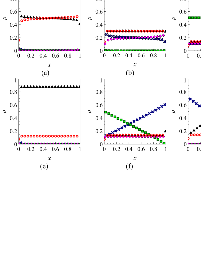
Figure 4. Time-average densities in 5-species odd mLPASEP for species $\overline{2}$ (red circles), $\overline{1}$ (magenta diamonds), 0 (green boxes), 1 (blue crosses) and 2 (black triangles) for (a) phase $\overline{\vvmathbb{2}}$ ($\lambda_{1}\simeq 0.36,\lambda_{2}\simeq 0.8,b\simeq 0.59$), (b) phase $\overline{\vvmathbb{1}}$ ($\lambda_{1}\simeq 0.37,\lambda_{2}\simeq 2.33,b\simeq 0.59$), (c) phase $\vvmathbb{0}$ ($\lambda_{1}\simeq 3.04,\lambda_{2}\simeq 6.16,b\simeq 2.61$), (d) phase $\vvmathbb{1}$ ($\lambda_{1}\simeq 3.04,\lambda_{2}\simeq 6.16,b\simeq 4.91$), (e) phase $\vvmathbb{2}$ ($\lambda_{1}\simeq 3.02,\lambda_{2}\simeq 6.09,b\simeq 7.15$), (f) $\vvmathbb{0}-\vvmathbb{1}$ coexistence line ($\lambda_{1}=3,\lambda_{2}\simeq 6.41,b=3$), and (g) $\vvmathbb{1}-\vvmathbb{2}$ coexistence line ($\lambda_{1}\simeq 3.05,\lambda_{2}=6,b=6$). The lattice size is $1000$ for all cases.

The simplest nontrivial odd mLPASEP is the one with five species. The boundary transitions are given by

Left:	$\begin{cases}\overline{2},\overline{1},0,1\rightarrow 2\quad\text{ with rate }\alpha_{2},\\ \overline{2},\overline{1},0\rightarrow 1\quad\text{ with rate }\alpha_{1},\\ \overline{2},\overline{1}\rightarrow 0\quad\text{ with rate }\alpha_{0},\\ 1,2\rightarrow 0\quad\text{ with rate }\gamma_{0},\\ 2\rightarrow 1\quad\text{ with rate }\gamma_{1},\end{cases}$
Right:	$\begin{cases}2\rightarrow\overline{2}\quad\text{ with rate }\beta,\\ 1\rightarrow\overline{1}\quad\text{ with rate }\beta,\\ \overline{1}\rightarrow 1\quad\text{ with rate }\delta,\\ \overline{2}\rightarrow 2\quad\text{ with rate }\delta.\par\end{cases}$

In the 1-colouring, we identify species 1’s and 2’s as $1_{1}$, $\overline{1}$’s and $\overline{2}$’s as $\overline{1}_{1}$, and 0’s as $0_{1}$, such that the rates for boundary transitions are given by

Left:	$\begin{cases}\overline{1}_{1},0_{1}\rightarrow 1_{1}\quad\text{ with rate }\theta_{1},\\ \overline{1}_{1}\rightarrow 0_{1}\quad\text{ with rate }\phi_{1},\\ 1_{1}\rightarrow 0_{1}\quad\text{ with rate }\zeta_{1},\end{cases}$
Right:	$\begin{cases}1_{1}\rightarrow\overline{1}_{1}\quad\text{ with rate }\beta,\\ \overline{1}_{1}\rightarrow 1_{1}\quad\text{ with rate }\delta.\end{cases}$

The relevant left and right boundary parameters are $\lambda_{1}$ and $b=\kappa_{\beta,\delta}^{+}$ respectively. On the other hand, we label $\overline{1}$’s,0’s and 1’s with $0_{2}$, $2$’s with $1_{2}$, and $\overline{2}$’s with $\overline{1}_{2}$ in 2-colouring. Now, we have the following boundary rates

Left:	$\begin{cases}\overline{1}_{2},0_{2}\rightarrow 1_{2}\quad\text{ with rate }\theta_{2},\\ \overline{1}_{2}\rightarrow 0_{2}\quad\text{ with rate }\phi_{2},\\ 1_{2}\rightarrow 0_{2}\quad\text{ with rate }\zeta_{2},\end{cases}$
Right:	$\begin{cases}1_{2}\rightarrow\overline{1}_{2}\quad\text{ with rate }\beta,\\ \overline{1}_{2}\rightarrow 1_{2}\quad\text{ with rate }\delta.\end{cases}$

The relevant parameters $\lambda_{2}$ and $b=\kappa_{\beta,\delta}^{+}$ correspond to the left and right boundary respectively.

Figure 5. Phase diagram for mLPASEP with $r=2$. The shaded region ($\lambda_{1}>\lambda_{2}$) is forbidden. The plane in focus is given by $\lambda_{2}=s_{1}\lambda_{1}$.

The phase diagram is the three-dimensional space of the parameters $\lambda_{1},\lambda_{2}$ and $b$. The region $\lambda_{1}>\lambda_{2}$ is excluded. We fix a constant $s_{1}>1$ and consider the two dimensional plane $\lambda_{2}=s_{1}\lambda_{1}$. In this plane, $\lambda$ is the distance along the $b=0$ plane. This plane passes through all the phases and, as a result, allows us to visualize all phases on a two-dimensional phase diagram as shown in Figure 5. Using the colouring ideas as outlined in Section 4, we find that there are five phases in the phase diagram:

• phase $\overline{\vvmathbb{2}}$: $\max\left\{b,\lambda_{2}\right\}<1$,

• phase $\overline{\vvmathbb{1}}$: $\max\left\{b,\lambda_{1}\right\}<1<\lambda_{2}$,

• phase $\vvmathbb{0}$: $\max\left\{1,b\right\}<\lambda_{1}$,

• phase $\vvmathbb{1}$: $\max\left\{1,\lambda_{1}\right\}<b<\lambda_{2}$,

• phase $\vvmathbb{2}$: $\max\left\{1,\lambda_{2}\right\}<b$.

In addition, the two co-existence planes, the $\vvmathbb{0}-\vvmathbb{1}$ phase boundary: $1<b=\lambda_{1}$ , and the $\vvmathbb{1}-\vvmathbb{2}$ phase boundary: $1<b=\lambda_{2}$, appear as lines. On the $b=0$ plane, the plane $\lambda_{i}=1$ and the plane $\lambda_{2}=s_{1}\lambda_{1}$ intersect at the point denoted by $A_{i}$ for $i=1,2$. $A_{1}$ and $A_{2}$ have locations $(1,s_{1},0)$ and $(1/s_{1},1,0)$.

5. The shock picture in the odd mLPASEP

We now use the shock picture in the LPASEP to understand the density profiles as well as the phenomenon of dynamical expulsion in the odd mLPASEP. We will explain this picture in each phase and phase-boundary. This picture is best understood by looking at the coexistence lines first.

Figure 6. The shock picture for mLPASEP: The schematic plot shows the shock on the co-existence line $b=\lambda_{j}>1$ for the odd mLPASEP where $1\leq j\leq r$. At each point $x$, the densities of the $k$-coloured species $1_{k}$ and $\overline{1}_{k}$ satisfy (8) for each $k$.

The $(\vvmathbb{j}-\vvmathbb{1})-\vvmathbb{j}$ coexistence line for $1\leq j\leq r$: From the $k$-colouring argument, we see that species $j-1$ and $j$ are phase-segregated and other species have constant densities on this coexistence line. In other words, only species $j-1$ and $j$ take part in the shock on this coexistence line. This is illustrated in the schematic plot in Figure 6. The shock performs a random walk with no net drift. Moreover, species $\overline{j-1},\ldots,j-2$ are dynamically expelled. See Figure 4(f) and (g) for simulations of the odd mLPASEP with $r=2$ on the $\vvmathbb{0}-\vvmathbb{1}$ and $\vvmathbb{1}-\vvmathbb{2}$ coexistence lines respectively. See also Figures 7 (a) and (b) for instantaneous profiles of the shock in these lines.

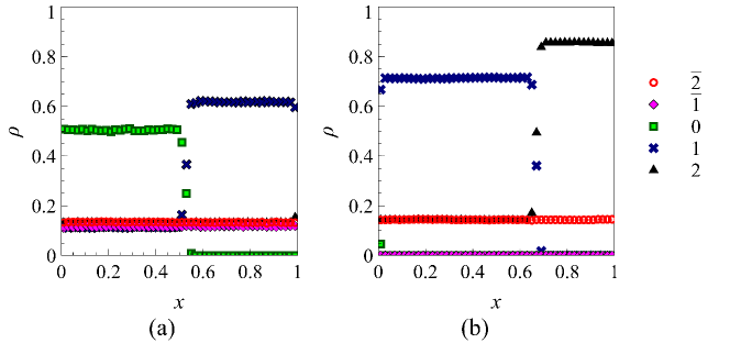
Figure 7. Instantaneous shock profiles in 5-species odd mLPASEP : Density profiles for species $\overline{2}$ (red circles), $\overline{1}$ (magenta diamonds), 0 (green boxes), 1 (blue crosses) and 2 (black triangles) on (a) $\vvmathbb{0}-\vvmathbb{1}$ coexistence line ($\lambda_{1}=3,\lambda_{2}\simeq 6.41,b=3$), and (b) $\vvmathbb{1}-\vvmathbb{2}$ coexistence line ($\lambda_{1}\simeq 3.05,\lambda_{2}=6,b=6$), where the lattice size is $2500$.

Phases $\overline{\vvmathbb{j}}$ and $\vvmathbb{j}$ for $1\leq j\leq r$: In phase $\vvmathbb{j}$, the shock front is pinned to the left causing the dynamical expulsion of species $j-1$ and higher density of $j$’s compared to $\overline{j}$’s. In phase $\overline{\vvmathbb{j}}$, the $j-1$’s are again dynamically expelled because the height of the shock vanishes. See Figure 4(a), (b), (d) and (e) for simulations of the odd mLPASEP with $r=2$ in phases $\overline{\vvmathbb{2}},\overline{\vvmathbb{1}},\vvmathbb{1}$ and $\vvmathbb{2}$.

Phase $\vvmathbb{0}$: The shock picture on the $\vvmathbb{0}-\vvmathbb{1}$ coexistence line is Figure 6 with $j=1$. The shock front has positive drift in phase $\vvmathbb{0}$ and consequently gets pinned to the right boundary resulting in non-zero bulk density of species 0. Hence, all species have non-zero densities in phase $\vvmathbb{0}$. See Figure 4(c) for simulations of the odd mLPASEPwith $r=2$ in phase $\vvmathbb{0}$.

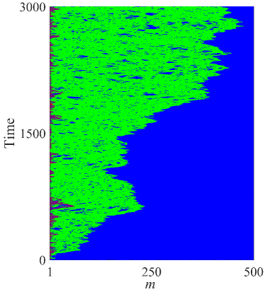
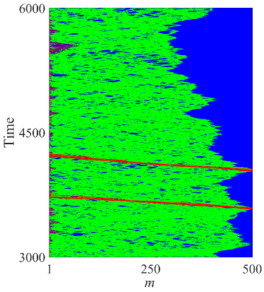
(a)	(b)

Figure 8. The spatio-temporal evolution of the shock on the $\vvmathbb{1}-\vvmathbb{2}$ co-existence line for 5-species odd mLPASEP for 6000 time steps. Each time step equals 4000 random sequential updates in the simulation. The plots show trajectories of species $\overline{1}$ (red), 0 (violet), 1 (green) and 2 (blue) versus site position after the system reaches steady state. Particles of species $\overline{2}$ are not shown. The parameters are as follows: $\alpha_{\overline{1}}=0.08,\alpha_{0}=0.45,\alpha_{1}=0.13,\alpha_{2}=0.33,\gamma_{0}\simeq 0.005,\gamma_{1}\simeq 0.06,q=0.1,\beta=0.475,\ \text{and}\ \delta=0.35\,(b=\lambda_{2}=2,\lambda_{1}\simeq 0.98)$, and the lattice size is $500$.

In addition, we note the following on the $(\vvmathbb{j}-\vvmathbb{1})-\vvmathbb{j}$ coexistence line. Species $\overline{j-1}$ is dynamically expelled on this line, although species $j-1$ has non-zero bulk density. This might seem counterintuitive because (8) suggests that either a species and its barred partner are both present or both absent. The resolution of this apparent contradiction is the fact that (8) only applies to the $k$-coloured species $\overline{1}_{k}$ and $1_{k}$ for each $k$.

To illustrate this point further, we perform a spatio-temporal simulation of the odd mLPASEP with $r=2$ on the $\vvmathbb{1}-\vvmathbb{2}$ coexistence line. The results of the simulation are shown in Figure 8. The shock there is formed between species 1 and 2 and has zero mean velocity. Species $0$ and $\overline{1}$ are dynamically expelled. As one can see from the simulation, particles of species $\overline{1}$ can enter either on the left or the right boundary, but they eventually leave from the left boundary because of the high density of 1’s and 2’s. They can only enter at the right boundary when the $1-2$ shock touches the right boundary.

6. Conclusion

In this article, we have defined a multispecies ASEP and determined the exact phase diagram corresponding to the model. The structure of the phase diagram derived by the colouring method is the same when there are either $2r$ or $(2r+1)$-species in the model. It would be an interesting problem to find a matrix ansatz for the mLPASEP so that the densities and currents can be computed directly. The phase diagram of LPASEP has a rich structure that manifests itself in the presence of subphases inside the LD and HD phases. One might turn to the colouring technique to unearth the subphases in the phase diagram for the mLPASEP.

Appendix A The even mLPASEP

We explain the salient features of the phase diagram of the even mLPASEP focusing on the aspects that make the analysis more complicated than that for the odd mLPASEP.

The computation of the generalized phase diagram for the even mLPASEP requires us to project to the single-species ASEP [22] which we review briefly. The ASEP involves only particles and vacancies, denoted by 1 and $\overline{1}$ respectively. The boundary transitions, in accord with our definitions in Eq. (5) and (4), have the following rates:

Left:	$\begin{cases}\overline{1}\rightarrow 1\quad\text{ with rate }\alpha_{1},\\ 1\rightarrow\overline{1}\quad\text{ with rate }\gamma^{\prime}_{0},\end{cases}$
Right:	$\begin{cases}1\rightarrow\overline{1}\quad\text{ with rate }\beta,\\ \overline{1}\rightarrow 1\quad\text{ with rate }\delta.\end{cases}$

The relevant left and right boundary parameters are $\lambda=\kappa_{\alpha_{1},\gamma^{\prime}_{0}}^{+}$ and $b=\kappa_{\beta,\delta}^{+}$ respectively, where $\kappa^{\pm}_{u,v}$ is defined in (7). With this notation, the phase diagram formally looks exactly like Figure 1 with the same nomenclature for the phases: phase $\overline{\vvmathbb{1}}$ (MC), $\vvmathbb{0}$ (LD) and $\vvmathbb{1}$ (HD). The currents and densities of species $1$ for all three phases are also identical to those in Table 1. The density profiles for ASEP can also be understood by appealing to shocks. Since this is reviewed by Blythe and Evans in [2], we only illustrate the shock picture for the coexistence line $b=\lambda>1$ in Figure 9, where the shock has zero mean velocity. In the LD (resp. HD) phase, the shock has positive (resp. negative) velocity and is pinned to the right (resp. left).

Figure 9. The shock picture for ASEP on the co-existence line $b=\lambda>1$.

The phase diagrams for the even mLPASEP with $2r$ species and the odd mLPASEP with $(2r+1)$ species have identical structure as depicted in Figure 3. The main difference between the two is that the $1$-colouring projects the even mLPASEP to the ASEP so that the boundary parameters are $\lambda_{1}=\kappa^{+}_{\theta_{1},\gamma^{\prime}_{0}}$ and $b=\kappa^{+}_{\beta,\delta}$. All other $k$-colourings continue to project the even mLPASEP to the LPASEP with boundary parameters $\lambda_{k}=\theta_{k}/\phi^{\prime}_{k}$ and $b=\kappa^{+}_{\beta,\delta}$., where $\theta_{k}=\sum_{i=k}^{r}\alpha_{i}$ and $\phi^{\prime}_{i}=\sum_{i=1}^{k-1}\left(\alpha_{i}+\alpha_{\overline{i}}\right)$ were defined in Section 2.2.

Taking into account all possible colourings, there are $r+1$ relevant boundary parameters, namely, $\lambda_{1},\ldots,\lambda_{r}$ and $b$. Again, the inequalities $\lambda_{1}<\lambda_{2}<\ldots<\lambda_{r}$ are satisfied. Because of these relations among $\lambda_{i}$’s, we arrive at the same phase diagram in Figure 3 which shows all $2r+1$ phases in the even mLPASEP. In all phases except phase $\vvmathbb{0}$, the densities of all species have the same expression in the even mLPASEP as given in Table 2. In phase $\vvmathbb{0}$, the densities of $1$ and $\overline{1}$ are $(f(\lambda_{1})-f(\lambda_{2}))$ and $(\overline{f}(\lambda_{1})-f(\lambda_{2}))$ respectively. We illustrate the density profiles with simulations for the $4$-species even mLPASEP in Figure 10.

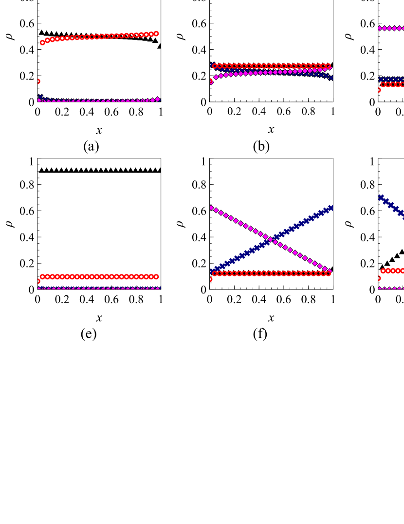
Figure 10. Time-average densities in 4-species mLPASEP for species $\overline{2}$ (red circles), $\overline{1}$ (magenta diamonds), 0 (green boxes), 1 (blue crosses) and 2 (black triangles) for (a) phase $\overline{\vvmathbb{2}}$ ($\lambda_{1}\simeq 0.23,\lambda_{2}\simeq 0.84,b\simeq 0.65$), (b) phase $\overline{\vvmathbb{1}}$ ($\lambda_{1}\simeq 0.44,\lambda_{2}\simeq 2.65,b\simeq 0.75$), (c) phase $0$ ($\lambda_{1}\simeq 2.27,\lambda_{2}\simeq 6.5,b\simeq 0.92$), (d) phase $\vvmathbb{1}$ ($\lambda_{1}\simeq 1.17,\lambda_{2}\simeq 6.45,b\simeq 3.09$), (e) phase $\vvmathbb{2}$ ($\gamma_{1}\simeq 0.12,q=0.41,\beta=0.15,\delta=0.86,\lambda_{1}\simeq 1.17,\lambda_{2}\simeq 6.45,b\simeq 9.28$), (f) $\vvmathbb{0}-\vvmathbb{1}$ co-existence line ($\lambda_{1}=3,\lambda_{2}\simeq 7.18,b=3$), and (g) $\vvmathbb{1}-\vvmathbb{2}$ co-existence line ($\lambda_{1}\simeq 1.34,\lambda_{2}=6,b=6$). For all simulations, we fix the lattice size to be $1000$.

The shock picture in the even mLPASEP is identical to that in the odd mLPASEP in all coexistence lines except the $\vvmathbb{0}-\vvmathbb{1}$ boundary.

On this coexistence line, $1$’s and $\overline{1}$’s form a shock with zero drift as shown in Figure 11. The shock is pinned to the right (resp. left) boundary in phase $\vvmathbb{0}$ (resp. $\vvmathbb{1}$). In phase $\overline{\vvmathbb{1}}$, the density of these two species become equal and the height of the shock goes to zero as the system approaches this phase along the $\vvmathbb{0}-\vvmathbb{1}$ coexistence line. We have performed simulations showing instantaneous density profiles for the even mLPASEP with 4 species on the $\vvmathbb{0}-\vvmathbb{1}$ boundary and the results exactly match with the theoretical prediction.

Figure 11. The shock picture for the even mLPASEP on the $\vvmathbb{0}-\vvmathbb{1}$ co-existence line.

References

- [1] B Derrida, M R Evans, V Hakim, and V Pasquier. Exact solution of a 1d asymmetric exclusion model using a matrix formulation. Journal of Physics A: Mathematical and General, 26(7):1493, 1993.
- [2] R A Blythe and M R Evans. Nonequilibrium steady states of matrix-product form: a solver’s guide. Journal of Physics A: Mathematical and Theoretical, 40(46):R333, 2007.
- [3] Andreas Schadschneider. Traffic flow: a statistical physics point of view. Physica A: Statistical Mechanics and its Applications, 313(1):153 – 187, 2002. Fundamental Problems in Statistical Physics.
- [4] Debashish Chowdhury, Ludger Santen, and Andreas Schadschneider. Statistical physics of vehicular traffic and some related systems. Physics Reports, 329(4):199 – 329, 2000.
- [5] Catherine J. Penington, Barry D. Hughes, and Kerry A. Landman. Building macroscale models from microscale probabilistic models: A general probabilistic approach for nonlinear diffusion and multispecies phenomena. Phys. Rev. E, 84:041120, Oct 2011.
- [6] M. R. Evans, D. P. Foster, C. Godrèche, and D. Mukamel. Asymmetric exclusion model with two species: Spontaneous symmetry breaking. Journal of Statistical Physics, 80(1):69–102, Jul 1995.
- [7] Chikashi Arita. Phase transitions in the two-species totally asymmetric exclusion process with open boundaries. Journal of Statistical Mechanics: Theory and Experiment, 2006(12):P12008, 2006.
- [8] Masaru Uchiyama. Two-species asymmetric simple exclusion process with open boundaries. Chaos, Solitons and Fractals, 35(2):398 – 407, 2008.
- [9] Arvind Ayyer, Joel L. Lebowitz, and Eugene R. Speer. On the two species asymmetric exclusion process with semi-permeable boundaries. Journal of Statistical Physics, 135(5):1009–1037, Jun 2009.
- [10] Arvind Ayyer, Joel L. Lebowitz, and Eugene R. Speer. On some classes of open two-species exclusion processes. Markov Processes And Related Fields, 18(5):157–176, 2012.
- [11] N Crampe, K Mallick, E Ragoucy, and M Vanicat. Open two-species exclusion processes with integrable boundaries. Journal of Physics A: Mathematical and Theoretical, 48(17):175002, 2015.
- [12] N Crampe, M R Evans, K Mallick, E Ragoucy, and M Vanicat. Matrix product solution to a 2-species TASEP with open integrable boundaries. Journal of Physics A: Mathematical and Theoretical, 49(47):475001, 2016.
- [13] Arvind Ayyer, Caley Finn, and Dipankar Roy. Matrix product solution of a left-permeable two-species asymmetric exclusion process. Phys. Rev. E, 97:012151, Jan 2018.
- [14] Martin R. Evans, Pablo A. Ferrari, and Kirone Mallick. Matrix representation of the stationary measure for the multispecies TASEP. Journal of Statistical Physics, 135(2):217–239, Apr 2009.
- [15] S Prolhac, M R Evans, and K Mallick. The matrix product solution of the multispecies partially asymmetric exclusion process. Journal of Physics A: Mathematical and Theoretical, 42(16):165004, 2009.
- [16] Pablo A. Ferrari and J. B. Martin. Multi-class processes, dual points and M/M/1 queues. Markov Process. Related Fields, 12(2):175–201, 2006.
- [17] Pablo A. Ferrari and James B. Martin. Stationary distributions of multi-type totally asymmetric exclusion processes. The Annals of Probability, 35(3):807–832, 05 2007.
- [18] Arvind Ayyer and Svante Linusson. Correlations in the multispecies TASEP and a conjecture by lam. Trans. Amer. Math. Soc., 369(2):1097–1125, 2017.
- [19] Luigi Cantini, Alexandr Garbali, Jan de Gier, and Michael Wheeler. Koornwinder polynomials and the stationary multi-species asymmetric exclusion process with open boundaries. Journal of Physics A: Mathematical and Theoretical, 49(44):444002, 2016.
- [20] Arvind Ayyer and Dipankar Roy. The exact phase diagram for a class of open multispecies asymmetric exclusion processes. Scientific Reports, 7:13555–, Oct 2017.
- [21] N Crampe, C Finn, E Ragoucy, and M Vanicat. Integrable boundary conditions for multi-species ASEP. Journal of Physics A: Mathematical and Theoretical, 49(37):375201, 2016.
- [22] Masaru Uchiyama, Tomohiro Sasamoto, and Miki Wadati. Asymmetric simple exclusion process with open boundaries and Askey–Wilson polynomials. Journal of Physics A: Mathematical and General, 37(18):4985, 2004.