Lifted Wasserstein Matcher for Fast and Robust Topology Tracking

Abstract

This paper presents a robust and efficient method for tracking topological features in time-varying scalar data. Structures are tracked based on the optimal matching between persistence diagrams with respect to the Wasserstein metric. This fundamentally relies on solving the assignment problem, a special case of optimal transport, for all consecutive timesteps. Our approach relies on two main contributions. First, we revisit the seminal assignment algorithm by Kuhn and Munkres which we specifically adapt to the problem of matching persistence diagrams in an efficient way. Second, we propose an extension of the Wasserstein metric that significantly improves the geometrical stability of the matching of domain-embedded persistence pairs. We show that this geometrical lifting has the additional positive side-effect of improving the assignment matrix sparsity and therefore computing time. The global framework computes persistence diagrams and finds optimal matchings in parallel for every consecutive timestep. Critical trajectories are constructed by associating successively matched persistence pairs over time. Merging and splitting events are detected with a geometrical threshold in a post-processing stage. Extensive experiments on real-life datasets show that our matching approach is up to two orders of magnitude faster than the seminal Munkres algorithm. Moreover, compared to a modern approximation method, our approach provides competitive runtimes while guaranteeing exact results. We demonstrate the utility of our global framework by extracting critical point trajectories from various time-varying datasets and compare it to the existing methods based on associated overlaps of volumes. Robustness to noise and temporal resolution downsampling is empirically demonstrated.

Introduction

Performing feature extraction and object tracking is an important topic in scientific visualization, for it is key to understanding time-varying data. Specifically, it allows to detect and track the evolution of regions of interest over time, which is central to many scientific domains, such as combustion [8], aerodynamics [35], oceanography [62] or meteorology [94]. With the increasing power of computational resources and resolution of acquiring devices, efficient methods are needed to enable the analysis of large datasets.

The emergence of new paradigms for scientific simulation, such as in-situ and in-transit [2, 93, 63, 57, 49], clearly exhibits the ambition to reach toward exascale computing [17] in the forthcoming years. In this context, as both spatial and temporal resolutions of acquired or simulated datasets keep on increasing, understanding the evolution of features of interest throughout time proves challenging.

Topological data analysis has been used in the last decades as a robust and reliable setting for hierarchically defining features in scalar data [22]. In particular, its successful application to time-varying data [75, 9] makes it a prime candidate for tracking. Both topological analysis and feature tracking have been applied in-situ [95, 44], which demonstrates their interest in the context of large-scale data. Nonetheless, major bottlenecks of state-of-the art topology tracking methods are still the high required computation cost as well as the need for high temporal resolution.

In this paper, we propose a novel feature-tracking framework, which correlates topological features in time-varying data in an efficient and meaningful way. It is the first approach, to the best of our knowledge, combining the setting of topological data analysis with optimal transport for the problem of feature tracking. More precisely, the key idea is to use combinatorial optimization for matching topological structures (namely, persistence diagrams) according to a fine-tuned metric. After exposing our formal setting (Sec. 1), we introduce an extension of the exact assignment algorithm by Kuhn and Munkres [43, 51] that we adapt in an efficient way to the case of persistence diagrams (Sec. 2). We highlight the issues raised by the classical Wasserstein metric between diagrams, and propose a robust lifted metric that overcomes these limitations (Sec. 3). We then present the detailed tracking framework (Sec. 4). Extensive experiments demonstrate the utility of our approach (Sec. 5).

0.1 Related work

Our framework encompasses the definition, correlation and tracking of topological features in scalar fields. As such, it is related to topological data analysis of scalar fields, tracking techniques, the definition of metrics and combinatorial optimization.

Topological analysis techniques [22, 54, 36, 20] have demonstrated their ability over recent years to capture features of interest in scalar data in a generic, robust [24, 15] and efficient manner, for many applications as turbulent combustion [8], computational fluid dynamics [25], material sciences [34], chemistry [29], astrophysics [78], medical imaging [12, 6]. One reason for their success in applications is the possibility for domain experts to easily translate high level structural notions into topological abstractions, such as contour trees [11], Reeb Graphs [53, 5], Morse-Smale complexes [32]. For instance, in astrophysics the cosmic web can be extracted by querying the most persistent 1-separatrices of the Morse-Smale complex connected to maxima of matter density [78]. Similar domain-specific notions are translated into topological terms in the above examples.

Feature tracking: Topology has been used for feature extraction and tracking in the context of vector fields [87, 56, 61], mostly relying on stream lines, path lines [79, 80, 81, 69, 68], or tracking punctual singularities [42]. For the latter, a forward streamline integration of critical points is performed in a specific scale space, which adapted for time-varying data would require knowledge about the evolution of the field, and for instance to compute time-derivatives.

For scalar data, features are defined based on attributes that are either geometric (isosurfaces, thresholded regions), or topological (contour trees, Reeb graphs). Similarly, tracking approaches either rely on geometrical (volume overlaps, distance between centers of gravity) or topological extracts (Jacobi set, segment overlap).

Geometrical approaches are based on thresholded connected components [74], glyphs [59], cluster tracking [27], petri nets [52], or propose a hierarchical representation [28]. Similarly, the core methodology for associating topological features for tracking is often based on overlaps of geometrical domains along with other attributes [66, 9, 8, 75, 70, 71, 72, 73], on tracking Jacobi sets [21, 23], or matching isosurfaces in higher-dimensional spaces [37, 39].

Such approaches usually test features in two consecutive timesteps against one another for potential overlaps, then draw the best correspondence between features according to some criterion. Typical criteria include optimizing the overlapping volume, mass, distance between centroids, or a combination of these [67, 59]. For this to work, the temporal sampling rate of the underlying data must be such that features in two consecutive timesteps effectively overlap. This first criterion is thus not very robust to temporal downsampling.

Other approaches rely on global optimization [38], using the Earth Mover’s distance [46] between geometrical features with various attributes such as centroid position, volume and mass. This does not, however, benefit from the natural definition of features offered by topological data analysis, nor from the possibility to simplify features in a hierarchical way. This is a real drawback in the context of noisy data as it implies dealing with large, computation-intensive optimization problems between every pair of timesteps.

Once features have been defined, and a methodology established to associate them in consecutive timesteps, the tracking representation is quite independent of whether geometrical or topological arguments have been used. Most often, graphs are used [64, 92, 45], such as Reeb graphs [91, 23] and nested tracking graphs [47]. Many popular graph structures are accounted for in [89]. An inconvenience of extracting rich tracking structures such as these without taking careful attention to potential noise is that it makes the interpretation quite difficult. In [8], the tracking graph is dense and intricate, making exploration impractical. It is therefore mandatory to do filtering and simplification in a post-processing stage, or to cleverly discard noisy events beforehand.

Assignment problems: Since we revisit the original algorithm by Kuhn and Munkres, we discuss here some related work in combinatorial optimization. The assignment problem is the discrete optimization problem consisting of finding a perfect matching of optimal cost in a weighted bipartite graph [51, 3, 10]. In other terms, the problem is to find an optimal one-to-one correspondence between discrete entities (such as singularities in a scalar field at two different timesteps), with a cost associated to each possible correspondence. It can be solved with the seminal Kuhn-Munkres algorithm [51]. The auction algorithm [3, 4, 41] is another popular approach for solving the assignment problem with a user-defined error threshold on the resulting assignment cost. In practice, this threshold is often set to 1% of the scalar range. A more general, continuous formulation of this problem is at the heart of Transportation theory [48, 40, 88]. Modern techniques [19] have attracted acute interest for making this theoretical setup central to shape correlation [77] and interpolation [76], which do bear resemblance to feature tracking.

Metrics: Since we introduce a new metric for the matching of persistence diagrams, we discuss in the following existing metrics traditionally used in topological data analysis. The Bottleneck and the interleaving distances [15, 14] have been widely investigated to study the stability of persistence diagrams. These metrics have been notably adapted in the context of kernel methods [60, 13] in machine learning. In particular, the Bottleneck distance is a special case of the more general Wasserstein metric [48, 40] applied to diagram points, also known as the Earth Mover’s Distance [46]. The standard approach for computing the discrete Wasserstein metric relies on solving the associated assignment problem, either with an exact Kuhn-Munkres approach [50, 90] or with an auction-based approximation [41]. However, as discussed in Sec. 3, when these methods (metric-based [14, 15] or kernel-based [60, 13]) are applied as-is for tracking purposes, a high geometrical instability occurs which impairs the tracking robustness, as already observed in the case of vineyards [16]. Our work (see Sec. 3) addresses this issue.

0.2 Contributions

This paper makes the following new contributions:

1. Approach: We present a sound and original framework, which is the first combining topology and transportation for feature tracking, comparing favorably to other state-of-the-art approaches, both in terms of speed and robustness.

2. Metric: We extend traditional topological metrics, for the needs of time-varying feature tracking, notably enhancing geometrical stability and computing time.

3. Algorithm: We extend the assignment method by Kuhn and Munkres to solve the problem of persistence matchings in a fast and exact way, taking advantage of our metric.

1 Preliminaries

This section describes our formal setting and presents an overview of our approach. It contains definitions that we adapted from Tierny et al. [84]. An introduction to topology can be found in [22].

1.1 Background

Input data: Without loss of generality, we assume that the input data is a piecewise linear (PL) scalar field $f:\mathcal{M}\rightarrow\mathbb{R}$ defined on a PL $d$-manifold $\mathcal{M}$ with $d\leq 3$. Values are given at the vertices of $\mathcal{M}$ and linearly interpolated on higher dimension simplices.

Critical points: Given an isovalue $i\in\mathbb{R}$, the sub-level set of $i$, noted $f^{-1}_{-\infty}(i)$, is the pre-image of the open interval $(-\infty,i)$ onto $\mathcal{M}$ through $f$: $f^{-1}_{-\infty}(i)=\{p\in\mathcal{M}\leavevmode\nobreak\ |\leavevmode\nobreak\ f(p)<i\}$. The sur-level set is symmetrically given by $f^{-1}_{+\infty}(i)=\{p\in\mathcal{M}\leavevmode\nobreak\ |\leavevmode\nobreak\ f(p)>i\}$. These two objects serve as segmentation tools in many analysis tasks [8].

The points $p\in\mathcal{M}$ where the topology of $f^{-1}_{-\infty}(f(p)-\epsilon)$ differs from that of $f^{-1}_{-\infty}(f(p)+\epsilon)$ are the critical points of $f$ and their values are called critical values. Critical points can be classified with their index $\mathcal{I}$, which is 0 for minima, 1 for 1-saddles, $d-1$ for $(d-1)$-saddles and $d$ for maxima, with $d$ the dimension of $\mathcal{M}$.

Persistence diagrams: The distribution of critical points of $f$ can visually be represented by a topological abstraction called the persistence diagram [24, 15] (Fig. 1). By applying the Elder Rule [22], critical points can be arranged in a set of pairs, such that each critical point appears in only one pair $(c_{i},c_{j})$ with $f(c_{i})<f(c_{j})$ and $\mathcal{I}(c_{i})=\mathcal{I}(c_{j})-1$. More precisely, the Elder Rule states that as the value $i$ increases, if two topological features of $f^{-1}_{-\infty}(i)$, for instance two connected components, meet at a given saddle $c_{j}$ of $f$, the youngest of the two (the one with the highest minimal value, $c_{i}$) dies at the advantage of the oldest (the one with the lowest minimal value). Critical points $c_{i}$ and $c_{j}$ then form a persistence pair.

The persistence diagram $\mathcal{D}(f)$ embeds each pair $(c_{i},c_{j})$ in the plane such that its horizontal coordinate equals $f(c_{i})$, and the vertical coordinate of both $c_{i}$ and $c_{j}$ is $f(c_{i})$ and $f(c_{j})$, corresponding respectively to the birth and death of the pair. The height of the pair $P(c_{i},c_{j})=|f(c_{j})-f(c_{i})|$ is called the persistence and denotes the life-span of the topological feature created at $c_{i}$ and destroyed at $c_{j}$. In three dimensions, the persistence of the pairs linking critical points of index $(0,1)$, $(2,3)$ and $(1,2)$ denotes the life-span of connected components, voids and non-collapsible cycles of $f^{-1}_{-\infty}(i)$.

Figure 1: Four gaussians defined on a 2D plane (top left) and the associated persistence diagram (right); three gaussians defined on a 3D volume (bottom left) with persistence diagram (right). The most prominent topological features are those which have the longest lifespan, and correspond to the longest vertical bars in persistence diagrams.

In practice, persistence diagrams serve as an important visual representation of the distribution of critical points in a scalar data-set. Small oscillations in the data due to noise are typically represented by critical point pairs with low persistence, in the vicinity of the diagonal. In contrast, topological features that are the most prominent in the data are associated with large vertical bars (Fig. 1). In many applications, persistence diagrams help users as a visual guide to interactively tune simplification thresholds in multi-scale data segmentation tasks based on the Reeb graph [58, 12, 53, 85, 30, 83] or the Morse-Smale complex [32, 33, 65].

Wasserstein distance: Metrics have been defined to evaluate the distance between two scalar fields $f,g:\mathcal{M}\rightarrow\mathbb{R}$. The $L$-norm $||f-g||_{\nu}$, is a classical example. In the context of topological data analysis, multiple metrics [15, 14] have been introduced in order to compare persistence diagrams. In our context, such metrics are key to identifying zones in the data which are similar to one another. Persistence diagrams can be associated with a pointwise distance, noted $d_{\nu}$ inspired by the $L$-norm. Given persistence pairs $a=(a_{x},a_{y})\in\mathcal{D}(f)$ and $b=(b_{x},b_{y})\in\mathcal{D}(g)$, $d_{\nu}$ is given by Eq. 1:

$$\begin{split}d_{\nu}(a,b)&=(|a_{x}-b_{x}|^{\nu}+|a_{y}-b_{y}|^{\nu})^{1/\nu}\\ \end{split}$$ (1)

The Wasserstein distance [48, 40], sometimes called the Earth Mover’s Distance [46], noted $d^{W}_{\nu}$, between the persistence diagrams $\mathcal{D}(f)$ and $\mathcal{D}(g)$ is defined in Eq. 2:

$$d^{W}_{\nu}\big{(}\mathcal{D}(f),\mathcal{D}(g)\big{)}=\min_{\phi\in\Phi}\bigg{(}\sum_{a\in\mathcal{D}(f)}d_{\nu}\big{(}a,\phi(a)\big{)}^{\nu}\bigg{)}^{1/\nu}$$ (2)

where $\Phi$ is the set of all possible bijections $\phi$ mapping each critical point $a$ of $\mathcal{D}(f)$ to a critical point $b$ of the same index $\mathcal{I}$ in $\mathcal{D}(g)$ or to the diagonal, noted $\text{diag}(a)$ – which corresponds to the removal of the corresponding feature from the assignment, with a cost $d(a,\text{diag}(a))$.

1.2 Assignment problem

The assignment problem is the problem of choosing an optimal assignment of $n$ workers $w\in W$ to $n$ jobs $j\in J$, assuming numerical ratings are given for each worker’s performance on each job.

Given ratings $r(w_{x},j_{y})$ are summed up in a cost matrix $(r_{xy})$, finding an optimal assignment means choosing a set of $n$ independent entries of the matrix so that the sum of these elements is optimal. Independent means than no two such elements should belong to the same row or column (i.e. no two workers should be assigned to the same job and no worker should be given more than one job). In other words, one must find a map $\sigma:W\rightarrow J$ of workers and jobs for which the sum $\sum_{x}(r(w_{x},\sigma(w_{x})))$ is optimal. There are $n!$ possible assignments, of which several may be optimal, so that an exhaustive search is impractical as $n$ gets large.

Similarly, the unbalanced assignment problem is the problem of finding an optimal assignment of $n$ workers to $m$ jobs, where some jobs or workers might be left unassigned. This is the case of assignments between sets of persistence pairs; where costs are defined for leaving specific pairs unassigned.

The Hungarian algorithm [43, 51] is the first polynomial algorithm proposed by Kuhn to solve the assignment problem. It is an iterative algorithm based on the following two properties:

Theorem 1

If a number is added or subtracted from all the entries of any one row or column of a cost matrix, then an optimal assignment for the resulting cost matrix is also an optimal assignment for the original cost matrix.

This means that the cost matrix $(r_{ij})$ can be replaced with $(r_{ij})-u_{i}-v_{j}$ where $u_{i}$ (resp. $v_{j}$) is an arbitrary number which is fixed for the $i^{th}$ row (resp. the $j^{th}$ column).

Theorem 2

If $R$ is a matrix and $m$ is the maximum number of independent zeros of $R$ (i.e. number of entries valued at 0), then there are $m$ lines (row or columns) which contain all the zeros of $R$.

This allows to determine whether an optimal assignment has been found and thus constitutes the stop criterion.

The algorithm iteratively performs additions and subtractions on lines and columns of the cost matrix, in a way that globally decreases the matrix cost, until the optimal assignment has been found, that is, until the matrix contains a set of $min(m,n)$ independent zeros.

In the remainder we consider the $O(min(m,n)^{2}max(m,n))$ unbalanced Kuhn-Munkres algorithm [51, 7], an improvement over Kuhn’s original version which follows the same principles, with an enhanced strategy for finding independent elements. The goal is always to reduce the cost matrix and find a maximal set of independent zeros. These independent zeros are marked with a star: they are candidates for the optimal assignment. Zeros which are candidates for being swapped with a starred zero are marked with a prime. Throughout the algorithm, rows and columns of the matrix are marked as covered to restrict the search for candidate zeros.

The algorithm can be seen as two alternating phases: a matrix reduction phase (Fig. 2) which makes new zeros appear, and an augmenting path phase (Fig. 3) which augments the number of marked (starred) independent zeros.

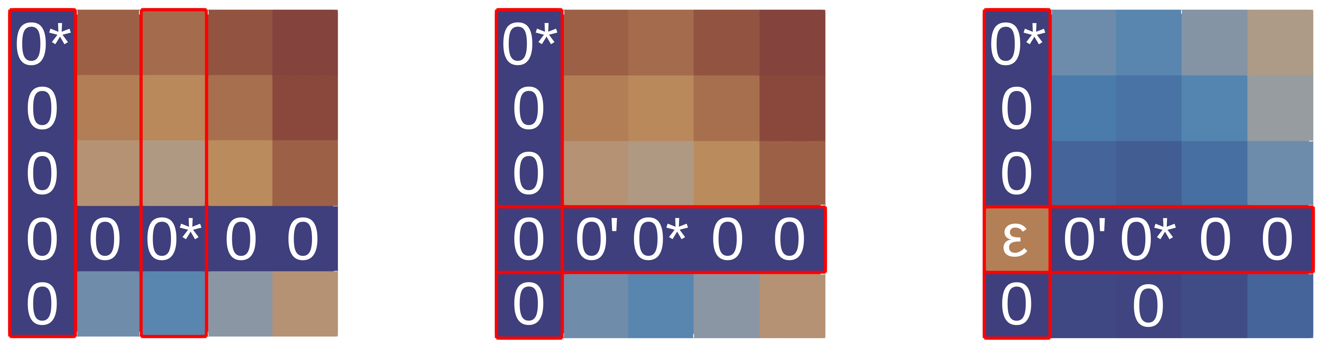
Figure 2: Matrix reduction phase. Subtracting the minimum element from each of the $n$ rows and columns might not be sufficient to make a set of $n$ independent zeros appear. In the above example, initially detected independent zeros are first starred. All columns containing a 0* are then covered (left). An uncovered zero which has a 0* in its row is found and primed; its row is covered and the column of the 0* is uncovered (center). At this point, all zeros are covered by construction. Let $\epsilon$ be the smallest uncovered value. Add $\epsilon$ to every covered row; subtract $\epsilon$ from every uncovered column. This amounts to decreasing uncovered elements by $\epsilon$ and increasing twice-covered elements by $\epsilon$. The sum of the elements of the matrix has been decreased and a new zero has appeared in an uncovered zone.

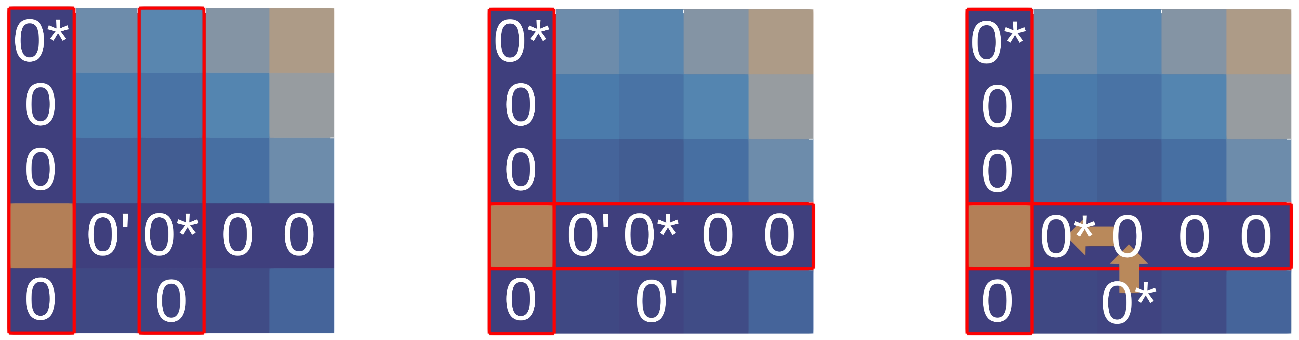
Figure 3: Augmenting path phase. After the first non-covered zero (left) is primed and covers updated, there is one non-covered zero $Z_{1}$ in the matrix (center), which is then primed. Let $Z_{2}$ be the 0* in the column of $Z_{1}$ (if any), let $Z_{3}$ be the 0’ in the row of $Z_{2}$ (there is one). Consider the series consisting of 0* ($Z_{2i}$) and 0’ ($Z_{2i+1}$) until it ends at a 0’ that has no 0* in its column. Unstar each 0*, star each 0’ of the series. The number of starred zeros has increased by one.

1.3 Persistence assignment problem

The assignment problem for persistence pairs is very similar to the standard unbalanced assignment problem, except additional costs are defined for not assigning elements (i.e. matching persistence pairs with the diagonal). The assignment between diagrams $P$ and $Q$ then involves $r_{ij}$ the numerical rating associated with assigning $p_{i}\in P$ with $q_{j}\in Q$, along with $r_{i,-1}$ (resp. $r_{-1,j}$) the numerical rating associated with matching $p_{i}$ (resp. $q_{j}$) with the diagonal.

If $P$ and $Q$ are sets of persistence pairs such that $card(P)=n$ and $card(Q)=m$, then it is possible to solve the persistence assignment problem using the standard Kuhn-Munkres algorithm with the $(n+m)\times(n+m)$ cost matrix described by Eq. 3, as proposed in [50]:

$$r_{ij}=\begin{cases}d_{\nu}(p_{i},q_{j})&{\scriptstyle\text{if $0<i\leq n,0<j\leq m$}}\\ d_{\nu}(q_{j},\text{diag}(q_{j}))&{\scriptstyle\text{if $n<i\leq m+n,0<j\leq m$}}\\ d_{\nu}(p_{i},\text{diag}(p_{i}))&{\scriptstyle\text{if $0<i\leq n,m<j\leq m+n$}}\\ 0&{\scriptstyle\text{if $n<i\leq m+n,m<j\leq n+m$}}\end{cases}$$ (3)

The first line corresponds to matching pairs from $P$ to pairs from $Q$; the second one corresponds to the possibility of matching pairs from $P$ to the diagonal; the third one is for matching pairs of $Q$ to the diagonal and the last one completes the cost matrix. The drawback of this approach is that it requires to solve the assignment problem on a $(n+m)^{2}$ cost matrix (that potentially contains two non-sparse blocks where persistence elements are located, see Fig. 4), though the number of distinct elements is at most $(n+1)\times(m+1)$. As seen in Sec. 2, our algorithm addresses this issue.

1.4 Overview

This section presents a quick overview of our tracking method, which is illustrated in Fig. 9. The input data is a time-varying PL scalar field $f$ defined on a PL $d$-manifold $\mathcal{M}$ with $d\leq 3$.

1. First, we compute the persistence diagram of the scalar field for every available timestep.

2. Next, for each pair of two consecutive timesteps $t$ and $t+1$, we consider the two corresponding persistence diagrams $\mathcal{D}(f_{t})$ and $\mathcal{D}(f_{t+1})$. For each couple of persistence pairs $(p_{i},q_{j})\in\mathcal{D}(f_{t})\times\mathcal{D}(f_{t+1})$, we define a distance metric corresponding to the similarity of these pairs: $d_{\nu}(p_{i},q_{j})$ (see Sec. 3).

3. For each pair of consecutive timesteps, we compute a matching function $M$. Every persistence pair $p_{i}$ of $\mathcal{D}(f_{t})$ is associated to to $M(p_{i})$, which is either a persistence pair $q_{j}$ in $\mathcal{D}(f_{t+1})$ or $\text{diag}(p_{i})$ so as to minimize the total distance $\sum_{i}d(p_{i},M(p_{i}))$. Finding the optimal $M$ involves solving a variant of the classical Assignment Problem, as presented in Sec. 1.3. Only persistence pairs involving critical points of the same index are taken into account.

4. We compute tracking trajectories starting from the first timestep. If at timestep $t$ the matching associates $p_{i}$ with $M_{t}(p_{i})=q_{j}$, then a segment is traced between $p_{i}$ and $q_{j}$. If $M_{t}(p_{i})=\text{diag}(p_{i})$, the current trajectory ends. Trajectories are grown following this principle throughout all timesteps. Properties are associated to trajectories (time span, critical index), and to trajectory segments (matching cost, scalar value).

5. Finally, trajectories are post-processed to detect feature merging or splitting events with a user-defined geometric threshold.

2 Optimized persistence matching

This section presents our novel extension of the Kuhn-Munkres algorithm, which has been specifically designed to address the computation time bottleneck described in Sec. 1.2.

2.1 Reduced cost matrix

The classical persistence assignment algorithm based on Kuhn-Munkres considers $R$, a $(n+m)^{2}$ cost matrix. We propose to work instead with $R^{\prime}$, a reduced $(n+1)\times m$ matrix defined in Eq. 4, where every zero appearing in the last row is considered independent. This amounts to considering that persistence pairs corresponding to rows are not assigned by default. Fig. 4 summarizes the matrices considered by each assignment method.

$$r_{ij}^{\prime}=\begin{cases}d_{\nu}(p_{i},q_{j})-d_{\nu}(\text{diag}(p_{i}),p_{i})&{\scriptstyle\text{if $0<i\leq n,0<j\leq m$}}\\ d_{\nu}(\text{diag}(q_{j}),q_{j})&{\scriptstyle\text{if $i=n+1,0<j\leq m$}}\end{cases}$$ (4)

This last row, emulating the diagonal blocks of Fig. 4-b requires a specific handling in the optimization procedure. In particular, it requires the first step of the algorithm to subtract minimum elements from columns (and not rows) so as not to have negative elements in the matrix.

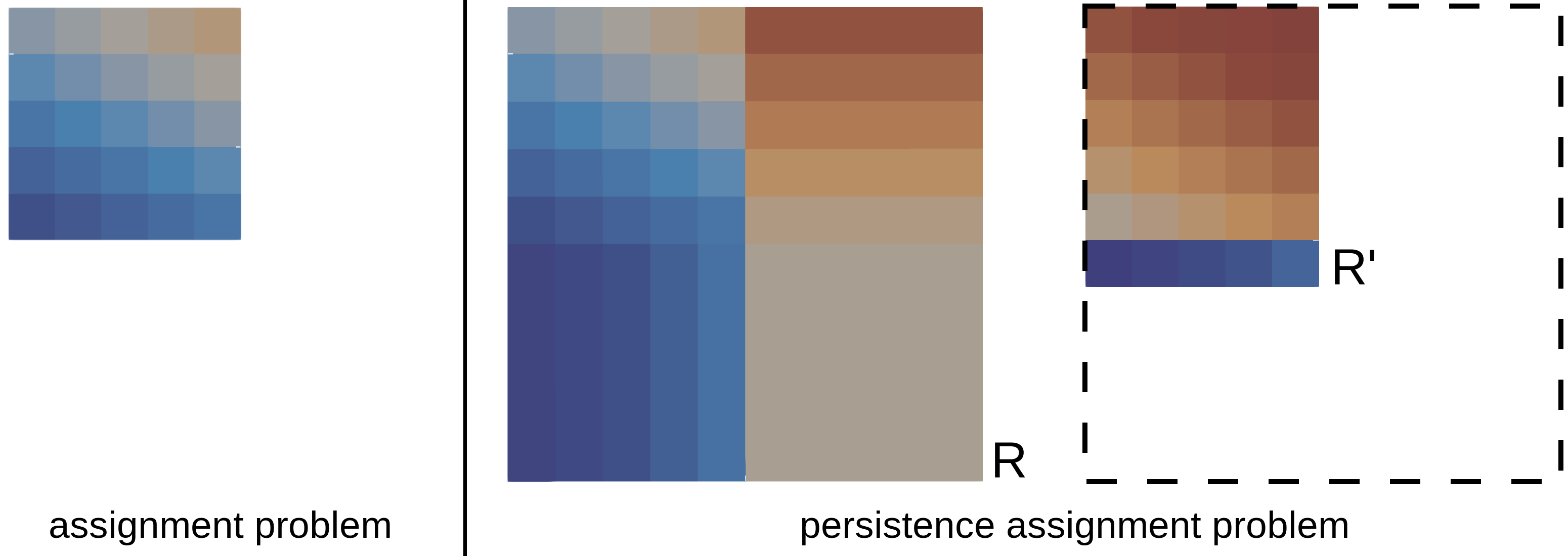
Figure 4: Cost matrices for a balanced assignment problem (left, $n\times n$ elements); for a persistence assignment problem with [50] (center, $R$ with $2n\times 2n$ elements – Eq. 3); and for the same persistence assignment problem with our proposed approach (right, $R^{\prime}$ with $(n+1)\times n$ elements – Eq. 4). Persistence elements in $R$ induce two redundant non-sparse blocks (top-right and bottom-left).

As a reminder, the original algorithm proceeds iteratively in two alternating phases: matrix reduction that makes new zeros appear, and augmenting path that finds a maximal set of independent zeros. At the $i^{th}$ iteration, the current maximal set of independent zeros is made of starred zeros. After a matrix reduction, new zeros appeared that can potentially belong to the new maximal set of independent zeros. Such candidates are primed. A single augmenting path (as in Fig. 3) replaces a set of $n$ starred zeros with $n+1$ primed zeros, forming a new set of independent zeros with one more element. Rows and columns of the matrix are marked as covered to restrict the search for candidates in the augmenting path phase. Blue blocks of Algorithm 1 indicate our extension of the Kuhn-Munkres algorithm.

In this novel extension, an augmenting path constructed in the corresponding phase can start from a starred zero in the last row (and then potentially find a primed zero in its column), but such a path can never access a starred zero in the last row at another step, for the corresponding column would have been covered prior to this (and thus cannot contain a primed zero, see Algorithm 1). A starred zero in the last row can then never be unstarred.

The Kuhn-Munkres approach has the property to only increase row values (and only decrease column values). When our algorithm working on the reduced matrix $R^{\prime}$ ends, it is therefore not possible that the elements on the top-right corner of the corresponding full matrix $R$ be negative. Furthermore, given Theorem 1, the resulting matrix corresponds to the same assignment problem.

2.2 Optimality

Working with the reduced matrix $R^{\prime}$, however, does not necessarily yield an optimal assignment. When assignments are found in the bottom row, if there has been additions to the matrix rows, then the corresponding $R$ matrix would contain a top-right block that is not zero, and a top-left block that is not zero either. Thus, the stop criterion stated by Theorem 2 may not be respected when $k=\min(m,n)$ lines are covered (as the real number of independent zeros in $R$ is $m+n$). Moreover, in our setup, a starred zero in the last column can never be unstarred; this is allowed in the approach on $R$, owing to the bottom-right block, initially filled with zeros.

Figure 5: In our setup, every element in the last row is considered independent, so that it can contain multiple starred zeros (left). This emulates the behavior of the bottom-left matrix block in the classical approach. During an $\epsilon$-reduction phase (center), we keep track of the (always positive) quantities that were added to matrix rows, hence increasing the top-right block in the classical approach, initially filled with only zeros. If a zero is starred in the last row and $j^{th}$ column, let $\rho_{i}$ be the sum of quantities added to row $i$ throughout the algorithm (right). If for all $i$, $r_{ij}>\rho_{i}$, then the persistence pair associated with column $i$ is assigned to the diagonal. If not (which never happened in our experiments), row residuals $\rho_{i}$ and the equivalent residuals for columns $\rho_{j}$ are used to report the partial optimization onto the matrix of the exact classical approach.

We therefore use the criterion stated in Eq. 5 to ensure that if, at any given iteration of the algorithm, a zero is starred in the last row of column $j$, the cost of assigning the corresponding persistence pair to any other pair is higher than the cost of leaving both unassigned (0 for the $j^{th}$-column pair and the residual value $\rho_{i}$ for $i^{th}$-row pairs – see Algorithm 1). This specificity is illustrated in Fig. 5.

$$\forall i\in\llbracket 0,n\rrbracket,r_{i,j}>\rho_{i}\Rightarrow r_{n+1,j}=0^{*}$$ (5)

The Eq. 5 criterion is checked whenever a zero appears on the last row after a subtraction is performed on a column by the algorithm. If it is observed, the corresponding column is removed from the problem and the persistence pair is set unassigned.

If the criterion is not respected, we have to report back the reduced problem onto the full matrix (missing banned columns and with reported found residuals $\rho$). For this, we need to keep track of residuals, that is, values that have been added or subtracted from each row and column throughout the course of the algorithm. Once these residuals have been reported onto the full matrix, there can be no negative element, and all of the optimization work has been reported (so that we do not start all over again from the beginning, but we start from the optimized output of the first phase).

In practice for persistence diagrams, we always observed that the first phase is sufficient to find an optimal assignment. Using this approach prevents from working with two potentially large blocks of persistence elements, typically occurring with the complete matrix for $i\in\llbracket n+1,m+n\rrbracket$ and $j\in\llbracket m+1,m+n\rrbracket$. This property is further motivated by the use of geometrical lifting (Sec. 3). The approach is detailed in Algorithm 1.

Data: $R^{\prime}=(r_{ij})$, an cost matrix,

Result: $S$ a set of starred independent zeros

$\forall i,\rho_{i}\leftarrow 0$ // row residuals

$\forall j,\rho_{j}\leftarrow 0$ // column residuals

$B\leftarrow\emptyset$ // banned columns

Subtract the persistence element from every row and $\rho_{i}$

Transpose $R^{\prime}$ if $n>m$ and let $k=\min(m,n)$

Subtract the min element from every of $R^{\prime}$

Star independent zeros and cover their columns

while number of covered columns $<k$ do

       Find a non-covered zero $Z_{1}$ and prime it

       if  there is no 0* in its row then

             Augmenting path phase (Fig. 3)

             Erase all primes, reset all covers

             Cover each column of containing a starred zero

            

      else

             Let $Z_{1}^{\prime}$ be the 0* in the row of $Z_{1}$

             Cover this row and uncover the column of $Z_{1}^{\prime}$

            

       end if

      if there is no uncovered zero left then

             Matrix $\epsilon$-reduction phase (Fig. 2)

             $\rho_{i}\leftarrow\rho_{i}+\epsilon$ for modified rows $i$

             $\rho_{j}\leftarrow\rho_{j}-\epsilon$ for modified columns $j$

             if $\exists j|r_{n+1,j}=0$ and $\forall i\in\llbracket 1,n\rrbracket,r_{i,j}>\rho_{i}$  then

                   $r_{n+1,j}$ is starred

                   $B\leftarrow B\cup j$

                  

             end if

            

       end if

      

end while

if $\exists j\notin B|r_{n+1,j}=0^{*}$ and $\exists i|r_{i,j}<\rho_{i}$ then

       Kuhn-Munkres($R_{ij}^{\prime\prime}=R_{ij}+\rho_{i}+\rho_{j}$) with $j\notin B$.

end if

Algorithm 1 Our algorithm for sparse persistence matching. Blue sections allow to emulate the behavior of the three original non-sparse blocks on one single row, while ensuring optimality thanks to the residuals column. Black sections are common with the unbalanced Kunk-Munkres algorithm.

2.3 Sparse assignment

In practice, it is often observed that some assignments are not possible, and that reordering columns in the associated cost matrix would enable faster lookups and modifications [18], using sparse matrices. With persistence diagrams, the following simple criterion (Eq. 6) can be used to discard lookups for potential matchings.

$$d_{\nu}(p,q)>d_{\nu}(p,\text{diag}(p))+d_{\nu}(q,\text{diag}(q))$$ (6)

Working with our version of the Kuhn-Munkres algorithm then becomes interesting for many assignments verify Eq. 6 (Fig. 6), hence greatly reducing the lookup time for zeros, minimal elements, and the access time for operations performed on rows or columns.

On the contrary, the original full-matrix version of Kuhn-Munkres deals with non-sparse blocks which have to be accessed and modified constantly throughout the course of the algorithm.

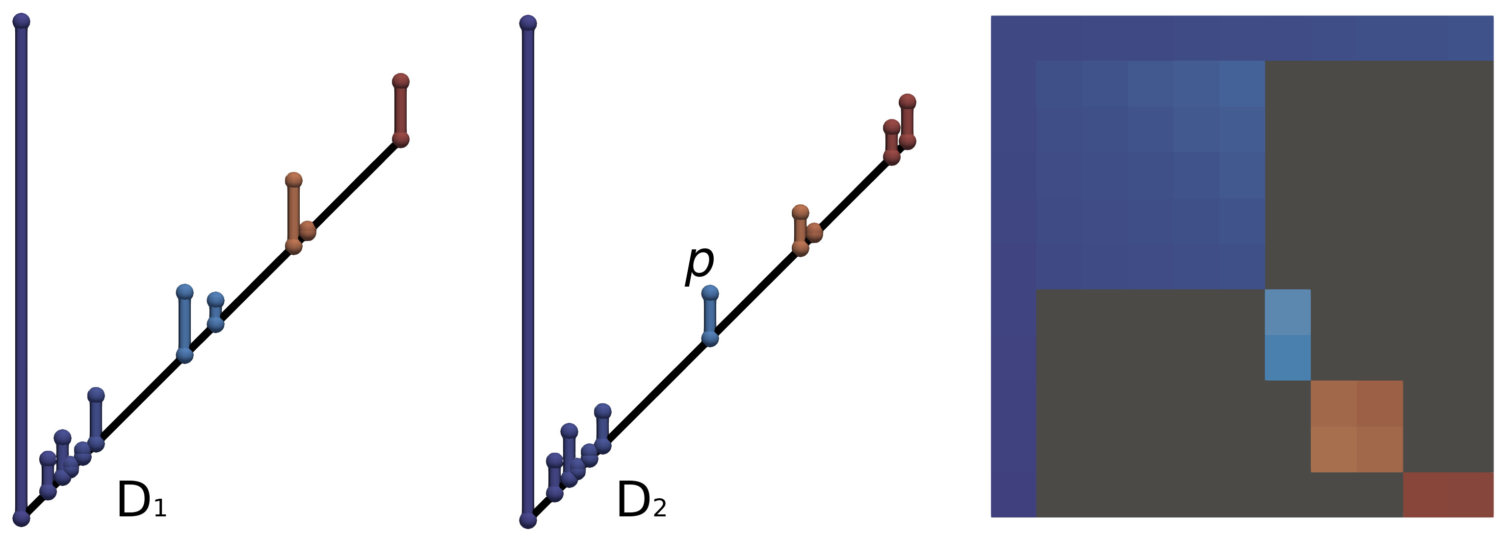
Figure 6: Persistence diagrams $D_{1}$ and $D_{2}$ showing in color small persistence pairs that will never be assigned in an optimal matching. The light blue pair $p\in D_{2}$ is such that $d(p,\text{diag}(p))+d(q,\text{diag}(q))<d(p,q)$ for any $q\in D_{1}$ which is neither light blue nor the first large persistence pair. This results in the cost matrix (right, $D_{1}$ pairs are rows and $D_{2}$ pairs are columns), where gray elements correspond to pairs $(p,q)$ s.t. $d(p,q)>d(p,\text{diag}(p))+d(q,\text{diag}(q))$.

Figure 7: Scalar field $f$ with persistence diagram $D(f)$ (left), matched with a scalar field $g$ with a similar persistence diagram $D(g)$, but an embedding that swaps the position of the light blue pair with that of the dark blue pair. Matched pairs are displayed with the same color using the non-geometric (center) and geometric Wasserstein metric (right). The latter takes the geometrical embedding into account, preventing similar pairs (regarding persistence) to be assigned if they are geometrically distant.

3 Lifted persistence Wasserstein metric

This section highlights the limitations of the natural Wasserstein metric applied to time-varying persistence diagrams and presents an extension that enhances its geometrical stability. Geometrical considerations are motivated, in terms of accuracy and performance.

Persistence diagrams can be embedded into the geometrical domain (Fig. 1). Doing so, one easily sees how different embeddings can correspond to similar persistence diagrams in the birth-death space. Working in this 2D space does yield irrelevant matchings: as can be seen in Fig. 7, when only the birth-death coordinates of persistence pairs are considered, a matching can be optimal even if it happens between geometrically distant zones. As a consequence, the distance metric between persistence pairs must be augmented with geometrical considerations.

To address this, we propose instead of $d_{\nu}$ (Eq. 1) to use the distance defined in Eq. 7:

$$d_{lift,\nu}(p,q)=(\alpha\delta_{birth}^{\nu}+\beta\delta_{death}^{\nu}+\gamma_{1}\delta_{x}^{\nu}+\gamma_{2}\delta_{y}^{\nu}+\gamma_{3}\delta_{z}^{\nu})^{1/\nu}\\$$ (7)

where $\delta_{x}$, $\delta_{y}$ and $\delta_{z}$ correspond to geometric distances between the extrema involved in the persistence pairs on a given axis. We process diagonal projections as follows (Eq. 8):

$$\begin{split}d_{lift,\nu}(p,\text{diag}(p))=&(\alpha\left|p_{x}\right|^{\nu}+\beta\left|p_{y}\right|^{\nu}+\\ &\gamma_{1}(\delta_{x}^{p})^{\nu}+\gamma_{2}(\delta_{y}^{p})^{\nu}+\gamma_{3}(\delta_{z}^{p})^{\nu})^{1/\nu}\end{split}$$ (8)

where the terms $\delta_{x}^{p}$, $\delta_{y}^{p}$ and $\delta_{z}^{p}$ correspond to the geometric distance between the critical points of a given pair $p$. Intuitively, it accounts for the distance between the critical points to cancel.

A lifted distance is considered by augmenting the geometric distance with coefficients $\alpha,\beta,\gamma_{i}$. This aims at giving more or less importance to the birth, death or some of the $x,y,z$ coordinates during the matching, depending on applicative contexts. For instance, in practice it is desirable to give less importance to the birth coordinate when dealing with $d$-$(d-1)$ persistence pairs (in other words, for tracking local maxima, see Fig. 8). For the remainder of the paper and the experiments, we used $(\alpha,\beta,\gamma_{i})=(0.1,1,1)$ for maxima and $(\alpha,\beta,\gamma_{i})=(1,0.1,1)$ for minima, for normalized geometrical extent and scalar values. We observed that using a lifted metric further increases the cost matrix sparsity, resulting in extra speedups.

Figure 8: Lifting the birth coordinate. 2D scalar fields with two gaussians (a, b), where the bottom (resp. top) gaussian has the maximum value (a) (resp. b). Using the geometrical metric alone (c) is not sufficient, as the birth coordinate $p_{x}$ misleadingly equalizes the persistence term of pairs of the same color in (a, b): $\delta_{p,yellow}^{a}=\delta_{p,yellow}^{b}$, $\delta_{p,blue}^{a}=\delta_{p,blue}^{b}$, potentially overcoming the geometrical factor. Lifting the birth coordinate with a small coefficient for associating maxima yields the correct matching (d).

Figure 9: Overview of our tracking approach on a dataset consisting of eight whirling gaussians: persistence diagram computations for two consecutive timesteps (a) and (b); matching of persistence pairs of two timesteps (c), propagation of matchings and construction of a trajectory (d).

4 Feature tracking

This section describes the four main stages of our tracking framework, relying on the discussed theoretical setup. Without loss of generality, we assume that the input data is a time-varying 2D or 3D scalar field defined on a PL-manifold. Topological features are extracted for all timesteps (Fig. 9, a-b), then matched (Fig. 9, c); trajectories are built from the successive matchings (Fig. 9, d) and post-processed to detect merging and splitting events.

4.1 Feature detection

First, we compute persistence diagrams for each timestep. We propose using the algorithm by Gueunet et al. [31], in which only $0$-$1$ and $d$-$(d-1)$ persistence pairs are considered.

When the data is noisy, it is possible to discard pairs of low persistence (typically induced by noise) by applying a simple threshold. In practice, this amounts to only considering the most prominent features. Using such a threshold accelerates the matching process, where for approaches based on overlaps, removing topological noise would require a topological simplification of the domain (for example using the approach in [86]), which is computationally expensive.

4.2 Feature matching

If $P_{1},P_{2}$ are two sets of persistence pairs taken at timesteps $t$ and $t+1$, then we use the algorithm described in Sec. 2, with the appropriate distance metric, as discussed in Sec. 3, to associate pairs in $P_{1}$ and $P_{2}$. A given pair $p_{1}\in P_{1}$ might be associated to one pair $p_{2}\in P_{2}$ at most, or not associated, and symmetrically.

4.3 Trajectory extraction

Trajectories are constructed by simply attaching successively matched segments. For all timesteps $t$, if the feature matching associates $p_{i}$ with $M_{t}(p_{i})=q_{j}$, then a segment is traced between $q_{j}$ and $p_{i}$, and is potentially connected back to the previous segment of $p_{i}$’s trajectory. If $M_{t}(p_{i})=\text{diag}(p_{i})$, the current trajectory ends. Properties are associated to trajectories (time span, critical point index) and to trajectory segments (matching cost, scalar value, persistence value, embedded volume).

4.4 Handling merging and splitting events

Given a user-defined geometrical threshold $\epsilon$, we propose to detect events of merging or splitting along trajectories in the following manner. If $T_{1},T_{2}:I\subset\mathbb{N}\rightarrow\mathbb{R}^{3}$ are two trajectories spanning throughout $[t_{i},t_{i+n}]$ and $[t_{j},t_{j+m}]$ respectively, and if for some $k\in[i,i+n]\cap[j,j+m]$, $d_{lift,\nu}(T_{1}(t_{k}),T_{2}(t_{k}))<\epsilon$, where $d_{lift,\nu}$ is a lifted distance, then an event of merging (or splitting) is detected. We consider that a merging event occurs between $T_{1}$ and $T_{2}$ at time $k$, when neither $T_{1}$ nor $T_{2}$ start at $t_{k}$. We then consider that the oldest trajectory takes over the youngest. For example, $T_{1}$ and $T_{2}$ meet (according to the $\epsilon$ criterion) at $t_{k}$ the last timestep of $T_{2}$, and $T_{2}$ started before $T_{1}$, then we disconnect the remainder of $T_{1}$ from the trajectory before $t_{k}$ and we connect it so as to continue $T_{2}$ until $T_{1}$’s original end. Similarly, a splitting event occurs between $T_{1}$ and $T_{2}$ at time $k$, when neither $T_{1}$ nor $T_{2}$ end at $t_{k}$. The process is illustrated in Fig. 10. It is done separately for distinct critical point types: minima, maxima and saddles are not mixed.

Figure 10: Merging process. Tracking is performed on two gaussians moving from left to right (a). The post-process detects a merging event with a geometrical threshold, then propagates the component identifier of the oldest component (b) and properly reconnects the matching segment. If the oldest component has already the right identifier (c) nothing is done. This process is proposed by analogy with building persistence diagrams.

5 Results

This section presents experimental results obtained on a desktop computer with two Xeon CPUs (3.0 GHz, 4 cores each), with 64 GB of RAM. We report experiments on 2D and 3D time-varying datasets, that were either simulated with Gerris [55] (von Kármán Vortex street, Boussinesq flow, starting vortex), or acquired (Sea surface height, Isabel hurricane). Persistence diagrams are computed with the implementation of [31] available in the Topology ToolKit [84]; the tracking is restricted to $0$-$1$ and $(d-1)$-$d$ pairs. We implemented our matching (Sec. 2) and tracking approaches (Sec. 4) in C++ as a Topology ToolKit module.

5.1 Application to simulated and acquired datasets

Figure 11: Sea surface height (SSH) captured over 365 days, 1 timestep every day. Local maxima are tracked in the region corresponding to the Agulhas Current, near South Africa (a); it is observed they are slowly drifting towards the west. SSH maxima are also drifting west in the less contrasted zone of the West Australian Current (b). Tracking in the region of the Kuroshio Current, near Japan (c), demonstrates a whirling behavior of local maxima.

Figure 12: Boussinesq flow generated by a heated cylinder (a). Feature tracking is performed (b) on the fluid vorticity. Some vortices exist over a long period of time (c), as others vanish more rapidly (d), sometimes akin to noise (e). Feature trajectories can easily be filtered from their lifespan.

Figure 13: Tracking performed on the wind velocity on a 3D Isabel hurricane dataset before (left), and after (right) temporal downsampling (1 frame every 5 timesteps). The global maximum is tracked successfully despite the high instability displayed by the scalar field.

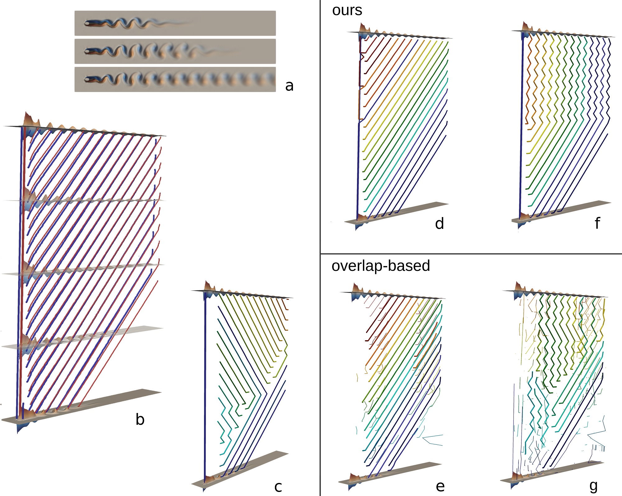
Figure 14: Simulated von Kármán vortex street (a), on which minima and maxima of the vorticity are tracked with our approach and 1% persistence filtering (b). Only taking the geometry and scalar value into account while doing the matchings (i.e. completely ignoring the birth in the lifted metric), is not sufficient to correctly track features (c). Maxima only are tracked considering 1 frame every 5 timesteps (d). With the same temporal resolution, the overlap-based approach (e) does capture small trajectories corresponding to noise, displayed with thinner lines, that have to be filtered for instance using topological simplification [86]. Considering 1 frame every 7 timesteps (f) still yields correct trajectories up to the point where, every other frame, optimal matchings for the metric are between a feature and the preceding one, due to features traveling fast. The overlap approach (g) is less stable in this case as it extracts erroneous trajectories from the very first stages of the simulation to the end.

We applied our tracking framework to both simulated and acquired time-varying datasets to outline specific phenomena.

In Fig. 11, we present the results of the tracking framework applied to an oceanographic dataset. The scalar field (sea surface height) is defined on 365 timesteps on a triangular mesh. We can see interesting trajectories corresponding to well-known oceanic currents. Drifting (a, b) and turbulent behaviors (c) of local extrema are highlighted. In Fig. 12, tracking is performed on the vorticity of highly unstable Boussinesq flow. Thanks to our analysis, trajectories can be filtered according to their temporal lifespan, revealing clearly different trajectory patterns among the turbulent features. This kind of analysis may be easily performed based on other trajectory attributes, depending on applicative contexts. In Fig. 13, we show our approach on a 3D hurricane dataset whose temporal resolution is such that a method based on overlaps of split-tree leaves (see Sec. 5.3) could not extract trajectories. In Fig. 14, our tracking framework correctly follows local extrema of the vorticity field in a simulated vortex street.

5.2 Tracking robustness

In the following two sections, we demonstrate the robustness and performance of our tracking framework.

We compare to the greedy approach based on the overlap of volumes [9, 8, 75, 66] of split-tree leaves, which amounts to tracking local maxima. In this approach, for every pair of consecutive timesteps $(t,t+1)$, split-tree segmentations $S_{t}$ and $S_{t+1}$ are computed (these are a set of connected regions). Overlap scores are then computed for every pair of regions $(s_{i},s_{j})\in S_{t}\times S_{t+1}$, as the number of common vertices between $s_{i}$ and $s_{j}$. Scores are sorted and $s_{i}$ is considered matched to the highest positive scoring $s_{j}$ such that $s_{j}$ has not been matched before. Trajectories are extracted by repeating the process for all timesteps.

Figure 15: Lifted Wasserstein tracking performed on a set of whirling 2D gaussians (a). With noise accounting for 10% of the scalar range (b), feature trajectories are still correctly detected. For 25% noise (c), 75% of the features (namely, the 6 most prominent out of the initial 8) are still correctly tracked despite heavy perturbations.

The robustness of our tracking framework is first assessed on a synthetic dataset consisting of whirling gaussians, on which we applied noise (Fig. 15). Identified trajectories are sensibly the same with a perturbation of 10% of the scalar range. The 75% most important features are still correctly tracked after a 25% random perturbation has been applied to the data.

In Fig. 14, our method is compared to the greedy approach, based on overlaps, while decreasing the temporal resolution. The overlap approach yields trajectories corresponding to noise (Fig. 14-e), which can be filtered by applying topological simplification beforehand (this would have a significant computational cost as it requires to modify the original function), or by associating the scalar value of the function to every point in the trajectory and then filtering the trajectory in a post-process step. In our setup, is is much simpler to discard this noise, by using a threshold for discarding small persistence pairs before the matching (implying a faster matching computation). When downsampling the temporal resolution to only 20% of the timesteps, our approach still gives the correct results (Fig. 14, d vs. e). With 15% of the timesteps, our approach (Fig. 14-f) still agrees with the tracking on the full-resolution data (Fig. 14-b), until preceding features begin to catch up, resulting in a zig-zag pattern. By comparison, the overlap method fails to correctly track meaningful regions from the beginning of the simulation to its end; it is indeed dependent on the geometry of overlaps, which is unstable. It can be argued that the locality captured by overlaps is emulated in our framework by embedding and lifting the Wasserstein metric, when the overlap method does not take persistence into account when matching regions. Also note that if the saddle component of persistence pairs associated to maxima is ignored (i.e. if $\alpha=0$ in Eq. 7 and Eq. 8) during the matching, then the geometrical distance can be insufficient for correctly tracking these persistence pairs (c). Therefore, the problem of matching persistence pairs for tracking topological features cannot be reduced to the (unbalanced) problem of assigning critical points in 4 dimensions (3 for the geometrical extent, one for the scalar value).

Fig. 13 further illustrates the robustness of our approach when downsampling the data temporal resolution. In hurricane datasets, local maxima can be displaced to geometrically distant zones between timesteps if those are taken at multiple-day intervals. This unstable behavior and the absence of obvious overlaps makes it particularly difficult to track extrema; nevertheless, our framework managed to track them at a very low time-resolution.

5.3 Tracking performance

We then compare our framework with our implementation of the approach based on overlaps [8] on the ground of performance. Figures are given in Table 1. Note that our approach has the advantage of taking persistence diagrams as inputs, so it can be applied to unstructured or time-varying meshes, for which overlap computations are not trivial. Our approach is also relatively dimension-independent: though in 3D, computing overlaps is very time-consuming (Fig. 1-Isabel), the complexity of the Wasserstein matcher, which only takes embedded persistence diagrams as inputs, for a given number of persistence pairs is sensibly equivalent. For both Isabel and Sea surface height datasets, we applied a 4% persistence filtering on input persistence diagrams. As the experiments show, our approach is faster in practice than the overlap method with best-match search.

Table 1: Time performance comparison (CPU time in seconds) between the approach based on overlaps of volumes [8] and our lifted Wasserstein approach. Tracking is performed over 50 timesteps, on structured 2D (Boussinesq, Vortex street), structured 3D (Isabel), and unstructured 2D (Sea surface height) meshes. The pre-processing step (FTM) computes the topology of the dataset. The post-processing step extracts the tracking mesh, computes its attributes, and handles splitting and merging events. We observe a parallel speedup ranging from 4 to 6 for our approach on 8 threads (FTM and matching phases).

Data-set	Pre-proc (s)	Matching (s)		Post-proc
	FTM	[8]	ours	(s)
Boussinesq	116	75	18	4.7
Vortex street	45	23	18	2.8
Isabel (3D)	863	$>$3k	17	162
Sea height	568	N.A.	277	113

5.4 Matching performance

Next, we compare the performance of the matching method we introduced in Sec. 2 to two other state-of-the art algorithms.

Table 2: Time performance comparison between the state-of-the-art Munkres-based approach [90], and our modified sparse approach.

Data-set	Sizes of diagrams	Time (s)
		[90]	ours
Starting vortex	$473-489$	68.6	1.26
Isabel	$465-413$	72.2	3.58
Boussinesq	$1808-1812$	11.1k	102
Sea height	$1950-5884$	26.5k	155

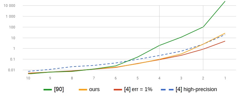
Figure 16: Running times in seconds of different matching approaches, for decreasing persistence thresholds expressed in percentage of the scalar range. The initial two diagrams containing 14,082 and 14,029 pairs are filtered to remove pairs whose persistence is less than the defined threshold, then a matching is computed with our new method, the reference exact method [90], the approximate method [4], first with 1% accuracy, then with an accuracy of $10^{-4}$% of the scalar range.

We compare it to the reference approach for the exact assignment problem [90] based on the Kuhn-Munkres algorithm, and to our implementation of the approximate approach based on the auction algorithm [4, 41], on the ground of performance.

Table 2 shows that our new assignment algorithm is up to two orders of magnitude faster than the classical exact approach [90]. In particular, the best speedups occur for the larger datasets which indicates that our approach also benefits from an improved scaling.

It is often useful in practice to discard low-persistence pairs prior to any topological data analysis as these correspond to noise. Fig. 16 compares the running times of our approach, [90] and [4] as more and more low-persistence pairs are taken into account. When removing pairs whose persistence is below 5% of the scalar range, which is commonly accepted as a conservative threshold, our approach is faster than all competing alternatives. When considering more low-persistence features, below 4%, our approach is competitive with the approximated auction approach with 1% error. Below 2%, only noise is typically added in the process. The performance of our algorithm becomes comparable to that of the high-precision auction approximation although our approach guarantees exact results.

5.5 Limitations

As we described, our framework enables the tracking of 0-1 and $d$-$(d-1)$ persistence pairs. It would be interesting to extend it to support the tracking of saddle-saddle pairs (in 3D) and see its application to meaningful use cases.

Besides, the lifting coefficients proposed in our metric (Eq. 7) might be seen as supplementary parameters that have to be tuned according to the dataset and applicative domain. Nonetheless, we observed in our experiments that these parameters do not require fine-tuning to produce meaningful tracking trajectories. The extent to which these can be enhanced by fine-tuning is left to future work.

The lifted distance can be generalized to take other parameters, such as the geometrical volume, mass, feature speed, into account, and be fine-tuned to answer the specificity of various scientific domains. Merging and splitting might also be enhanced, or given more flexibility, for instance with additional criteria. We also believe that the performance of the post-processing phase can be improved.

Additionally, we believe that the approximate auction algorithm can also take the lifted persistence metric into account by performing Wasserstein matchings between persistence pairs in 5 dimensions, and possibly benefit from geometry-based lookup accelerations, as suggested in lower dimension in [41]. It remains to be clarified how the quality of the matchings is affected in practice by using an approximate matching method, and how sparsity can enhance the research phase for the auction algorithm.

We note that the theoretical complexity of our matching method is, as the Munkres method, cubic; however, the two orders of magnitude speedups demonstrated in our experiments allow to study more challenging datasets. For very large case studies, the use of persistence thresholds could prove quite helpful for controlling the computing time of matchings. Among other non-trivial tracking methods, some graph matching methods are based on graph-edit distances [26, 1]. Their adaptation to the case of persistence diagrams or other topological structures (such as contour trees and Reeb graphs) may enable an additional structural regularization, this ought to be investigated in future work.

6 Conclusion

In this paper, we presented an original framework for tracking topological features in a robust and efficient way. It is the first approach combining topological data analysis and transport for feature tracking. As the kernel of our approach, we proposed a sparse-compliant extension of the seminal assignment algorithm for the exact matching of persistence diagrams, leveraging in practice important speedups. We introduced a new metric for persistence diagrams that enhances geometrical stability and further improves computation time. Overall, in comparison with overlap-based techniques, our approach displays improved performance and robustness to temporal downsampling, as experiments have shown.

We plan to release the implementation of our tracking framework open-source as a part of TTK [84] in the near future; we hope that it will be useful to the community with an interest for efficient tracking methods. We look forward to adapting it to tracking phenomena in in-situ contexts, where the large-scale time-varying data is accessed in a streaming fashion. As we are also interested in larger datasets, we are currently carrying out scaling tests on complex physical case studies available at Total S.A., for which one needs specifically adapted rendering techniques [47] to apprehend the resulting graphical complexity of the topology evolution.

We also believe that the application potential of our matching framework can be studied for tasks other than time-tracking, for instance, self-pattern matching and symmetry detection [82], or feature comparisons in ensemble data.

- [1] K. Beketayev, D. Yeliussizov, D. Morozov, G. H. Weber, and B. Hamann. Measuring the distance between merge trees. In Topological Methods in Data Analysis and Visualization III, pp. 151–165. Springer, 2014.
- [2] J. C. Bennett, H. Abbasi, P. T. Bremer, R. Grout, A. Gyulassy, T. Jin, S. Klasky, H. Kolla, M. Parashar, V. Pascucci, P. Pebay, D. Thompson, H. Yu, F. Zhang, and J. Chen. Combining in-situ and in-transit processing to enable extreme-scale scientific analysis. In High Performance Computing, Networking, Storage and Analysis (SC), 2012 International Conference for, pp. 1–9, Nov 2012.
- [3] D. P. Bertsekas. Network optimization: Continuous and discrete models, 1998.
- [4] D. P. Bertsekas and D. A. Castanon. The auction algorithm for the transportation problem. Ann. Oper. Res., 20(1-4):67–96, 1989.
- [5] S. Biasotti, D. Giorgio, M. Spagnuolo, and B. Falcidieno. Reeb graphs for shape analysis and applications. TCS, 2008.
- [6] A. Bock, H. Doraiswamy, A. Summers, and C. Silva. Topoangler: Interactive topology-based extraction of fishes. IEEE Transactions on Visualization and Computer Graphics, 24(1):812–821, Jan 2018.
- [7] F. Bourgeois and J.-C. Lassalle. An extension of the munkres algorithm for the assignment problem to rectangular matrices. Commun. ACM, 14(12):802–804, Dec. 1971.
- [8] P. Bremer, G. Weber, J. Tierny, V. Pascucci, M. Day, and J. Bell. Interactive exploration and analysis of large scale simulations using topology-based data segmentation. IEEE TVCG, 17(9):1307–1324, 2011.
- [9] P. T. Bremer, G. Weber, V. Pascucci, M. Day, and J. Bell. Analyzing and tracking burning structures in lean premixed hydrogen flames. IEEE Transactions on Visualization and Computer Graphics, 16(2):248–260, March 2010.
- [10] R. Burkard, M. Dell’Amico, and S. Martello. Assignment Problems. Society for Industrial and Applied Mathematics, Philadelphia, PA, USA, 2009.
- [11] H. Carr, J. Snoeyink, and U. Axen. Computing contour trees in all dimensions. Computational Geometry, 24(2):75–94, 2003.
- [12] H. Carr, J. Snoeyink, and M. van de Panne. Simplifying flexible isosurfaces using local geometric measures. In IEEE VIS, pp. 497–504, 2004.
- [13] M. Carrière, M. Cuturi, and S. Oudot. Sliced wasserstein kernel for persistence diagrams. In ICML, 2017.
- [14] F. Chazal, D. Cohen-Steiner, M. Glisse, L. J. Guibas, and S. Oudot. Proximity of Persistence Modules and their Diagrams. In SoCG, 2009.
- [15] D. Cohen-Steiner, H. Edelsbrunner, and J. Harer. Stability of persistence diagrams. In Symp. on Comp. Geom., pp. 263–271, 2005.
- [16] D. Cohen-Steiner, H. Edelsbrunner, and D. Morozov. Vines and vineyards by updating persistence in linear time. In Proceedings of the Twenty-second Annual Symposium on Computational Geometry, SCG ’06, pp. 119–126. ACM, New York, NY, USA, 2006.
- [17] D. A. S. C. A. Committee. Synergistic challenges in data-intensive science and exascale computing. Technical report, DoE Advanced Scientific Computing Advisory Committee, Data Sub-committee, 2013.
- [18] H. Cui, J. Zhang, C. Cui, and Q. Chen. Solving large-scale assignment problems by kuhn-munkres algorithm. In International Conference on Advances in Mechanical Engineering and Industrial Informatics (AMEII), 01 2016.
- [19] M. Cuturi. Sinkhorn distances: Lightspeed computation of optimal transport. In C. J. C. Burges, L. Bottou, M. Welling, Z. Ghahramani, and K. Q. Weinberger, eds., Advances in Neural Information Processing Systems 26, pp. 2292–2300. Curran Associates, Inc., 2013.
- [20] L. De Floriani, U. Fugacci, F. Iuricich, and P. Magillo. Morse complexes for shape segmentation and homological analysis: discrete models and algorithms. Comp. Grap. For., 2015.
- [21] H. Edelsbrunner and J. Harer. Jacobi sets of multiple morse functions. In Foundations of Computational Mathematics, 2004.
- [22] H. Edelsbrunner and J. Harer. Computational Topology: An Introduction. American Mathematical Society, 2009.
- [23] H. Edelsbrunner, J. Harer, A. Mascarenhas, and V. Pascucci. Time-varying reeb graphs for continuous space-time data. In Proceedings of the Twentieth Annual Symposium on Computational Geometry, SCG ’04, pp. 366–372. ACM, 2004.
- [24] H. Edelsbrunner, D. Letscher, and A. Zomorodian. Topological persistence and simplification. Disc. Compu. Geom., 28(4):511–533, 2002.
- [25] G. Favelier, C. Gueunet, and J. Tierny. Visualizing ensembles of viscous fingers. In IEEE SciVis Contest, 2016.
- [26] X. Gao, B. Xiao, D. Tao, and X. Li. A survey of graph edit distance. Pattern Analysis and applications, 13(1):113–129, 2010.
- [27] S. Grottel, G. Reina, J. Vrabec, and T. Ertl. Visual verification and analysis of cluster detection for molecular dynamics. IEEE Transactions on Visualization and Computer Graphics, 13(6):1624–1631, Nov 2007.
- [28] Y. Gu and C. Wang. Transgraph: Hierarchical exploration of transition relationships in time-varying volumetric data. IEEE Transactions on Visualization and Computer Graphics, 17(12):2015–2024, Dec 2011.
- [29] D. Guenther, R. Alvarez-Boto, J. Contreras-Garcia, J.-P. Piquemal, and J. Tierny. Characterizing molecular interactions in chemical systems. IEEE TVCG, 20(12):2476–2485, 2014.
- [30] C. Gueunet, P. Fortin, J. Jomier, and J. Tierny. Contour forests: Fast multi-threaded augmented contour trees. In IEEE LDAV, pp. 85–92, 2016.
- [31] C. Gueunet, P. Fortin, J. Jomier, and J. Tierny. Task-based augmented merge trees with Fibonacci heaps. In IEEE LDAV, 2017.
- [32] A. Gyulassy, P. T. Bremer, B. Hamann, and V. Pascucci. A practical approach to morse-smale complex computation: Scalability and generality. IEEE TVCG, 14(6):1619–1626, 2008.
- [33] A. Gyulassy, D. Guenther, J. A. Levine, J. Tierny, and V. Pascucci. Conforming morse-smale complexes. IEEE TVCG, 20(12):2595–2603, 2014.
- [34] A. Gyulassy, A. Knoll, K. Lau, B. Wang, P. Bremer, M. Papka, L. A. Curtiss, and V. Pascucci. Interstitial and interlayer ion diffusion geometry extraction in graphitic nanosphere battery materials. IEEE TVCG, 2015.
- [35] S. M. Hannon and J. A. Thomson. Aircraft wake vortex detection and measurement with pulsed solid-state coherent laser radar. Journal of Modern Optics, 41(11):2175–2196, 1994.
- [36] C. Heine, H. Leitte, M. Hlawitschka, F. Iuricich, L. De Floriani, G. Scheuermann, H. Hagen, and C. Garth. A survey of topology-based methods in visualization. Comp. Grap. For., 35(3):643–667, 2016.
- [37] G. Ji and H.-W. Shen. Efficient Isosurface Tracking Using Precomputed Correspondence Table. In O. Deussen, C. Hansen, D. Keim, and D. Saupe, eds., Eurographics / IEEE VGTC Symposium on Visualization. The Eurographics Association, 2004.
- [38] G. Ji and H.-W. Shen. Feature tracking using earth mover’s distance and global optimization. 2006.
- [39] G. Ji, H.-W. Shen, and R. Wenger. Volume tracking using higher dimensional isosurfacing. In Proceedings of the 14th IEEE Visualization 2003 (VIS’03), VIS ’03, pp. 28–, 2003.
- [40] L. Kantorovich. On the translocation of masses. AS USSR, 1942.
- [41] M. Kerber, D. Morozov, and A. Nigmetov. Geometry helps to compare persistence diagrams. J. Exp. Algorithmics, 22:1.4:1–1.4:20, Sept. 2017.
- [42] T. Klein and T. Ertl. Scale-space tracking of critical points in 3d vector fields. In H. Hauser, H. Hagen, and H. Theisel, eds., Topology-based Methods in Visualization, pp. 35–49. Springer Berlin Heidelberg, Berlin, Heidelberg, 2007.
- [43] H. W. Kuhn and B. Yaw. The hungarian method for the assignment problem. Naval Res. Logist. Quart, pp. 83–97, 1955.
- [44] A. Landge, V. Pascucci, A. Gyulassy, J. Bennett, H. Kolla, J. Chen, and T. Bremer. In-situ feature extraction of large scale combustion simulations using segmented merge trees. In SuperComputing, 2014.
- [45] D. E. Laney, P. Bremer, A. Mascarenhas, P. Miller, and V. Pascucci. Understanding the structure of the turbulent mixing layer in hydrodynamic instabilities. IEEE TVCG, 2006.
- [46] E. Levina and P. Bickel. The earthmover’s distance is the mallows distance: some insights from statistics. In IEEE ICCV, vol. 2, pp. 251–256, 2001.
- [47] J. Lukasczyk, G. Weber, R. Maciejewski, C. Garth, and H. Leitte. Nested tracking graphs. Comp. Graph. For., 36(3):12–22, 2017.
- [48] G. Monge. Mémoire sur la théorie des déblais et des remblais. Académie Royale des Sciences de Paris, 1781.
- [49] K. Moreland, R. Oldfield, P. Marion, S. Jourdain, N. Podhorszki, V. Vishwanath, N. Fabian, C. Docan, M. Parashar, M. Hereld, M. E. Papka, and S. Klasky. Examples of in transit visualization. In Proceedings of the 2Nd International Workshop on Petascal Data Analytics: Challenges and Opportunities, PDAC ’11, pp. 1–6. ACM, New York, NY, USA, 2011.
- [50] D. Morozov. Dionysus. http://www.mrzv.org/software/dionysus/, 2010.
- [51] J. Munkres. Algorithms for the assignment and transportation problems, 1957.
- [52] S. Ozer, D. Silver, K. Bemis, and P. Martin. Activity detection in scientific visualization. IEEE Transactions on Visualization and Computer Graphics, 20(3):377–390, March 2014.
- [53] V. Pascucci, G. Scorzelli, P. T. Bremer, and A. Mascarenhas. Robust on-line computation of Reeb graphs: simplicity and speed. ToG, 26(3):58, 2007.
- [54] V. Pascucci, X. Tricoche, H. Hagen, and J. Tierny. Topological Data Analysis and Visualization: Theory, Algorithms and Applications. Springer, 2010.
- [55] S. Popinet. Gerris: A tree-based adaptive solver for the incompressible euler equations in complex geometries. J. Comput. Phys., 190(2):572–600, 2003.
- [56] F. H. Post, B. Vrolijk, H. Hauser, R. S. Laramee, and H. Doleisch. The state of the art in flow visualisation: Feature extraction and tracking. Computer Graphics Forum, 22(4):775–792, 2003.
- [57] M. Rasquin, P. Marion, V. Vishwanath, B. Matthews, M. Hereld, K. Jansen, R. Loy, A. Bauer, M. Zhou, O. Sahni, J. Fu, N. Liu, C. Carothers, M. Shephard, M. Papka, K. Kumaran, and B. Geveci. Electronic poster: Co-visualization of full data and in situ data extracts from unstructured grid cfd at 160k cores. In Proceedings of the 2011 Companion on High Performance Computing Networking, Storage and Analysis Companion, SC ’11 Companion, pp. 103–104. ACM, New York, NY, USA, 2011.
- [58] G. Reeb. Sur les points singuliers d’une forme de Pfaff complètement intégrable ou d’une fonction numérique. Acad. des Sci., 1946.
- [59] F. Reinders, F. H. Post, and H. J. Spoelder. Visualization of time-dependent data with feature tracking and event detection. The Visual Computer, 17(1):55–71, Feb 2001.
- [60] J. Reininghaus, S. Huber, U. Bauer, and R. Kwitt. A stable multi-scale kernel for topological machine learning. In IEEE CVPR, 2015.
- [61] J. Reininghaus, J. Kasten, T. Weinkauf, and I. Hotz. Efficient computation of combinatorial feature flow fields. IEEE Transactions on Visualization and Computer Graphics, 18(9):1563–1573, 2012.
- [62] T. Ringler, M. Petersen, R. L. Higdon, D. Jacobsen, P. W. Jones, and M. Maltrud. A multi-resolution approach to global ocean modeling. Ocean Modelling, 69:211 – 232, 2013.
- [63] M. Rivi, L. Calori, G. Muscianisi, and V. Slavnic. In-situ visualization: State-of-the-art and some use cases. 2011.
- [64] K. Robbins, C. Jeffrey, and S. Robbins. Visualization of splitting and merging processes. Journal of Visual Languages and Computing, 11(6):593 – 614, 2000.
- [65] V. Robins, P. Wood, and A. Sheppard. Theory and algorithms for constructing discrete morse complexes from grayscale digital images. IEEE Trans. on Pat. Ana. and Mach. Int., 2011.
- [66] H. Saikia and T. Weinkauf. Global feature tracking and similarity estimation in time-dependent scalar fields. Comput. Graph. Forum, 36(3):1–11, June 2017.
- [67] R. Samtaney, D. Silver, N. Zabusky, and J. Cao. Visualizing features and tracking their evolution. Computer, 27(7):20–27, 1994.
- [68] K. Shi, H. Theisel, H. Hauser, T. Weinkauf, K. Matkovic, H.-C. Hege, and H.-P. Seidel. Path Line Attributes - an Information Visualization Approach to Analyzing the Dynamic Behavior of 3D Time-Dependent Flow Fields, pp. 75–88. Springer, 2009.
- [69] K. Shi, H. Theisel, T. Weinkauf, H. Hauser, H.-C. Hege, and H.-P. Seidel. Path line oriented topology for periodic 2D time-dependent vector fields. In Proc. Eurographics / IEEE VGTC Symposium on Visualization (EuroVis ’06), pp. 139–146. Lisbon, Portugal, May 2006.
- [70] D. Silver. Object-oriented visualization. IEEE Comput. Graph. Appl., 15(3):54–62, May 1995.
- [71] D. Silver and X. Wang. Volume tracking. In Visualization ’96. Proceedings., pp. 157–164, Oct 1996.
- [72] D. Silver and X. Wang. Tracking and visualizing turbulent 3d features. IEEE Transactions on Visualization and Computer Graphics, 3(2):129–141, Apr 1997.
- [73] D. Silver and X. Wang. Tracking scalar features in unstructured data sets. In Visualization ’98. Proceedings, pp. 79–86, Oct 1998.
- [74] D. Silver and X. Wang. Visualizing evolving scalar phenomena. Future Generation Computer Systems, 15(1):99 – 108, 1999.
- [75] B. S. Sohn and C. Bajaj. Time-varying contour topology. IEEE TVCG, 12(1):14–25, 2006.
- [76] J. Solomon, F. de Goes, G. Peyré, M. Cuturi, A. Butscher, A. Nguyen, T. Du, and L. J. Guibas. Convolutional wasserstein distances: efficient optimal transportation on geometric domains. ACM Trans. Graph., 34(4):66:1–66:11, 2015.
- [77] J. Solomon, G. Peyré, V. G. Kim, and S. Sra. Entropic metric alignment for correspondence problems. ACM Trans. Graph., 35(4):72:1–72:13, July 2016.
- [78] T. Sousbie. The persistent cosmic web and its filamentary structure: Theory and implementations. Royal Astronomical Society, 414(1):350–383, 2011.
- [79] H. Theisel and H.-P. Seidel. Feature flow fields. In Procs. of the Symp. on Data Visualisation 2003, VISSYM ’03, pp. 141–148. Eurographics Association, Aire-la-Ville, Switzerland, Switzerland, 2003.
- [80] H. Theisel, T. Weinkauf, H. C. Hege, and H. P. Seidel. Stream line and path line oriented topology for 2d time-dependent vector fields. In IEEE Visualization 2004, pp. 321–328, Oct 2004.
- [81] H. Theisel, T. Weinkauf, H. C. Hege, and H. P. Seidel. Topological methods for 2d time-dependent vector fields based on stream lines and path lines. IEEE Transactions on Visualization and Computer Graphics, 11(4):383–394, July 2005.
- [82] D. M. Thomas and V. Natarajan. Multiscale symmetry detection in scalar fields by clustering contours. IEEE TVCG, 2014.
- [83] J. Tierny and H. Carr. Jacobi fiber surfaces for bivariate Reeb space computation. IEEE TVCG, 23(1):960–969, 2016.
- [84] J. Tierny, G. Favelier, J. A. Levine, C. Gueunet, and M. Michaux. The Topology ToolKit. IEEE TVCG, 24(1):832–842, 2017.
- [85] J. Tierny, A. Gyulassy, E. Simon, and V. Pascucci. Loop surgery for volumetric meshes: Reeb graphs reduced to contour trees. IEEE TVCG, 15(6):1177–1184, 2009.
- [86] J. Tierny and V. Pascucci. Generalized topological simplification of scalar fields on surfaces. IEEE TVCG, 18(12):2005–2013, 2012.
- [87] X. Tricoche, T. Wischgoll, R. G. Scheuermann, and H. Hagen. Topology tracking for the visualization of time-dependent two-dimensional flows. Computers and Graphics, 26(2):249 – 257, 2002.
- [88] C. Villani. Optimal Transport: Old and New. Springer, 2009 ed., Sept. 2008.
- [89] C. Wang and J. Tao. Graphs in scientific visualization: A survey. Computer Graphics Forum, 36(1):263–287, 2017.
- [90] J. Weaver. An implementation of the kuhn–munkres algorithm. https://github.com/saebyn/munkres-cpp, 2013.
- [91] G. Weber, P.-T. Bremer, M. Day, J. Bell, and V. Pascucci. Feature Tracking Using Reeb Graphs, pp. 241–253. Springer Berlin Heidelberg, Berlin, Heidelberg, 2011.
- [92] W. Widanagamaachchi, J. Chen, P. Klacansky, V. Pascucci, H. Kolla, A. Bhagatwala, and P. T. Bremer. Tracking features in embedded surfaces: Understanding extinction in turbulent combustion. In 2015 IEEE 5th Symposium on Large Data Analysis and Visualization (LDAV), pp. 9–16, Oct 2015.
- [93] H. Yu, C. Wang, R. W. Grout, J. H. Chen, and K. L. Ma. In situ visualization for large-scale combustion simulations. IEEE Computer Graphics and Applications, 30(3):45–57, May 2010.
- [94] F. Zhang, E. Fiorelli, and N. E. Leonard. Exploring scalar fields using multiple sensor platforms: Tracking level curves. In 2007 46th IEEE Conference on Decision and Control, pp. 3579–3584, Dec 2007.
- [95] F. Zhang, S. Lasluisa, T. Jin, I. Rodero, H. Bui, and M. Parashar. In-situ feature-based objects tracking for large-scale scientific simulations. In 2012 SC Companion: High Performance Computing, Networking Storage and Analysis, pp. 736–740, Nov 2012.