A hierarchical statistical framework for emergent constraints: application to snow-albedo feedback

Abstract

Emergent constraints use relationships between future and current climate states to constrain projections of climate response. Here, we introduce a statistical, hierarchical emergent constraint (HEC) framework in order to link future and current climate with observations. Under Gaussian assumptions, the mean and variance of the future state is shown analytically to be a function of the signal-to-noise (SNR) ratio between data-model error and current-climate uncertainty, and the correlation between future and current climate states. We apply the HEC to the climate-change, snow-albedo feedback, which is related to the seasonal cycle in the Northern Hemisphere. We obtain a snow-albedo-feedback prediction interval of $(-1.25,-0.58)$ %$K^{-1}$. The critical dependence on SNR and correlation shows that neglecting these terms can lead to bias and under-estimated uncertainty in constrained projections. The flexibility of using HEC under general assumptions throughout the Earth System is discussed.

Geophysical Research Letters

Jet Propulsion Laboratory, California Institute of Technology, Pasadena, California, USA National Institute for Applied Statistics Research Australia (NIASRA), University of Wollongong, Australia Department of Atmospheric and Oceanic Sciences, University of California, Los Angeles, California, USA.

K.W.Bowmankevin.bowman@jpl.nasa.gov ©2018. All rights reserved.

A hierarchical emergent constraints (HEC) framework for climate projections is introduced.

HEC depends on the signal-to-noise ratio between observational and climate uncertainty.

Using HEC, the snow-albedo-feedback prediction interval is found to be $(-1.25,-0.58)$ %$K^{-1}$.

1 Introduction

The confrontation of predictions with observations as a means of testing theories is a key demarcation of science and critical to the advancement of scientific knowledge (Popper, 1959). In fields such as numerical weather prediction, data assimilation techniques provide a mathematical framework for narrowing the range or uncertainty of predictions through repeated evaluation against a broad suite of observations (Tarantola, 2006; Lewis et al., 2006). Reducing the uncertainty in climate projections has been one of the signature challenges in Earth science. In contrast to weather forecasting, the time scales of climate projections do not permit ready validation. While historic and current observations can be used to benchmark climate models (e.g., Gleckler et al., 2008; Teixeira et al., 2014), the establishment of robust relationships between contemporary performance and the credibility in future response has proven difficult. One of the primary techniques to explore these relationships is through climate-model ensembles (Collins, 2007). These ensembles may be derived from a core model where “parametric” uncertainty is explored using, inter alia, perturbed physics ensemble experiments (e.g., Allen et al., 2000; Murphy et al., 2004). Other approaches exploit ensembles from the Coupled Model Intercomparison Project (CMIP) (Taylor et al., 2011; Eyring et al., 2016) or similar MIPs in order to represent “structural” uncertainty (Yokohata et al., 2013), which is the result of different physical representations of processes. These are used in weighting schemes that aim to provide the “best” combination of models rather than a strict model democracy (e.g., Tebaldi et al., 2005; Smith et al., 2009). The “emergent” or “observational” constraint approach, as a means of using observations to indirectly reduce the uncertainty in climate projections, has only recently been appreciated (e.g., Collins, 2007; Collins et al., 2012; Klein and Hall, 2015; Cox et al., 2018).

Here, an emergent constraint (EC) is composed of

1. A dependence between future climate, $z_{t+\tau}$, and current climate, $x_{t}$.

2. A dependence between observations, $y_{t}$, and current climate, $x_{t}$.

Here, these dependencies will be expressed in terms of correlation. It is the synthesis of these quantities that yields an EC. For simplicity, “current” climate also refers to historic climate. Generally, a regression between future climate and current climate is calculated empirically from a climate-model ensemble. Through this relationship, model projections correlated with current-climate simulations but inconsistent with observations should be treated with additional caution. These inconsistencies can signal where more focused research is warranted (e.g., DeAngelis et al., 2015).

The EC approach has been applied to regional and global climate studies (e.g., Hall and Qu, 2006; Fasullo and Trenberth, 2012; Qu and Hall, 2014; Sherwood et al., 2014; Borodina et al., 2017; Cox et al., 2018) and more broadly for Earth System studies (e.g., Cox et al., 2013; Bowman et al., 2013; Wenzel et al., 2016). These studies compute correlations between $z_{t+\tau}$ and $x_{t}$ where they identify the range of models whose $x_{t}$ are within the precision of the observations, $y_{t}$. However, they do not combine these factors to compute an estimate of future climate. For example, Fasullo and Trenberth (2012) show that the relative humidity (RH) in the dry descending branch of circulation (300-500 hPa at 15^∘) of most climate models is biased high in RH with respect to observations. Models with high RH also tend to have lower equilibrium climate sensitivity (ECS). However, this study did not provide a quantitative method to incorporate the present-future climate correlation ($-0.81$ in their case), the bias between observations and ensemble mean, and the observation uncertainty into an estimate of ECS, thereby limiting the study to qualitative conclusions. Cox et al. (2018) provide a quantitative, probabilistic framework to estimate ECS given observations and current climate, however their formulation does not include an explicit description of observational uncertainty. This manuscript is careful to distinguish between $y_{t}$ and $x_{t}$ providing a framework that explicitly incorporates each of these critical elements of EC.

Here, we approach ECs from a hierarchical statistical modeling perspective (e.g., Cressie and Wikle, 2011). The relationship between observations, states or processes, and parameters, are related through conditional probability distributions. Bayes’ Theorem is employed to obtain a predictive distribution for these states given the observations. This framework allows us to give a prescriptive approach that integrates both model and observational uncertainties. Moreover, it has inherent recursive properties through conditional distributions that subsume data assimilation algorithms such as Kalman filtering, which are implemented in various forms in numerical weather prediction (e.g. Kalman, 1960; Navon, 2009; Wikle and Berliner, 2007). This approach has been applied to climate analysis, including regional-climate prediction and climate-change detection and attribution (Kang and Cressie, 2013; Katzfuss et al., 2017).

The hierarchical emergent constraint (HEC) framework introduced here explicitly relates future climate, current climate, and observations through conditional-probability distributions that allow us to generalize previous EC studies. For the purpose of illustration, we assume all distributions are Gaussian and develop analytical formulas for these conditional distributions. This simplification allows for a direct comparison to the EC literature where the Gaussian assumption is implicit. We then illustrate our approach by comparing the HEC to the “classic” EC (CEC) for the snow-albedo feedback of Hall and Qu (2006), updated to use Climate Model Intercomparison Project-5 (CMIP5) models (Taylor et al., 2011; Qu and Hall, 2014). The physical processes relating the current seasonal cycle and the future snow-albedo feedback are fairly straightforward, leading to a causal interpretation of the correlative relationship between future and current climate  (Klein and Hall, 2015). The HEC is subsequently used to explore how the correlation of the future and current climate and the observational uncertainty (expressed through a signal-to-noise ratio) impact future climate-change estimates. Challenges and future directions for this approach are discussed in the concluding section.

2 Methods

2.1 Hierarchical statistical framework for emergent constraints

A general probabilistic model of emergent constraints is based upon the joint probability distribution of the future and current climate given the observations, which can be written as follows:

$$[z_{t+\tau},x_{t}|y_{t}]\equiv\frac{[z_{t+\tau},x_{t},y_{t}]}{\int[z_{t+\tau},x_{t},y_{t}]dx_{t}dz_{t+\tau}},$$ (1)

where $z_{t+\tau}$, $x_{t}$, and $y_{t}$ are random variables (or random vectors) representing the future climate, the current climate, and the observations, respectively. The bracket notation, $[x]$, represents the probability density function of the variable $x$, and $[x|y]$ is the conditional probability density function of $x$ given $y$ (Cressie and Wikle, 2011). The time indices, $t$ and $t+\tau$, ($\tau$¿0) are used notationally to distinguish between the current and future state. The term “current” refers to both contemporary and historic states, or observations. For simplicity, these variables are referred to as states but can also be referred to as processes (e.g., snow-albedo feedback). The conditional density in Equation 1 can be represented as:

$$[z_{t+\tau},x_{t}|y_{t}]=[z_{t+\tau}|x_{t}][x_{t}|y_{t}],$$ (2)

since $[z_{t+\tau}|x_{t},y_{t}]=[z_{t+\tau}|x_{t}]$. That is, the conditional distribution of future climate is independent of observations when the current climate is already known. The future climate $z_{t+\tau}$ is predictable given $x_{t}$, if $[z_{t+\tau}|x_{t}]\neq[z_{t+\tau}]$ (DelSole and Tippett, 2007). Current climate $x_{t}$ is observable if the observations $y_{t}$ satisfy $[x_{t}|y_{t}]\neq[x_{t}]$.

A hierarchical emergent constraint (HEC) can be defined as the probability of the future state given observations of the current state; that is,

$$[z_{t+\tau}|y_{t}]=\int[z_{t+\tau}|x_{t}][x_{t}|y_{t}]dx_{t},$$ (3)

since $[z_{t+\tau}|y_{t}]$ is obtained as a marginal distribution of Equation 1. An EC defined by Equation 3 leads to a slightly different interpretation than the operational definition used in Cox et al. (2018), which is generally focused on $[z_{t+\tau}|x_{t}]$. This difference can be critical when the data-model error on $y_{t}$ given $x_{t}$ is large. That is, $[y_{t}|x_{t}]$ needs to be accounted for, as does knowledge of $x_{t}$, leading to an appropriate $[x_{t}|y_{t}]$ on the right-hand side of Equation 3. As we demonstrate below, a weak correlation between $z_{t+\tau}$ and $x_{t}$ can be partially offset by a strong correlation between $y_{t}$ and $x_{t}$ (i.e., how well the climate is observed), and vice versa. Consequently, the predictability and observability of climate are inextricably linked.

The inference of $x_{t}$ from observations, $y_{t}$, frequently use Bayesian techniques (e.g., Rodgers, 2000):

$$[x_{t}|y_{t}]=\frac{[y_{t}|x_{t}][x_{t}]}{[y_{t}]}.$$ (4)

As will be shown in the next section, $[x_{t}|y_{t}]$ accounts for the uncertainty of the observing system (data-model errors) and the uncertainty of the state (state error). Substitution of Equation 4 into Equation 3 leads to

$$[z_{t+\tau}|y_{t}]=\frac{1}{[y_{t}]}\int[z_{t+\tau}|x_{t}][y_{t}|x_{t}][x_{t}]dx_{t}.$$ (5)

The distributions inside the integral of Equation 5 are typically straightforward, but the denominator, $y_{t}$, can be problematic to compute. However, when Gaussian assumptions are made, it has an analytical form and can be evaluated easily.

2.2 Application to linear Gaussian constraints

ECs in the literature frequently express the relationship between the future and current state in terms of a simple linear regression. These regressions can in turn be interpreted as the first moment of a conditional density of Gaussian distributions. In the leading case where $z_{t+\tau}$, $x_{t}$, and $y_{t}$ are jointly Gaussian, a closed-form expression for [$z_{t+\tau}|y_{t}$] can be obtained analytically.

Assume that the observations are related to current climate through

$$y_{t}=x_{t}+n_{t},$$ (6)

where $x_{t}\sim\mathcal{N}(\mu_{x_{t}},\sigma^{2}_{x_{t}})$ and $n_{t}\sim\mathcal{N}(0,\sigma^{2}_{n_{t}})$ are independent Gaussian random variables parameterized by their mean and variance. The observation, $y_{t}$, is a measurement of the true climate state, $x_{t}$, and the error, $n_{t}$, which incorporates multiple sources of uncertainty including systematic and random error from the measurement along with representation and model error (Brasseur and Jacob, 2017). There may be bias in the error, which would lead to a non-zero mean. If the bias can be determined, then it can be subtracted from the observation, $y_{t}$, in Equation 6.

Combining Equation 6 with Equation 4, we obtain

$$[y_{t}|x_{t}][x_{t}]\propto\exp\left[-\frac{(y_{t}-x_{t})^{2}}{2\sigma^{2}_{n_{t}}}\right]\exp\left[-\frac{(x_{t}-\mu_{x_{t}})^{2}}{2\sigma^{2}_{x_{t}}}\right].$$ (7)

Then, the Maximum A Posteriori (MAP) estimate of $x_{t}$ is the expectation of the conditional distribution in Equation 4, which can be calculated from Equation 7 to be

$$E(x_{t}|y_{t})=\mu_{x_{t}}+K_{x_{t},y_{t}}(y_{t}-\mu_{x_{t}}),$$ (8)

and the conditional variance is

$$var(x_{t}|y_{t})=(1-K_{x_{t},y_{t}})\sigma^{2}_{x_{t}},$$ (9)

where

$$K_{x_{t},y_{t}}=\frac{\sigma^{2}_{x_{t}}}{\sigma^{2}_{x_{t}}+\sigma^{2}_{n_{t}}}.$$ (10)

The quantity $K_{x_{t},y_{t}}$ is the “gain” of the MAP estimator, which balances the uncertainty in the current state with the precision of the observation (Wikle and Berliner, 2007).

Under our assumptions, $z_{t+\tau}$ and $x_{t}$ are jointly Gaussian. Consequently, the future climate state conditioned on the current state is

$$E(z_{t+\tau}|x_{t})=\mu_{z_{t+\tau}|x_{t}} = \mu_{z_{t+\tau}}+K_{z_{t+\tau},x_{t}}(x_{t}-\mu_{x_{t}})$$ (11)

$$var(z_{t+\tau}|x_{t})=\sigma^{2}_{z_{t+\tau}|x_{t}} = \sigma^{2}_{z_{t+\tau}}-K^{2}_{z_{t+\tau},x_{t}}\sigma^{2}_{x_{t}}=(1-\rho^{2})\sigma^{2}_{z_{t+\tau}},$$ (12)

where

$$K_{z_{t+\tau},x_{t}}=\frac{\rho\sigma_{z_{t+\tau}}}{\sigma_{x_{t}}},$$ (13)

and $\rho$ is the correlation coefficient between $z_{t+\tau}$ and $x_{t}$. The expectation in Equation 11 can be cast as a simple “straight-line” approximation between these states, namely, $z_{t+\tau}=\alpha+\beta x_{t}$, where $\beta=K_{z_{t+\tau},x_{t}}$ is the slope, and $\alpha=\mu_{z_{t+\tau}}-K_{z_{t+\tau},x_{t}}\mu_{x_{t}}$ is the intercept. It is this ”straight-line” approximation in ECs that is fitted from climate-model ensembles.

Equations 8–9 and 11–12 define up-to-second-order statistical descriptions of the current state given observations, (i.e., $[x_{t}|y_{t}]$) and the future state given the current state, (i.e., $[z_{t+\tau}|x_{t}]$). Under Gaussian assumptions, all conditional densities $[z_{t+\tau}|x_{t}]$, $[x_{t}|y_{t}]$, and $[z_{t+\tau}|y_{t}]$ are Gaussian, and hence only their first and second moments are needed.

The derivations that follow up to Equation 24, do not require Gaussian assumptions. Applying the law of iterated expectations (Ross, 2010), the first moment of $[z_{t+\tau}|y_{t}]$ is

$$E(z_{t+\tau}|y_{t})=E(E(z_{t+\tau}|y_{t},x_{t}))=E(E(z_{t+\tau}|x_{t})|y_{t}).$$ (14)

Substituting Equation 11 into Equation 14, yields

$$E(z_{t+\tau}|y_{t})=\mu_{z_{t+\tau}}+K_{z_{t+\tau},x_{t}}(E(x_{t}|y_{t})-\mu_{x_{t}}).$$ (15)

Equation 8 can then be substituted into Equation 15, yielding:

$$E(z_{t+\tau}|y_{t})=\mu_{z_{t+\tau}|y_{t}} = \mu_{z_{t+\tau}}+K_{z_{t+\tau},x_{t}}K_{x_{t},y_{t}}(y_{t}-\mu_{x_{t}})$$ (16)

$$= \mu_{z_{t+\tau}}+\frac{\rho\sigma_{z_{t+\tau}}\sigma_{x_{t}}}{\sigma^{2}_{x_{t}}+\sigma^{2}_{n_{t}}}(y_{t}-\mu_{x_{t}}).$$ (17)

Defining the statistically normalized anomaly of the future-climate estimate, $\delta_{z_{t+\tau}|y_{t}}\equiv(\mu_{z_{t+\tau}|y_{t}}-\mu_{z_{t+\tau}})/\sigma_{z_{t+\tau}}$ and the normalized anomaly of the current-climate estimate, $\delta_{x_{t}|y_{t}}\equiv(y_{t}-\mu_{x_{t}})/\sigma_{x_{t}}$, Equation 17 can be rearranged to yield

$$\frac{\delta_{z_{t+\tau}|y_{t}}}{\delta_{x_{t}|y_{t}}}=\frac{\rho}{1+(\sigma^{2}_{x_{t}}/\sigma^{2}_{n_{t}})^{-1}}.$$ (18)

The magnitude of the normalized update is driven by $\rho$ and $(\sigma^{2}_{x_{t}}/\sigma^{2}_{n_{t}})$. The first term is the correlation between the future and current climate, and the second quantity is

$$\mathrm{SNR}\equiv\frac{\sigma^{2}_{x_{t}}}{\sigma^{2}_{n_{t}}},$$ (19)

which defines the relative strength of the signal variability to the noise variability. If the signal dominates the noise, then the update of the anomaly ratio in Equation 18 is controlled by $\rho$. Conversely, if noise dominates then, as expected, the forecast anomaly will be close to zero. Notice that the normalized anomaly in the future climate estimate $z_{t+\tau}$ is proportional to $\rho$. For $\rho=1$, the update in Equation 18 is controlled by the SNR and, for $\rho=0$, no update is zero.

In order to calculate the variance (the central second moment of $[z_{t}|y_{t}]$) of the EC, the law of total variance (e.g., Ross, 2010) is invoked:

$$var(z_{t+\tau}|y_{t})=E(var(z_{t+\tau}|x_{t})|y_{t})+var(E(z_{t+\tau}|x_{t})|y_{t}).$$ (20)

By substituting Equations 9, 11, and 12 into the right-hand side of Equation 20, the variance of the HEC can be written as

$$var(z_{t+\tau}|y_{t})=\sigma^{2}_{z_{t+\tau}|y_{t}} = var(z_{t+\tau}|x_{t})+K^{2}_{z_{t+\tau},x_{t}}var(x_{t}|y_{t})$$ (21)

$$= \sigma^{2}_{z_{t+\tau}}-K^{2}_{z_{t+\tau},x_{t}}K_{x_{t},y_{t}}\sigma^{2}_{x_{t}}$$ (22)

$$= \left(1-\frac{\rho^{2}}{1+(\sigma^{2}_{x_{t}}/\sigma^{2}_{n_{t}})^{-1}}\right)\sigma^{2}_{z_{t+\tau}}$$ (23)

The right-hand side of Equation 23 can be normalized to compute a relative reduction in variance:

$$\frac{\sigma^{2}_{z_{t+\tau}|y_{t}}}{\sigma^{2}_{z_{t+\tau}}}=\left(1-\frac{\rho^{2}}{1+(\sigma^{2}_{x_{t}}/\sigma^{2}_{n_{t}})^{-1}}\right),$$ (24)

which is always between 0 and 1.

Under Gaussian assumptions, Equations 17 and 23 provide a complete description of the dependence of the future climate’s distribution given the observations, $y_{t}$, of the current climate. There are some important limiting conditions that illuminate the relationships between future climate, current climate, and observations. Similar to Equation 18, the change in uncertainty is driven by the interplay between $\rho$ and the SNR. As $\rho\rightarrow 0$, then $[z_{t+\tau}|y_{t}]$ converges in distribution to $[z_{t+\tau}]$, which is expected. That is, if observations are uncorrelated with the future state, they will have no impact on the uncertainty of that state. If the SNR is high (i.e., $\sigma^{2}_{x_{t}}>>\sigma^{2}_{n_{t}}$), then the relative reduction in the uncertainty of the future state is controlled completely by the correlation through $1-\rho^{2}$, and the CEC coincides with the HEC we have developed here.

3 Application to snow-albedo feedback

The snow-albedo feedback (SAF) is an important component of the global hydrological response to increases in carbon dioxide (Bony et al., 2006). The SAF accounts for much of the spread in Northern Hemispheric (NH) landmass warming (Qu and Hall, 2014). This feedback amplifies global and NH warming since snow-cover retreat accelerates when mean temperatures increase, which exposes a lower albedo surface that in turn leads to a decrease in net shortwave (SW) radiation, $\bar{Q}_{\mathrm{net}}$, at the top-of-the-atmosphere (TOA). The SAF-induced change in $\bar{Q}_{\mathrm{net}}$ to surface temperature can be expressed as

$$\frac{\Delta\bar{Q}_{\mathrm{net}}}{\Delta\bar{T}_{s}}=-\frac{1}{A_{R}}\int_{S,R}Q(t,r)\frac{\partial\alpha_{p}}{\partial\alpha_{s}}(t,r)\frac{\Delta\alpha_{s}}{\Delta\bar{T}_{s}}(t)dtdr,$$ (25)

where $Q(t,r)$ is the incoming radiation at TOA at time $t$ and position $r$, $\alpha_{p}$ is the planetary albedo, $\alpha_{s}$ is the surface-albedo, $A_{R}$ is the area of region $R$, $\Delta\bar{T}_{s}$ is a change in the regionally averaged surface air temperature, and the domains of integration are the annual cycle, $S$, and a region $R$. Annually, $\Delta\bar{Q}_{\mathrm{net}}$ is controlled in part by the magnitude of the snow-albedo sensitivity to temperature, which is $\Delta\alpha_{s}(t)/\Delta\bar{T}_{s}(t)$, especially during the NH Spring. The sensitivity, which is a function of snow cover and vegetation type, is climate-model dependent. Qu and Hall (2014) showed that there is a strong correlation between climate models with a large sensitivity and their change in NH landmass temperatures through the snow-albedo feedback.

In order to diagnose the snow-albedo feedback in climate models, $\Delta\overline{\alpha}^{sc}_{s}$ and $\Delta\overline{T}^{sc}_{s}$ are defined as the difference between April and May surface albedo and temperature, respectively, averaged over NH extratropical landmasses. Their ratio, $\Delta\overline{\alpha}^{sc}_{s}/\Delta\overline{T}^{sc}_{s}$, is the seasonal cycle snow-albedo temperature sensitivity (SCSAT). Likewise, $\overline{\alpha}^{cc}_{s}$ and $\Delta\overline{T}^{cc}_{s}$ are quantified by the difference in April values between the current (1980–1999) and future (2080–2099) climates regionally averaged over NH extratropical landmasses. Their ratio is the climate-change snow-albedo temperature sensitivity (CCSAT).

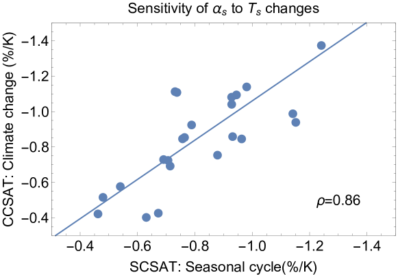
Figure 1: Linear regression of the climate-change snow-albedo temperature (CCSAT) against the seasonal cycle snow-albedo temperature sensitivity (SCSAT) defined over Northern Hemispheric land. Each of the 25 dots represents a CMIP5 model computed in Qu and Hall (2014).

Figure 1 shows the regression between CCSAT and SCSAT across 25 CMIP5 models. The regression is characterized by a strong correlation ($\rho$ = 0.86) along with a slope (1.11) and intercept (0.05 $\%K^{-1}$) that are close to unity and zero, respectively. The correlation here reflects a physical relationship defined through Equation 25. Consequently, the SAF in the contexts of both seasonal cycle (current) and climate change (future) is similarly influenced by these physically related processes (Qu and Hall, 2014).

Applying the HEC framework to SAF, we define $x_{t}=\Delta\overline{\alpha}^{sc}_{s}/\Delta\overline{T}^{sc}_{s}$, which is SCSAT and $z_{t+\tau}=\overline{\alpha}^{cc}_{s}/\Delta\overline{T}^{cc}_{s}$, which is CCSAT. Figure 2 shows the spread of the SCSAT as a Gaussian probability density function estimated from the CMIP5 models and is denoted as $[x_{t}]$. Qu and Hall (2014) showed that the model-spread in the seasonal cycle is attributable to the mean effective snow albedo, which in turn is controlled primarily by land-surface modeling (e.g., vegetation canopy). The CMIP5 SCSAT first-order and (square root) second-order moments are $\mu_{x}=-0.860~{}\%K^{-1}$ and $\sigma_{x}=0.244~{}\%K^{-1}$, respectively. Consequently the variability is about 30% of the absolute mean.

An observational constraint on SCSAT is based upon a combination of MODIS surface-albedo measurements from 2001–2012 (Jin et al., 2003) and surface air temperature from ERA-interim (Dee et al., 2011). We refer the interested reader to Qu and Hall (2014) for additional details. The observed SCSAT is $y_{t}=-0.87$ %K^-1 with an observational uncertainty of $\sigma_{n_{t}}=0.04$ %K^-1. Consequently, the one-standard-deviation range is $[-0.92,-0.83]$ %K^-1. Figure 2 shows the observationally constrained distribution calculated from Equations 8 and 9. The conditional mean is $\mu_{x_{t}|y_{t}}=-0.870$ %K^-1, and the conditional uncertainty is $\sigma_{x_{t}|y_{t}}=0.0395$ %K^-1. Hence, $\sigma_{x_{t}|y_{t}}$ is about 6 times less than $\sigma_{x_{t}}$,the uncertainty in the unconditional distribution of the state $x_{t}$.

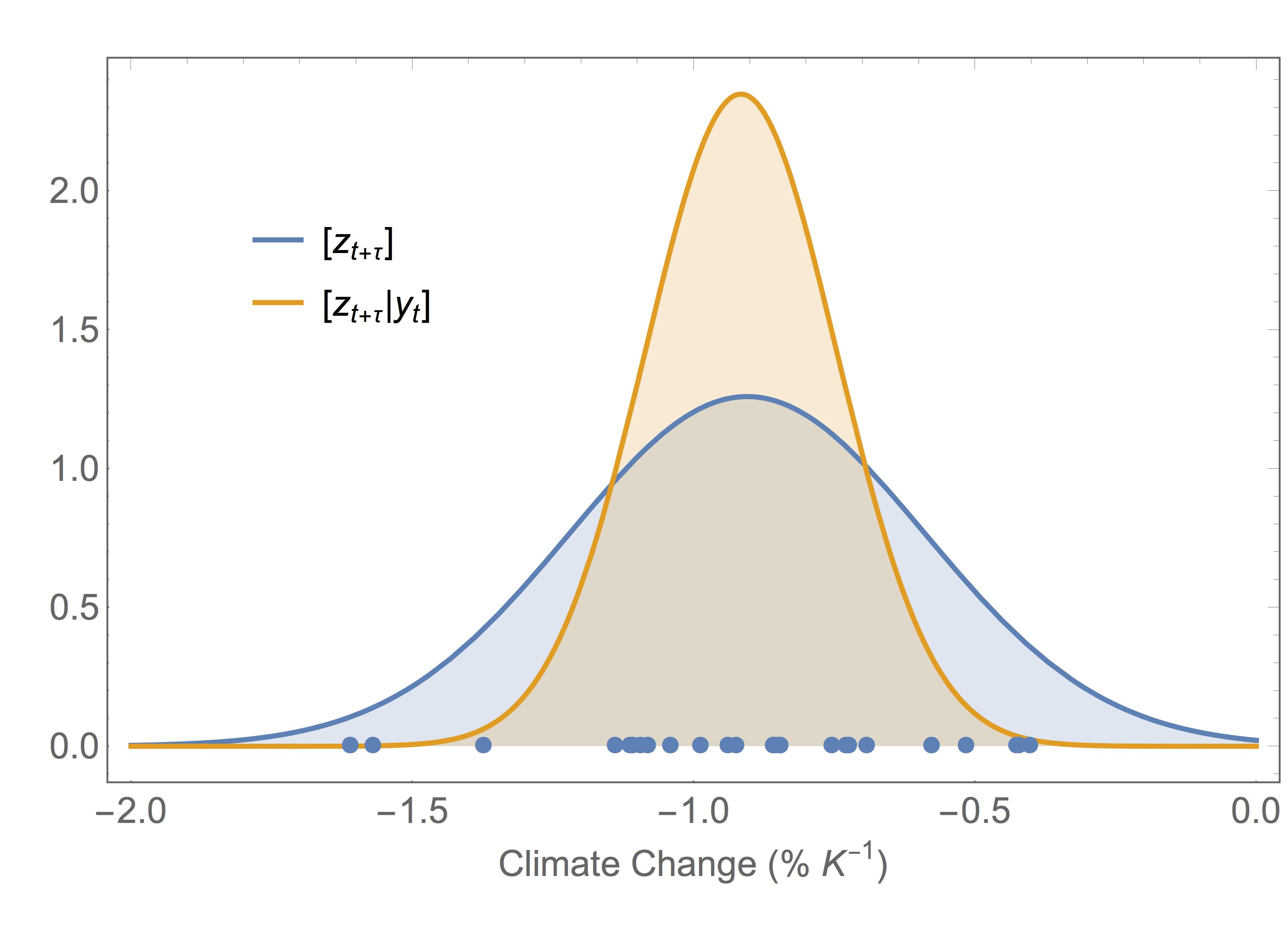
Figure 3: The fitted Gaussian probability density functions (pdf) of climate-change snow-albedo temperature sensitivity (CCSAT), which is defined as the ratio of the change in snow-albedo in April between present day (1980-1999) and future (2080-2099) normalized by the change in regionally averaged NH land temperatures averaged over the same time periods. Individual model estimates of the CCSAT are represented by dots along the abscissa.

The effects of observations on the predictive distribution of CCSAT is the critical question, which was not addressed in Qu and Hall (2014). It would be tempting to simply use the regression line itself to project the observational estimate of SCSAT into CCSAT. However, that would neglect the critical role of $\rho$ and SNR. The HEC of CCSAT, $[z_{t+\tau}|y_{t}]$, is shown in Figure 3 and computed from Equation 3 assuming jointly Gaussian distributions with a conditional mean (computed from Equation 17) to be $\mu_{z_{t+\tau}|y_{t}}=-0.916$ %$K^{-1}$, and the conditional uncertainty (computed from Equation 23) to be $\sigma_{z_{t+\tau}|y_{t}}=0.170$ %$K^{-1}$. The conditional mean is similar to the mean of the state, $\mu_{z_{t+\tau}}=-0.905$ %K^-1, but the conditional uncertainty, $\sigma_{z_{t+\tau}|y_{t}}$ is about 1.9 times less than $\sigma_{z_{t+\tau}}$ = 0.317 %K^-1. This is seen from Equation 24 where the role of $\rho=0.86$ and SNR=$(6.1)^{2}$ is crucial here.

The HEC can now be used to obtain the predictive distribution of CCSAT given observations, which goes beyond the results in Hall and Qu (2006) and Qu and Hall (2014). Based on the marginal distribution $[x_{t}]$ from the CMIP5 models, the 95% prediction interval of CCSAT is $(-1.425,-0.385)$ %$K^{-1}$. With HEC, the 95% prediction interval has narrowed substantially to $(-1.25,-0.58)$ %$K^{-1}$.

4 Role of the signal-to-noise ratio and correlation in HEC

The snow-albedo feedback provides a good starting point to consider HEC in a broader context. The analytical solution shows that in a normalized form (Equations 18 and 24), the conditional mean and the conditional variance in the update are a function of only the correlation $\rho$ and the SNR. Increases in $\rho$ and SNR both act in the HEC to reduce the uncertainty in future climate. To explore these two mechanisms, Figures 4 and 5 show the normalized conditional mean update (Equation 18) and the normalized uncertainty reduction factor (Equation 24) resulting from the use of the HEC. The black circles in those figures are computed based upon $\rho$=0.86 and $\sqrt{\mathrm{SNR}}=6.1$ obtained for the SAF study.

A one standard deviation anomaly for both the normalized CCSAT and SCSAT is unity. The the right-hand side of Equation 18 is the weight that scales the CCSAT anomaly ($\delta_{z_{t+\tau}|y_{t}}$) relative to the SCSAT anomaly ($\delta_{x_{t}|y_{t}}$). For a perfect correlation and high SNR, the weight itself is nearly unity; a normalized anomaly in CCSAT is equal to a normalized anomaly in SCSAT ($\delta_{z_{t+\tau}|y_{t}}/\delta_{x_{t}|y_{t}}\approx 1$). The range of weights is shown in Figure 4 where the black dot is on the 0.83 contour corresponding to ($\rho$, $\sqrt{\mathrm{SNR}}$)=(0.86, 6.1) for this study. Figure 5 shows the contour plot of the reduction factor in the variance (i.e., $\sigma^{2}_{z_{t+\tau}|y_{t}}/\sigma^{2}_{z_{t+\tau}}$ from Equation 24) for CCSAT; the black dot is on the 0.29 contour again corresponding to ($\rho$, $\sqrt{\mathrm{SNR}}$)=(0.86, 6.1). It is important to note that this reduction is not unique to the SAF study. Any HEC with the same correlation and SNR will yield a variance reduction of approximately 30%. For a hypothetical HEC with the same correlation as the SAF, but a much smaller SNR of 1, the normalized update would be reduced to $\rho/2$=0.43 (as compared to 0.83 in our case) and the variance reduction factor of $1-\rho^{2}/2=$ 0.8 (as compared to 0.54 in our case). This interplay, especially the role of observational uncertainty, is not found in the formulation of Cox et al. (2018). We have shown that neglecting the role of observational uncertainty, which is the case in classic EC, can lead to incorrect prediction intervals especially for lower precision data such as those discussed in Fasullo and Trenberth (2012) and Sherwood et al. (2014).

5 Conclusions

Projections of change in the Earth System from anthropogenic forcing is one of the defining challenges in climate science. ECs represent an important approach to incorporating observations into climate-model projections that relate present-day variability to future response. In this work, ECs are explicitly defined through Equation 3 as conditional distributions within a HEC framework. Classical EC studies frequently use a linear regression but do not account for both the correlation between $z_{t+\tau}$ and $x_{t}$ and the precision in observing $x_{t}$ with $y_{t}$ as does HEC. The formulation of the Maximum A Posterior (MAP) solution in Equation 17 more directly links EC with data assimilation techniques. For non-Gaussian processes, more advanced tools such as Markov Chain Monte Carlo (MCMC) could be used to compute accurate prediction intervals based on the HEC (Cressie and Wikle, 2011).

Like any statistical approach, assessing whether $[z_{t+\tau}|x_{t}]$ is causal remains an important challenge (Klein and Hall, 2015). While this work does not explicitly address these considerations, the HEC framework introduced here more readily allows EC to be linked to causality analysis (e.g. Pearl, 2009; Sugihara et al., 2012).

We note the joint distribution $[z_{t+\tau},x_{t}]$ is dependent on the climate-model ensemble, which may not be robust to model choice or may systematically miss important processes. Increased and systematic use of observations and high-resolution modeling can improve confidence in Earth-System models (Schneider et al., 2017), of which this approach can readily take advantage. Current applications of EC have generally used averaged scalar processes $z_{t+\tau}$, $x_{t}$, and $y_{t}$. Including multiple types of observations $y^{(1)}_{t}$, $y^{(2)}_{t}$, $\ldots$ sensitive to $x_{t}$ within this framework, will provide more information for implementing ECs from processes simulated in climate models. This is especially true for critical climate metrics such as the equilibrium climate sensitivity, which depends on multiple processes including water vapor, clouds, and snow-albedo feedbacks. We would expect that incorporating multiple measurements that are sensitive to a range of these key feedbacks will ultimately be necessary to constrain climate projections. That extension is a subject of future research.

Figure 2: The fitted Gaussian probability density functions (pdf) of seasonal cycle snow-albedo temperature sensitivity (SCSAT), which is defined as the ratio of the change in snow-albedo between May and June normalized by the change in temperature. Individual model-based estimates are represented by dots along the abscissa.

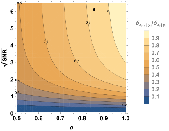
Figure 4: Normalized change in the predicted anomaly in the future state as a function of correlation ($\rho$) and signal-to-noise ratio (SNR). The black dot on the 0.83 contour is positioned at ($\rho$, $\sqrt{\mathrm{SNR}}$)=(0.86, 6.1) for the CMIP5 models and observations from Qu and Hall (2014).

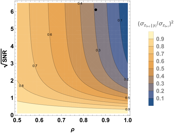
Figure 5: Normalized reduction factor as a function of correlation, $\rho$, and signal-to-noise ratio (SNR). The black dot on the 0.29 contour is the ($\rho$, $\sqrt{\mathrm{SNR}}$)=(0.86, 6.1) for the CMIP5 models and observations from Qu and Hall (2014).