Statistical analysis on XMM-Newton X-ray flares of Mrk 421: distributions of peak flux and flaring time duration

Abstract

The energy dissipation mechanism in blazar jet is unknown. Blazar’s flares could provide insights on this problem. Here we report statistical results of XMM-Newton X-ray flares of Mrk 421. We analyze all public XMM-Newton X-ray observations for Mrk 421, and construct the light curves. Through fitting light curves, we obtain the parameters of flare-profiles, such as peak flux ($F_{\rm p}$) and flaring time duration ($T_{\rm fl}$). It is found that both the distributions of $F_{\rm p}$ and $T_{\rm fl}$ obey a power-law form, with the same index of $\alpha_{\rm F}=\alpha_{\rm T}\approx 1$. The statistical properties are consistent with the predictions by a self-organized criticality (SOC) system with energy dissipation in one-dimensional space. This is similar to solar flare, but with different space dimensions of the energy dissipation domain. This suggests that X-ray flaers of Mrk 421 are possibly driven by a magnetic reconnection mechanism. Moreover, in the analysis, we find that variability on timescale of $\sim 1000\$s frequently appears. Such rapid variability indicates a magnetic field of $\geq 2.1\delta_{\rm D}^{-1/3}$ G ($\delta_{\rm D}$ is the Doppler factor) in emission region.

1 Introduction

Blazars are a rather extreme class of radio-loud active galactic nuclei (AGNs), consisting of BL Lac objects (BL Lacs) and flat-spectrum radio quasars (FSRQs). Due to relativistic Doppler boosting, blazar emission is dominated by the non-thermal emission coming from its jet. Its spectral energy distribution (SED) extends from radio to $\gamma$-rays, and shows two bumps. The low-energy bump is believed to be the synchrotron radiation of relativistic electrons, while the origin of high-energy bump is under debate. A variety of emission mechanisms are proposed to explain this origin: (1) inverse Compton (IC) scattering of low-energy photons by relativistic electrons, including synchrotron self-Compton model (i.e., SSC; e.g., Maraschi et al., 1992) and external Compton model (i.e., EC; e.g., Dermer & Schlickeiser, 1993; Sikora et al., 1994); (2) relativistic proton synchrotron radiation (Mannheim & Biermann, 1992; Aharonian, 2000; Mücke et al., 2003); (3) synchrotron radiation of secondary particles produced in proton-photon interaction (Mücke & Protheroe, 2001; Böttcher et al., 2009; Yan & Zhang, 2015; Cerruti et al., 2015) .

According to the peak frequency of synchrotron bump ($\nu_{\rm p}$), BL Lacs are divided into three classes (e.g., Padovani & Giommi, 1995): high-synchrotron-frequency peaked BL Lacs (HBLs; $\nu_{\rm p}>10^{15}\$Hz), intermediate-synchrotron-frequency peaked BL Lacs (IBLs; $10^{14}<\nu_{\rm p}<10^{15}\$Hz), and low-synchrotron-frequency peaked BL Lacs (LBLs; $\nu_{\rm p}<10^{14}\$Hz). FSRQs usually have $\nu_{\rm p}<10^{14}\$Hz.

Blazars show strong variability across entire electromagnetic emission on timescales from minutes to years (e.g., Aharonian et al., 2007; Dai et al., 2015; Ackermann et al., 2016; Zhu et al., 2018). Variability timescale can be used to constrain the size of emission region, the magnetic field in emission region, and the location of high energy emission region (e.g., Böttcher et al., 2003; Yan et al., 2018). The correlations of variabilities in different spectral bands could carry abundant information on the emission and acceleration mechanisms of particles in blazar jet (e.g., Fossati et al., 2008; Chen et al., 2016). Although variability is important and useful for understanding blazar jet physics, the physical origin of blazar variability is not well understood. Several scenarios have been proposed to understand the production of variability (see Aharonian et al., 2017, for a review), like magnetospheric gap model (e.g., Neronov & Aharonian, 2007), jet-star interaction model (e.g., Barkov et al., 2012), and jet-in-jet model (e.g., Giannios et al., 2009). Magnetic reconnection may play an important role in the latter two models (e.g., Aharonian et al., 2017). Sironi et al. (2015) argued that magnetic reconnection, rather than shock, powers blazar jet emission.

Statistical properties of flares could provide insights into the trigging mechanism of flares. The flares trigged by magnetic reconnection is thought to form a self-organized criticality (SOC) system, such as solar flares (e.g., Lu & Hamilton, 1991; Aschwanden, 2011). The SOC flare system expects that event parameters, e.g., the flux and the flaring time duration, should follow power-law distributions. The indices of these power laws are related to the effective geometric dimension of the system (e.g., Aschwanden, 2012). Such a statistical approach has been used to investigate whether the SOC model can explain the X-ray flares of $\gamma$-ray bursts (GRBs; Wang & Dai, 2013; Yi et al., 2016, 2017), M87 (Wang et al., 2015), and Sgr A^∗ (Wang et al., 2015; Li et al., 2015; Yuan et al., 2018). Here, we apply this approach to X-ray flares of Mrk 421.

Mrk 421 is a HBL. It is the brightest blazar in the X-ray sky. Its X-ray emission is believed to be the synchrotron radiation of relativistic electrons, showing strong and rapid variabilities (e.g., Cui, 2004; Fossati et al., 2008; Paliya et al., 2015; Kapanadze et al., 2016, 2018). The main goal of this paper is to investigate whether the statistical properties of Mrk 421 XMM-Newton X-ray flares are consistent with the expectations of a SOC system.

2 Data reduction

We search for the archived data of Mrk 421 in XMM-Newton Science Archive, and collect a total of 50 observations containing EPIC exposures. All the observational information are collected in Table 1. Following the standard procedures of the SAS threads, we reprocess the raw data files to obtain calibrated and concatenated event lists, using the SAS version 15.0.0. We then check flaring high background periods; and create clear event lists which are free of high background (namely the data is screened by a new good time interval), using the background count rate threshold of "RATE$<=$0.4" for PN data and "RATE$<=$0.35" for MOS data.

Before selecting the source regions, we check whether there are pile-up effects on the observations. It is found that most of the observations are affected by pile-up effects, as listed in Table 2 (column 10). To reduce the pile-up effects, we extract the light curves and spectra from core-excised regions. For image mode, the region is an annular area; for timing mode, each region is comprised of two columns. The selected source regions are listed in Table 2 (column 11). The background regions are extracted from the places near the source regions in the same event maps. Before the light curves and spectra extraction, we set the extracted event pattern and flag to be "FLAG==0 && PATTERN$<=$4" for all PN data, while "PATTERN$<=$12" for image mode MOS data and "FLAG ==0 && PATTERN==0" for timing mode MOS data. We create response matrix files and ancillary response files for the extracted spectra using the rmfgen and arfgen tasks. The spectra prepared for analysis are grouped in order to make sure that there are at least 20 counts for each spectral channel.

XSPEC (version 12.9) is used for spectral analysis. We use $\chi^{2}$ statistic in spectral fittings. We first separately apply a power-law, a broken power-law and a log-parabola models to data, to determine the best-fit model. We find that all the three models are failed to fit the spectra, with the reduced $\chi^{2}_{r}\gtrsim 2.0$. The log-parabola (LP) model is better than the others. Therefore, we determine the LP model as the basic component of a new model, and then try to add other components to reduce $\chi^{2}_{r}$. Ultimately, we find that a model containing a log-parabola and a black body (i.e., LP+BB) is the best-fit model for most of the spectra. In the fittings, we notice that there are some unknown line-shape humps in some spectra around 0.5 keV, resulting in a large $\chi^{2}_{r}$. We speculate that those phenomena are caused by out-of-time events. To eliminate this effect, we add Lorenz line (Lor) components in the models. All best-fitting parameters are given in Table 2. In all spectral fittings, the Galactic hydrogen absorption is considered. The Galactic hydrogen column density (N_H) is fixed to, by default, 1.92$\times$10²⁰ cm^-2 which is produced by Leiden/Argentine/Bonn (LAB) Survey (Kalberla et al., 2005), except for two cases in which N_H is set to be free, in order to obtain a successful fit.

Table 1: The XMM-Newton observational information for Mrk 421. (1) The observation ID, (2) the observation instrument, (3) the observation mode, (4) the exposure ID, (5) the used filter, (6-7) the start time and stop time of the observation, (8) the total exposure time.

Obs.ID	Instrument	Mode	Expo.ID	Filter	StartTime	StopTime	Exposure
					(MJD)	(MJD)	(s)
0099280101	PN	Timing	S008	Thick	51689.1624	51689.4251	16399.63
0099280101	PN	Image	S010	Thick	51689.4414	51689.8176	12325.25
0099280201	PN	Image	S010	Thick	51850.006	51850.4342	24242.19
0099280301	PN	Image	S010	Thick	51861.9324	51862.4729	25639.59
0136540101	PN	Image	S008	Thin1	52037.3989	52037.8352	25726.63
0136540301	MOS1	Timing	S003	Thin1	52582.0308	52582.3028	22839.90
0136540401	MOS1	Timing	S003	Thin1	52582.3202	52582.5922	22934.73
0136540801	PN	Image	S008	Thick	52592.8741	52592.984	5489.68
0136541001	PN	Timing	S008	Medium	52609.9727	52610.7817	56761.88
0136541101	PN	Image	S008	Medium	52610.8351	52610.9451	7241.35
0136541201	PN	Image	S008	Medium	52611.0031	52611.113	7107.85
0150498701	PN	Timing	S003	Thin1	52957.6897	52958.2417	18988.06
0153950601	MOS1	Timing	S003	Thin1	52398.6795	52399.1297	38360.06
0153950701	PN	Image	S005	Thick	52399.1911	52399.389	15850.26
0153951201	PN	Timing	S005	Thin1	53681.8447	53681.9465	3781.63
0153951301	PN	Timing	S005	Medium	53681.7058	53681.8041	8331.73
0158970101	MOS1	Timing	U002	Medium	52791.557	52792.0269	39851.21
0158970201	PN	Image	S009	Thick	52792.0603	52792.2721	14606.30
0158970701	MOS1	Timing	S010	Thick	52797.897	52798.4607	48071.07
0158971201	PN	Timing	S003	Medium	53131.1251	53131.8762	12838.59
0158971301	PN	Timing	S003	Thick	53683.7759	53684.4553	30751.74
0162960101	PN	Image	S007	Medium	52983.8975	52984.2459	13430.16
0302180101	MOS2	Timing	S002	Thin1	53854.8676	53855.3479	39774.04
0411080301	PN	Image	S003	Medium	53883.0932	53883.8849	29605.57
0411080701	PN	Timing	S003	Medium	54074.5064	54074.7113	17400.58
0411081301	PN	Image	S003	Medium	54230.1689	54230.3668	9475.17
0411081401	PN	Image	S003	Medium	54230.4143	54230.4964	4783.49
0411081501	PN	Image	S003	Medium	54230.5439	54230.6261	5754.45
0411081601	PN	Image	S003	Medium	54230.6735	54230.7557	2878.52
0411081901	MOS1	Image	S001	Medium	54423.5489	54423.7653	18328.05
0411082701	PN	Image	U002	Thick	54617.1091	54617.2098	6267.40
0411083201	PN	Image	S600	Thick	55151.7552	55151.8501	6518.67
0502030101	PN	Timing	S003	Thin1	54593.0812	54593.5673	27711.17
0510610101	PN	Timing	S003	Medium	54228.6283	54228.9061	11045.06
0510610201	PN	Timing	S003	Medium	54228.3529	54228.6017	16714.07
0560980101	PN	Image	S600	Thick	54792.6095	54792.716	8467.44
0560983301	PN	Image	S600	Thick	54976.1719	54976.2783	8456.58
0656380101	PN	Image	S600	Thick	55319.3278	55319.4112	6356.08
0656380801	PN	Image	S600	Thick	55512.8889	55512.985	7622.14
0656381301	PN	Image	S600	Thick	55514.8844	55514.9805	7628.62
0658800101	PN	Image	S600	Thick	55698.4452	55698.5574	4854.50
0658800801	PN	Timing	S600	Thick	55894.0036	55894.1181	8627.35
0658801301	PN	Image	S003	Thick	57179.0079	57179.3261	19270.32
0658801801	PN	Image	S003	Thick	57334.6077	57334.9584	21199.86
0658802301	PN	Image	S003	Thick	57514.17	57514.4929	19543.77
0670920301	PN	Timing	S003	Thin1	56776.1859	56776.3363	8592.70
0670920401	PN	Timing	S003	Thin1	56778.1597	56778.331	13485.07
0670920501	PN	Timing	S003	Thin1	56780.1518	56780.3231	11295.34
0791780101	PN	Image	S001	Thick	57695.5677	57695.7529	11215.14
0791780601	PN	Image	S001	Thick	57877.186	57877.3134	7709.57

Table 2: The spectral fitting results. (1) The start time of the observation, (2) the observation ID., (3) the best-fitting model, black body (BB), log-parabola (LP), Lorenz line (Lor), (4) Galactic Hydrogen column density, (5) the black body temperature, (6-7) the parameters of LP model, (8) reduced chi-square, (9) the integrated flux between 0.3-10 keV, in unit of 10^-11ergs/cm²/s, (10-11) the pile-up effect and the corresponding source region selection. RAWX is the physical X axis coordinate of the event map, and $r$ is the radius from the centre of the source in units of pixel. The numbers in parentheses represent the second region.

StartTime	Obs.ID	Model	NH	kT	$\alpha$	$\beta$	$\chi^{2}_{r}$	F0.3-10	Pile-up	Region
(MJD)			($10^{22}\rm{cm^{-2}}$)	(keV)
51689.1624	0099280101	BB+LP	0.0192 (fixed)	0.128$\pm$0.004	2.19$\pm$0.01	0.05$\pm$0.01	1.9159 (325.70/170)	63.611$\pm$0.075	yes	23.00 (39.00)$<$RAWX$<$37.00 (53.00)
51689.4414	0099280101	BB+LP	0.0192 (fixed)	0.117$\pm$0.003	2.16$\pm$0.02	0.19$\pm$0.02	1.4076 (240.71/171)	77.742$\pm$0.11	yes	200.00$<$r$<$800.00
51850.006	0099280201	BB+LP	0.0192 (fixed)	0.101$\pm$0.004	2.40$\pm$0.01	0.18$\pm$0.02	1.5107 (258.32/171)	28.645$\pm$0.025	yes	100.00$<$r$<$800.00
51861.9324	0099280301	BB+LP	0.0192 (fixed)	0.109$\pm$0.002	2.13$\pm$0.01	0.34$\pm$0.01	2.3361 (401.81/172)	99.991$\pm$0.095	yes	250.00$<$r$<$800.00
52037.3989	0136540101	BB+LP	0.0192 (fixed)	0.100$\pm$0.002	2.13$\pm$0.01	0.29$\pm$0.02	1.9353 (330.94/171)	74.695$\pm$0.08	yes	300.00$<$r$<$1000.00
52582.0308	0136540301	LP+Lor	0.0192 (fixed)	-	2.34$\pm$0.00	0.34$\pm$0.01	2.5112 (424.39/169)	55.339$\pm$0.52	yes	290.65 (314.65)$<$RAWX$<$ 306.65 (330.65)
52582.3202	0136540401	BB+LP+Lor	0.0192 (fixed)	0.151$\pm$0.007	2.23$\pm$0.01	0.22$\pm$0.01	2.7944 (497.40/178)	85.644$\pm$0.68	no	284.39$<$RAWX$<$334.39
52592.8741	0136540801	BB+LP	0.0192 (fixed)	0.108$\pm$0.003	1.84$\pm$0.04	0.49$\pm$0.04	1.6255 (263.34/162)	127.37$\pm$0.35	yes	500.00$<$r$<$1200.00
52609.9727	0136541001	BB+LP	0.0037$\pm$0.0021	0.058$\pm$0.005	2.26$\pm$0.01	0.19$\pm$0.01	3.4342 (580.39/169)	51.353$\pm$0.115	no	16.00$<$RAWX$<$56.00
52610.8351	0136541101	BB+LP	0.0192 (fixed)	0.091$\pm$0.004	2.16$\pm$0.04	0.40$\pm$0.05	1.4890 (226.32/152)	59.842$\pm$0.195	yes	500.00$<$r$<$1200.00
52611.0031	0136541201	BB+LP	0.0192 (fixed)	0.094$\pm$0.003	2.02$\pm$0.03	0.33$\pm$0.03	1.8367 (295.70/161)	62.533$\pm$0.17	yes	300.00$<$r$<$1200.00
52957.6897	0150498701	BB+LP	0.0192 (fixed)	0.096$\pm$0.003	2.13$\pm$0.02	0.38$\pm$0.03	1.7040 (287.97/169)	117.67$\pm$0.25	yes	17.01 (41.01)$<$RAWX$<$33.01 (57.01)
52398.6795	0153950601	BB+LP+Lor	0.0192 (fixed)	0.030$\pm$0.002	2.64$\pm$0.01	0.18$\pm$0.02	2.7949 (480.72/172)	31.898$\pm$0.095	no	284.68$<$RAWX$<$324.68
52399.1911	0153950701	BB+LP	0.0192 (fixed)	0.098$\pm$0.005	2.61$\pm$0.04	0.37$\pm$0.06	1.0920 (150.70/138)	18.775$\pm$0.06	yes	350.00$<$r$<$1200.00
53681.8447	0153951201	BB+LP	0.0192 (fixed)	0.094$\pm$0.007	2.16$\pm$0.04	0.34$\pm$0.06	1.1953 (188.86/158)	119.23$\pm$0.45	yes	17.51 (41.51)$<$RAWX$<$33.51 (57.51)
53681.7058	0153951301	LP	0.0192 (fixed)	-	2.34$\pm$0.04	-0.0$\pm$0.11	0.82803(119.24/144)	1.2443$\pm$0.0235	no	16.55$<$RAWX$<$46.55
52791.557	0158970101	BB+LP+Lor	0.0192 (fixed)	0.143$\pm$0.004	2.41$\pm$0.01	0.35$\pm$0.02	3.0534 (546.55/179)	47.302$\pm$0.045	no	290.79$<$RAWX$<$330.79
52792.0603	0158970201	BB+LP	0.0192 (fixed)	0.090$\pm$0.006	2.35$\pm$0.06	0.64$\pm$0.08	1.0577 (138.56/131)	24.23 $\pm$0.115	no	r$<$1600.00
52797.897	0158970701	BB+LP+Lor	0.0192 (fixed)	0.153$\pm$0.007	2.54$\pm$0.01	0.35$\pm$0.02	1.8045 (315.79/175)	26.594$\pm$0.045	no	292.71$<$RAWX$<$332.71
53131.1251	0158971201	BB+LP	0.0192 (fixed)	1.126$\pm$0.064	2.10$\pm$0.01	0.06$\pm$0.02	1.6384 (278.53/170)	133.81$\pm$0.25	yes	17.54 (40.54)$<$RAWX$<$34.54 (57.54)
53683.7759	0158971301	BB+LP	0.0192 (fixed)	0.102$\pm$0.003	2.22$\pm$0.02	0.41$\pm$0.03	1.9563 (330.61/169)	112.43$\pm$0.2	yes	16.48 (40.48)$<$RAWX$<$32.48 (56.48)
52983.8975	0162960101	BB+LP	0.0192 (fixed)	0.090$\pm$0.003	2.15$\pm$0.02	0.32$\pm$0.02	1.4069 (237.77/169)	63.088$\pm$0.085	yes	250.00$<$r$<$1000.00
53854.8676	0302180101	BB+LP+Lor	0.0192 (fixed)	0.145$\pm$0.003	2.02$\pm$0.01	0.21$\pm$0.01	4.7147 (881.66/187)	93.475$\pm$0.095	no	283.08$<$RAWX$<$333.08
53883.0932	0411080301	BB+LP+Lor	0.0192 (fixed)	0.097$\pm$0.001	1.87$\pm$0.01	0.25$\pm$0.01	4.7907 (828.80/173)	198.76$\pm$0.15	yes	300.00$<$r$<$1000.00
54074.5064	0411080701	BB+LP	0.0192 (fixed)	0.074$\pm$0.004	2.46$\pm$0.02	0.30$\pm$0.03	1.1580 (192.23/166)	36.226$\pm$0.12	yes	15.99 (37.99)$<$RAWX$<$33.99 (55.99)
54230.1689	0411081301	BB+LP	0.0192 (fixed)	0.081$\pm$0.005	2.48$\pm$0.04	0.46$\pm$0.05	1.1083 (156.27/141)	41.803$\pm$0.14	yes	500.00$<$r$<$1200.00
54230.4143	0411081401	BB+LP	0.0192 (fixed)	0.070$\pm$0.009	2.48$\pm$0.04	0.55$\pm$0.07	1.0065 (126.82/126)	47.031$\pm$0.205	yes	500.00$<$r$<$1200.00
54230.5439	0411081501	BB+LP	0.0192 (fixed)	0.078$\pm$0.007	2.45$\pm$0.04	0.45$\pm$0.05	1.1346 (154.30/136)	47.145$\pm$0.165	yes	450.00$<$r$<$1200.00
54230.6735	0411081601	BB+LP	0.0192 (fixed)	0.082$\pm$0.012	2.46$\pm$0.06	0.48$\pm$0.10	1.0281 (119.26/116)	45.171$\pm$0.26	yes	500.00$<$r$<$1200.00
54423.5489	0411081901	BB+LP	0.0192 (fixed)	0.051$\pm$0.013	2.24$\pm$0.02	0.27$\pm$0.03	1.2642 (202.28/160)	71.484$\pm$0.285	yes	400.00$<$r$<$1200.00
54617.1091	0411082701	BB+LP	0.0192 (fixed)	0.095$\pm$0.004	2.07$\pm$0.03	0.53$\pm$0.04	1.2858 (205.73/160)	255.16$\pm$0.6	yes	600.00$<$r$<$1200.00
55151.7552	0411083201	BB+LP	0.0192 (fixed)	0.101$\pm$0.003	1.93$\pm$0.02	0.38$\pm$0.03	1.3597 (228.44/168)	140.58$\pm$0.3	yes	400.00$<$r$<$1200.00
54593.0812	0502030101	BB+LP	0.0192 (fixed)	0.090$\pm$0.003	2.33$\pm$0.01	0.21$\pm$0.02	1.2511 (211.43/169)	90.554$\pm$0.14	yes	18.43 (41.43)$<$RAWX$<$35.43 (58.43)
54228.6283	0510610101	BB+LP	0.0192 (fixed)	0.039$\pm$0.032	2.65$\pm$0.03	0.15$\pm$0.06	1.2484 (202.24/162)	33.974$\pm$0.7	yes	17.52 (40.52)$<$RAWX$<$34.52 (57.52)
54228.3529	0510610201	BB+LP	0.0192 (fixed)	0.038$\pm$0.018	2.63$\pm$0.01	0.11$\pm$0.03	1.2361 (203.96/165)	36.129$\pm$0.555	yes	17.44 (40.44)$<$RAWX$<$34.44 (57.44)
54792.6095	0560980101	BB+LP	0.0192 (fixed)	0.098$\pm$0.004	2.32$\pm$0.03	0.54$\pm$0.04	1.1647 (180.53/155)	71.664$\pm$0.15	yes	400.00$<$r$<$1200.00
54976.1719	0560983301	BB+LP	0.0192 (fixed)	0.096$\pm$0.004	2.50$\pm$0.03	0.50$\pm$0.05	1.1404 (172.20/151)	63.154$\pm$0.135	yes	400.00$<$r$<$1200.00
55319.3278	0656380101	BB+LP	0.0192 (fixed)	0.102$\pm$0.003	2.05$\pm$0.03	0.44$\pm$0.04	1.2368 (201.61/163)	114.38$\pm$0.25	yes	500.00$<$r$<$1200.00
55512.8889	0656380801	BB+LP	0.0192 (fixed)	0.104$\pm$0.004	2.17$\pm$0.03	0.38$\pm$0.04	1.2674 (204.05/161)	74.897$\pm$0.155	yes	400.00$<$r$<$1200.00
55514.8844	0656381301	BB+LP	0.0192 (fixed)	0.091$\pm$0.005	2.44$\pm$0.03	0.38$\pm$0.04	1.1864 (181.51/153)	53.691$\pm$0.13	yes	350.00$<$r$<$1200.00
55698.4452	0658800101	BB+LP	0.0192 (fixed)	0.095$\pm$0.006	2.53$\pm$0.05	0.40$\pm$0.07	1.3032 (179.84/138)	36.678$\pm$0.13	yes	300.00$<$r$<$1200.00
55894.0036	0658800801	BB+LP	0.0192 (fixed)	0.119$\pm$0.012	2.80$\pm$0.03	0.15$\pm$0.04	1.2851 (205.62/160)	17.917$\pm$0.055	no	16.55$<$RAWX$<$56.55
57179.0079	0658801301	BB+LP	0.0192 (fixed)	0.105$\pm$0.002	2.31$\pm$0.01	0.30$\pm$0.02	2.6138 (449.57/172)	83.575$\pm$0.075	yes	200.00$<$r$<$1000.00
57334.6077	0658801801	BB+LP	0.0192 (fixed)	0.116$\pm$0.005	2.65$\pm$0.01	0.28$\pm$0.02	1.7979 (298.45/166)	47.076$\pm$0.055	yes	200.00$<$r$<$1000.00
57514.17	0658802301	BB+LP	0.0192 (fixed)	0.121$\pm$0.007	2.65$\pm$0.01	0.25$\pm$0.02	1.4298 (237.34/166)	43.549$\pm$0.055	yes	200.00$<$r$<$1000.00
56776.1859	0670920301	BB+LP	0.0192 (fixed)	0.099$\pm$0.007	2.49$\pm$0.04	0.20$\pm$0.05	1.2370 (197.92/160)	91.905$\pm$0.355	yes	18.12 (42.12)$<$RAWX$<$34.12 (58.12)
56778.1597	0670920401	BB+LP	0.0192 (fixed)	0.104$\pm$0.014	2.68$\pm$0.03	0.15$\pm$0.04	0.97964 (159.68/163)	56.571$\pm$0.17	yes	18.00 (41.00)$<$RAWX$<$35.00 (58.00)
56780.1518	0670920501	BB+LP	0.0192 (fixed)	0.099$\pm$0.006	2.38$\pm$0.02	0.09$\pm$0.03	1.1384 (188.97/166)	82.456$\pm$0.215	yes	17.74 (40.74)$<$RAWX$<$34.74 (57.74)
57695.5677	0791780101	BB+LP	0.0192 (fixed)	0.128$\pm$0.011	2.62$\pm$0.02	0.25$\pm$0.03	0.94886 (148.97/157)	16.435$\pm$0.035	yes	100.00$<$r$<$1000.00
57877.186	0791780601	BB+LP	0.0102$\pm$0.0034	0.126$\pm$0.007	2.06$\pm$0.03	0.28$\pm$0.03	1.8218 (309.71/170)	106.97$\pm$0.15	yes	200.00$<$r$<$1000.00

3 Results

After performing the procedures given in Section 2, we extract the 100-second sampled XMM-Newton X-ray light curves of Mrk 421. All fifty light curves are shown in Appendix where we also give the normalized power spectrum density (NPSD) and the fraction root mean square (rms) variability amplitude for each light curve.

3.1 Light curve fitting

We aim to determine the parameters of each flare-profile, such as rise and decay times. Therefore, we select these light curves, which have one complete flare-profile at least. 17 out of 50 light curves are accordingly selected.

We fit each flare-profile in the 17 light curves using the function given by Abdo et al. (2010),

$$F(t)=F_{c}+F_{0}\left(e^{\frac{t_{0}-t}{T_{r}}}+e^{\frac{t-t_{0}}{T_{d}}}\right)^{-1}\ ,$$ (1)

where $F_{c}$ is a constant, $F_{0}$ the amplitude of the peak, $t_{0}$ the time of the peak when the peak is symmetric, and $T_{r}$ and $T_{d}$ respectively represent the rise and decay time. For multi-peak light curves, we consider one light curve as a whole, and fit the light curve using a model comprising of several components of equation (1).

We first identify the clear flares in each light curve by our eyes. We then use a model with as many components as the flares’ number to fit each light curve. In order to examine this procedure, we calculate the distribution of the residuals (i.e., the ratio of the difference between the observed count and the modeled one and the count error) for each fitting. If our identification for the flares is correct, the distribution of the residuals should be compatible with a constant level. If there are peaks in the distribution of the residuals, we accordingly increase the flares’ number and re-fit the light curve. If the parameters of the added flares are well constrained, the added flares are significant. If the parameters of the added flares are poorly constrained, the added flares are not significant, and we will not adopt the results of the re-fitting.

The best-fitting results for the light curves are show in Fig. 1, and the best-fitting parameters are given in Table 3. We also show the distribution of the residuals obtained in each fitting. Each distribution of the residuals is fitted by a constant. The best-fitting results are given in Fig. 1. One can see that except for some random events, our procedure works satisfactorily.

Here, we convert peak count rate into peak flux using Portable Interactive Multi-Mission Simulator (PIMMS) . We use a single power-law model with $N_{H}=1.92\times 10^{20}\ \rm{cm}^{2}$, and set the photon index as the $\alpha$ given in Table 2. The peak fluxes are given in Table 3.

We obtain the rise and decay times as well as the peak flux for 48 flares. However, one can see that in 22 flares the rise or decay time is poorly constrained.

The following parameter can be defined to describe the symmetry of the flares:

$$\xi=\frac{T_{d}-T_{r}}{T_{d}+T_{r}}\ ,$$ (2)

which is in the range of -1 to 1, indicating completely right (-1) and left (1) asymmetric flares, respectively. The distribution of is shown in Fig. 4. No tendency is found in this distribution.

3.2 Distributions of peak flux and flaring time duration

The flaring time duration is defined as (Abdo et al., 2010)

$$T_{fl}\simeq 2(T_{r}+T_{d})\ ,$$ (3)

which are listed in Table 3.

The binned cumulative distributions of peak flux and flaring time duration are shown in Fig. 5. The errors are estimated by the method given in Gehrels (1986). Note that the 22 flares with poorly constrained rise or decay time are excluded in the cumulative distribution of flaring time duration . The two distributions are fitted with the following function through a $\chi^{2}$-minimization procedure,

$$N(>x)=a+b(x^{1-\alpha}-x_{\rm max}^{1-\alpha})\ ,$$ (4)

where $\alpha$ is the index of the distribution of $N(x)$, i.e., $N(x)\propto x^{-\alpha}$; $x_{\rm max}$ is a cutoff parameter; $a$ and $b$ is two parameters. We obtain $\alpha_{\rm F}=1.02\pm 0.25$ for the peak flux distribution with the reduced $\chi^{2}_{\rm r}=0.38$, and $\alpha_{\rm T}=1.01\pm 0.08$ for the flaring time duration distribution with the reduced $\chi^{2}_{\rm r}=0.04$.

Alternatively, we also use an unbinned maximum likelihood method to obtain the indices for the distributions of peak flux and flaring time duration. For a power-law distribution, $P(x)=A\cdot x^{-\alpha}$, the logarithmic likelihood function of $P(x)$ is

$${\rm ln}\ L=-\alpha\sum_{i=1}^{N}{\rm log}(x_{\rm i})+N\cdot\rm{log}(A)\ .$$ (5)

We use the Markov Chain Monte Carlo (MCMC) technique (e.g., Yan et al., 2013) to maximize the right side of equation (5) and constrain the index $\alpha$. We obtain $\alpha_{\rm F}=0.99^{+0.24}_{-0.23}$ for the peak flux distribution with $-{\rm ln}\ L=239$, and $\alpha_{\rm T}=1.05^{+0.21}_{-0.20}$ for the flaring time duration distribution with $-{\rm ln}\ L=104$. The two methods obtain the consistent results.

No correlation is found between $T_{\rm fl}$, $\xi$ and $F_{\rm peak}$.

3.3 Magnetic field strength constrained by X-ray variability timescale

Variability of synchrotron emission can be used to constrain the magnetic field strength in the emission region (e.g., Böttcher et al., 2003). If electron cooling is dominated by synchrotron cooling, the cooling timescale of electron in comoving frame is written as (e.g., Tavecchio et al., 1998)

$$t^{\prime}_{\rm cooling}=\frac{6\pi m_{e}c}{\sigma_{T}\gamma B^{\prime 2}}\ ,$$ (6)

where $B^{\prime}$ is the magnetic field in comoving frame; $m_{e}$ is the electron rest mass; $\sigma_{T}$ is the cross section of Thomson scattering; $\gamma$ is the Lorentz factor of electron. The observational synchrotron photon energy is

$$E_{\rm syn}\approx 1.5\times 10^{-11}\gamma^{2}\frac{B^{\prime}}{1\ \rm G}\frac{\delta_{\rm D}}{1+z}\ \rm keV\ ,$$ (7)

where $z$ is redshift and $\delta_{\rm D}$ is Doppler factor.

The observational variability timescale $t_{\rm var}$ should be longer than (or equal to at least) the cooling timescale in observer frame $t_{\rm cooling}=t^{\prime}_{\rm cooling}(1+z)/\delta_{\rm D}$, i.e., $t_{\rm var}\geq t_{\rm cooling}$ (e.g., Böttcher et al., 2003; Paliya et al., 2015). We therefor derive the lower limit for magnetic field strength from equation (6) and (7), i.e.,

$$B^{\prime}\geq 2.1(\frac{t_{\rm var}}{1000\ \rm s})^{-2/3}(\frac{E_{\rm syn}}{1\ \rm keV})^{-1/3}\delta_{\rm D}^{-1/3}(1+z)^{1/3}\ \rm G\ .$$ (8)

In Table 3, one can see that the decay or rise time can be short as $\sim$400 s. In many flares, the decay or rise time can be short as $\sim$1000 s. Considering that the X-ray emission of Mrk 421 is believed to the synchrotron radiation of electrons, taking $t_{\rm var}=1000\$s and $E_{\rm syn}=1\$keV, we derive $B^{\prime}\geq 2.1\delta_{\rm D}^{-1/3}$ G.

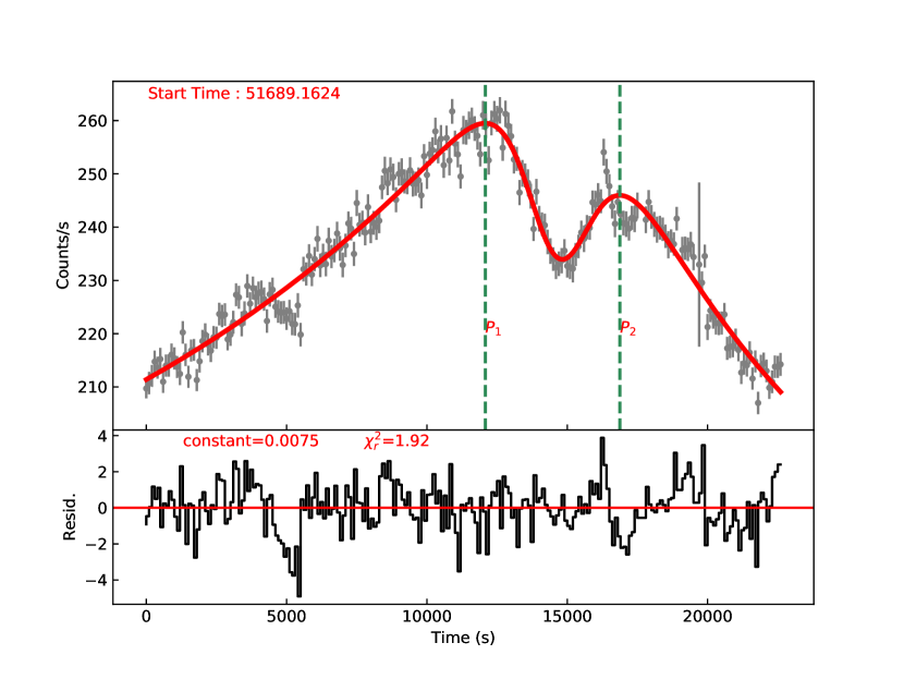
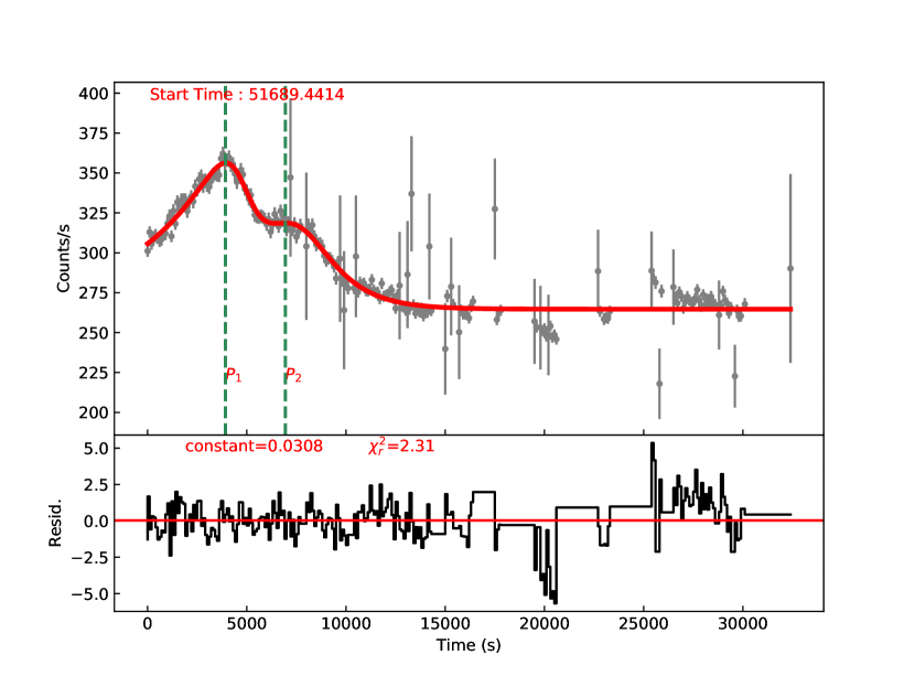
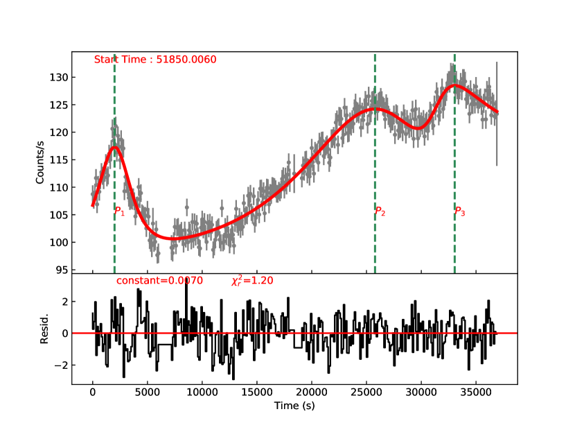
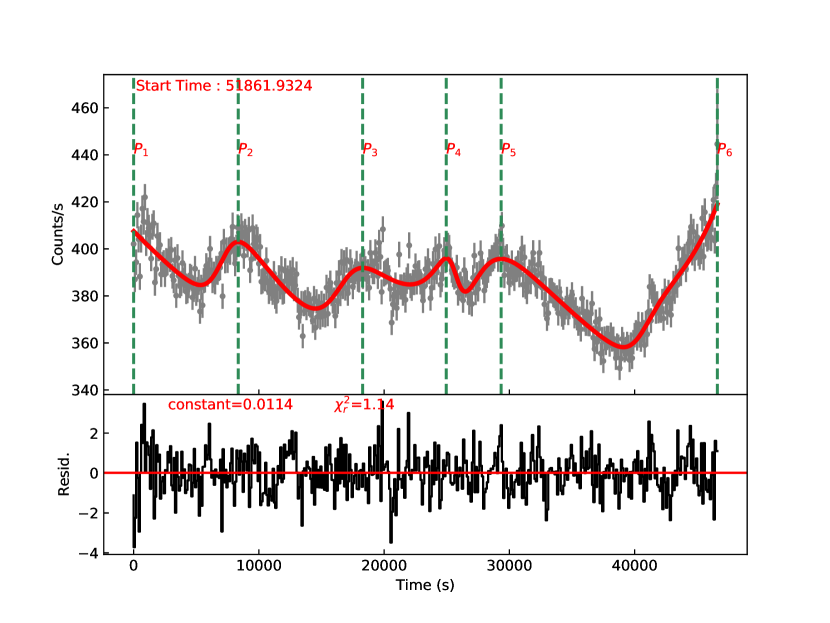
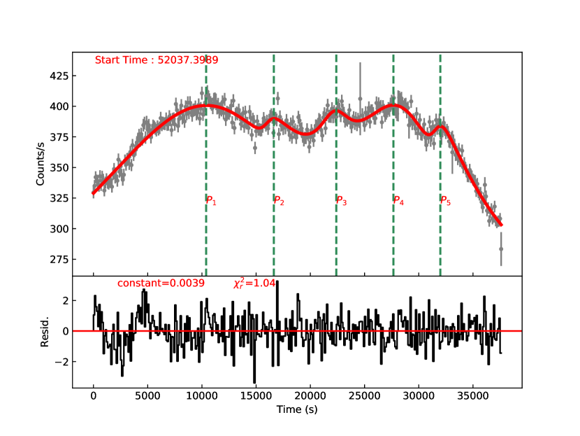
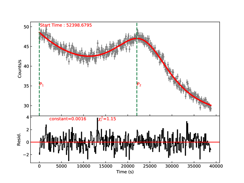
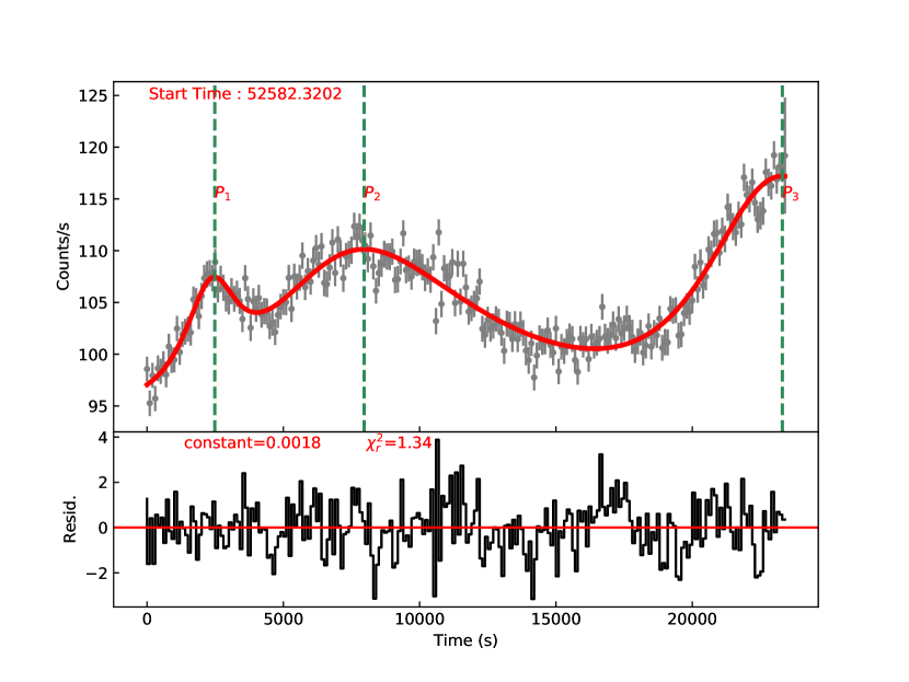
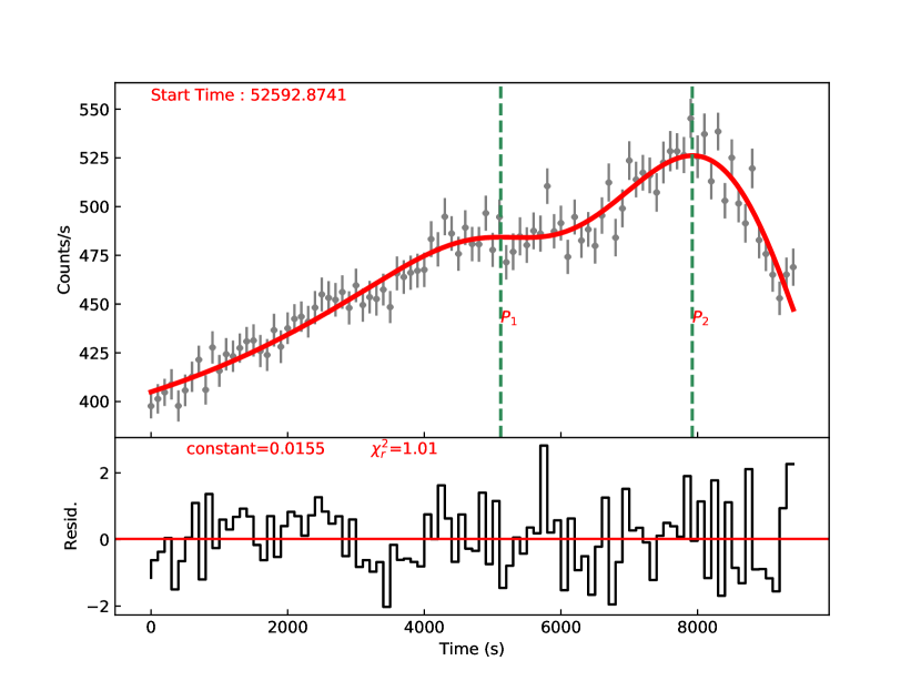
Figure 1: The best-fitting results for light curves. In each panel: the gray points are the observation data; the thick red line is the best-fitting model; the green vertical line indicates the light curves peaking at these time, and every peak is marked by a red word. The distribution of the residuals obtained in each fitting is also showed (the bottom in each panel), which is fitted by a constant (thin red line).

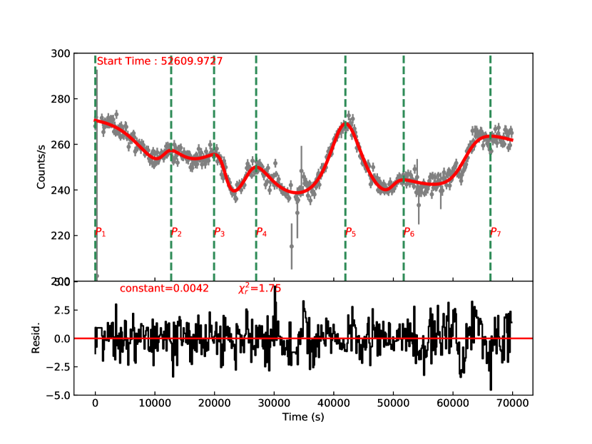
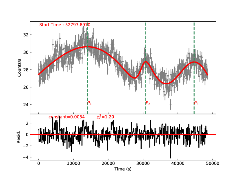
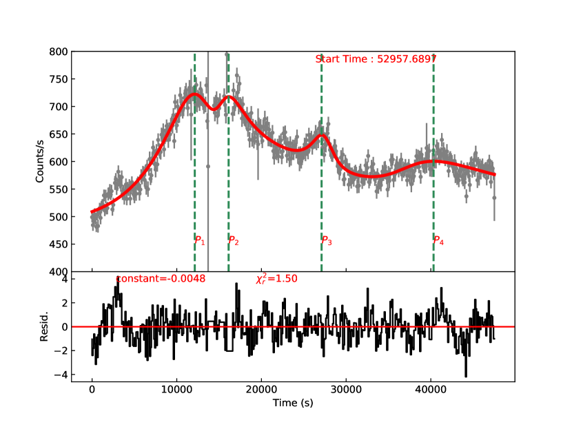
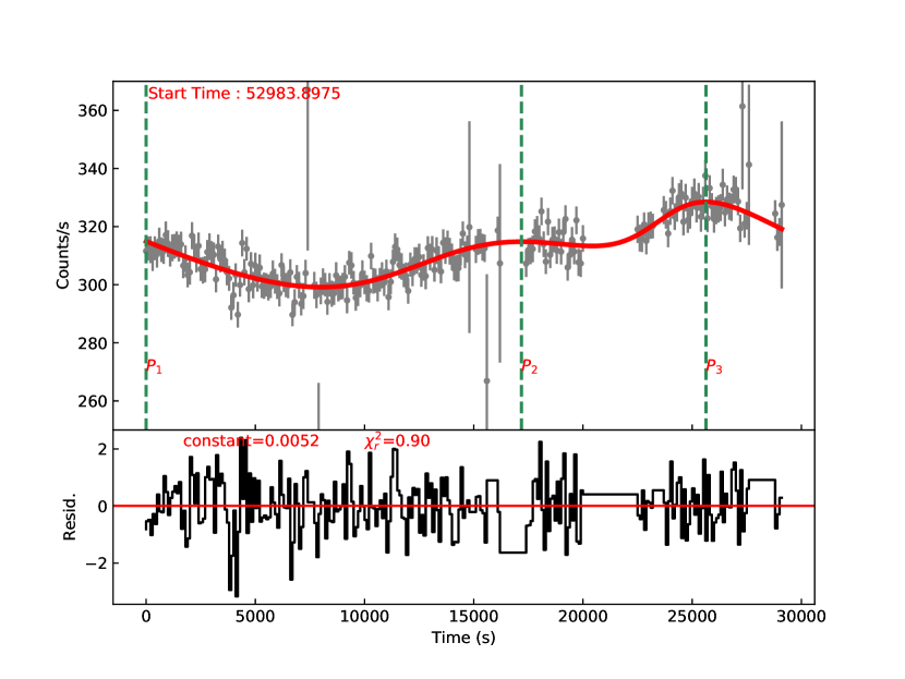
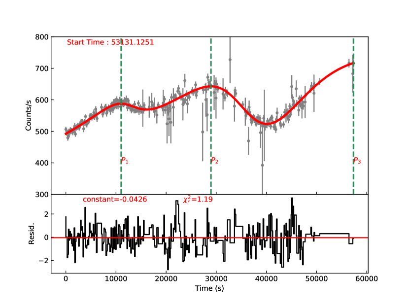
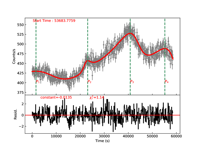
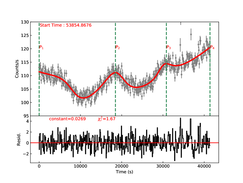
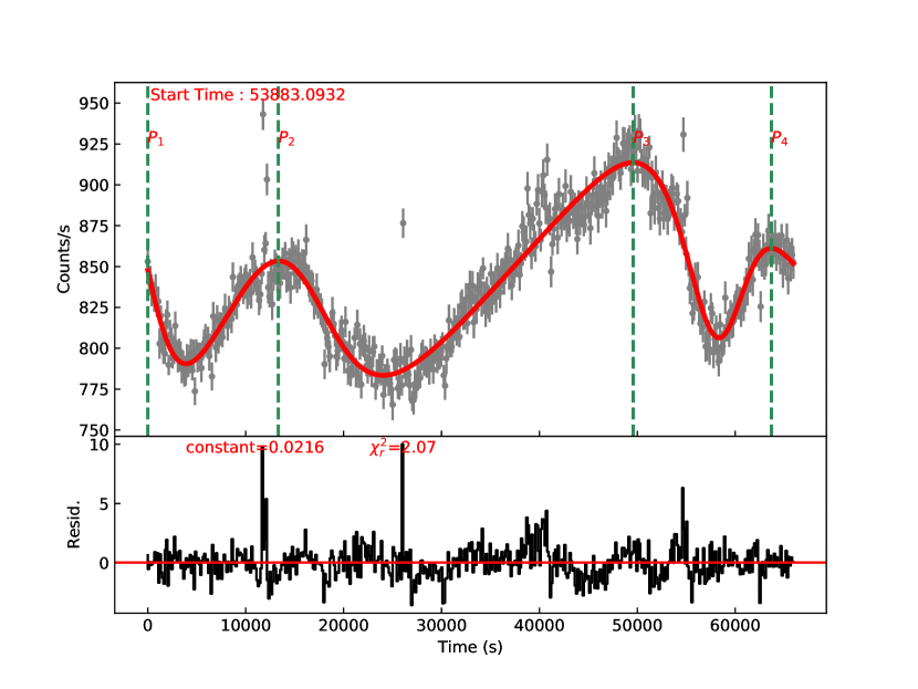
Figure 1: Continued.

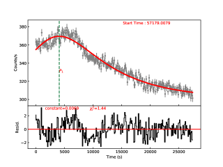
Figure 1: Continued.

Table 3: The results of light-curve fittings. (1) The start time, (2) the observation ID, (3) the observation instrument, (4) the observation filter, (5) the peak number, (6-8) the parameters in equation (1), (9) the flaring time duration, (10) the symmetry parameter $\xi$, (11) the peak flux, in units of $10^{-11}$ ergs/cm²/s, (12) the reduced chi-square of the fitting for each light curve.

StartTime	Obs.ID	Instru.	Filter	Peak NO.	$t_{0}$	$T_{r}$	$T_{d}$	$\rm{T_{fl}}$	$\xi$	$\rm{F_{peak}}$	$\chi^{2}_{r}$
(MJD)					(ks)	(ks)	(ks)	(ks)
51689.1624	0099280101	EPN	Thick	p1	14.0 $\pm$ 0.2	17.0 $\pm$ 4.2	0.8 $\pm$ 0.1	35.5 $\pm$ 5.9	-0.91 $\pm$ 0.32	61.84	2
				p2	15.3 $\pm$ 0.3	0.9 $\pm$ 0.1	8.4 $\pm$ 2.2	18.6 $\pm$ 3.2	0.80 $\pm$ 0.31	58.62
51689.4414	0099280101	EPN	Thick	p1	4.8 $\pm$ 0.1	4.6 $\pm$ 0.8	0.6 $\pm$ 0.2	10.5 $\pm$ 1.2	-0.77 $\pm$ 0.20	86.39	2.41
				p2	7.5 $\pm$ 0.6	2.0 $\pm$ 1.6	1.6 $\pm$ 0.3	7.4 $\pm$ 2.3	-0.11 $\pm$ 0.44	77.27
51850.006	0099280201	EPN	Thick	p1	2.1 $\pm$ 0.3	1.5 $\pm$ 0.2	1.2 $\pm$ 0.2	5.4 $\pm$ 0.4	-0.09 $\pm$ 0.11	25.04	1.25
				p2	26.6 $\pm$ 1.3	6.6 $\pm$ 1.2	4.9 $\pm$ 1.5	22.9 $\pm$ 2.8	-0.15 $\pm$ 0.17	26.52
				p3	31.3 $\pm$ 0.2	0.8 $\pm$ 0.2	3565.1 $\pm$ 316037.0	-	-	27.42
51861.9324	0099280301	EPN	Thick	p2	7.2 $\pm$ 0.4	0.7 $\pm$ 0.2	9.6 $\pm$ 12.3	-	-	99.41	1.22
				p3	16.6 $\pm$ 0.6	1.0 $\pm$ 0.4	13.1 $\pm$ 21.3	-	-	96.68
				p4	25.7 $\pm$ 0.7	5.5 $\pm$ 40.7	0.4 $\pm$ 0.3	-	-	97.68
				p5	26.6 $\pm$ 3.7	-44.0 $\pm$ 197.8	-1.3 $\pm$ 1.2	-	-	97.62
52037.3989	0136540101	EPN	Thin1	p1	12.2 $\pm$ 5.5	11.7 $\pm$ 9.9	7.6 $\pm$ 4.0	38.7 $\pm$ 15.1	-0.21 $\pm$ 0.56	64.11	1.12
				p2	16.0 $\pm$ 0.3	0.4 $\pm$ 0.2	29.2 $\pm$ 256.7	-	-	62.39
				p3	22.2 $\pm$ 0.8	1.2 $\pm$ 0.7	1.3 $\pm$ 1.0	4.9 $\pm$ 1.7	0.04 $\pm$ 0.50	63.42
				p4	27.9 $\pm$ 2.6	3.5 $\pm$ 3.6	5.1 $\pm$ 2.6	-	-	64.15
				p5	31.5 $\pm$ 0.3	0.4 $\pm$ 0.1	31.8 $\pm$ 384.2	-	-	61.39
52582.3202	0136540401	EMOS1	Thin1	p1	2.4 $\pm$ 0.4	0.8 $\pm$ 0.4	0.7 $\pm$ 0.3	3.2 $\pm$ 0.7	-0.06 $\pm$ 0.31	71.97	1.43
				p2	6.7 $\pm$ 0.6	2.3 $\pm$ 0.6	5.2 $\pm$ 1.0	14.8 $\pm$ 1.7	0.39 $\pm$ 0.17	73.76
52592.8741	0136540801	EPN	Thick	p1	5.4 $\pm$ 0.6	71.4 $\pm$ 1667.5	-0.6 $\pm$ 0.5	-	-	143.9	1.12
				p2	9.1 $\pm$ 0.8	3.8 $\pm$ 4.3	1.0 $\pm$ 1.0	-	-	156.4
52609.9727	0136541001	EPN	Medium	p2	11.8 $\pm$ 0.9	0.9 $\pm$ 0.6	4.2 $\pm$ 7.3	-	-	40.5	1.88
				p3	21.7 $\pm$ 0.3	-0.6 $\pm$ 0.1	-9.9 $\pm$ 11.8	-	-	40.22
				p4	26.0 $\pm$ 0.6	1.4 $\pm$ 0.5	3.7 $\pm$ 1.2	10.3 $\pm$ 1.8	0.44 $\pm$ 0.27	39.34
				p5	41.8 $\pm$ 0.2	2.4 $\pm$ 0.2	2.7 $\pm$ 0.3	10.2 $\pm$ 0.5	0.07 $\pm$ 0.07	42.34
				p6	49.9 $\pm$ 0.3	-29.5 $\pm$ 29.8	-0.7 $\pm$ 0.3	-	-	38.46
				p7	62.1 $\pm$ 0.3	1.4 $\pm$ 0.3	45.6 $\pm$ 35.8	94.1 $\pm$ 50.6	0.94 $\pm$ 1.04	41.48
52957.6897	0150498701	EPN	Thin1	p1	13.3 $\pm$ 0.4	4.8 $\pm$ 0.7	1.9 $\pm$ 0.4	13.4 $\pm$ 1.2	-0.44 $\pm$ 0.14	115.9	1.56
				p2	15.2 $\pm$ 0.2	0.7 $\pm$ 0.1	19.4 $\pm$ 4.5	40.2 $\pm$ 6.4	0.93 $\pm$ 0.31	115.2
				p3	27.4 $\pm$ 0.5	1.3 $\pm$ 0.4	0.9 $\pm$ 0.3	4.5 $\pm$ 0.8	-0.19 $\pm$ 0.25	104
				p4	37.2 $\pm$ 0.9	-25.4 $\pm$ 16.9	-2.0 $\pm$ 0.8	54.8 $\pm$ 23.9	0.85 $\pm$ 0.81	96.35
52398.6795	0153950601	EMOS1	Thin1	p2	24.1 $\pm$ 0.5	7.1 $\pm$ 0.8	4.8 $\pm$ 0.3	23.8 $\pm$ 1.2	-0.20 $\pm$ 0.07	26.06	1.17
52797.897	0158970701	EMOS1	Thick	p1	26.1 $\pm$ 18.3	44.2 $\pm$ 67.7	12.3 $\pm$ 4.9	-	-	25.24	1.23
				p2	29.8 $\pm$ 0.5	0.9 $\pm$ 0.2	5.5 $\pm$ 3.6	12.9 $\pm$ 5.0	0.72 $\pm$ 0.68	23.83
				p3	42.7 $\pm$ 3.4	4.5 $\pm$ 2.5	16.7 $\pm$ 28.5	-	-	23.8
53131.1251	0158971201	EPN	Medium	p1	12.6 $\pm$ 1.4	13.9 $\pm$ 21.1	2.1 $\pm$ 0.4	-	-	104.8	1.26
				p2	35.1 $\pm$ 5.9	51.9 $\pm$ 588.8	3.5 $\pm$ 0.4	-	-	114.6
53683.7759	0158971301	EPN	Thick	p1	7.8 $\pm$ 5.6	96.6 $\pm$ 823.1	3.5 $\pm$ 2.9	-	-	100.5	1.18
				p2	22.2 $\pm$ 0.6	0.8 $\pm$ 0.4	2.2 $\pm$ 0.9	6.2 $\pm$ 1.4	0.46 $\pm$ 0.36	107
				p3	43.7 $\pm$ 0.4	19.7 $\pm$ 8.0	1.7 $\pm$ 0.3	42.9 $\pm$ 11.3	-0.84 $\pm$ 0.49	123.5
				p4	60.0 $\pm$ 1.4	30.2 $\pm$ 27.5	1.8 $\pm$ 0.8	63.9 $\pm$ 38.9	-0.89 $\pm$ 1.15	114.3
52983.8975	0162960101	EPN	Medium	p2	12.8 $\pm$ 7.0	2.7 $\pm$ 3.9	76.6 $\pm$ 1914.1	-	-	53.65	0.95
				p3	23.7 $\pm$ 3.2	1.2 $\pm$ 1.4	21.5 $\pm$ 282.3	-	-	55.98
53854.8676	0302180101	EMOS2	Thin1	p2	19.3 $\pm$ 0.6	4.3 $\pm$ 1.8	1.5 $\pm$ 0.3	11.7 $\pm$ 2.6	-0.48 $\pm$ 0.36	84.02	1.76
				p3	29.9 $\pm$ 0.7	1.1 $\pm$ 0.5	2.0 $\pm$ 0.9	6.3 $\pm$ 1.4	0.29 $\pm$ 0.33	86.52
53883.0932	0411080301	EPN	Medium	p2	16.8 $\pm$ 0.7	24.1 $\pm$ 10.8	3.2 $\pm$ 0.4	54.6 $\pm$ 15.2	-0.77 $\pm$ 0.50	184.5	2.15
				p3	59.3 $\pm$ 1.5	4843.5 $\pm$325805.3	2.2 $\pm$ 0.7	-	-	197.5
				p4	59.3 $\pm$ 2.3	2.2 $\pm$ 0.4	9298.6 $\pm$ 597976.9	-	-	186.2
57179.0079	0658801301	EPN	Thick	p1	2.1 $\pm$ 0.8	4.4 $\pm$ 0.7	8.5 $\pm$ 1.0	25.7 $\pm$ 1.7	0.32 $\pm$ 0.10	82.69	1.46

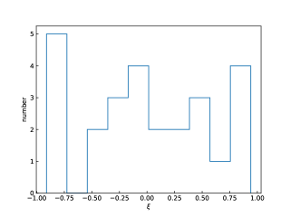
Figure 4: Distribution of flare symmetry parameter $\xi$.

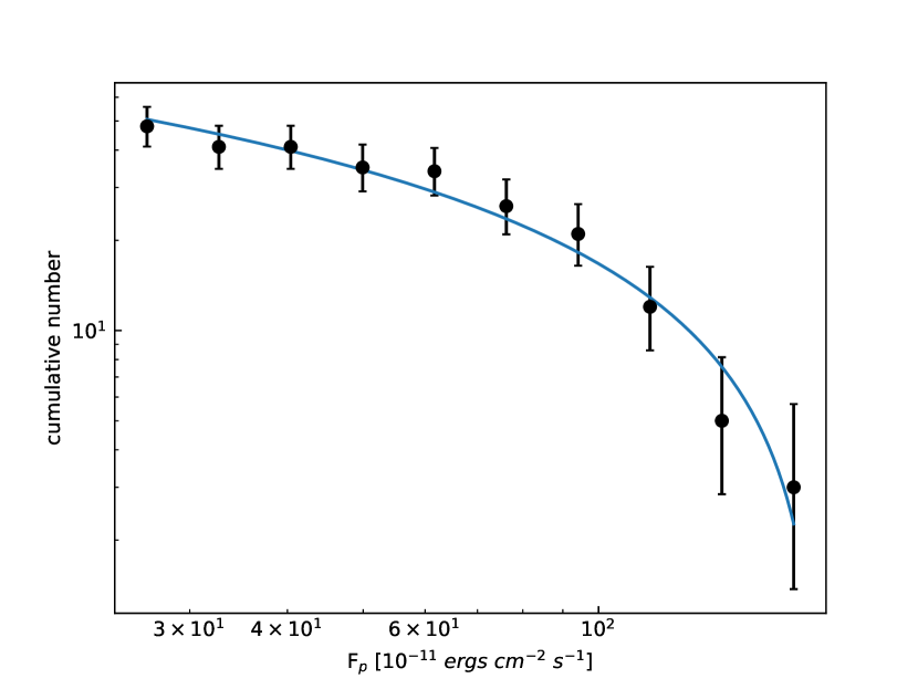
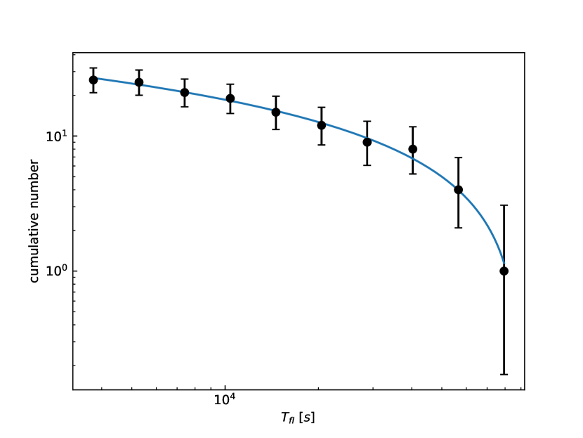
Figure 5: Cumulative distributions of peak flux (left) and flaring time duration (right). The solid lines are the best-fitting results to the distributions with the equation (4).

4 Conclusions and discussion

We analyzed 50 XMM-Newton X-ray observations for Mrk 421, and constructed the X-ray light curves. The basic information, such as $F_{\rm var}$ and NPSD can be found in Appendix. We fitted the 17 light curves which have one complete flare-profile at least, in order to determine the flare rise and decay times as well as peak fluxes (see Fig. 1). We obtained these parameters for 48 flares. Among them, 26 flares have well constrained parameters (see Table 3). The flaring time duration is evaluated by using the flare rise and decay times. It is found that both the peak flux and flaring time duration distributions follow a power-law form with the same index of $\alpha_{\rm F}=\alpha_{\rm T}\approx 1$.

It has been argued that the behavior that event parameters obey a power-law distribution is a characteristic of SOC system (e.g., Aschwanden, 2012). The SOC model has been used to explain astrophysical X-ray flares, such as GRB X-ray flares (Wang & Dai, 2013; Yi et al., 2016, 2017) and super massive black hole (SMBH) X-ray flares (Wang et al., 2015; Li et al., 2015). They found that the statistical properties of the GRB and SMBH X-ray flares can be explained by a fractal-diffusive SOC model, but with different spatial dimensions $S$ ($S=1$ for GRB X-ray flares and $S=3$ for SMBH X-ray flares). However, Yuan et al. (2018) argued that a simple SOC model failed to explain the X-ray flares in SMBH Sgr A^∗.

The SOC model expects the index of peak flux distribution $\alpha_{\rm F}=1+(S-1)/D_{S}$ ($D_{S}$ is the fractal Hausdorff dimension, spanning from 1 to $S$), and the index of flaring time duration distribution $\alpha_{\rm T}=1+(S-1)\beta/S$ where $\beta$ is a diffusion parameter (e.g., Aschwanden, 2012). The statistical results of Mrk 421 X-ray flares are consistent with the expectation of a SOC mode with $S=1$. This indicates that the X-ray flares of Mrk 421 are possibly driven by magnetic reconnection. Our results support the finding that magnetic reconnection is a promising process for energy dissipation in blazar jet (Sironi et al., 2015).

The $S$ of Mrk 421 is similar to that of GRB X-ray flares, but different from that of X-ray flares in M87 and Sgr A^∗ (i.e., the SMBH X-ray flares). M87 is a radio galaxy. It is thought that the main difference between radio galaxy and blazar is the angle of jet direction with respect to the line-of-sight. We notice that the flaring time duration for M87 in Wang et al. (2015) spans from 0.2 years to several years. Such a long timescale indicates that the X-ray emissions come from a large region which locates relatively far away from the central SMBH. On the other hand, the rapid X-ray emission from blazar is believed to come from a region locating at sub-pc scale. It is possible that the results of M87 and Mrk 421 reveal the situations about magnetic field in different regions along the jet in radio-loud AGN. However, note that the uncertainties on the results of M87 are very large (Wang et al., 2015).

Sub-hour variabilities are presented in our analysis. Flares with $t_{\rm var}\sim t_{\rm d}\sim 1000\$s frequently appear. Such rapid flare indicates that the magnetic field in emission region is $B^{\prime}\geq 2.1\delta_{\rm D}^{-1/3}$ G. This magnetic field is much higher than the value of $B^{\prime}<0.1\$G that derived in SSC modeling of SED (e.g., Yan et al., 2013; Zhu et al., 2016). Taking advantage of the radio core-shift-effect obtained in Very Long Baseline Array (VLBA) observations, Zamaninasab et al. (2014) derived the magnetic field strength $B^{\prime}_{\rm 1pc}$ at one pc along the jet for tens blazars, and they found $B^{\prime}_{\rm 1pc}$ spanning from 0.2 G to 2 G. This is consistent with the magnetic field strength expected by a magnetically powered jet (e.g., O’Sullivan & Gabuzda, 2009). If Mrk 421 is not a outlier, the magnetic field of $B^{\prime}\geq 2.1\delta_{\rm D}^{-1/3}$ G is also likely consistent with the prediction of a magnetically powered jet. For a magnetically powered jet, magnetic reconnection is a natural candidate for energy dissipation in blazar jet (e.g., Sironi et al., 2015).

As a last remark, we note that Zubovas et al. (2012) proposed a model of tidal disruption of asteroids by the SMBH for the origin of Sgr A^∗ X-ray flares. This model probably also can explain the power-law distributions of the parameters of Sgr A^∗ X-ray flares (Zubovas et al., 2012). However, this scenario will not happen in blazar (e.g., Komossa, 2015), due to the SMBH with the mass of $\gtrsim 10^{8}M_{\odot}$ in blazar, where $M_{\odot}$ is the solar mass. As far as we know, the SOC model is the only model for explaining the power-law distributions of the parameters of blazar flares.

Appendix A Fifty XMM-Newton X-ray light curves of Mrk 421

In Fig. 4, we show all fifty XMM-Newton X-ray light curves obtained in our analysis. To characterize the variability amplitude for each light curve, we use the fraction root mean square (rms) variability amplitude (Vaughan et al., 2003),

$$F_{\rm{var}}=\sqrt{\frac{S^{2}-\overline{\sigma^{2}_{\rm{err}}}}{\overline{x}^{2}}}\ ,$$ (A1)

where $S^{2}$ is the variance of the light curve; $\overline{\sigma^{2}_{\rm{err}}}$ is the mean square error of the light curve, and $\overline{x}^{2}$ is the arithmetic mean of the data. The error of the $F_{\rm{var}}$ is calculated using the Equation B2 in (Vaughan et al., 2003). The results of the calculations are listed in Table 4.

The general timing analysis technique for characterizing the light curve is power spectrum density (PSD). However, because of the orbital effects of satellites and some CCD background problems, the X-ray light curves extracted from the clear events are usually uneven. To getting correct PSD calculations, we adopt the method called normalized power spectrum density (NPSD; e.g., Hayashida et al., 1998; Kataoka et al., 2001). The calculated frequency range is from 1/T to 1/(2$\times$bin) where T is the timing coverage and “bin” is the bin size of the light curve. If the light curve contains $n$ time gaps larger than twice the data bin size, each gap is considered as a break so that the light curve is separated into $n+1$ segments. Then the total power of the light curve is the average of the powers of these segments. Note that we do not subtract the white noise power in each calculation.

We then fit the NPSDs using a power-law form function,

$$P=af^{-\alpha}+b\,$$ (A2)

where $P$ is the NPSD power, $f$ the frequency, $\alpha$ the power-law index, $b$ the white noise power, and $a$ a constant. The NPSD for each light curve and its best-fitting result is shown in Figure 4. The best-fitting values of $\alpha$ and $b$ are listed in Table 4. The distribution of $\alpha$ is shown in Fig. 5. The poorly constrained $\alpha$ are excluded in Fig. 5. One can see that $\alpha$ spans between 1 and 3, and most of them cluster around 2.

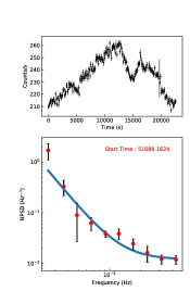
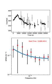
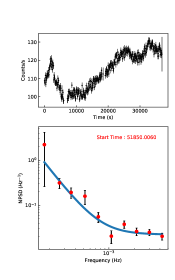
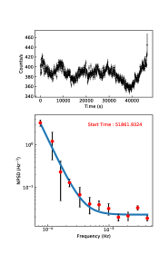
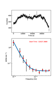
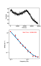
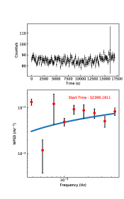
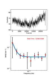
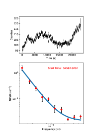
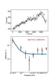
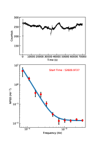
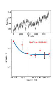
Figure 4: Fifty light curves and the corresponding NPSD. The upper panel is the light curve, and the lower panel is the NPSD. The red points are the calculated NPSD, and the steel blue line is the best fitting. The start time of each light curve is marked using the MJD in the lower panel.

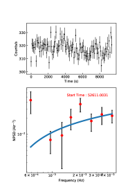
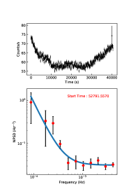
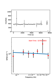
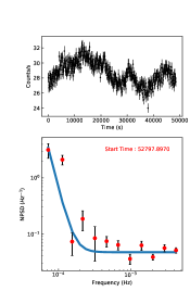
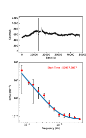
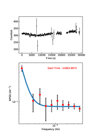
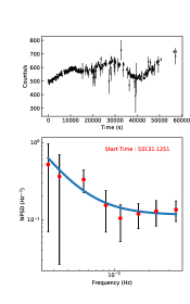
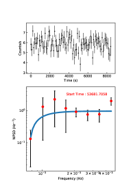
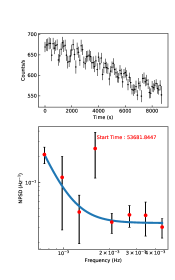
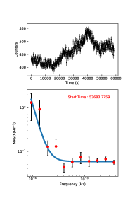
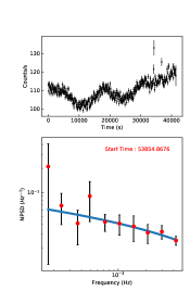
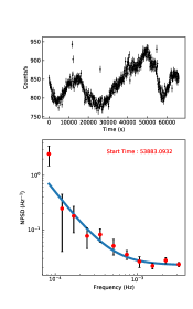
Figure 4: Continued.

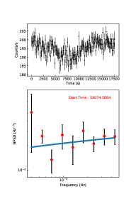
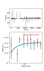
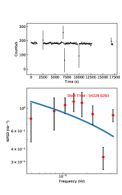
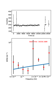
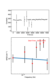
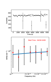
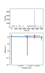
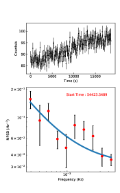
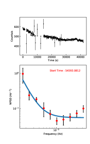
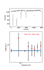
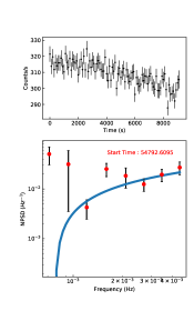
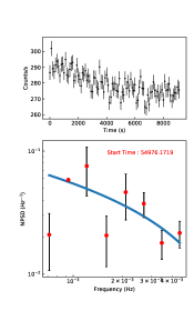
Figure 4: Continued.

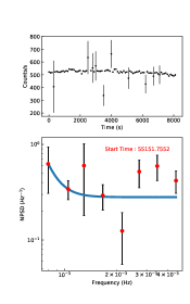
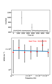
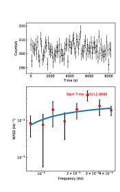
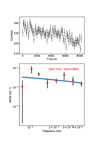
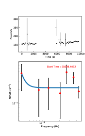
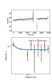
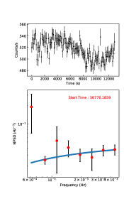
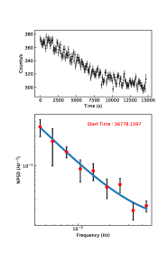
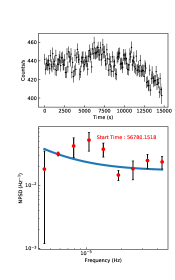
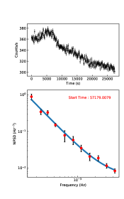
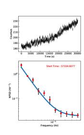
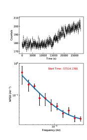
Figure 4: Continued.

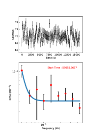
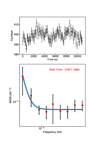
Figure 4: Continued.

Table 4: The NPSD best-fitting results and $F_{\rm{var}}$. (1) The start time, (2) the observation ID, (3) the power-law index, (4) the white noise power, (5) the reduced chi-square of the NPSD fitting, (6)the fraction variability amplitude of the light curve.

StartTime	Obs.ID	$\alpha$	$b$	$\chi^{2}_{r}$	$F_{\rm{var}}$
(MJD)
51689.1624	0099280101	2.52 $\pm$ 0.42	0.0119 $\pm$ 0.0020	1.136	0.0609 $\pm$ 0.0004
51689.4414	0099280101	1.34 $\pm$ 1.13	0.0657 $\pm$ 0.0231	0.427	0.1032 $\pm$ 0.0463
51850.006	0099280201	2.42 $\pm$ 0.49	0.0224 $\pm$ 0.0031	1.381	0.0814 $\pm$ 0.0002
51861.9324	0099280301	3.04 $\pm$ 0.30	0.0225 $\pm$ 0.0021	1.564	0.0320 $\pm$ 0.0063
52037.3989	0136540101	2.68 $\pm$ 0.25	0.0325 $\pm$ 0.0017	0.441	0.0621 $\pm$ 0.0023
52582.0308	0136540301	4.28 $\pm$ -	0.0355 $\pm$ -	0.552	0.0273 $\pm$ 0.0031
52582.3202	0136540401	2.36 $\pm$ 0.30	0.0134 $\pm$ 0.0034	1.976	0.0433 $\pm$ 0.0003
52592.8741	0136540801	5.32 $\pm$ -	0.0232 $\pm$ -	3.567	0.0761 $\pm$ 0.0251
52609.9727	0136541001	3.16 $\pm$ 0.23	0.0142 $\pm$ 0.0011	0.998	0.0347 $\pm$ 0.0055
52610.8351	0136541101	5.07 $\pm$ -	0.0486 $\pm$ -	1.452	0.0410 $\pm$ 0.0523
52611.0031	0136541201	0.06 $\pm$ 2.64	0.1643 $\pm$ 6.3031	1.712	0.0080 $\pm$ 0.3564
52957.6897	0150498701	2.11 $\pm$ 0.13	0.0677 $\pm$ 0.0058	0.621	0.0725 $\pm$ 0.5272
52398.6795	0153950601	1.91 $\pm$ 0.06	0.0243 $\pm$ 0.0046	0.978	0.1242 $\pm$ 0.00002
52399.1911	0153950701	0.01 $\pm$ 2.90	1.5690 $\pm$ 357.4908	7.162	nan $\pm$ nan
53681.8447	0153951201	4.24 $\pm$ -	0.0336 $\pm$ 0.0041	0.662	0.0578 $\pm$ 0.1419
53681.7058	0153951301	3.63 $\pm$ 12.24	0.9653 $\pm$ 0.2500	1.133	0.0389 $\pm$ 0.0164
52791.557	0158970101	2.37 $\pm$ 0.36	0.0314 $\pm$ 0.0024	0.841	0.0635 $\pm$ 0.0001
52792.0603	0158970201	0.01 $\pm$ 8.71	-17.7281 $\pm$ 29382.3219	0.815	nan $\pm$ nan
52797.897	0158970701	5.22 $\pm$ -	0.0468 $\pm$ -	4.091	0.0455 $\pm$ 0.0001
53131.1251	0158971201	2.02 $\pm$ 0.82	0.1148 $\pm$ 0.0204	0.336	0.0690 $\pm$ 0.2558
53683.7759	0158971301	4.42 $\pm$ -	0.0584 $\pm$ -	0.907	0.0786 $\pm$ 0.0082
52983.8975	0162960101	3.80 $\pm$ -	0.0775 $\pm$ 0.0039	0.402	0.0325 $\pm$ 0.0928
53854.8676	0302180101	0.05 $\pm$ 0.54	-0.1917 $\pm$ 2.5311	0.312	0.0454 $\pm$ 0.0002
53883.0932	0411080301	1.97 $\pm$ 0.43	0.0224 $\pm$ 0.0021	1.018	0.0468 $\pm$ 0.0037
54074.5064	0411080701	0.00 $\pm$ 4.51	0.6957 $\pm$ 826.7401	1.183	0.0147 $\pm$ 0.0307
54230.1689	0411081301	0.02 $\pm$ 6.58	2.3858 $\pm$ 768.9216	2.813	nan $\pm$ nan
54230.4143	0411081401	0.01 $\pm$ 13.06	-7.7254 $\pm$ 10649.9636	2.761	nan $\pm$ nan
54230.5439	0411081501	0.12 $\pm$ 5.36	1.8319 $\pm$ 42.4040	0.126	0.0564 $\pm$ 4.4417
54230.6735	0411081601	0.03 $\pm$ 12.65	-518.7431 $\pm$ 252525.5077	0.292	nan $\pm$ nan
54423.5489	0411081901	1.06 $\pm$ 0.58	0.0311 $\pm$ 0.0127	1.297	0.0330 $\pm$ 0.0104
54617.1091	0411082701	0.77 $\pm$ 2115.67	0.4956 $\pm$ 0.6055	0.461	0.0749 $\pm$ 12.2353
55151.7552	0411083201	6.54 $\pm$ -	0.2805 $\pm$ -	2.476	nan $\pm$ nan
54593.0812	0502030101	2.50 $\pm$ 0.92	0.0552 $\pm$ 0.0101	1.744	0.0682 $\pm$ 0.0254
54228.6283	0510610101	0.02 $\pm$ 2.42	-14.6276 $\pm$ 2161.6860	5.009	0.0434 $\pm$ 2.7936
54228.3529	0510610201	1.39 $\pm$ 2.79	0.4236 $\pm$ 0.1005	1.290	nan $\pm$ nan
54792.6095	0560980101	0.01 $\pm$ 3.13	1.7160 $\pm$ 722.0796	2.956	0.0175 $\pm$ 0.0967
54976.1719	0560983301	0.12 $\pm$ 1.95	-0.1620 $\pm$ 3.0696	5.601	0.0216 $\pm$ 0.0635
55319.3278	0656380101	0.01 $\pm$ 22.24	-2.5869 $\pm$ 9925.8947	0.324	0.1127 $\pm$ 4.9136
55512.8889	0656380801	0.60 $\pm$ 2.22	0.0296 $\pm$ 0.0502	1.126	nan $\pm$ nan
55514.8844	0656381301	0.01 $\pm$ 3.52	-1.0512 $\pm$ 399.0310	3.349	0.0174 $\pm$ 0.0731
55698.4452	0658800101	6.71 $\pm$ -	0.2205 $\pm$ -	1.088	nan $\pm$ nan
55894.0036	0658800801	4.32 $\pm$ -	0.0790 $\pm$ -	0.533	0.0123 $\pm$ 0.2107
57179.0079	0658801301	1.66 $\pm$ 0.12	0.0056 $\pm$ 0.0016	0.890	0.0654 $\pm$ 0.0007
57334.6077	0658801801	2.23 $\pm$ 0.18	0.0197 $\pm$ 0.0032	1.075	0.0677 $\pm$ 0.0006
57514.17	0658802301	1.42 $\pm$ 0.20	0.0144 $\pm$ 0.0032	0.472	0.0444 $\pm$ 0.0016
56776.1859	0670920301	0.36 $\pm$ 2.69	0.0513 $\pm$ 0.1450	0.693	0.0241 $\pm$ 0.2352
56778.1597	0670920401	1.65 $\pm$ 0.32	0.0123 $\pm$ 0.0074	0.593	0.0676 $\pm$ 0.0051
56780.1518	0670920501	1.41 $\pm$ 3.22	0.0170 $\pm$ 0.0113	2.390	0.0207 $\pm$ 0.0597
57695.5677	0791780101	6.51 $\pm$ -	0.0307 $\pm$ -	0.981	0.0071 $\pm$ 0.0336
57877.186	0791780601	6.92 $\pm$ -	0.0068 $\pm$ -	0.342	0.0057 $\pm$ 0.2461

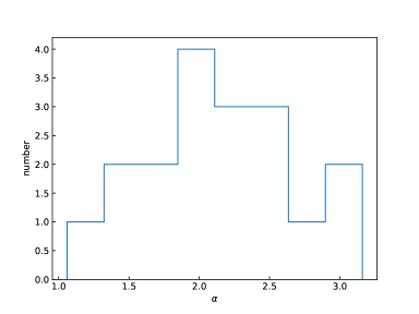
Figure 5: Distribution of the index of NPSD $\alpha$.

References

- Abdo et al. (2010) Abdo, A. A., Ackermann, M., Ajello, M., et al. 2010, ApJ, 722, 520
- Ackermann et al. (2016) Ackermann, M., Anantua, R., Asano, K., et al. 2016, ApJ, 824, L20
- Aharonian (2000) Aharonian F. A., 2000, NewA, 5, 337
- Aharonian et al. (2007) Aharonian, F., Akhperjanian, A. G., Bazer-Bachi, A. R., et al. 2007, ApJL, 664, L71
- Aharonian et al. (2017) Aharonian, F. A., Barkov, M. V., Khangulyan, D., 2017, ApJ, 841, 61
- Arnaud (1996) Arnaud, K. A., 1996, ASPC, 101, 17
- Aschwanden (2011) Aschwanden, M. J., 2011, Solar Physics, 274, 99
- Aschwanden (2012) Aschwanden, M. J., 2012, A&A, 539, A2
- Barkov et al. (2012) Barkov, M. V., Aharonian, F. A., Bogovalov, S. V., Kelner, S. R., & Khangulyan, D. 2012, ApJ, 749, 119
- Böttcher et al. (2003) Böttcher M., Marscher A. P., Ravasio M. et al., 2003, ApJ, 596, 847
- Böttcher et al. (2009) Böttcher M., Reimer A., Marscher A. P., 2009, ApJ, 703, 1168
- Cerruti et al. (2015) Cerruti M., Zech A., Boisson C., Inoue S. 2015, MNRAS, 448, 910
- Chen et al. (2016) Chen, X. H., Pohl, M., Böttcher M., Gao, S., 2016, MNRAS, 458, 3260
- Cui (2004) Cui, W., 2004, ApJ, 605, 662
- Dai et al. (2015) Dai, B. Z., Zeng, W., Jiang, Z. J., et al. 2015, ApJS, 218, 18
- Dermer & Schlickeiser (1993) Dermer C. D., Schlickeiser R., 1993, ApJ, 416, 458
- Li et al. (2015) Li Y. P. et al., 2015, ApJ, 810, 19
- Lu & Hamilton (1991) Lu, E. T., & Hamilton, R. J., 1991, ApJ, 380, L89
- Fossati et al. (2008) Fossati, G. et al. 2008, ApJ , 677, 906
- Gehrels (1986) Gehrels, N. 1986, ApJ, 303, 336
- Giannios et al. (2009) Giannios, D., Uzdensky, D. A., & Begelman, M. C. 2009, MNRAS, 395, L29
- Harris et al. (2003) Harris, D., Biretta, J., Junor, W. et al., 2003, ApJ, 586, L41
- Hayashida et al. (1998) Hayashida, K., Miyamoto, S., Kitamoto, S., Negoro, H., & Inoue, H. 1998, ApJ, 500, 642
- Kalberla et al. (2005) Kalberla, P. M. W., Burton, W. B., Hartmann, D., et al. 2005, A&A, 440, 775
- Kapanadze et al. (2016) Kapanadze et al., 2016, ApJ, 831, 102
- Kapanadze et al. (2018) Kapanadze et al., 2018, ApJ, 854, 66
- Kataoka et al. (2001) Kataoka, J., Takahashi, T., Edwards, P. G., et al. 2001, American Institute of Physics Conference Series, 558, 660
- Komossa (2015) Komossa, S., 2015, JHEAp, 7, 148
- Maraschi et al. (1992) Maraschi L., Ghisellini G., Celotti A., 1992, ApJL, 397, L5
- Mannheim & Biermann (1992) Mannheim, K., & Biermann, P. L. 1992, A&A, 253, L21
- Mukai (1993) Mukai, K., 1993, Legacy 3, 21
- Mücke & Protheroe (2001) Mücke A., Protheroe R. J., 2001, APh, 15, 121
- Mücke et al. (2003) Mücke A., Protheroe R. J., Engel R., Rachen J. P., Stanev T., 2003, APh, 18, 593
- Neronov & Aharonian (2007) Neronov, A., & Aharonian, F. A. 2007, ApJ, 671, 85
- O’Sullivan & Gabuzda (2009) O’Sullivan, S. P., & Gabuzda, D. C. 2009, MNRAS, 400, 26
- Padovani & Giommi (1995) Padovani, P., & Giommi, P. 1995, ApJ, 444, 567
- Paliya et al. (2015) Paliya, V. S., Böttcher, M., Diltz, C., Stalin, C. S., Sahayanathan, S., Ravikumar, C. D., 2015, ApJ, 811, 143
- Sikora et al. (1994) Sikora M., Begelman M. C., Rees M. J., 1994, ApJ, 421, 153
- Sironi et al. (2015) Sironi, L., Petropolou, M., Giannios, D., 2015, MNRAS, 450, 183
- Tavecchio et al. (1998) Tavecchio F., Maraschi L., Ghisellini G., 1998, ApJ, 509, 608
- Vaughan et al. (2003) Vaughan, S., Edelson, R., Warwick, R. S., & Uttley, P. 2003, MNRAS, 345, 1271
- Wang & Dai (2013) Wang, F. Y., & Dai, Z. G. 2013, NatPh, 9, 465
- Wang et al. (2015) Wang, F. Y., Dai, Z. G., Yi, S. X., & Xi, S. Q. 2015, ApJS, 216, 8
- Yan et al. (2013) Yan D. H., Zhang L., Yuan Q., Fan Z. H., Zeng H. D., 2013, ApJ, 765, 122
- Yan & Zhang (2015) Yan D. H., Zhang L., 2015, MNRAS, 447, 2810
- Yan et al. (2018) Yan D. H., Wu, Q. W., Fan, X. L., Wang, J. C., Zhang, L. 2018, ApJ, 859, 168
- Yi et al. (2016) Yi, S. X., Xi, S. Q., Yu, H. et al., 2016, ApJS, 224, 20
- Yi et al. (2017) Yi, S. X., Yu, H., Wang, F.Y., Dai, Z. G., et al., 2016, ApJS, 224, 20
- Yuan et al. (2018) Yuan, Q. Wang, Q. D, Liu, S. M., Wu, K., 2018, MNRAS, 473, 306
- Zamaninasab et al. (2014) Zamaninasab, M., Clausen-Brown, E., Savolainen, T., & Tchekhovskoy, A. 2014, Nature, 510, 126
- Zhu et al. (2018) Zhu, S. F., Xue, Y. Q., Brandt, W. N., Cui, W., Wang, Y. J., 2018, ApJ, 853, 34
- Zhu et al. (2016) Zhu Q. Q., Yan D. H., Zhang P. F., et al., 2016, MNRAS, 463, 4481
- Zubovas et al. (2012) Zubovas, K., Nayakshin, S., Markoff, S., 2012, MNRAS, 421, 1315