Run and tumble particle under resetting: a renewal approach

Abstract

We consider a particle undergoing run and tumble dynamics, in which its velocity stochastically reverses, in one dimension. We study the addition of a Poissonian resetting process occurring with rate $r$. At a reset event the particle’s position is returned to the resetting site $X_{r}$ and the particle’s velocity is reversed with probability $\eta$. The case $\eta=1/2$ corresponds to position resetting and velocity randomization whereas $\eta=0$ corresponds to position-only resetting. We show that, beginning from symmetric initial conditions, the stationary state does not depend on $\eta$ i.e. it is independent of the velocity resetting protocol. However, in the presence of an absorbing boundary at the origin, the survival probability and mean time to absorption do depend on the velocity resetting protocol. Using a renewal equation approach, we show that the mean time to absorption is always less for velocity randomization than for position-only resetting.

Keywords: run and tumble dynamics, persistent random walkers, diffusion, stochastic resetting

1 Introduction

Stochastic processes with correlated noise have a long history in physics beginning with the Ornstein Uhlenbeck process which generates a finite correlation time for Brownian motion [1, 2]. More recently, active matter has been described by stochastic processes with correlated noise such as the run and tumble dynamics used to model bacterial motion. Run and tumble dynamics is, in turn, the continuum limit of persistent random walkers [3, 4] commonly used to model animal movement [5] and search processes [6]. Also the bidirectional motion of cellular cargoes is, in general, a correlated random walk [7].

A particle under run and tumble dynamics, in one dimension, obeys a Langevin equation of the form

$$\frac{{\rm d}x}{{\rm d}t}=v_{0}\sigma(t)$$ (1)

Here $\sigma$ is a stochastic process which switches between two states $\sigma=\pm 1$ with rate $\gamma$; non-Poissonian switching has been considered in [8]. Thus a run and tumble process is sometimes referred to as ‘telegraphic noise’ to describe the evolution of $\sigma$ [9]. The equation for the time evolution of the probability distribution corresponding to (1) turns out to be the Telegrapher’s equation (see e.g. [3]). This equation interpolates between the wave equation and the diffusion equation, i.e., when $\gamma\to 0$ we have ballistic motion and when $\gamma,v_{0}\to\infty$ (see section 3.1 equation (29) for the precise limit) we have diffusive motion.

Run and tumble dynamics have revealed a number of interesting nonequilibrium properties such as clustering at boundaries [10, 11], novel stationary states [12, 13] and first-passage properties [14, 15]. In this paper we investigate the effect of resetting [16] on run and tumble dynamics. Resetting is the procedure of restarting a stochastic process from a given initial condition [17]. It has been shown that resetting profoundly changes the properties of diffusion, a fundamental dynamical process [16].

Our aim in this work is twofold. First run and tumble particle dynamics allows us to investigate how the effect of resetting on a process which interpolates between diffusive and ballistic motion, thus extending previous results which have focussed on diffusion. Second, a stochastic process of the form (1) open up a whole new set of possibilities for resetting, as the velocity variable $\sigma$ as well as the position $x$ may be reset. Thus the resetting occurs in the phase space of the particle rather than just the position space as has usually been considered. (We note that orientation resets have been considered in continuous time random walks with drifts [18].) We focus on the case where the position is reset to a fixed resetting point $X_{r}$ and simultaneously the velocity undergoes a resetting protocol. Initially, we consider velocity randomization in which the velocity is reversed with probability $1/2$. Later we generalise this to the protocol where the velocity is reversed with probability $\eta$ which allows interpolation to the case of position-only resetting where $\eta=0$.

Let us now summarise recent results on resetting of stochastic processes. In the case of position resetting, the resetting position can be fixed to be the initial condition [16] or chosen from some resetting distribution [19]. In this way the system is held away from any long time stationary state and a nonequilibrium stationary state is generated [20]. Interesting transient properties of the relaxation to this state have been revealed [21]. Also the resetting process can be considered as a realisation of an intermittent search process [22, 23] where a reset event is a long range move. The resetting process is usually considered to be a Poisson process with exponentially distributed waiting times between resetting events, however more general waiting time distributions including power law distributions have been considered [24, 25, 26]. Moreover, it has been shown that a deterministic resetting period may be optimal in the minimisation of mean search times or mean first passage times [25, 27, 28, 29]. Resetting with memory, where a walker resets only to previously visited sites with a certain distribution, have also been studied [30, 31, 32, 33]. While some interesting properties of the mean first-passage time and its fluctuations for Markov processes with resetting (i.e., without any memory of the pre-resetting history) have been derived [19, 34, 35, 28, 29], many fundamental questions concerning the full first-passage probability under resetting, with or without memory effects, still remain open [36, 32].

Recent variations on the resetting theme have been to consider: resetting of discrete-time Lévy flights [37] and continuous-time Lévy walks [38, 39], resetting for random walks in a bounded domain [40, 39], resetting of extended systems such as fluctuating interfaces [41] and a reaction diffusion process in one dimension [42], Michaelis-Menten reaction schemes [43, 35], the thermodynamics of resetting [44, 45] and large deviations of the additive functionals of resetting processes [46, 47, 48], interaction-driven resetting [49], resetting with branching [50] and fractional Brownian motion with resetting [51]. Very recently, resetting dynamics in quantum systems have also been studied [52, 53].

In this work we employ a renewal equation approach first noted in [16] (see also [37] for the computation of first-passage probability using the renewal approach and [54] for recent work). For the velocity randomization case we may use a simple renewal equation for the survival probability (30), which is applicable to many systems resetting to their initial conditions. In the general velocity resetting case a system of renewal equations for joint probabilities of survival and velocity is required (6.1).

Our study reveals that resetting of position and velocity of run and tumble particle results in nonequilibrium stationary state that is a Laplace distribution (symmetric, exponential decay) which is of the same form as a diffusive particle with position resetting. However the survival probability of the path particle and the mean first passage time do depend on the velocity resetting parameter $\eta$.

The paper is organised as follows. In section 2 we review run and tumble dynamics as described by a Master equation system. We then consider position resetting and velocity randomization and compute the stationary state in section 3, survival probability in section 4 and mean time to absorption in section 5. In section 6 we consider general velocity resetting parametrised by $\eta$ and present a general renewal scheme. We work out particular formulae for the mean time to absorption for position-only resetting and compare to the velocity randomization case. We conclude in section 7.

2 Run and tumble particle dynamics

In this section we review the dynamics of a run and tumble particle (see for example [3, 15, 4]). The system of forward master equations (in the absence of resetting) read

$$\frac{\partial P_{+}(x,t)}{\partial t} = -v_{0}\frac{\partial P_{+}(x,t)}{\partial x}-\gamma P_{+}(x,t)+\gamma P_{-}(x,t)$$ (2)

$$\frac{\partial P_{-}(x,t)}{\partial t} = +v_{0}\frac{\partial P_{-}(x,t)}{\partial x}-\gamma P_{-}(x,t)+\gamma P_{+}(x,t)$$ (3)

where $P_{\sigma}(x,t)$ is the probability density for the particle to have velocity $\sigma$ and be at position $x$ at time $t$. The terms proportional to $\gamma$ originate from the switching of velocity with rate $\gamma$; the correlation time of the velocity is thus $1/\gamma$. We note that the system is invariant under time reversal: $\sigma\to-\sigma$ and $v_{0}\to-v_{0}$.

It will be convenient to have at our disposal the form of the Laplace transforms of $P_{\pm}$, which are defined as

$$\tilde{P}_{\pm}(x,s)=\int_{0}^{\infty}{\rm d}t\,{\rm e}^{-st}P_{\pm}(x,t)\;.$$ (4)

Taking the Laplace transform of (2,3) we obtain the system

$$-P_{+}(x,0)+v_{0}\frac{{\rm d}\tilde{P}_{+}}{{\rm d}x}+(s+\gamma)\tilde{P}_{+}-\gamma\tilde{P}_{-} = 0$$ (5)

$$-P_{-}(x,0)-v_{0}\frac{\partial\tilde{P}_{+}}{\partial x}+(s+\gamma)\tilde{P}_{-}-\gamma\tilde{P}_{+} = 0\;.$$ (6)

We need to fix initial conditions which we choose to be at the origin and symmetric

$$P_{+}(x,0)=P_{-}(x,0)=\frac{1}{2}\delta(x)\;,$$ (7)

i.e. the particle begins at the origin with equal probability for the velocity $\sigma(0)=\pm 1$.

By taking a further spatial derivative and rearranging, we may turn the first-order system (5, 6) into decoupled second-order equations which read (away from $x=0$)

$$v_{0}^{2}\frac{{\rm d}^{2}\tilde{P}_{\pm}}{{\rm d}x^{2}}-\left[(s+\gamma)^{2}-\gamma^{2}\right]\tilde{P}_{\pm}=0\;.$$ (8)

The solutions which respect the boundary conditions that $P_{\pm}$ remain finite as $x\to\pm\infty$ are

$$\tilde{P}_{\pm}=A_{\pm}{\rm e^{-\lambda x}}\quad\mbox{for}\quad x>0$$ (9)

$$\tilde{P}_{\pm}=B_{\pm}{\rm e^{+\lambda x}}\quad\mbox{for}\quad x<0$$ (10)

where

$$\lambda=\left(\frac{s(s+2\gamma)}{v_{0}^{2}}\right)^{1/2}\;.$$ (11)

In order to fix the coefficients $A_{\pm}$, $B_{\pm}$ we go back to (5, 6) and obtain conditions

$$(s+\gamma-\lambda v_{0})A_{+}=\gamma A_{-}$$ (12)

$$(s+\gamma+\lambda v_{0})B_{+}=\gamma B_{-}\;.$$ (13)

Also, as the initial condition is symmetric around $x=0$ and the dynamics is invariant under time reversal, the total probability $P(x,t)=P_{+}(x,t)+P_{-}(x,t)$ must be symmetric about $x=0$. This implies

$$A_{+}+A_{-}=B_{+}+B_{-}\;.$$ (14)

Finally, normalisation of probability dictates

$$\int{\rm d}x\left[\tilde{P}_{+}+\tilde{P}_{-}\right]=\frac{1}{s}$$ (15)

which implies

$$A_{+}+A_{-}=B_{+}+B_{-}=\frac{\lambda}{2s}\;$$ (16)

so that

$$\tilde{P}(x,s)=\tilde{P}_{+}(x,s)+\tilde{P}_{-}(x,s)=\frac{\lambda}{2s}{\rm e}^{-\lambda|x|}\;,$$ (17)

where $\lambda=\sqrt{s(s+2\gamma)}/v_{0}$. The Laplace transform (17) is sufficient for our purposes in the next section. However, it is possible to invert the Laplace transform [55, 56, 3] to obtain the time-dependent distribution

$$P(x,t)=\frac{{\rm e}^{-\gamma t}}{2}\left\{\delta(x-v_{0}t)+\delta(x+v_{0}t)+\frac{\gamma}{v_{0}}\left[I_{0}(\rho)+\frac{\gamma\,t\,I_{1}(\rho)}{\rho}\right]\Theta(v_{0}t-|x|)\right\}$$ (18)

where

$$\rho=\sqrt{v_{0}^{2}t^{2}-x^{2}}\,\frac{\gamma}{v_{0}}$$ (19)

and $I_{0}(\rho)$ and $I_{1}(\rho)$ are modified Bessel functions of the first kind. (Note that in Ref. [3] there are some misprints.) To derive this result, one can formally invert the Laplace transform in Eq. (17) and write it as a Bromwich integral in the complex $s$ plane

$$P(x,t)=\int_{\Gamma}\frac{ds}{2\pi i}\,e^{st}\,\frac{\lambda(s)}{2s}\,e^{-\lambda(s)\,|x|}$$ (20)

where $\lambda(s)=\sqrt{s(s+2\gamma)}/v_{0}$ is a function of $s$ and the Bromwich contour $\Gamma$ is a vertical line with its real part to the right of all singularities of the integrand. The integrand has a branch cut over $s\in[-2\gamma,0]$ along the negative real $s$ axis. One can close the contour in the left half plane and evaluate the branch cut integral. Lengthy algebra and the use of integral representation of the modified Bessel function $I_{0}$, finally leads to the result in Eq. (20). Since it is a bit peripheral to our interest here and the result is well known in the literature, we do not give the details of this computation.

Equation (17) is the main result of this section. For completeness we present the coefficients appearing in (9, 10) which can be found by solving (12, 13, 16)

$$A_{+}=\frac{\lambda\gamma}{2s(s+2\gamma-\lambda v_{0})} A_{-}=\frac{\lambda(s+\gamma-\lambda v_{0})}{2s(s+2\gamma-\lambda v_{0})}$$ (21)

$$B_{+}=\frac{\lambda\gamma}{2s(s+2\gamma+\lambda v_{0})} B_{-}=\frac{\lambda(s+\gamma+\lambda v_{0})}{2s(s+2\gamma+\lambda v_{0})}\;.$$ (22)

3 Run and tumble particle under position resetting and velocity randomization

We now add a resetting process to the dynamics, which comprises simultaneous resetting both the position and the velocity. In this section the resetting position is taken to be the origin. With rate $r$ the particle resets its initial position and the velocity $\sigma$ is chosen to be $\pm 1$ with probability $1/2$, i.e. the velocity is randomized. We refer to this resetting protocol as position resetting and velocity randomization. We shall consider more general resetting protocols in section 6.

Given that the initial condition of the particle is also at the origin with the velocity $\sigma$ is chosen to be $\pm 1$ with probability $1/2$, we may write down a renewal equation [16] for the total probability density in the presence of resetting which we denote $P_{r}(x,t)$ :

$$P_{r}(x,t) = {\rm e}^{-rt}P_{0}(x,t)+r\int_{0}^{t}{\rm d}\tau{\rm e}^{-r\tau}P_{0}(x,\tau)\int{\rm d}x^{\prime}P_{r}(x^{\prime},t-\tau)$$ (23)

$$= {\rm e}^{-rt}P_{0}(x,t)+r\int_{0}^{t}{\rm d}\tau{\rm e}^{-r\tau}P_{0}(x,\tau)\;.$$ (24)

Here, $P_{0}(x,t)$ is the probability density without resetting considered in section 2. The first term on the r.h.s of (23) is the contribution from trajectories in which there is no resetting, which occurs with probability ${\rm e}^{-rt}$; the second term integrates the contributions from trajectories in which the last reset occurs at time $t-\tau$ and at position $x^{\prime}$ and there is no resetting from time $t-\tau$ to $t$, which occurs with probability ${\rm e}^{-r\tau}$. The second equality (24) comes from the fact that when there are no absorbing boundaries probability is conserved which implies $\int{\rm d}x^{\prime}P_{r}(x^{\prime},t-\tau)=1$.

3.1 Stationary State and limits

The stationary distribution

$$P^{st}_{r}(x)=\lim_{t\to\infty}P_{r}(x,t)$$ (25)

is easily obtained from the limit $t\to\infty$ of (24) from which we learn, using the result (17) of section 2, that

$$P^{st}_{r}(x)=r\tilde{P}(x,r)=\frac{\lambda_{r}}{2}{\rm e}^{-\lambda_{r}|x|}\;,$$ (26)

where $\lambda_{r}$ is given by

$$\lambda_{r}=\left(\frac{r(r+2\gamma)}{v_{0}^{2}}\right)^{1/2}\;.$$ (27)

The distribution is a double exponential distribution, also known as Laplace distribution, with decay length

$$\ell\equiv\frac{1}{\lambda_{r}}=\left(\frac{v_{0}^{2}}{r(r+2\gamma)}\right)^{1/2}\;.$$ (28)

Thus the decay length increases with the speed $v_{0}$ but decreases with switching rate $\gamma$ and resetting rate $r$.

It is of interest to consider the various limits of the process and the form of the decay length in these limits. First, in the limit of no resetting $r\to 0$, the decay length diverges as $r^{-1/2}$ indicating that there is no stationary state. The ballistic limit is when the switching rate $\gamma\to 0$ in which case $\ell\to\frac{v_{0}}{r}$ which is the mean distance travelled between resets. Finally the diffusive limit occurs when both $v_{0}$ and $\gamma$ diverge but

$$\lim_{v_{0},\gamma\to\infty}\frac{v_{0}^{2}}{\gamma}=2D$$ (29)

where $D$ is the diffusion coefficient. Then $\ell\to\sqrt{\frac{D}{r}}$ which recovers the expression for diffusive resetting [16].

4 Survival Probability

We now consider the survival probability of the persistent random walker in the presence of an absorbing boundary at the origin (and under position resetting to $X_{r}\geq 0$ and velocity randomization as in section 3). In the context of a search we refer to the origin as the target; clearly, the event of particle touching the boundary corresponds to the event of a searcher locating the target.

We again take advantage of a renewal equation. We first define $Q_{r}(x_{0},t)$ as the survival probability in the presence of resetting and $Q_{0}(x_{0},t)$ as the survival probability in the absence of resetting, for a particle having started from initial position $x=x_{0}\geq 0$ with initial velocity chosen to be $\sigma=\pm 1$ with equal probability $1/2$. Note that $Q_{r}(x_{0},t)$ implies an integration over the final position of the particle. Also note that the initial position $x_{0}$ is a variable which, at the end of the calculation, we may set equal to $X_{r}$.

Then we have a renewal equation analogous to (23)

$$Q_{r}(x_{0},t)={\rm e}^{-rt}Q_{0}(x_{0},t)+r\int_{0}^{t}{\rm d}\tau{\rm e}^{-r\tau}Q_{0}(X_{r},\tau)Q_{r}(x_{0},t-\tau)\;.$$ (30)

Again, the first term on the r.h.s is the contribution from survival trajectories in which there is no resetting; the second term integrates the contributions from survival trajectories in which the last reset occurs at time $t-\tau$.

Taking the Laplace Transform

$$\tilde{Q}_{*}(x_{0},s)=\int_{0}^{\infty}{\rm d}t\,{\rm e}^{-st}Q_{*}(x_{0},t)\;,$$ (31)

where $*$ indicates $0$ or $r$, we readily obtain from (30)

$$\tilde{Q}_{r}(x_{0},s)=\frac{\tilde{Q}_{0}(x_{0},r+s)}{1-r\tilde{Q}_{0}(X_{r},r+s)}$$ (32)

and, in particular, setting the initial position $x_{0}=X_{r}$,

$$\tilde{Q}_{r}(X_{r},s)=-\frac{1}{r}+\frac{1}{r(1-r\tilde{Q}_{0}(X_{r},r+s))}\;.$$ (33)

Equation (33) is an equation of rather general applicability, which applies whenever resetting to the initial conditions is a Poisson process with rate $r$.

4.1 Survival probability in the absence of resetting

In view of (33) we just need to compute $\tilde{Q}_{0}(X_{r},s)$, the Laplace transform of the survival probability in the absence of resetting. This was computed recently in Ref. [15]. We reproduce it here for the sake of completeness. Following [15], we introduce $Q_{0}^{+}(x_{0},t)$ and $Q_{0}^{-}(x_{0},t)$ as the survival probability (without resetting) for a particle having started from position $x=x_{0}\geq 0$ with initial velocity $\pm 1$ respectively.

We can write down a system of backward evolution equations for these survival probabilities

$$\frac{\partial Q_{0}^{+}(x_{0},t)}{\partial t}=v_{0}\frac{\partial Q_{0}^{+}(x_{0},t)}{\partial x_{0}}-\gamma Q_{0}^{+}(x_{0},t)+\gamma Q_{0}^{-}(x_{0},t)$$ (34)

$$\frac{\partial Q_{0}^{-}(x_{0},t)}{\partial t}=-v_{0}\frac{\partial Q_{0}^{-}(x_{0},t)}{\partial x_{0}}-\gamma Q_{0}^{-}(x_{0},t)+\gamma Q_{0}^{+}(x_{0},t)\;.$$ (35)

which needs to be solved in the positive half-space $x_{0}\geq 0$. The initial conditions are $Q_{0}^{+}(x_{0},0)=Q_{0}^{-}(x_{0},0)=1$ and the boundary condition, which imposes an absorbing boundary at $x=0$, is just $Q_{0}^{-}(0,t)=0$. This is because if the particle starts at the origin with a negative initial velocity it can not survive up to finite time $t$. In contrast, if it starts with a positive velocity, it can survive and $Q_{0}^{+}(0,t)$ is therefore unspecified and has to be determined a posteriori. In fact, as we will see below that just the single condition $Q_{0}^{-}(0,t)=0$ is sufficient to provide a unique solution to this system of coupled equations.

Taking the Laplace transform of (34,35) yields

$$+v_{0}\frac{\partial\tilde{Q}_{0}^{+}}{\partial x_{0}}-(s+\gamma)\tilde{Q}_{0}^{+}+\gamma\tilde{Q}_{0}^{-}=-1$$ (36)

$$-v_{0}\frac{\partial\tilde{Q}_{0}^{-}}{\partial x_{0}}-(s+\gamma)\tilde{Q}_{0}^{-}+\gamma\tilde{Q}_{0}^{+}=-1$$ (37)

from which a further spatial derivative and rearrangement yields the decoupled equation

$$v_{0}^{2}\frac{\partial^{2}\tilde{Q}_{0}^{-}}{\partial x_{0}^{2}}-s(s+2\gamma)\tilde{Q}_{0}^{-}=-\frac{(2\gamma+s)}{v_{0}}\;.$$ (38)

The solution which satisfies the boundary condition $Q_{-}(0,t)=0$ is

$$\tilde{Q}_{0}^{-}(x_{0},s)=\frac{1}{s}\left[1-{\rm e}^{-\lambda x_{0}}\right]$$ (39)

where $\lambda$ is given by (11). Substituting back into (37) yields

$$\tilde{Q}_{0}^{+}(x_{0},s)=\frac{1}{s}+\frac{1}{\gamma s}\left[v_{0}\lambda-(s+\gamma)\right]{\rm e}^{-\lambda x_{0}}\;.$$ (40)

Given the symmetric velocity initial condition, we have

$$\tilde{Q}_{0}(x_{0},s) \equiv \frac{1}{2}\left[\tilde{Q}_{0}^{+}(x_{0},s)+\tilde{Q}_{0}^{-}(x_{0},s)\right]$$ (41)

$$= \frac{1}{s}+\frac{1}{2\gamma s}\left[v_{0}\lambda-(s+2\gamma)\right]{\rm e}^{-\lambda x_{0}}\;.$$

Inserting (41) into (33) yields the result

$$\tilde{Q}_{r}(X_{r},s)=-\frac{1}{r}+\frac{1}{r}\left[\frac{2\gamma(s+r){\rm e}^{\lambda_{s+r}X_{r}}}{2\gamma s{\rm e}^{\lambda_{s+r}X_{r}}-r\left[v_{0}\lambda_{r+s}-(r+s+2\gamma)\right]}\right]$$ (42)

where

$$\lambda_{r+s}=\left(\frac{(r+s)(r+s+2\gamma)}{v_{0}^{2}}\right)^{1/2}\;.$$ (43)

5 Mean first passage time

The mean first passage time to the origin (or equivalently the mean time to absorption at the origin), $T(X_{r})$, is conveniently given by

$$T(X_{r})=\tilde{Q}(X_{r},s=0)\;.$$ (44)

In the $s\to 0$ limit it can be checked that (42) reduces to

$$T(X_{r})=-\frac{1}{r}+\frac{2\gamma}{r}\left[\frac{{\rm e}^{\lambda_{r}X_{r}}}{r+2\gamma-(r(r+2\gamma))^{1/2}}\right]$$ (45)

where $\lambda_{r}$ is given by (27).

First let us check the diffusive limit (29) in which case $\lambda_{r}\to(r/D)^{1/2}$ and

$$T(X_{r})\to-\frac{1}{r}+\frac{{\rm e}^{(r/D)^{1/2}X_{r}}}{r}$$ (46)

recovering the result of [16].

We also note that $T(X_{r})$ diverges as $r^{-1/2}$ as $r\to 0$ and also diverges exponentially in $r$ as $r\to\infty$ implying a minimum value at intermediate $r$. In order to analyse where this minimum occurs it is useful to introduce reduced variables

$$R = \frac{r}{2\gamma}$$ (47)

$$\xi = \frac{2\gamma X_{r}}{v_{0}}\;.$$ (48)

$R$ is half the ratio of resetting rate to velocity switching rate whereas $\xi$ is twice the ratio of distance to the target to mean distance travelled between reversals of velocity (the factors of two are included for later convenience). In terms of these variables

$$\lambda_{r}X_{r} = (R(R+1))^{1/2}\xi$$ (49)

and one obtains

$$2\gamma T(R,\xi) = -\frac{1}{R}+\frac{{\rm e}^{(R(1+R))^{1/2}\xi}}{R\left[1+R-(R(1+R))^{1/2}\right]}\;.$$ (50)

We may minimise this expression with respect to $R$ at fixed $\xi$. It has a unique minimum. A plot of $T(R,\xi=1)$ vs. $R$ is shown in Fig. (1).

6 General velocity resetting

We now consider a more general resetting process which comprises simultaneous resetting of both the position and the velocity. With rate $r$ the particle resets its initial position at $X_{r}$ and the velocity $\sigma$ is reversed to $-\sigma$ with probability $\eta$ or remains $\sigma$ with probability $1-\eta$. The case $\eta=1/2$ corresponds to the velocity randomization considered in earlier sections and the case $\eta=0$ corresponds to position-only resetting.

The first thing to note is that given a symmetric initial condition the stationary state is independent of $\eta$. The reason is that the velocity distribution will remain symmetric and is independent of $\eta$. To demonstrate this explicitly we let $P_{*}^{\sigma_{f}\sigma_{i}}(x,t)$ be the probability density of being at $x$ at time $t$ and having velocity $\sigma_{f}$ given that the particle began at $t=0$ at $X_{r}$ with velocity $\sigma_{i}$; $*$ indicates $0$ or $r$ and corresponds to no resetting or with resetting respectively. We may then write down the following renewal equation system

$$P_{r}^{\sigma_{f}\,\sigma_{i}}(x,t) = {\rm e}^{-rt}P_{0}^{\sigma_{f}\,\sigma_{i}}(x,t)$$

$$+ r\int_{0}^{t}{\rm d}\tau{\rm e}^{-r\tau}\int{\rm d}x^{\prime}\left\{P_{r}^{\sigma_{f}\,\sigma_{i}}(x^{\prime},t-\tau)\left[(1-\eta)P_{0}^{\sigma_{f}\,\sigma_{f}}(x,\tau)+\eta P_{0}^{\sigma_{f}\,-\sigma_{f}}(x,\tau)\right]\right.$$

$$\left.\hskip 62.59596pt+P_{r}^{-\sigma_{f}\,\sigma_{i}}(x^{\prime},t-\tau)\left[(1-\eta)P_{0}^{\sigma_{f}\,-\sigma_{f}}(x,\tau)+\eta P_{0}^{\sigma_{f}\,\sigma_{f}}(x,\tau)\right]\right\}\;.$$

Now let us fix the initial conditions at $t=0$ as $\sigma=\pm 1$ with probability $1/2$ and define

$$P_{*}^{\sigma_{f}}(x,t)=\frac{1}{2}P_{*}^{\sigma_{f}\,+}(x,t)+\frac{1}{2}P_{*}^{\sigma_{f}\,-}(x,t)\;.$$ (52)

The system (6) becomes

$$P_{r}^{\sigma_{f}}(x,t) = {\rm e}^{-rt}P_{0}^{\sigma_{f}}(x,t)$$

$$+r\int_{0}^{t}{\rm d}\tau{\rm e}^{-r\tau}\int{\rm d}x^{\prime}\left\{P_{r}^{\sigma_{f}}(x^{\prime},t-\tau)\left[(1-\eta)P_{0}^{\sigma_{f}\,\sigma_{f}}(x,\tau)+\eta P_{0}^{\sigma_{f}\,-\sigma_{f}}(x,\tau)\right]\right.$$

$$\left.\hskip 62.59596pt+P_{r}^{-\sigma_{f}}(x^{\prime},t-\tau)\left[(1-\eta)P_{0}^{\sigma_{f}\,-\sigma_{f}}(x,\tau)+\eta P_{0}^{\sigma_{f}\,\sigma_{f}}(x,\tau)\right]\right\}\;.$$

Now due to the symmetric initial condition we have $\int{\rm d}x^{\prime}P_{r}^{\sigma_{f}}(x,t)=1/2$ and we find that the terms with coefficient $\eta$ in (6) cancel, leaving

$$P_{r}^{\sigma_{f}}(x,t) = {\rm e}^{-rt}P_{0}^{\sigma_{f}}(x,t)$$ (55)

$$+\frac{r}{2}\int_{0}^{t}{\rm d}\tau{\rm e}^{-r\tau}\left\{P_{0}^{\sigma_{f}\,\sigma_{f}}(x,\tau)+P_{0}^{\sigma_{f}\,-\sigma_{f}}(x,\tau)\right\}$$

which recovers (24). Thus, the stationary state of the resetting run and tumble particle does not depend on the velocity resetting protocol.

However, as we shall now show the survival probability in the presence of an absorbing boundary does depend on $\eta$.

6.1 Survival probability

In order to solve for the survival probability in the general case we need to extend previous survival probability results to the computation of joint survival and final velocity distributions. We define $Q_{r}^{\sigma_{f}\sigma_{i}}(t)$ and $Q_{0}^{\sigma_{f}\sigma_{i}}(t)$ as the joint probability of survival and having velocity $\sigma_{f}$ at time $t$, given that the particle began at $X_{r}$ with velocity $\sigma_{i}$, with and without resetting respectively. To ease the notation we shall drop the dependence on initial position (which is always $X_{r}$) from the $Q_{r}^{\sigma_{f}\sigma_{i}}(t)$.

Then we may write down a renewal equation system as follows

$$Q_{r}^{\sigma_{f}\,\sigma_{i}}(t) = {\rm e}^{-rt}Q_{0}^{\sigma_{f}\,\sigma_{i}}(t)$$

$$+r\int_{0}^{t}{\rm d}\tau{\rm e}^{-r\tau}\left\{Q_{r}^{\sigma_{f}\,\sigma_{i}}(t-\tau)\left[(1-\eta)Q_{0}^{\sigma_{f}\,\sigma_{f}}(\tau)+\eta Q_{0}^{\sigma_{f}\,-\sigma_{f}}(\tau)\right]\right.$$

$$\left.\hskip 62.59596pt+Q_{r}^{-\sigma_{f}\,\sigma_{i}}(t-\tau)\left[(1-\eta)Q_{0}^{\sigma_{f}\,-\sigma_{f}}(\tau)+\eta Q_{0}^{\sigma_{f}\,\sigma_{f}}(\tau)\right]\right\}\;.$$

Again this equation is easily understood: the first term represents surviving trajectories within which no resetting occurred; the second term integrates up the surviving trajectories which have the last reset at time $t-\tau$ and the coefficients $(1-\eta)$ and $\eta$ give the probability of a velocity switch occurring at that reset.

We now take the Laplace transform

$$\tilde{Q}_{*}^{\sigma_{f}\,\sigma_{i}}(s)=\int_{0}^{\infty}{\rm d}t\,{\rm e}^{-st}Q_{*}^{\sigma_{f}\,\sigma_{i}}(t)$$ (57)

with $*=0,r$, to obtain

$$\tilde{Q}_{r}^{\sigma_{f}\,\sigma_{i}}(s) = \tilde{Q}_{0}^{\sigma_{f}\,\sigma_{i}}(r+s)$$

$$+r\left\{Q_{r}^{\sigma_{f}\,\sigma_{i}}(s)\left[(1-\eta)\tilde{Q}_{0}^{\sigma_{f}\,\sigma_{f}}(r+s)+\eta\tilde{Q}_{0}^{\sigma_{f}\,-\sigma_{f}}(r+s)\right]\right.$$

$$\left.\hskip 62.59596pt+\tilde{Q}_{r}^{-\sigma_{f}\,\sigma_{i}}(s)\left[(1-\eta)\tilde{Q}_{0}^{\sigma_{f}\,-\sigma_{f}}(r+s)+\eta\tilde{Q}_{0}^{\sigma_{f}\,\sigma_{f}}(r+s)\right]\right\}$$

As usual the initial conditions at $t=0$ are $\sigma=\pm 1$ with probability $1/2$ and we define

$$Q_{*}^{\sigma_{f}}(t)=\frac{1}{2}Q_{*}^{\sigma_{f}\,+}(t)+\frac{1}{2}Q_{*}^{\sigma_{f}\,-}(t)$$ (59)

with similar definitions for the Laplace transforms. Then system (6.1) becomes (where we now write out explicitly the two equations)

$$\tilde{Q}_{r}^{+}(s) = \tilde{Q}_{0}^{+}(r+s)$$

$$+r\left\{Q_{r}^{+}(s)\left[(1-\eta)\tilde{Q}_{0}^{+\,+}(r+s)+\eta\tilde{Q}_{0}^{+\,-}(r+s)\right]\right.$$

$$\left.\hskip 62.59596pt+\tilde{Q}_{r}^{-}(s)\left[(1-\eta)\tilde{Q}_{0}^{+\,-}(r+s)+\eta\tilde{Q}_{0}^{+\,+}(r+s)\right]\right\}\;,$$

$$\tilde{Q}_{r}^{-}(s) = \tilde{Q}_{0}^{-}(r+s)$$

$$+r\left\{Q_{r}^{-}(s)\left[(1-\eta)\tilde{Q}_{0}^{-\,-}(r+s)+\eta\tilde{Q}_{0}^{-\,+}(r+s)\right]\right.$$

$$\left.\hskip 62.59596pt+\tilde{Q}_{r}^{+}(s)\left[(1-\eta)\tilde{Q}_{0}^{-\,+}(r+s)+\eta\tilde{Q}_{0}^{-\,-}(r+s)\right]\right\}$$

This system is easily solved to give

$$\tilde{Q}_{r}^{+}(s)=\frac{1}{ad-bc}\left[d\tilde{Q}_{0}^{+}(r+s)-b\tilde{Q}_{0}^{-}(r+s)\right]\;.$$ (62)

$$\tilde{Q}_{r}^{-}(s)=\frac{1}{ad-bc}\left[-c\tilde{Q}_{0}^{+}(r+s)+a\tilde{Q}_{0}^{-}(r+s)\right]$$ (63)

where

$$a = 1-r\left[(1-\eta)\tilde{Q}_{0}^{+\,+}(r+s)+\eta\tilde{Q}_{0}^{+\,-}(r+s)\right]$$ (64)

$$b = -r\left[\eta\tilde{Q}_{0}^{+\,+}(r+s)+(1-\eta)\tilde{Q}_{0}^{+\,-}(r+s)\right]$$ (65)

$$c = -r\left[\eta\tilde{Q}_{0}^{-\,-}(r+s)+(1-\eta)\tilde{Q}_{0}^{-\,+}(r+s)\right]$$ (66)

$$d = 1-r\left[(1-\eta)\tilde{Q}_{0}^{-\,-}(r+s)+\eta\tilde{Q}_{0}^{-\,+}(r+s)\right]\;.$$ (67)

Thus we obtain the general expression for the Laplace transform of the total survival probability

$$\tilde{Q}_{r}(s) \equiv \tilde{Q}^{+}_{r}(s)+\tilde{Q}^{-}_{r}(s)$$ (68)

$$= \frac{1}{ad-bc}\left[(d-c)\tilde{Q}_{0}^{+}(r+s)+(a-b)\tilde{Q}_{0}^{-}(r+s)\right]\;.$$ (69)

The solution (69) simplifies greatly when $\eta=1/2$ in which case $d-c=1$, $a-b=1$ and $ad-bc=1-r[Q_{0}^{+}(r+s)+Q_{0}^{-}(r+s)]=1-rQ_{0}(r+s)$ and the result (33) is recovered.

In the case of general $\eta$ we require the knowledge of the Laplace transforms $\tilde{Q}_{0}^{\sigma_{f}\sigma_{i}}$ which we now show how to compute.

6.2 Survival probabilities in absence of reset

We generalise the system (34, 35) of section 4.1 we write down a system of four backward equations as

$$\frac{\partial Q_{0}^{\sigma_{f}\,\sigma_{i}}(x_{0},t)}{\partial t}=\sigma_{i}v_{0}\frac{\partial Q_{0}^{\sigma_{f}\,\sigma_{i}}(x_{0},t)}{\partial x_{0}}-\gamma Q_{0}^{\sigma_{f}\,\sigma_{i}}(x_{0},t)+\gamma Q_{0}^{\sigma_{f}\,-\sigma_{i}}(x_{0},t)$$ (70)

Note that we have kept here the explicit $x_{0}$ dependence in $Q_{0}^{\sigma_{f}\sigma_{i}}(x_{0},t)$ since we use $x_{0}$ as a variable in the backward Fokker-Planck approach. Eq. (70) has to be solved in the domain $x_{0}\geq 0$. The initial conditions are now

$$Q_{0}^{++}(x_{0},0)=Q_{0}^{--}(x_{0},0)=1$$ (71)

$$Q_{0}^{+-}(x_{0},0)=Q_{0}^{-+}(x_{0},0)=0$$ (72)

and the boundary condition corresponding to the absorbing boundary at $x_{0}=0$ is

$$Q_{0}^{+-}(0,t)=Q_{0}^{--}(0,t)=0\;.$$ (73)

As usual, the solution to the system (70) is obtained by Laplace transform which we write out explicitly to show that it breaks into two subsystems

$$-1 = v_{0}\frac{\partial\tilde{Q}_{0}^{+\,+}(x_{0},s)}{\partial x_{0}}-(s+\gamma)\tilde{Q}_{0}^{+\,+}(x_{0},s)+\gamma\tilde{Q}_{0}^{+\,-}(x_{0},s)$$ (74)

$$0 = -v_{0}\frac{\partial\tilde{Q}_{0}^{+\,-}(x_{0},s)}{\partial x_{0}}-(s+\gamma)\tilde{Q}_{0}^{+\,-}(x_{0},s)+\gamma\tilde{Q}_{0}^{+\,+}(x_{0},s)$$ (75)

$$-1 = -v_{0}\frac{\partial\tilde{Q}_{0}^{-\,-}(x_{0},s)}{\partial x_{0}}-(s+\gamma)\tilde{Q}_{0}^{-\,-}(x_{0},s)+\gamma\tilde{Q}_{0}^{-\,+}(x_{0},s)$$ (76)

$$0 = v_{0}\frac{\partial\tilde{Q}^{-\,+}(x_{0},s)}{\partial x_{0}}-(s+\gamma)\tilde{Q}_{0}^{-\,+}(x_{0},s)+\gamma\tilde{Q}_{0}^{-\,-}(x_{0},s)$$ (77)

Then equations (74) and (75) and equations (76) and (77) can be turned into decoupled second order equations

$$\frac{\partial^{2}\tilde{Q}_{0}^{+-}(x_{0},s)}{\partial x_{0}^{2}} = \lambda^{2}\tilde{Q}_{0}^{+-}(x_{0},s)-\frac{\gamma}{v_{0}^{2}}$$ (78)

$$\frac{\partial^{2}\tilde{Q}_{0}^{--}(x_{0},s)}{\partial x_{0}^{2}} = \lambda^{2}\tilde{Q}_{0}^{--}(x_{0},s)-\frac{s+\gamma}{v_{0}^{2}}$$ (79)

The solution satisfying the boundary condition (73) is

$$\tilde{Q}_{0}^{+\,-}(s) = \frac{\gamma}{s(s+2\gamma)}\left[1-{\rm e}^{-\lambda x_{0}}\right]$$ (80)

$$\tilde{Q}_{0}^{+\,+}(s) = \frac{s+\gamma}{s(s+2\gamma)}\left[1-{\rm e}^{-\lambda x_{0}}\right]+\frac{v_{0}\lambda}{s(s+2\gamma)}{\rm e}^{-\lambda x_{0}}$$ (81)

$$\tilde{Q}_{0}^{-\,-}(s) = \frac{s+\gamma}{s(s+2\gamma)}\left[1-{\rm e}^{-\lambda x_{0}}\right]$$ (82)

$$\tilde{Q}_{0}^{-\,+}(s) = -\frac{1}{\gamma}+\frac{(s+\gamma)^{2}}{\gamma s(s+2\gamma)}\left[1-{\rm e}^{-\lambda x_{0}}\right]+\frac{v_{0}(s+\gamma)\lambda}{\gamma s(s+2\gamma)}{\rm e}^{-\lambda x_{0}}\;.$$ (83)

where we have dropped, as usual for brevity, the explicit $x_{0}$ dependence of $\tilde{Q}_{0}^{\sigma_{f}\sigma_{i}}(x_{0},s)\equiv\tilde{Q}_{0}^{\sigma_{f}\sigma_{i}}(s)$.

6.3 Position-only resetting

As a specific example we present results for the case $\eta=0$ i.e. position-only resetting.

After unilluminating algebra (which we do not present here) equation (69) may be reduced to:

$$\tilde{Q}_{r}(s) = -\frac{1}{r}+\frac{1}{r}\frac{1-\frac{r}{2}\left[\tilde{Q}_{0}^{++}(r+s)+\tilde{Q}_{0}^{--}(r+s)-\tilde{Q}_{0}^{+-}(r+s)-\tilde{Q}_{0}^{-+}(r+s)\right]}{ad-bc}$$

$$ad-bc = 1-r\left[\tilde{Q}_{0}^{++}(r+s)+\tilde{Q}_{0}^{--}(r+s)\right]$$ (85)

$$+r^{2}\left[\tilde{Q}_{0}^{++}(r+s)\tilde{Q}_{0}^{--}(r+s)-\tilde{Q}_{0}^{+-}(r+s)\tilde{Q}_{0}^{-+}(r+s)\right]$$

Using expressions (80–83) one eventually obtains

$$\tilde{Q}(s)=-\frac{1}{r}+\frac{1}{r^{2}E}\left[\frac{s+2\gamma}{r}+\frac{(1-\beta)}{2}{\rm e}^{-\lambda_{r+s}X_{r}}\right]$$ (86)

where

$$\beta = \frac{\gamma}{\lambda_{r+s}v_{0}+\gamma+r+s}$$ (87)

and

$$E = \frac{(s+2\gamma)s}{r(r+s)}+\frac{\left[(\beta+1)\gamma+s\right]}{r(r+s)}\,{\rm e}^{-\lambda_{r+s}X_{r}}$$ (88)

where $\lambda_{r+s}$ is given in Eq. (43). The mean first passage time to the origin (or equivalently the mean time to absorption at the origin), $T(X_{r})$, is conveniently given by the $s\to 0$ limit of (86) which reduces to

$$T(X_{r})=-\frac{1}{r}+\frac{1}{r+2\gamma-(r(r+2\gamma))^{1/2}}\left[\frac{2\gamma{\rm e}^{\lambda X_{r}}}{r}-\frac{r}{2\gamma}+\frac{(r(r+2\gamma))^{1/2}}{2\gamma}\right]$$

where $\lambda$ is given by (11).

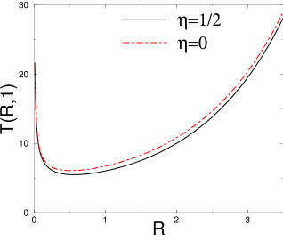
Figure 1: Mean first-passage time $T(R,\xi=1)$ vs. $R$ given respectively in Eq. (50) for $\eta=1/2$ (solid (black) line) and in Eq. (91) for $\eta=0$ (dot-dashed (red) line). For convenience, we have set the parameter $\xi=1$ for both $\eta=1/2$ and $\eta=0$ and also $\gamma=1/2$ in both cases. Clearly, in both cases $T(R,1)$ has a unique minimum and also for all $R$, $T(R,1)$ for $\eta=1/2$ is always larger than $T(R,1)$ for $\eta=0$, indicating that the velocity randomization protocol i.e., $\eta=1/2$ is more efficient than position-only resetting ($\eta=0$).

Let us check the diffusive limit (29) in which case $\lambda\to(r/D)^{1/2}$ and

$$T(X_{r})\to\frac{{\rm e}^{X_{r}(r/D)^{1/2}}}{r}-\frac{1}{r}$$ (90)

recovering the result of [16].

In terms of the reduced variables $R$ (47) and $\xi$ (48) we obtain

$$2\gamma T(R,\xi) = -\frac{1}{R}+\frac{\left[{\rm e}^{(R(1+R))^{1/2}\xi}-R^{2}+R^{3/2}(1+R)^{1/2}\right]}{R(1+R-(R(1+R))^{1/2})}$$ (91)

which is to be compared with the $\eta=1/2$ case (50). As in the $\eta=1/2$ case, $T(R,\xi)$ as a function of $R$ for fixed $\xi$ has a unique minimum, signalling an optimal resetting rate (see Fig. (1) for a plot). We see that for the same values of the reduced variables, $T(R,\xi)$ is always greater for $\eta=0$ than for $\eta=1/2$. This shows that the velocity randomization protocol ($\eta=1/2$) is more efficient in searching for a fixed target than the position-only protocol ($\eta=0$), for the same parameter values such as $X_{r}$, $\gamma$ and $v_{0}$.

It is also useful to compare the optimal search time for the run-and tumble dynamics with reset, with the optimal search time for the purely diffusive search with reset. To make this comparison, we have to set the diffusion constant $D=v_{0}^{2}/(2\gamma)$ in the diffusive search. Setting $D=v_{0}^{2}/(2\gamma)$ in Eq. (46) and using $r=2\gamma R$ and $X_{r}=v_{0}\xi/(2\gamma)$, we get

$$2\gamma T_{\rm diff}(R,\xi)=\frac{e^{\sqrt{R}\,\xi}-1}{R}$$ (92)

which can be directly compared to Eq. (50) for $\eta=1/2$, or with Eq. (91) corresponding to $\eta=0$. Let us consider just the $\eta=1/2$ case which is the best possibility for run and tumble dynamics. For convenience, we set $\gamma=1/2$ and $\xi=1$ in both Eqs. (92) and (50) and optimize with respect to $R$. For the diffusive case, we get $R^{*}=2.53964\dots$ and the optimized mean search time is then

$$T_{\rm diff}(R^{*},\xi=1)=1.54414\cdots$$ (93)

In contrast, optimizing Eq. (50) (the $\eta=1/2$ case), we get $R^{*}=0.55873\cdots$ (see also Fig. 1). Correspondingly, the optimized mean search time is given by

$$T(R^{*},\xi=1)=5.48571\cdots>T_{\rm diff}(R^{*},\xi=1)=1.54414\cdots$$ (94)

Hence, the diffusive search with reset is certainly more efficient than the run and tumble dynamics with reset for the same set of parameters.

7 Conclusion

In this paper we have studied the resetting of a run and tumble particle in one dimension. First we derived the stationary state for resetting to point $X_{r}$ and simultaneous velocity resetting. It turns out that the stationary state does not depend on the resetting protocol. Indeed the stationary state distribution (26) has the same form as a diffusive process under resetting. The width of the stationary distribution decreases with $\gamma$ and thus increases with increasing velocity correlation time.

However the velocity resetting protocol does affect the survival probability in the presence of an absorbing target at the origin. We have derived explicit expressions for the mean time to absorption in the case of position resetting and velocity randomization (50) and position-only resetting (91). For other parameters fixed, the position-only resetting gives a greater mean time to absorption. Writing the mean time to absorption in terms of the reduced variables $R$ (47) and $\xi$ (48) we see that there is an optimal value of $R$ which minimises the mean time to absorption. It would be of interest to consider how these results generalise to the case of partial absorption of the particle by the boundary [57, 14].

Throughout we have used a renewal equation approach which facilitates the calculations. It would be interesting to see how this approach can be extended to study the resetting of a run and tumble particle in higher dimensions.

It would also be of interest to consider the resetting of other stochastic processes with correlated noise. For example, physical Brownian motion is described as an Ornstein-Uhlenbeck process [1]

$$\frac{{\rm d}x}{{\rm d}t}=v\\ \frac{{\rm d}v}{{\rm d}t}=-\gamma v+\eta(t)$$ (95)

where $\eta(t)$ is usual white noise. The renewal approach should again be applicable in this case.

Finally, we speculate that progress in manipulating bacteral swimming dynamics with light (see e.g. [58, 59]) may allow future experimental protocols that approximate to velocity resetting.

References

References

• [1] Uhlenbeck G E and Ornstein L S 1930 On the Theory of the Brownian Motion Phys. Rev. 36, 823
• [2] Hagan P S, Doering C R, Levermore C D 1989 The distribution of exit times for weakly colored noise J. Stat. Phys. 54, 1321–1352
• [3] Weiss G H 2002 Some applications of persistent random walks and the telegrapher’s equation. Physica A 311 381
• [4] S. Herrmann and P. Vallois 2010 From persistent random walk to the telegraph noise Stoch. Dyn. 10, 161.
• [5] Wu H, Li B-L, Springer T A, Neill W H 2000 Modelling animal movement as a persistent random walk in two dimensions: expected magnitude of net displacement Ecological Modelling 132, 115-124
• [6] Tejedor, V., Voituriez, R. and BΓ©nichou, O. 2012 Optimizing persistent random searches. Phys. Rev. Lett. 108, 088103
• [7] Bhat D and Gopalakrishnan M 2013 Memory, bias, and correlations in bidirectional transport of molecular-motor-driven cargoes. Phys. Rev. E 88 042702
• [8] Detcheverry F 2015 Non-Poissonian run-and-turn motions, Europhys. Lett. 111 60002
• [9] Rosenau P 1993 Random walker and the telegrapher’s equation: A paradigm of a generalized hydrodynamics Phys. Rev. E 48, R655(R)
• [10] Elgeti J and Gompper G 2015, Run-and-tumble dynamics of self-propelled particles in confinement, Europhys. Lett. 109 58003
• [11] Angelani L 2017 Confined run-and-tumble swimmers in one dimension J. Phys. A: Math. Theor. 50 325601.
• [12] Slowman A B, Evans M R, and Blythe R A 2016 Jamming and Attraction of Interacting Run-and-Tumble Random Walkers Phys. Rev. Lett. 116, 218101
• [13] Slowman A B, Evans M R, and Blythe R A 2017 Exact solution of two interacting run-and-tumble random walkers with finite tumble duration J. Phys. A: Math. Theor 50, 375601
• [14] Angelani L 2015. Run-and-tumble particles, telegrapher’s equation and absorption problems with partially reflecting boundaries. J. Phys. A: Math. Theor. 48 495003.
• [15] Malakar K et al 2018 Steady state, relaxation and first-passage properties of a run-and-tumble particle in one- dimension J. Stat. Mech. 043215
• [16] Evans M R and Majumdar S N 2011 Diffusion with stochastic resetting, Phys. Rev. Lett. 106, 160601
• [17] Manrubia S C and Zanette D H 1999 Stochastic multiplicative processes with reset events, Phys. Rev. E 59, 4945
• [18] Montero M, MasΓ³-Puigdellosas A, Villarroel J 2017 Continuous-time random walks with reset events: Historical background and new perspectives European Physical Journal B 90 176
• [19] Evans M R and Majumdar S N 2011 Diffusion with optimal resetting, J. Phys. A: Math. Theor. 44, 435001
• [20] Evans M R and Majumdar S N 2014 Diffusion with resetting in arbitrary spatial dimension J. Phys. A: Math. Theor. 47, 285001
• [21] Majumdar S N, Sabhapandit S and Schehr G 2015, Dynamical transition in the temporal relaxation of stochastic processes under resetting Phys. Rev. E 91 052131
• [22] BΓ©nichou O, Loverdo C, Moreau M, and Voituriez R 2011, Intermittent search strategies, Rev. Mod. Phys. 83, 81.
• [23] Montanari A and Zecchina R 2002, Optimizing searches via rare events, Phys. Rev. Lett. 88, 178701
• [24] Eule S and Metzger J J 2016 Non-equilibrium steady states of stochastic processes with intermittent resetting New J. Phys. 18, 033006
• [25] Pal A, Kundu A and Evans M R 2016 Diffusion under time-dependent resetting J. Phys. A: Math. Theor. 49, 225001
• [26] Nagar A and Gupta S 2016 Diffusion with stochastic resetting at power-law times Phys. Rev. E 93, 060102 (R)
• [27] Bhat U, De Bacco C, Redner S 2016 Stochastic Search with Poisson and Deterministic Resetting J. Stat. Mech. P083401
• [28] Husain K and Krishna S 2016 Efficiency of a Stochastic Search with Punctual and Costly Restarts Preprint arXiv: 1609.03754
• [29] Pal A and Reuveni S 2017 First Passage under Restart Phys. Rev. Lett. 118 030603
• [30] Boyer D and Solis-Salas C 2014 Random walks with preferential relocations to places visited in the past and their application to biology Phys. Rev. Lett. 112, 240601
• [31] Majumdar SΒ N, Sabhapandit S and Schehr G 2015 Random walk with random resetting to the maximum position Phys. Rev. E 92, 052126
• [32] Boyer D, Evans M R and Majumdar S N 2017 Long time scaling behaviour for diffusion with resetting and memory J. Stat. Mech. P023208
• [33] Falcon-Cortes A, Boyer D, Giuggioli L, and Majumdar S N 2017 Localization transition induced by learning in random searches Phys. Rev. Lett. 119, 140603
• [34] Evans M R, Majumdar S N and Mallick K 2013 Optimal diffusive search: nonequilibrium resetting versus equilibrium dynamics J. Phys. A: Math. Theor 46 185001
• [35] Reuveni S 2016 Optimal stochastic restart renders fluctuations in first-passage times universal Phys. Rev. Lett. 116 170601
• [36] Bray A J, Majumdar S N and Schehr G 2013 Persistence and first-passage properties in nonequilibrium systems Adv. in Phys. 62 225
• [37] Kusmierz L, Majumdar S N, Sabhapandit S and Schehr G 2014 First order transition for the optimal search time of LΓ©vy flights with resetting Phys. Rev. Lett. 113 220602
• [38] Kusmierz L and Gudowska-Nowak E 2015 Optimal first-arrival times in LΓ©vy flights with restting Phys. Rev. E 92 052127
• [39] Campos D and MΓ©ndez V 2015 Phase transitions in optimal search times: How random walkers should combine reset- ting and flight scales Phys. Rev. E 92 062115
• [40] Christou C and Schadschneider A 2015 Diffusion with resetting in bounded domain J. Phys. A: Math. Theor. 48 285003
• [41] Gupta S, Majumdar S N and Schehr G 2014 Fluctuating interfaces subject to stochastic resetting, Phys. Rev. Lett. 112 220601
• [42] Durang X, Henkel M, Park H 2014 Statistical mechanics of the coagulation-diffusion process with a stochastic reset J. Phys. A: Math. Theor. 47 045002
• [43] Rothart T, Reuveni S and Urbakh M 2015 Michaelis-Menten reaction scheme as a unified approach towards the optimal restart problem Phys. Rev. E 92, 060101
• [44] Fuchs J, Goldt S and Seifert U 2016 Stochastic thermodynamics of resetting EPL 113 60009
• [45] Pal A and Rahav S 2017 Integral fluctuation theorems for stochastic resetting systems Phys. Rev. E 96 062135
• [46] Meylahn J M, Sabhapandit S, and Touchette H 2015 Large deviations of Markov processes with resetting Phys. Rev. E 92 062148
• [47] Harris R J and Touchette H 2017 Phase transitions in large deviations of reset processes J. Phys. A: Math. Theor. 50 10LT01
• [48] Hollander H D, Majumdar SN, Meylahn J M, and Touchette H 2018 Properties of additive functionals of Brownian motion with resetting preprint arXiv:1801.09909
• [49] Falcao R and Evans M R 2017 Interacting Brownian motion with resetting J. Stat. Mech. 023204
• [50] Pal A, Eliazar I, Reuveni S 2018 First passage under restart with branching preprint arXiv:1807.09363
• [51] Majumdar S N and Oshanin G 2018 Spectral content of fractional Brownian motion with stochastic reset J. Phys. A: Math. Theor. 51 435001
• [52] Mukherjee B, Sengupta K and Majumdar SN 2018 Quantum dynamics with stochastic reset preprint arXiv:1806.00019
• [53] Rose D C, Touchette H, Lesanovsky I and Garrhan J P 2018 Spectral properties of simple classical and quantum reset processes Phys. Rev. E 98, 022129
• [54] Chechkin A and Sokolov I M 2018 Random Search with Resetting: A Unified Renewal Approach Phys. Rev. Lett. 121 050601
• [55] Othmer H G, Dunbar S R, and Alt W 1988 Models of dispersal in biological systems J. Math. Biol. 26 263
• [56] Martens K, Angelani l, Di Leonardo R, and Bocquet L 2012 Probability distributions for the run-and-tumble bacterial dynamics: An analogy to the Lorentz model Eur. Phys. J. E 35, 84
• [57] Whitehouse J, Evans M R, and Majumdar S N 2013 Effect of partial absorption on diffusion with resetting Phys. Rev. E 87, 022118
• [58] Walter J M, Greenfield D, Bustamante C and Liphardt J 2007 Light-powering Escherichia coli with proteorhodopsin PNAS 104, 2408
• [59] Arlt J, Martinez V A, Dawson A, Pilizota T and Poon WCK 2018 Painting with light-powered bacteria Nat. Commun. 9, 768.