The full Schwinger-Dyson tower for random tensor models

Abstract:

We treat random rank-$D$ tensor models as $D$-dimensional quantum field theories—tensor field theories (TFT)—and review some of their non-perturbative methods. We classify the correlation functions of complex tensor field theories by boundary graphs, sketch the derivation of the Ward-Takahashi identity and stress its relevance in the derivation of the tower of exact, analytic Schwinger-Dyson equations for all the correlation functions (with connected boundary) of TFTs with quartic pillow-like interactions.

1 Introduction

In ordinary Quantum Field Theory (QFT) the Schwinger-Dyson equations account for the non-perturbative description of propagations and interactions, expressed in terms of equations of motion for the Green’s functions. Non-perturbative methods usually yield an infinite tower of coupled Schwinger-Dyson equations, which is rarely solvable. Some matrix models (or rather, matrix quantum field theories) [1] escape this feature, though. The solvability of the real quartic matrix model heavily (but not exclusively) relies on the $N^{2-2g}$-expansion of the Green’s functions in the matrix size, $N$, which allows to derive a closed equation for the two-point function in the planar ($g=0$) sector and thereafter to determine the higher-point functions by algebraic recursions. The extension of these non-perturbative approach to other kind of theories that also possess an inverse-$N$ expansion is therefore intriguing, since there it is natural to test for solvability, at least in the large-$N$ limit. To such family belong (random) tensor models.

The matrix model description of 2D-quantum gravity [2] inspired tensor models [3] and random tensors [4]. A colored structure on the tensors [5] led to their $1/N$-expansion. Beyond the random geometry and quantum gravity [6, 7, 8] applications that tensor models had, the large-number-of-particles limit of the Sachdev-Ye-Kitaev (SYK) [9] also unexpectedly received a tensor model description [10, 11, 12, 13, 14] and has become a tool in holography.

This short article only describes non-perturbative QFT aspects of (complex) tensor models; the reader is referred to the previous sources for a deeper physical approach.

For a scalar theory with cubic and quartic interactions, for sake of concreteness, the Schwinger-Dyson equations (SDE) are recursions that describe the insertions of the $n$-point and $(n+1)$-point functions into the $(n-1)$-point function one has then terms of the form (see e.g. [16] and [17, Fig. 1] ) The 1PI $2$-point function $\Gamma^{(2)}$, for instance, satisfies:

(1)

Due to the intricate combinatorics of the interaction vertices in matrix and tensor field theories (TFT), the analogue of equation (1) turns out to be more complicated. As a matter of fact, rank-$D$ tensor models have a propagator composed of $D$ parallel lines (nevertheless, denoted by A) each of which transmits momentum independently from the others, known as coloring (see Sec. 2 or [18, Fig. 2]). In particular, a quartic interaction vertex involves a choice of which of those colors are transmitted upwards, which downwards, which forwards in the small blob, $V$, of the sunset-term:

$$\raisebox{-0.435pt}{ \leavevmode\hbox to99.73pt{\vbox to50.07pt{\text{[drawing]}}}}\,\,.\qquad ? V ? V$$ (2)

For $D=3$ and the $2$-point function, notice that for the vertex $V$ of the sunset-diagram, the following might happen:

• $V$ can be any of $\{\raisebox{-0.322pt}{\includegraphics[height=9.90276pt]{gfx_S/3/Item4_VcvCT.pdf}}\}_{c=1,2,3}$ or $V=\leavevmode\hbox to11.11pt{\vbox to14.13pt{\text{[drawing]}}}$ for real or $\mathrm{O}(N)$ tensor models initiated by Carrozza and Tanasă [19], and used by Klebanov and Tarnopolsky [12] in the context of the SYK-like tensor models

• or $V=\raisebox{-0.322pt}{\includegraphics[height=9.04166pt]{graphs/3/Item4_Vcv.pdf}}$ for $c=1,2,3$ for complex or $\mathrm{U}(N)$ tensor models. The black-white bipartiteness reflects the presence of both the tensor field and its conjugate. Rather these $\mathrm{U}(N)$-invariant theories are the TFT we shall deal here with.

Higher-point functions follow an even more complicated schema. Either way, accordingly, the Green’s functions need further specification and, in fact, the classification of the correlation functions for higher-rank theories is the following:

• for real matrix theories, there are as many connected $k$-point functions [1] as integer partitions of $k$. Then, there are three $3$-point functions, five $4$-point functions, seven $5$-point functions, and so on.

• for complex tensor models the connected $k$-point functions are classified by (possibly disconnected) $D$-colored graphs in $k$ vertices [18]. In particular $k=2\ell$ should be even. Each edge in these graphs is of certain color $a$, and this enforces momentum-transmission of this very color. Therefore, the Feynman graph structures with four legs can encode momentum-transmission according to , , or (as pictured in Fig. 1) $\raisebox{-0.24pt}{\includegraphics[height=8.61108pt]{gfx_S/3/Item2_Melon.pdf}}\sqcup\raisebox{-0.24pt}{\includegraphics[height=8.61108pt]{gfx_S/3/Item2_Melon.pdf}}$ .

In particular, in order to obtain the analogue of eq. (1) in a $D$-dimensional QFT-context, say, for quartic tensor field theories of rank-$D$, one needs to specify which of the four $4$-point function we are inserting into the 2-point function. The aim of this paper is to explain how to achieve this and to arrive at analytic SDE for every (connected) correlation function. The methods exposed here are based on [18] and [21].

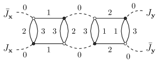
Figure 1: Connected 4-point $\varphi_{3}^{4}$-Feynman graph with disconnected boundary. The dashed (or $0$ color) transmits simultaneously the three colors. Hence, momentum transmission is encoded by $0a$-bicolored paths between external legs. This draws a graph, the boundary graph, which in this case is disconnected. Thus, this graph contributes to the $4$-point function $G^{(4)}_{\mathrm{m}|\mathrm{m}}$ or $G^{(4)}_{\mathrm{disconn.}}$ (see also Table 1 for notation).

Remark. We do not use Einstein’s implicit summation notation.

2 The strategy

The idea of the utilization of a matrix Ward identity (based on the Ward identity [22]) in order to derive the SDE of matrix models is due to Grosse and Wulkenhaar [1, 23].

2.1 Complex tensor models

Complex tensor models, colored tensor models and random tensor models [7] study fields $\varphi_{\mathbf{x}}\in\mathbb{C}$ ($\mathbf{x}\in I_{1}\times\ldots\times I_{D}\subset\mathbb{Z}^{D}$) whose indices transform independently under elements of $\mathrm{U}(N)$ of the product group $H_{D}=\mathrm{U}(N)^{D}$. This means that

$$\varphi_{x_{1}\ldots x_{D}} \mapsto\varphi^{\prime}_{x_{1}\ldots x_{D}}=\sum_{y_{a}}[W_{a}]_{x_{a}y_{a}}\varphi_{x_{1}\ldots y_{a}\ldots x_{D}}\,,\quad\bar{\varphi}_{x_{1}\ldots x_{D}}\mapsto\bar{\varphi}^{\prime}_{x_{1}\ldots x_{D}}=\sum_{y_{a}}[\overline{W}_{a}]_{x_{a}y_{a}}\bar{\varphi}_{x_{1}\ldots y_{a}\ldots x_{D}}\,,$$

for each $W_{a}$ in the $a$-th factor $\mathrm{U}(N)$ of $H_{D}$, for any $a=1,\ldots,D$. Each of the factors (and of the location of the tensor indices) is referred to as a color. Interactions of this kind of theories are $H_{D}$-invariants. We restrict to models for which any (graph)-vertex lies on a subgraph of the type for certain color $a$. For $D=3$, this constrains the interactions of models to the list

$$\raisebox{-0.322pt}{\includegraphics[height=9.90276pt]{graphs/3/Item4_Vav.pdf}},~{}\raisebox{-0.23pt}{\includegraphics[height=16.44719pt]{gfx_S/3B/Logo6_Q.pdf}}\,,~{}\raisebox{-0.23pt}{\includegraphics[height=20.23602pt]{gfx_S/3B/Item8_Q.pdf}}\,,~{}\raisebox{-0.23pt}{\includegraphics[height=24.97215pt]{gfx_S/3B/Item10_Q.pdf}}\,,~{}\raisebox{-0.23pt}{\includegraphics[height=29.7082pt]{gfx_S/3B/Item12_Q.pdf}}\,,\ldots(\mbox{for any color $a$}).$$ (3)

Other type of interactions need another methods. The origin of this restriction is technical and will be explained in Section 2.2. Here, we treat models with pillow-like interactions, but otherwise without any restriction in their rank. Pillows are melonic graphs of four vertices. These are $\{\raisebox{-0.322pt}{\includegraphics[height=9.90276pt]{graphs/3/Item4_V1v.pdf}},\raisebox{-0.322pt}{\includegraphics[height=9.90276pt]{gfx_S/3/Item4_V2v.pdf}},\raisebox{-0.322pt}{\includegraphics[height=9.90276pt]{gfx_S/3/Item4_V3v.pdf}}\},\mbox{ for rank-$3$ models, }\,\big{\{}\raisebox{-0.322pt}{\includegraphics[height=15.24158pt]{gfx_S/4/Icono4_V1v.pdf}},\raisebox{-0.322pt}{\includegraphics[height=15.24158pt]{gfx_S/4/Icono4_V2v.pdf}},\raisebox{-0.322pt}{\includegraphics[height=15.24158pt]{gfx_S/4/Icono4_V3v.pdf}},\raisebox{-0.322pt}{\includegraphics[height=15.24158pt]{gfx_S/4/Icono4_V4v.pdf}}\big{\}}$ for rank-$4$ models, etc. When the rank is clear, we denote by $V_{a}$ the pillow with preferred color $a$ (e.g. $\raisebox{-0.322pt}{\includegraphics[height=9.90276pt]{graphs/3/Item4_V1v.pdf}}=V_{1}$).

2.2 The usefulness of the Ward-Takahashi Identity

We consider the quartic tensor model with interaction $S_{\mathrm{int}}=\lambda\sum_{c=1}^{D}V_{c}$ with a kinetic Laplacian-like kernel $E$, which possibly breaks the $H_{D}$-symmetry in the quadratic invariant $\mathrm{Tr}_{2}(\bar{\varphi},\varphi)\to S_{0}=\mathrm{Tr}_{2}(\bar{\varphi},E\varphi)$. Functional integration of the partition function yields

$$Z[J,\bar{J};E]=C\exp\big{(}-\lambda\textstyle\sum{}_{\mathit{a}=1}^{3}V_{a}\big{)}\bigg{|}_{(\varphi,\bar{\varphi})\to(\frac{\delta}{\delta\bar{J}},\frac{\delta}{\delta J})}Z^{\mathrm{free}}[J,\bar{J};E]\,.$$

Any analytic Schwinger-Dyson equation begins by deriving with respect to the sources. By deriving with respect to $\bar{J}_{\mathbf{s}}$ we get [18, 21]

$$\frac{\delta\log Z[J,\bar{J};E]}{\delta\bar{J}_{\mathbf{s}}}=\frac{1}{E_{\mathbf{s}}}\bigg{\{}J_{\mathbf{s}}-\frac{1}{Z[J,\bar{J};E]}\bigg{(}\frac{\partial S_{\mathrm{int}}(\varphi,\bar{\varphi})}{\partial\bar{\varphi}_{\mathbf{s}}}\bigg{)}\bigg{|}_{(\varphi,\bar{\varphi})\to(\frac{\delta}{\delta\bar{J}},\frac{\delta}{\delta J})}Z[J,\bar{J};E]\bigg{\}}\,.$$ (4)

By assumption (Sec. 2.1), the term in round parenthesis contains, after evaluation of the sources, the subgraph , and thus a derivative of the form

$$\mathcal{L}_{m_{a}n_{a}}\equiv\sum\limits_{\mathbf{p}_{\hat{a}}\in\mathbb{Z}}\bigg{[}\frac{\delta^{2}Z[J,\bar{J};E]}{\delta J_{{p_{1}\ldots p_{a-1}m_{a}p_{a+1}\ldots p_{D}}}\delta\bar{J}_{{p_{1}\ldots p_{a-1}n_{a}p_{a+1}\ldots p_{D}}}}\bigg{]}$$ (5)

acted on by more derivatives. This term resembles the LHS appearing in the Ward-Takahashi Identity (WTI)

$$\sum\limits_{\mathbf{p}_{\hat{a}}\in\mathbb{Z}}\bigg{[}\frac{\delta^{2}Z[J,\bar{J};E]}{\delta J_{{p_{1}\ldots p_{a-1}m_{a}p_{a+1}\ldots p_{D}}}\delta\bar{J}_{{p_{1}\ldots p_{a-1}n_{a}p_{a+1}\ldots p_{D}}}}\times E_{m_{a}n_{a};\mathbf{p}_{\hat{a}}}\bigg{]}=D_{J,\bar{J}}\,Z[J,\bar{J};E]$$ (6)

obtained by Ousmane-Samary [25] from the $\mathrm{U}(N)$-invariance (this group being the $a$-th factor of $H_{D}$) of the path integral. Here, $E_{m_{a}n_{a};\mathbf{p}_{\hat{a}}}\equiv E_{p_{1}\cdots m_{a}\cdots p_{D}}-E_{p_{1}\cdots n_{a}\cdots p_{D}}$, $\mathbf{p}_{\hat{a}}\equiv(p_{1},\ldots,p_{a-1},p_{a+1},\ldots,p_{D})$ and $D_{J,\bar{J}}$ is a first order differential operator in the sources. It would be useful to reduce the derivatives by using this WTI; however, it also implies the difference of the kernels. We restrict, therefore, to models that satisfy that:

$$\mbox{for any color $a$, }\,\,\,E_{m_{a}n_{a};\mathbf{q}_{\hat{a}}}=E_{q_{1}\cdots m_{a}\cdots q_{D}}-E_{q_{1}\cdots n_{a}\cdots q_{D}}\mbox{ does not depend on $\mathbf{q}_{\hat{a}}$. } \diamondsuit$$ ()

We thus write only $E_{m_{a}n_{a};\mathbf{p}_{\hat{a}}}=:E_{m_{a}n_{a}}$ from now on. The condition $\diamondsuit$ ‣ 2.2 allows one to get the term $E_{m_{a}n_{a}}$ out of the sum and solve for $\mathcal{L}_{m_{a}n_{a}}$. We remark that the non-triviality of this task relies on the skew-symmetry of the indices of $E_{m_{a}n_{a}}$. This means that we need to find the term that is proportional to $\delta_{m_{a}n_{a}}$ in $\mathcal{L}_{m_{a}n_{a}}$ (see eq. (5)). This is a functional that we denote by $Y^{(a)}_{m_{a}}[J,\bar{J}\,]$ (and name, sloppily, $Y$-term). After complete knowledge about this $Y$-term has been obtained we say the WTI is full. The first full WTI was found for $\mathrm{O}(N)$ matrix models [1, Sec. 2].

3 The full Ward-Takahashi identity

For arbitrary rank-$D$ $\mathrm{U}(N)$ tensor models the full WTI reads [18]:

$$\!\!\!\!\!\mathcal{L}_{m_{a}n_{a}}=\left(\delta_{m_{a}n_{a}}Y^{(a)}_{m_{a}}[J,\bar{J}]\right)\,\cdot Z[J,\bar{J}\,;E]+\sum\limits_{\mathbf{p}_{\hat{a}}\in\mathbb{Z}^{D-1}}\frac{1}{E_{m_{a}n_{a}}}\left(\bar{J}_{m_{a}\mathbf{p}_{\hat{a}}}\frac{\delta}{\delta\bar{J}}_{n_{a}\mathbf{p}_{\hat{a}}}-J_{n_{a}\mathbf{p}_{\hat{a}}}\frac{\delta}{\delta J}_{m_{a}\mathbf{p}_{\hat{a}}}\right)Z[J,\bar{J};E]\,.$$

In the next subsections, we explain how to define the correlation functions, and, subsequently, how to obtain the $Y$-term.

3.1 The expansion of the free energy in boundary graphs

The (connected) correlation functions of TFTs will be defined as derivatives with respect to sources, as in usual QFT. Nevertheless, the naive Ansatz

$$\log Z[J,\bar{J}] \stackrel{{\scriptstyle?}}{{=}}\sum_{\mathbf{x},\mathbf{y}}G^{(2)}(\mathbf{x},\mathbf{y})J_{y_{1}y_{2}y_{3}}\bar{J}_{x_{1}x_{2}x_{3}}+\sum_{\mathbf{w},\mathbf{x},\mathbf{y},\mathbf{z}}G^{(4)}(\mathbf{w},\mathbf{x},\mathbf{y},\mathbf{z})J_{x_{1}x_{2}x_{3}}\bar{J}_{w_{1}w_{2}w_{3}}J_{y_{1}y_{2}y_{3}}\bar{J}_{z_{1}z_{2}z_{3}}+\mathcal{O}(4)\,$$

is, due to the color structure, an oversimplification that impairs the derivation of analytic Schwinger-Dyson equations for the thus defined $G^{(2\ell)}$-functions. The right expansion takes into account the transmission of momentum inside classes of Feynman graphs, and is given by

$$\log Z[J,\bar{J}] =\sum_{\mathbf{x}}G^{(2)}(\mathbf{x})J_{x_{1}x_{2}x_{3}}\bar{J}_{x_{1}x_{2}x_{3}}+\sum_{\mathbf{x},\mathbf{y}}G^{(4)}_{\mathrm{disconn.}}(\mathbf{x},\mathbf{y})J_{x_{1}x_{2}x_{3}}\bar{J}_{x_{1}x_{2}x_{3}}J_{y_{1}y_{2}y_{3}}\bar{J}_{y_{1}y_{2}y_{3}}$$ (7)

$$+\sum_{\mathbf{x},\mathbf{y}}G^{(4)}_{1}(\mathbf{x},\mathbf{y})J_{y_{1}y_{2}y_{3}}\bar{J}_{x_{1}y_{2}y_{3}}J_{x_{1}x_{2}x_{3}}\bar{J}_{y_{1}x_{2}x_{3}}+\sum_{\mathbf{x},\mathbf{y}}G^{(4)}_{2}(\mathbf{x},\mathbf{y})J_{y_{1}y_{2}y_{3}}\bar{J}_{y_{1}x_{2}y_{3}}J_{x_{1}x_{2}x_{3}}\bar{J}_{x_{1}y_{2}x_{3}}$$

$$+\sum_{\mathbf{x},\mathbf{y}}G^{(4)}_{3}(\mathbf{x},\mathbf{y})J_{y_{1}y_{2}y_{3}}\bar{J}_{x_{1}x_{2}y_{3}}J_{x_{1}x_{2}x_{3}}\bar{J}_{y_{1}y_{2}x_{3}}+\mathcal{O}(6)$$

The sub-indices of the 4-point functions $G^{(4)}$ will be clear soon. This expansion can be conveniently (compactly) organized by, again, colored graphs. This would yield an algorithmic derivation of the $Y$-term. Notice the effect of the the double derivative on the source-term

$$\sum_{\mathbf{p}_{\hat{a}}}\frac{\delta}{\delta J_{m_{a}\mathbf{p}_{\hat{a}}}}\frac{\delta}{\delta\bar{J}_{n_{a}\mathbf{p}_{\hat{a}}}}\,\,\sum_{\mathbf{x}^{1},\cdots,\mathbf{y},\cdots\mathbf{x}^{\ell}}G^{(2\ell)}(\mathbf{x}^{1},\ldots,\mathbf{y},\ldots\mathbf{x}^{\ell})[J_{\mathbf{x}^{1}}\cdots J_{\mathbf{y}}\cdots J_{\mathbf{x}^{\ell}}]\cdot[\bar{J}_{\cdots}\cdots\bar{J}_{\ldots y_{a}\ldots}\cdots\bar{J}_{\cdots}\,]\,.$$ (8)

Namely, from this equation it is clear that $Y_{m_{a}}^{(a)}$ has contributions from ‘hitting’ two sources $J$ and $\bar{J}$ that are connected by an $a$-colored edge in the boundary graph (in this term, as a matter of fact, $\bar{J}_{\ldots y_{a}\ldots}$ and $J_{\mathbf{y}}$). In order to understand this, we find convenient to recall what happens in the for matrix field theories. If this is superfluous for the reader, Sec. 3.1.1 could be skipped.

3.1.1 The free energy for real matrix models

As pointed out in the introduction, the correlation functions (the momenta of the free energy $\log Z_{\mathrm{matrix}}$) of a general real matrix model are classified by integer partitions of $k$. If these partitions are indexed by $\alpha\in\{1,\ldots,P(k)\}$), the free energy is expanded as

$$\log Z_{\mathrm{matrix}}[J]=\sum_{k=1}^{\infty}\sum_{\alpha=1}^{P(k)}\frac{1}{\sigma(\alpha)}G^{(k)}_{\alpha}\star\hskip 2.0pt\mbox{{{j}}}(\alpha)=\mbox{`sum over triangulation of boundaries (circles)'}.$$ (9)

This is shorthand but is not a formal expression. An integer partition $\alpha=(n_{1},\ldots,n_{B(\alpha)})\in\mathbb{Z}_{\geq 0}$ of $k$ (i.e. $k=\sum_{r=1}^{B(\alpha)}n_{r}$ with $n_{B(\alpha)}\neq 0$, and $n_{i}<n_{j}$ if $i<j$) determines $B(\alpha)$ boundaries, $n_{r}$ of which carry $r$ sources attached. Thus, $(\hskip 2.0pt\mbox{{{j}}}(\alpha))(\mathbf{p}^{1},\ldots,\mathbf{p}^{B(\alpha)}):=\prod_{r=1}^{B(\alpha)}J_{p_{1}^{r}p_{2}^{r}}J_{p_{2}^{r}p_{3}^{r}}\cdots J_{p_{n_{r}}^{r}p_{1}^{r}}$ and $\mathbf{p}^{r}=(p^{1}_{1},\ldots,p_{n_{r}}^{r})$. The star, $\star\,$, point-wise sums the product $(G_{\alpha}^{(k)}\cdot\hskip 2.0pt\mbox{{{j}}}(\alpha))$ is over the arguments $(\mathbf{p}^{1},\ldots,\mathbf{p}^{B(\alpha)})$. Further, $\sigma(\alpha)$ is a symmetry factor.

The topological significance of this expansion is clear: Equation (9) is a sum over triangulations of the boundary of the surfaces that the ribbon graphs triangulate. That is, $\alpha$ determines for $n_{r}$ circles a precise ‘triangulation by $r$ intervals’. Based on this, one can derive the free energy for complex tensor models. The useful concept there is that of a boundary graph.

3.1.2 The free energy of complex tensor models

The expansion of the free energy also has a geometrical meaning. It is an expansion over all triangulations of boundaries, but in higher dimensions. For $D=3$, these are triangulations of closed, orientable surfaces. In fact, these are triangulable by bipartite $3$-colored graphs and the sum turns out to be over all the boundary graph that are triangulated by a particular model $S_{\mathrm{int}}$. The boundaries are characterized in [18]. The general expansion for any rank reads:

$$\log Z_{\,\,\mathrm{tensors}}[J,\bar{J};E] =\sum\limits_{\ell=1}^{\infty}\sum\limits_{\begin{subarray}{c}\mathcal{B}\,\mathrm{is\,\,boundary\,of\,}S_{\mathrm{int}}\\ \#\mathrm{Vertices}(\mathcal{B})=2\ell\end{subarray}}\frac{1}{|\mathrm{Aut}_{\mathrm{c}}(\mathcal{B})|}G^{(2\ell)}_{\mathcal{B}}\star\hskip 2.0pt\mbox{{{j}}}(\mathcal{B})\,.$$ (10)

The elements of this formula are:

• to each boundary graph $\mathcal{B}$,  j associates a function $\hskip 2.0pt\mbox{{{j}}}(\mathcal{B}):M_{D\times\ell}(\mathbb{Z})\to\mathbb{C}$ in the sources given by

  $$(\hskip 2.0pt\mbox{{{j}}}(\mathcal{B}))(\mathbf{X})\equiv\prod_{\alpha=1}^{\ell}J_{\mathbf{x}^{\alpha}}\bar{J}_{\mathbf{y}^{\alpha}(\mathbf{X})},\mbox{being $\mathbf{x}^{\alpha}$, ($\alpha=1,\ldots,\ell$) the columns of $\mathbf{X}\,$,}$$ (11)

  and $\{\mathbf{y}^{\alpha}(\mathbf{X})\}_{\alpha}$ is the set of (unordered) momenta $\mathbf{y}^{\alpha}$ that one gets in the $\bar{J}$-sources at the external legs of a Feynman graph $\mathcal{G}$ with $\partial\mathcal{G}=\mathcal{B}$ by ‘injecting momenta the ${\mathbf{x}^{\gamma}}$’ ($\gamma=1,\ldots,\ell$) at the external legs marked by $J$-sources (see Fig. 1). We choose the notation $\mathcal{B}_{*}(\mathbf{X})=(\mathbf{y}^{1},\ldots,\mathbf{y}^{\ell})$ (see [18] for the detailed construction). For instance, $\hskip 2.0pt\mbox{{{j}}}(\raisebox{-0.322pt}{\includegraphics[height=9.90276pt]{graphs/3/Item4_V1v.pdf}})(\mathbf{x},\mathbf{z})=J_{z_{1}z_{2}z_{3}}\bar{J}_{x_{1}z_{2}z_{3}}J_{x_{1}x_{2}x_{3}}\bar{J}_{z_{1}x_{2}x_{3}}$, since $(\raisebox{-0.322pt}{\includegraphics[height=9.90276pt]{graphs/3/Item4_V1v.pdf}})_{*}(\mathbf{x},\mathbf{z})=(x_{1},z_{2},z_{3}\,,\,z_{1},x_{2},x_{3})$

• one then sums the product $G^{(2\ell)}_{\mathcal{B}}(\mathbf{X})\cdot(\hskip 2.0pt\mbox{{{j}}}(\mathcal{B}))(\mathbf{X})$ over all momenta $\mathbf{X}\in M_{D\times\ell}(\mathbb{Z})$; the star $\star$ abbreviates this sum

• finally, one divides by the order of the automorphism group $\mathrm{Aut}_{\mathrm{c}}(\mathcal{B})$ of the graph $\mathcal{B}$. The automorphism group will be important in the following section.

Table 1: Correlation functions of the $\varphi^{4}_{3}$-theory until order six

Since from now on we work only with TFTs, we omit the subindex ‘tensors’ in the partition function $Z_{\mathrm{tensors}}$. For rank-$3$ models, the most general expansion is

$$\log Z[J,\bar{J}\,] =G^{(2)}\star\hskip 2.0pt\mbox{{{j}}}(\mathrm{m})+\frac{1}{2!}G^{(4)}_{\hskip 0.2pt\mathrm{m}|\hskip 0.2pt\mathrm{m}}\star\hskip 2.0pt\mbox{{{j}}}(\hskip 0.2pt\mathrm{m}|\hskip 0.2pt\mathrm{m})+\frac{1}{2}\sum_{c=1}^{3}\bigg{[}G^{(4)}_{V_{c}}\star\hskip 2.0pt\mbox{{{j}}}\big{(}\,V_{c}\,\big{)}+\frac{1}{3}G^{(6)}_{Q_{c}}\star\hskip 2.0pt\mbox{{{j}}}(Q_{c})+G^{(6)}_{F_{c}}\star\hskip 2.0pt\mbox{{{j}}}(F_{c})$$

$$\,\,\,\,\,\,\,+\frac{1}{2}G^{(6)}_{\mathrm{m}\hskip 0.2pt|\hskip 0.2ptV_{c}}\star\hskip 2.0pt\mbox{{{j}}}(\mathrm{m}\hskip 0.2pt|\hskip 0.2ptV_{c})\bigg{]}+\frac{1}{3}G^{(6)}_{K_{3,3}}\star\hskip 2.0pt\mbox{{{j}}}(K_{3,3})+\frac{1}{3!}G^{(6)}_{\hskip 0.2pt\mathrm{m}|\hskip 0.2pt\mathrm{m}|\hskip 0.2pt\mathrm{m}\hskip 0.2pt}\star\hskip 2.0pt\mbox{{{j}}}(\hskip 0.2pt\mathrm{m}|\hskip 0.2pt\mathrm{m}|\hskip 0.2pt\mathrm{m}\hskip 0.2pt)+\mathcal{O}(8)\,.$$ (12)

As shown in [18] (relying on [26]) for rank-$D$ models with all the pillows $S_{\mathrm{int}}=\lambda\sum_{c=1}^{D}V_{c}$, for any $D$-colored graph $\mathcal{B}$, even if $\mathcal{B}$ is disconnected, $G^{(2\ell)}_{\mathcal{B}}\equiv\!\!\!\!\!\!\!/\,\,\,\,0$ holds. Table 1 shows the transition from the original source [18] notation to the compact one used here.

3.2 Graph calculus

The free energy is generated by graphs. Since this is not a formal expansion, a tool should be developed in order to read off the coefficients (functions) of the graphs. This is the graph calculus [18], which consists in deriving functionals $\mathcal{A}[J,\bar{J}\,]$ with respect to $(\hskip 2.0pt\mbox{{{j}}}(\mathcal{B}))(\mathbf{X})$, where $\mathcal{B}$ is a boundary graph, and by momenta $\mathbf{X}=(\mathbf{x}^{1},\ldots,\mathbf{x}^{\ell})$ ($2\ell=\#$ vertices of $\mathcal{B}$). We restrict $\mathbf{X}$ to

$$\mathcal{F}_{D,\ell}:=\{(\mathbf{x}^{1},\ldots,\mathbf{x}^{\ell})\in M_{D\times\ell}(\mathbb{Z})\,|\,x^{\alpha}_{c}\neq x^{\nu}_{c}\,\,\mbox{ if }\alpha\neq\nu\,(\alpha,\nu=1,\ldots,\ell),\mbox{ for all }c=1,\ldots,D\}\,,$$

the space of momenta away from the ‘colored diagonals’. One then sets $\partial\mathcal{A}[J,\bar{J}\,]/\partial\mathcal{B}$ to be the function that at $\mathbf{X}\in\mathcal{F}_{D,\ell}$ takes the value

$$\frac{\delta^{2\ell}\mathcal{A}[J,\bar{J}\,]}{\delta\hskip 2.0pt\mbox{{{j}}}(\mathcal{B})(\mathbf{X})}\bigg{|}_{J=\bar{J}=0}.$$

An important result is the independence of graphs, meaning that if $\mathcal{C}$ is another graph $\partial\mathcal{C}/\partial\mathcal{B}$ is non-zero only if the graphs $\mathcal{B}$ and $\mathcal{C}$ are isomorphic. If that is the case, the derivative $\partial\mathcal{C}/\partial\mathcal{B}$ is found to be a group action by $\mathrm{Aut}_{\mathrm{c}}(\mathcal{B})$. Concretely, if $\mathbf{C}=(\mathbf{c}^{1},\ldots,\mathbf{c}^{k})\in M_{D\times k}(\mathbb{Z})$ and $\mathbf{X}\in\mathcal{F}_{D,\ell}$,

$$\frac{\partial\mathcal{C}(\mathbf{C})}{\partial\mathcal{B}(\mathbf{X})}=\begin{cases}\delta_{\ell k}\cdot\Big{(}\displaystyle\sum\limits_{\hat{\sigma}\in\mathrm{Aut}_{\mathrm{c}}(\mathcal{B})}\delta^{\mathbf{c}^{\sigma(1)},\ldots,\mathbf{c}^{\sigma(k)}}_{\mathbf{x}^{1},\mathbf{x}^{2},\ldots,\mathbf{x}^{\ell}}\Big{)}&\qquad\mbox{if }\,\,\,\mathcal{B}\cong\mathcal{C}\,,\\ \,\,\,\quad 0&\qquad\mbox{if }\,\,\mathcal{B}\ncong\mathcal{C}\,.\end{cases}$$

where $\hat{\sigma}\in\mathrm{Aut}_{\mathrm{c}}(\mathcal{B})$ denotes the lift of a permutation $\sigma\in\mathrm{Sym}(\ell)$ to the corresponding element of the automorphism group $\mathrm{Aut}_{\mathrm{c}}(\mathcal{B})$. Now we are in position to define the correlation functions by

$$G_{\mathcal{B}}^{(2\ell)}\equiv\frac{\partial\log Z[J,\bar{J}\,;E]}{\partial\mathcal{B}}\,\,.$$ (13)

Example 3.1 (Meaning of $\partial/\partial\hskip 1.0pt\raisebox{-0.12pt}{\includegraphics[width=8.61108pt]{graphs/3/Item6_K33.pdf}}$).

If $\mathcal{A}[J,\bar{J}\,]$ is a functional and $\mathbf{X}=(\mathbf{x}^{1},\mathbf{x}^{2},\mathbf{x}^{3})\in\mathcal{F}_{3,3}$, one has

$$\frac{\partial\mathcal{A}[J,\bar{J}\,]}{\partial\hskip 1.0pt\raisebox{-0.12pt}{\includegraphics[width=8.61108pt]{graphs/3/Item6_K33.pdf}}}(\mathbf{X})=\frac{\delta^{6}\mathcal{A}[J,\bar{J}\,]}{\delta J_{\mathbf{x}^{1}}\delta J_{\mathbf{x}^{2}}\delta J_{\mathbf{x}^{3}}\delta\bar{J}_{\mathbf{y}^{1}}\delta\bar{J}_{\mathbf{y}^{2}}\delta\bar{J}_{\mathbf{y}^{3}}}\bigg{|}_{J=0=\bar{J}}=\frac{\delta^{6}\mathcal{A}[J,\bar{J}\,]}{\delta J_{\mathbf{x}^{1}}\delta J_{\mathbf{x}^{2}}\delta J_{\mathbf{x}^{3}}\delta\bar{J}_{x^{1}_{1}x^{2}_{2}x^{3}_{3}}\delta\bar{J}_{x^{2}_{1}x^{3}_{2}x^{1}_{3}}\delta\bar{J}_{x^{3}_{1}x^{1}_{2}x^{2}_{3}}}\bigg{|}_{J=0=\bar{J}}\,\,,$$

since

$$(\hskip 1.0pt\raisebox{-0.2pt}{\includegraphics[width=12.18468pt]{graphs/3/Item6_K33.pdf}})_{*}\{\mathbf{x}^{1},\mathbf{x}^{2},\mathbf{x}^{3}\}=\{\mathbf{y}^{1},\mathbf{y}^{2},\mathbf{y}^{3}\}=\bigg{\{}\bigg{[}\begin{smallmatrix}x^{1}_{1}\\ x_{2}^{2}\\ x_{3}^{3}\end{smallmatrix}\bigg{]},\bigg{[}\begin{smallmatrix}x^{2}_{1}\\ x_{2}^{3}\\ x_{3}^{1}\end{smallmatrix}\bigg{]},\bigg{[}\begin{smallmatrix}x^{3}_{1}\\ x_{2}^{1}\\ x_{3}^{2}\end{smallmatrix}\bigg{]}\bigg{\}}\,.$$

The effect of the operator $\partial/\partial\hskip 1.0pt\raisebox{-0.12pt}{\includegraphics[width=8.61108pt]{graphs/3/Item6_K33.pdf}}$ acting on the free energy is to generate a boundary-torus, since is a graph triangulating $\mathbb{T}^{2}$. The double action of (say) $\partial^{2}/\partial\hskip 1.0pt\raisebox{-0.12pt}{\includegraphics[width=8.61108pt]{graphs/3/Item6_K33.pdf}}\hskip 1.0pt\partial\hskip 1.0pt\raisebox{-0.24pt}{\includegraphics[height=8.61108pt]{gfx_S/3/Item2_Melon.pdf}}$ on $\log Z$ —denoted by $G^{(8)}_{\raisebox{-0.2pt}{\includegraphics[height=4.52083pt]{gfx_S/3/Item2_Melon.pdf}}\hskip 1.0pt|\hskip 1.0pt\raisebox{-0.12pt}{\includegraphics[width=6.02777pt]{graphs/3/Item6_K33.pdf}}}$ according to eq. (13) — is to select, from among all the spaces generated by the tensor model in question, only the bordisms from the sphere to the torus, that respect the particular triangulation given by and .

3.3 The Y-term

From the given expansion of the free energy one can derive the $Y$-term. In order to do so, we need to introduce the functions $\Delta_{m_{a},r}G_{\mathcal{B}}^{(2\ell)}$. These are the coefficients in eq. (8), after hitting the $r$-th white vertex $\mathbf{x}^{r}$ and the vertex $\mathbf{y}^{\mu(r,a)}$ connected to it by a $a$-colored vertex in the boundary graph. To wit, when the two derivatives act on $J_{\mathbf{x}^{r}}$ and $\bar{J}_{\ldots x^{r}_{a}\ldots}$ in

$$\sum_{\mathbf{p}_{\hat{a}}}\frac{\delta}{\delta J_{m_{a}\mathbf{p}_{\hat{a}}}}\frac{\delta}{\delta\bar{J}_{n_{a}\mathbf{p}_{\hat{a}}}}\,\,\sum_{\mathbf{x}^{1},\cdots,\mathbf{x}^{r},\cdots\mathbf{x}^{\ell}}G^{(2\ell)}_{\mathcal{B}}(\mathbf{x}^{1},\ldots,\mathbf{x}^{r},\ldots\mathbf{x}^{\ell})[J_{\mathbf{x}^{1}}\cdots J_{\mathbf{x}^{r}}\cdots J_{\mathbf{x}^{\ell}}]\cdot[\bar{J}_{\cdots}\cdots\bar{J}_{\ldots x^{r}_{a}\ldots}\cdots\bar{J}_{\cdots}\,]\,,$$ (14)

two vertices of the boundary graph are removed. The surviving sources have then the form

$$(\hskip 2.0pt\mbox{{{j}}}(\mathcal{B}\ominus e^{r}_{a}))(\mathbf{x}^{1},\ldots,\widehat{\mathbf{x}}^{r},\ldots,\mathbf{x}^{\ell})$$

for certain residual graph denoted by $\mathcal{B}\ominus e^{r}_{a}$. Its coefficient is the function $\delta_{m_{a}n_{a}}\Delta_{m_{a},r}G_{\mathcal{B}}^{(2\ell)}$, by definition of $\Delta_{m_{a},r}$. Notice that $\Delta_{m_{a},r}G_{\mathcal{B}}^{(2\ell)}$ has $\ell-1$ arguments in $\mathbb{Z}^{D}$. In this notation, the explicit $Y$-term consequently reads [18]:

$$Y^{(a)}_{m_{a}}[J,\bar{J}] =\sum\limits_{q_{c},q_{b}}G^{(2)}(m_{a},q_{c},q_{b})+\frac{1}{2}\sum\limits_{r=1}^{2}\big{(}\Delta_{m_{a},r}G^{(4)}_{\mathrm{m}\hskip 0.2pt|\hskip 0.2pt\mathrm{m}}+\sum_{i=1}^{3}\Delta_{m_{a},r}G^{(4)}_{i}\big{)}\star\hskip 2.0pt\mbox{{{j}}}\big{(}\mathrm{m}\big{)}$$

$$\,\,+\frac{1}{3}\sum\limits_{r=1}^{3}\sum\limits_{i=1}^{3}\big{(}\Delta_{m_{a},r}G^{(6)}_{Q_{i}}\big{)}\star\hskip 2.0pt\mbox{{{j}}}\big{(}V_{i}\,\big{)}+\frac{1}{3}\sum_{r=1}^{3}(\Delta_{m_{a},r}G^{(6)}_{K_{3,3}})\star\hskip 2.0pt\mbox{{{j}}}\big{(}V_{a}\big{)}$$

$$\,\,+\sum\limits_{c\neq a}\Big{\{}\big{(}\Delta_{m_{a},1}G^{(6)}_{F_{c;ba}}\big{)}\star\hskip 2.0pt\mbox{{{j}}}\big{(}V_{b}\big{)}+\big{(}\Delta_{m_{a},2}G^{(6)}_{F_{c;ba}}\big{)}\star\hskip 2.0pt\mbox{{{j}}}\big{(}V_{b}\big{)}$$ (15)

$$\,\,+\big{(}\Delta_{m_{a},3}G^{(6)}_{F_{c;ba}}\big{)}\star\hskip 2.0pt\mbox{{{j}}}\big{(}V_{a}\big{)}\Big{\}}+\big{(}\Delta_{m_{a},1}G^{(6)}_{F_{a;bc}}\big{)}\star\hskip 2.0pt\mbox{{{j}}}\big{(}V_{c}\big{)}+\big{(}\Delta_{m_{a},2}G^{(6)}_{F_{a;bc}}\big{)}\star\hskip 2.0pt\mbox{{{j}}}\big{(}\vspace{.3pt}\mathrm{m}\vspace{.3pt}|\vspace{.3pt}\mathrm{m}\vspace{.3pt}\big{)}$$

$$\,\,+\big{(}\Delta_{m_{a},3}G^{(6)}_{F_{a;bc}}\big{)}\star\hskip 2.0pt\mbox{{{j}}}\big{(}V_{b}\big{)}+\frac{1}{3!}\sum\limits_{r=1}^{3}\big{(}\Delta_{m_{a},r}G^{(6)}_{\mathrm{m}\hskip 0.2pt|\hskip 0.2pt\mathrm{m}|\hskip 0.2pt\mathrm{m}}\big{)}\star\hskip 2.0pt\mbox{{{j}}}\big{(}\vspace{.3pt}\mathrm{m}\vspace{.3pt}|\vspace{.3pt}\mathrm{m}\vspace{.3pt}\big{)}$$

$$\,\,+\sum_{i=1,2,3}\Big{\{}\frac{1}{2}\big{(}\Delta_{m_{a},1}G^{(6)}_{\hskip 0.2pt\mathrm{m}|\hskip 0.2ptV_{i}}\big{)}\star\hskip 2.0pt\mbox{{{j}}}\big{(}V_{i}\big{)}+\frac{1}{2}\sum\limits_{r=2,3}\big{(}\Delta_{m_{a},r}G^{(6)}_{\hskip 0.2pt\mathrm{m}|\hskip 0.2ptV_{i}}\big{)}\star\hskip 2.0pt\mbox{{{j}}}\big{(}\vspace{.3pt}\mathrm{m}\vspace{.3pt}|\vspace{.3pt}\mathrm{m}\vspace{.3pt}\big{)}\Big{\}}+\mathcal{O}(6)\,.$$

the notation $F_{a;bc}$ means the graph $F_{a}=\raisebox{-0.45pt}{\includegraphics[height=12.91663pt]{gfx_S/3/Item6_Eabcs.pdf}}$ ($b\neq a\neq c\neq b$) with a left-to-right ordering of the white vertices. Also, the graph-subindex notation (i.e. switching back to the left columns of Table 1) might be helpful in order to understand how this expression was computed.

4 The tower of Schwinger-Dyson equations (connected boundary)

With the $Y$-term known, it is clear that one can express it as a sum over graphs in the form $Y^{(a)}_{m_{a}}[J,\bar{J}\,]=\sum_{\mathcal{D}}\mathfrak{f}_{\mathcal{D},m_{a}}^{(a)}\star\hskip 2.0pt\mbox{{{j}}}(\mathcal{D})$. The graph calculus allows to compute these $\mathfrak{f}$-functions. In order to state the SDE tower, we only need a last graph operation, the swap $\varsigma_{a}$.

Let $\varsigma_{a}(\mathcal{B};v,w)$ swap of the $a$-colored edges at two black vertices $v,w$ of a colored graph $\mathcal{B}$. Examples of this operation are

$$\,\,\varsigma_{a}(\raisebox{-0.2pt}{\includegraphics[width=12.18468pt]{graphs/3/Item6_K33.pdf}};v,w)=\raisebox{-0.25pt}{\includegraphics[height=17.22217pt]{gfx_S/3/Logo6_Eabc.pdf}}\qquad\mbox{ and }\qquad\,\,\varsigma_{b}(\raisebox{-0.25pt}{\includegraphics[height=17.22217pt]{gfx_S/3/Logo6_Eabc.pdf}};\mbox{\small{left}},\mbox{\small{down}})=\raisebox{-0.3pt}{\includegraphics[height=11.19443pt]{gfx_S/3/Logo2_Melon.pdf}}\sqcup\raisebox{-0.33pt}{\includegraphics[height=12.91663pt]{gfx_S/3/Logo4_Vc.pdf}}\,\,.$$

In order to derive the SDE for $G_{\mathcal{B}}^{(2\ell)}$ one has to choose a black vertex of $\mathcal{B}$; thus, in particular, if $\mathcal{B}$ has no automorphisms (as e.g. $F_{c}$ in rank 3) there are $\ell$ independent SDE for $G^{(2\ell)}_{\mathcal{B}}$. Derivatives with respect to the graphs $\varsigma_{a}(\mathcal{B};i,n)\equiv\varsigma_{a}(\mathcal{B};\,\mathbf{y}^{i},\,\mathbf{y}^{n})$, $n\neq i$, appear in the SDE.

Let $\mathcal{B}$ be a connected boundary graph of the quartic rank-$D$ model with pillow interactions, $S_{\mathrm{int}}=\lambda\sum_{c=1}^{D}V_{c}$. Let $\mathcal{B}$ have $2\ell$ vertices. The $(2\ell)$-point Schwinger-Dyson equations corresponding to $\mathcal{B}$ are [21, Thm. 3.1]

$$\bigg{(}1+\frac{2\lambda}{E_{\mathbf{s}}}\sum\limits_{a=1}^{D}\sum\limits_{\mathbf{q}_{\hat{a}}}G^{(2)}_{\raisebox{-0.33pt}{\includegraphics[height=6.63052pt]{gfx_S/3/ItemD_Melon}}}(s_{a},\mathbf{q}_{\hat{a}})\bigg{)}G_{\mathcal{B}}^{(2\ell)}(\mathbf{X})$$ (16)

$$=\frac{\delta_{\ell,1}}{E_{\mathbf{s}}}+\frac{(-2\lambda)}{E_{\mathbf{s}}}\sum\limits_{a=1}^{D}\Bigg{\{}\sum\limits_{\hat{\sigma}\in\mathrm{Aut}_{\mathrm{c}}(\mathcal{B})}\sigma^{*}\mathfrak{f}^{(a)}_{\mathcal{B},s_{a}}(\mathbf{X})$$

$$\qquad\quad+\sum\limits_{n\neq i}\frac{Z_{0}^{-1}}{E_{y^{n}_{a},s_{a}}}\bigg{[}\frac{\partial Z[J,J]}{\partial\varsigma_{a}(\mathcal{B};i,n)}(\mathbf{X})-\frac{\partial Z[J,J]}{\partial\varsigma_{a}(\mathcal{B};i,n)}(\mathbf{X}|_{s_{a}\to y_{a}^{n}})\bigg{]}$$

$$\,\,\,\,\qquad\qquad\qquad-\sum\limits_{b_{a}}\frac{1}{E_{s_{a},b_{a}}}\big{[}G_{\mathcal{B}}^{(2k)}(\mathbf{X})-G_{\mathcal{B}}^{(2k)}(\mathbf{X}|_{s_{a}\to b_{a}})\big{]}\Bigg{\}}$$

with $\mathbf{s}=\mathbf{y}^{i}$ picked from $\mathcal{B}_{*}(\mathbf{X})=(\mathbf{y}^{1},\dots,\mathbf{y}^{\ell})$, $1\leq i\leq\ell$ . Here $\sigma\in\mathrm{Sym}(\ell)$ acts by permuting the arguments of $\mathfrak{f}^{(a)}_{\mathcal{B},s_{a}}$. More explicit formulæ are given in [21] for ranks three, four and five.

5 Conclusions

The tools leading to the tower of SDE for arbitrary-rank TFTs with pillow interactions have been exposed. The kernel in the kinetic term should satisfy the mild condition $\diamondsuit$ ‣ 2.2. The scope of this method is boarder than only pillow interactions (e.g. for rank-$3$ TFTs, the list 3). The obtained equations are for (connected) correlation functions with connected boundary graph. The general result for arbitrary, disconnected graphs is work in progress, as is the extension of the present methods to fermionic fields and to $\mathrm{O}(N)$ TFTs [19], aiming at SYK-like tensor models.

References

- [1] H. Grosse and R. Wulkenhaar, Self-Dual Noncommutative -Theory in Four Dimensions is a Non-Perturbatively Solvable and Non-Trivial Quantum Field Theory, Commun. Math. Phys. 329 (2014) 1069.
- [2] P. Di Francesco, P. H. Ginsparg and J. Zinn-Justin, 2-D Gravity and random matrices, Phys. Rept. 254 (1995) 1.
- [3] J. Ambjørn, B. Durhuus and T. Jonsson, Three-dimensional simplicial quantum gravity and generalized matrix models, Mod. Phys. Lett. A6 (1991) 1133.
- [4] R. Gurău, Random tensors. Oxford University Press, 2016.
- [5] R. Gurău, Colored Group Field Theory, Commun. Math. Phys. 304 (2011) 69.
- [6] V. Bonzom, R. Gurău, A. Riello and V. Rivasseau, Critical behavior of colored tensor models in the large N limit, Nucl. Phys. B853 (2011) 174.
- [7] R. Gurău and J. P. Ryan, Colored Tensor Models - a review, SIGMA 8 (2012) 020.
- [8] V. Rivasseau, Random Tensors and Quantum Gravity, SIGMA 12 (2016) 069.
- [9] A. Kitaev, A simple model of quantum holography (lecture), http://online.kitp.ucsb.edu/online/entangled15/kitaev/, 2015.
- [10] E. Witten, An SYK-Like Model Without Disorder, 1610.09758.
- [11] J. Maldacena and D. Stanford, Remarks on the Sachdev-Ye-Kitaev model, Phys. Rev. D94 (2016) 106002 [1604.07818].
- [12] I. R. Klebanov and G. Tarnopolsky, Uncolored random tensors, melon diagrams, and the Sachdev-Ye-Kitaev models, Phys. Rev. D95 (2017) 046004 [1611.08915].
- [13] V. Bonzom, L. Lionni and A. Tanasă, Diagrammatics of a colored SYK model and of an SYK-like tensor model, leading and next-to-leading orders, J. Math. Phys. 58 (2017) 052301 [1702.06944].
- [14] J. Ben Geloun and V. Rivasseau, A Renormalizable SYK-type Tensor Field Theory, [1711.05967].
- [15] N. Delporte and V. Rivasseau. The Tensor Track V: Holographic Tensors. 2018. [1804.11101].
- [16] R. Alkofer, M. Q. Huber and K. Schwenzer, Algorithmic derivation of Dyson-Schwinger Equations, Comput. Phys. Commun. 180 (2009) 965 [0808.2939].
- [17] M. Q. Huber, Derivation of Dyson-Schwinger equations, physik.uni-graz.at/~mqh/notes/, 2017.
- [18] C. I. Pérez-Sánchez, The Full Ward-Takahashi Identity for Colored Tensor Models, Commun. Math. Phys. 358 (2018) 589.
- [19] S. Carrozza and A. Tanasă, Random Tensor Models, Lett. Math. Phys. 106 (2016) 1531 [1512.06718].
- [20] D. Ousmane Samary, C. I. Pérez-Sánchez, F. Vignes-Tourneret, and R. Wulkenhaar. Correlation functions of a just renormalizable tensorial group field theory: the melonic approximation, Class. Quant. Grav. 32 (2015) 175012. [1411.7213]
- [21] R. Pascalie, C. I. Pérez-Sánchez, and R. Wulkenhaar. Correlation functions of -tensor models and their Schwinger-Dyson equations. 2017. [1706.07358].
- [22] M. Disertori, R. Gurău, J. Magnen and V. Rivasseau, Vanishing of Beta Function of Non Commutative Theory to all orders, Phys. Lett. B649 (2007) 95.
- [23] H. Grosse and R. Wulkenhaar, Progress in solving a noncommutative quantum field theory in four dimensions, 0909.1389.
- [24] P. Di Francesco, Rectangular matrix models and combinatorics of colored graphs, Nucl. Phys. B648 (2003) 461.
- [25] D. O. Samary, Closed equations of the two-point functions for tensorial group field theory, Class. Quant. Grav. 31 (2014) 185005.
- [26] C. I. Pérez-Sánchez, Surgery in colored tensor models, J. Geom. Phys. 120 (2017) 262 [1608.00246].