X-ray Structure between the innermost disk and optical broad line region in NGC 4151

Abstract

We present an analysis of the narrow Fe K$\alpha$ line in Chandra/HETGS observations of the Seyfert AGN, NGC 4151. The sensitivity and resolution afforded by the gratings reveal asymmetry in this line. Models including weak Doppler boosting, gravitational red-shifts, and scattering are generally preferred over Gaussians at the $5\sigma$ level of confidence, and generally measure radii consistent with $R\simeq 500-1000~{}GM_{BH}/c^{2}$. Separate fits to “high/unobscured” and “low/obscured” phases reveal that the line originates at smaller radii in high flux states; model-independent tests indicate that this effect is significant at the 4–5$\sigma$ level. Some models and $\Delta t\simeq 2\times 10^{4}$ s variations in line flux suggest that the narrow Fe K$\alpha$ line may originate at radii as small as $R\simeq 50-130~{}GM_{BH}/c^{2}$ in high flux states. These results indicate that the narrow Fe K$\alpha$ line in NGC 4151 is primarily excited in the innermost part of the optical broad line region (BLR), or X-ray BLR. Alternatively, a warp could provide the solid angle needed to enhance Fe K$\alpha$ line emission from intermediate radii, and might resolve an apparent discrepancy in the inclination of the innermost and outer disk in NGC 4151. Both warps and the BLR may originate through radiation pressure, so these explanations may be linked. We discuss our results in detail, and consider the potential for future observations with Chandra, XARM, and ATHENA to measure black hole masses and to study the intermediate disk in AGN using narrow Fe K$\alpha$ emission lines.

1. Introduction

In many respects, NGC 4151 is a normal, if not a standard or archetype Seyfert-1 active galactic nucleus (AGN). The host galaxy is a (weakly) barred Sab at a redshift $z=0.00332$ (Bentz et al. 2006), or approximately 19 Mpc via dust parallax (Honig et al. 2014). The spectra and variability of the radiation produced from accretion onto the central black hole have been studied extensively. Indeed, NGC 4151 was among the first Seyfert-I AGN wherein strong correlations between continuum bands and high ionization lines were detected (e.g., Gaskell & Sparke 1986). The 5 light-day delay detected in early data is echoed in recent efforts: Bentz et al. (2006) measure a delay of $6.6^{+1.1}_{-0.8}$ days between the 5100Å  continuum and H$\beta$ line, giving a “broad line region” (BLR) reverberation mass for the black hole of $M_{BH}=4.6^{+0.6}_{-0.5}\times 10^{7}~{}M_{\odot}$. An updated estimate, including the latest information on scale factors in reverberations studies, gives $M_{BH}=3.6^{+0.4}_{-0.4}\times 10^{7}~{}M_{\odot}$ (Bentz & Katz 2015).

NGC 4151 also appears to be a normal Seyfert-I in terms of its radio properties. It is “radio-quiet”, meaning that any jet emission is relatively unimportant compared to the energetic output of the accretion disk. A combination of VLBA and large-dish radio campaigns have studied the central region of NGC 4151 at high angular resulotion and high sensitivity. The central source has a flux density of just 3 mJy, and a size less than 0.035 pc (Ulvestad et al. 2005); this is only 10 times the size of the optical “broad line region” and much smaller than a typical pc-scale torus geometry. On arcsecond scales, the radio emission takes the form of a two-sided radio jet, but the outflow speed is constrained to be $v_{jet}\leq 0.16c$ and $v_{jet}\leq 0.028c$ for distances of 0.16 and 6.8 pc from the nucleus (Ulvestad et a. 2005).

NGC 4151 is also understood well on larger scales. Hubble spectroscopy strongly suggests that the optical narrow line region (NLR) takes the form of a biconical outflow, at an inclination of $45^{\circ}\pm 5^{\circ}$ relative to our line of sight (Das et al. 2005). This inclination is consistent with the fact that both sides of a low-velocity radio jet are observed; higher inclinations and/or higher velocities might boost the counter jet out of the observed band. The NLR is also resolved in soft X-ray images obtained with Chandra. The diffuse X-ray emission appears to be dominated by photoionization from the nucleus, and the overall morphology and energetics are consistent with a biconical outflow with a kinetic luminsosity that is just 0.3% of the bolometric radiative luminosity of the central engine (e.g., Wang et al. 2011).

X-ray emission from the central engine in NGC 4151 paints a different picture than that obtained in other wavelengths, and on larger scales. The soft X-ray spectrum of NGC 4151 is sometimes heavily obscured; complex, multi-zone absorption is required in these phases (e.g., Couto et al. 2016, Beuchert et al. 2017). Spectra such as this are typically obtained from Seyfert-2 AGN, wherein the “torus” blocks most of the direct emission from the central engine. Since the fraction of Compton-thin AGN in the local universe is about 0.5 and the average viewing angle of a disk in three dimensions is $\theta=60^{\circ}$ (e.g., Georgakakis et al. 2017), obscuration is likely tied to higher viewing angles. The detection of highly obscured X-ray spectra in NGC 4151 nominally indicates that its accretion flow is observed at a higher inclination than indicated by its NLR.

It is unclear if simple inferences about viewing angles hold when the obscuration is observed to be highly variable. In NGC 4151, there are phases wherein the continuum flux is higher and the obscuration is greatly reduced. If the torus is clumpy or irregular, and if our line of sight to the central engine were to merely graze this structure, periods of different obscuration might result. The fact that changes in NGC 4151 can occur fairly quickly – within months and years – indicates that at least some of the obscuration in NGC 4151 is closer than torus. Rather, it may originate as close as the optical BLR, or even closer. This may not be unique to NGC 4151; even in some bona fide Seyfert-2 AGN, there are indications that the obscuration is much closer than the torus (e.g. Elvis et al. 2004).

It has been apparent for some time that the optical BLR can be divided into low-ionization and high-ionization regions (e.g., Collin-Souffrin et al. 1988, Kolatchny et al. 2003). Whereas the high-ionization lines are often shifted with respect to the host frame and likely originate in a wind, the low-ionization lines are typically not shifted and may originate closer to the disk surface. In at least some cases (perhaps those viewed at low inclination angles), double-peaked emission lines consistent with photoionization of the accretion disk are observed, strongly suggesting a close association with the disk itself (e.g., Eracleous & Halpern 2003). This complexity may be echoed in X-ray studies. Some highly ionized X-ray “warm absorbers” appear to be coincident with the optical BLR (e.g., Mehdipour et al. 2017). However, X-rays also indicate that cold, dense gas is cospatial in this region. A systematic study of narrow Fe K$\alpha$ lines observed with the Chandra/HETGS was undertaken by Shu et al. (2010); the width of the observed lines varies considerably, but most lines signal contributions from radii consistent with the BLR.

Studies that probe the regions closest to the black hole in NGC 4151 – near to the innermost stable circular orbit (ISCO) – give a different view of this AGN. Recent efforts to study this regime using time-averaged, flux- and time-selected intervals, and even reverberation lag spectra demand that the innermost disk is viewed at a low inclination with respect to the line of sight. The most complete analysis, including data from several missions and models that allow for complex, multi-zone absorption at low energy, measures an inclination of just $\theta=3^{+6}_{-3}$ degrees (Beuchert et al. 2017; also see Keck et al. 2015, Cackett et al. 2014, and Zoghbi et al. 2012).

The simplest picture that can be constructed from AGN unification schemes (e.g., Antonucci 1993, Urry & Padovani 1995, Urry 2003) is likely one where the angular momentum vectors and/or symmetry axes of the black hole, accretion disk, BLR, torus, and NLR are all aligned. Potential causes of misalignment include super-Eddington accretion (e.g., Maloney, Begelman, & Pringle 1996) and binarity (e.g, Nguyen & Bogdanovic 2016). Therefore, evidence of misalignment in a given AGN is potentially an important clue to recent changes in the accretion flow and/or the recent evolution of the AGN. If a corresponding warp or transition region exposes more cold gas to the central engine than a flat disk would at the same radius, a characteristic Fe K emission line may be produced. The same warp may help to launch a wind, providing a potential connection to the BLR.

Motivated by the need to better understand the nature and origin of the BLR in Seyferts, and by the potentially linked question of a misalignment of the innermost and outer accretion flows in NGC 4151, we have undertaken a dedicated study of the narrow Fe K$\alpha$ line in this source. In order to achieve the best possible combination of sensitivity and resolution, we have restricted our analysis to obserations made using the Chandra/HETGS. In section 2, we detail the observations that we have considered, and the methods by which the data are reduced. Section 3 summarizes the different analyses that are attempted using a variety of techniques, models, and data selections, and the results. In Section 4, we discuss these results in a broader context and highlight potential future investigations.

2. Observations and Reduction

All of the archival Chandra/HETGS observations of NGC 4151 were downloaded directly from the Chandra archive. The observation identification number (ObsID), start date, and duration of each exposure are listed in Table 1. HETGS observations nominally deliver spectra from both the high energy gratings (HEG) and medium-energy gratings (MEG). The MEG has less effective area in the Fe K band and lower resolution, and is therefore less suited to our analysis. Moreover, flux uncertainties remain between the MEG and HEG. For simplicity and self-consistency, then, we have limited our analysis to the HEG.

Observations obtained directly from the archive include calibrated “evt2” files, from which spectra can be derived. Using CIAO version 4.9 and the associated calibration files, we ran the following tools on each “evt2” file to produce spectra: “tgdetect”, “tg_create_mask”, “tg_resolve_events”, and “tgextract”. Within “tg_create_mask”, we set the “width_factor_hetg” parameter to a value of 18 (half of its default value) in order to better separate the first-order HEG and MEG spectra. Instrument response functions were generated using “mkgrmf” and “fullgarf” using the default parameters.

For each exposure, we added the first-order ($+1$ and $-1$) HEG spectra and ancillary response files (ARFs) using the CIAO tool “add_grating_spectra”. Combined first-order HEG spectra from different observations were added in the same manner. The redistribution matrix files (RMFs) for HEG spectra do not differ between plus and minus orders, nor do they differ appreciably between observations (the dispersive spectrometer has a diagonal response). For all later spectral analysis, then, we arbitrarily chose an RMF from one of the observations under consideration.

Spectra from different observations and intervals were created to suit different needs, and binned according to their relative sensitivity. Binning was accomplished using the tool “grppha” within the standard HEASFOFT suite, version 6.19.

All spectral fits were performed using XSPEC version 12.9 (Arnaud 1996). When starting a given fit, the default “standard” weighting was used. This method allows the spectral model to quickly find a good (but, merely good) fit to the data. We then refined the fit after adopting “model” weighting, which assigns an error to each bin based on the counts predicted by the model. This is slightly more accurate than other weighting methods; in particular, it avoids over-estimates of minus-side (toward zero flux) errors that are intrinsic to “standard” weighting. Unless otherwise noted, the errors quoted in this work reflect the value of the parameter at its $1\sigma$ confidence interval. Errors were derived using the standard XSPEC “error” command, and verified using the “steppar” command; like “error”, “steppar” varies all parameters jointly, but allows the user to control how the parameter space is searched.

Light curves of individual observations were created using “dmcopy”, selecting events assigned to the first-order HETG extraction regions. This procedure is preferable to light curves of the zeroth order, owing to the potential for pile-up in the zeroth-order source image to artificially mute variability.

3. Analysis and Results

3.1. Spectral Fitting Range and Set-up

Unless otherwise noted, the spectral fits presented in this paper are restricted to the 6.0–6.7 keV range, in the observed frame. This band is sufficiently narrow that the local continuum can be represented without complex models. The lower bound of 6 keV is too high to suffer substantial curvature due to low energy absorption, and relativistic Fe K lines from the inner disk stretch down to 4–5 keV (e.g., Keck et al. 2015, Beuchert et al. 2017). The sensitivity and band pass of the HEG are not ideally suited to determining the relative influence of multiple reflection and complex absorption components that can broadly shape the spectrum above the neutral Fe K edge at 7.1 keV; the upper bound of our fitting range purposely avoids this range. Any Fe XXV emission or absorption lines near to 6.70 keV are much weaker than the narrow Fe K$\alpha$ line at 6.40 keV, and do not affect the fit.

The point of adopting this narrow fitting range is that the modeling results are driven by the line, leveraging the advantages of the high spectral resolution currently afforded only by the HEG. Functionally, this is similar to the manner in which optical and UV spectra of AGN are analyzed: detailed fits are made to individual lines with local, fidicial, continua. In the limit of high resolution and line sensitivity, no information is lost - dynamical and scattering effects can be seen in a single line or a small collection of lines. This approach is possible in NGC 4151 since the Fe K$\alpha$ line observed in this source is the brightest of any Seyfert; in the calorimeter era, this approach will likely be a pragmatic approach to the spectra of many sources.

The power-law parameters that are measured in our fits, then, do not necessarily represent the true continuum emitted by the central engine. Rather, this spectral form is just a simple parameterization of the local continuum, which may consist of direct emission, reflection from the innermost disk, and distant reflection. However, we have still enforced some minimal restrictions on the power-law index to ensure that it corresponds well to plausible values in AGN. An index flatter than $\Gamma=1.4$ is unlikely to arise through Comptonization (e.g., Haardt & Maraschi 1993), so we have set this as a lower bound. Most Seyfert AGN appear to have power-law index of $\Gamma=1.7-1.8$ (see, e.g., Nandra et al. 2007), and cases steeper than $\Gamma=2.0$ appear to be restricted to narrow-line Seyfert-1s and/or sources at or above the Eddington limit. We have therefore set $\Gamma=2.0$ as an upper bound on the power law index.

3.2. Summed and State-specific Fits

We initially considered fits to the summed spectrum from all observations of NGC 4151 (see Table 1), and then constructed spectra from periods with high flux and/or less obscuraton, and lower flux and/or higher obscuration (hereafter and within Tables 2 and 3, “high/unobscured” and “low/obscured” states). These distinctive states of NGC 4151 are well known and they have been the subject of various X-ray and multiwavelength studies (for a recent treatment, see Couto et al. 2016). Figure 1 shows the combined first-order HEG spectra from each observation of NGC 4151 on the 1–10 keV band, illustrating that the observations are easily grouped in this manner. Observations with a count rate below 0.01 ${\rm counts}~{}{\rm s}^{-1}$ were grouped into the “low/obscured” state, and those with a count rate above 0.02 ${\rm counts}~{}{\rm s}^{-1}$ were grouped into the “high/unobscured” state (see Table 1).

Prior to spectral fitting, the summed spectrum from all observations was grouped to require 20 counts per bin. The sensitivity in the combined “high/unobscured” state spectrum is very similar, so it was also grouped to require 20 counts per bin. Depending on the specific band and model used, the combined “low/obscured” state spectrum has a continuum flux that is about 2–2.5 times lower than that in the “high/obscured” state. Since flux errors scale as the square root of the flux in each bin, a factor of $\sim 5$ per bin must be recovered to make a consistent comparison. The “low/obscured” state spectrum was therefore grouped to require 100 counts per bin prior to fitting.

The models that were applied to the spectra fall into two broad categories: those that treat the Fe K$\alpha$ line and continuum using separate components (see Table 2), and reflection models that treat the line and continuum jointly (see Table 3). In all instances where the statistical significance of an improved fit is quoted in the text below, the signicance is based on the F-statistic probability for a given difference in the fit statistic and number of free parameters ($\chi^{2}$ and $\nu$, respectively).

3.3. Gaussian Modeling

The simplest models that we examined describe the Fe K$\alpha$ line with a simple Gaussian function ($zgauss+zpow$, in XSPEC, where the “$z$” denotes that the components allow the redshift of the source to be specified). In all cases, we fixed the centroid energy of the Gaussian at 6.40 keV in the source frame. In our initial fits, the line width was fixed at $\sigma=0$ eV, effectively assuming a line width below the instrumental resolution. The next fits allowed the width of the Gaussian to vary freely. In the summed, “high/unobscured”, and “low/unobscured” phases, the width is consistent with $\sigma=23$ eV, corresponding to a projected velocity of $v\simeq 1100$ km/s.

Figure 2 shows the results of fitting Gaussian models to the summed, “high/unobscured”, and “low/obscured” spectra. The line is clearly broader than the Gaussian model that only includes instrumental broadening, signaling that the line is resolved. The narrow Gaussian fits illlustrate the asymmetry of the line, which has a clear red wing. The broadened Gaussian functions provide improved fits, but these models are still not statistically acceptable (see Table 2). Particularly in the summed and “high/unobscured” spectra, the broad symmetric functions effectively over-predict the blue wing of the Fe K$\alpha$ line while still failing to fully fit its red wing.

Here, it is important to note the neutral Fe K$\alpha$ line is actually composed of two lines, with lab energies of 6.391 keV and 6.404 keV (e.g., Bambynek et al. 1972). The $\sigma=23$ eV width of the best-fit Gaussian models corresponds to a FWHM of 54 eV; the separation of these lines is only 24% of the measured FWHM of the line, and therefore does not significantly skew our results. The separation of these lines is also below the nominal resolution of the first-order HEG in the Fe K band (approximately 45 eV). We have fit only a single Gaussian for simplicity, and because this follows prior work against which our results must be compared (e.g., Shu et al. 2010; see below). The next models that are considered represent specific improvements over simple Gaussian functions; some allow for much broader and asymmetric line profiles (e.g., “diskline”, Fabian et al. 1989 ), and others explicitly include both Fe K$\alpha$ lines within the model (e.g., “mytorus”, Murphy & Yaqoob 2009, Yaqoob & Murphy 2010).

3.4. Diskline Modeling

The line asymmetry indicated in Figure 2 suggests that dynamical effects – at some distance from the ISCO – may shape the line profile. The next set of fits we made therefore replaced the Gaussian model for the line with the “diskline” function (Fabian et al. 1989). This model describes the distortions to an intrinsically symmetric Gaussian line emitted from the accretion disk around a Schwarzschild black hole. If the data contained extremely broad lines, consistent with orbits close to the black hole, “diskline” would be inadequate because it assumes a spin of $a=0$. However, newer line models that make black hole spin a free parameter, e.g., “kerrdisk” and “relline” (Brenneman & Reynolds 2006, Dauser & Garcia 2013) are only valid up to $400~{}GM/c^{2}$ and $1000~{}GM/c^{2}$, respectively. Far from the black hole, the difference between Schwarzshild and Kerr metrics is unimportant; moreover, “diskline” is analytic and can easily be extended to cover radii up to $10^{5}~{}GM/c^{2}$.

The “diskline” model parameters include the line energy (again fixed at $E=6.40$ keV in all fits), the line emissivity $q$ ($J\propto r^{-q}$), the inner radius at which the line is produced (in units of $GM/c^{2}$, free in all fits), the outer radius at which the line is produced (fixed at $10^{5}~{}GM/c^{2}$ in all fits, and unconstrained by the data when allowed to vary), the inclination at which the emission region is viewed, and the line flux (in units of ${\rm ph}~{}{\rm cm}^{-2}~{}{\rm s}^{-1}$). We separately considered fits with the line emissivity frozen at $q=3$, as per a flat accretion disk and an isotropic source (e.g., Reynolds & Nowak 2003, Miller 2007), and fits with the emissivity bounded in the $2\leq q\leq 4$ range (if the line were to arise in a warp or wind that provides a subtantial increase in area per radius, it is possible that the emissivity index could be locally flatter than $q=3$). In all fits with “diskline”, it is shifted using “zmshift” as the line model does not include a redshift parameter.

The diskline models provide a significant improvement over the broadened Gaussian fits, and an enormous improvement over the narrow Gaussian fits, particularly when the emissivity is allowed to vary (see Table 2). In each of these fits, the emissivity drifts to flatter values, close to $q=2$. Relative to a broad Gaussian, the diskline model with $q$ free represents an improvement significant at the $4.9\sigma$, $4.6\sigma$, and $3.8\sigma$ level of confidence in the summed, “high/unobscured”, and “low/obscured” spectra (respectively).

In the models with $q=3$ fixed, the best-fit radii are measured to be $R_{in}=830^{+280}_{-120}~{}GM/c^{2}$, $R_{in}=590^{+190}_{-110}~{}GM/c^{2}$, $R_{in}=2100^{+2700}_{-870}~{}GM/c^{2}$ in the summed, “high/unobscured”, and “low/obscured” spectra (respectively). This nominally indicates that the line is produced closer to the black hole in the “high/unobscured” state than in the “low/obscured” state. The measured radii are smaller than the optical BLR, but of the same order of magnitude, and these fits make it appealing to associate the Fe K$\alpha$ line in NGC 4151 with the innermost extent of the optical BLR (or, an in inner X-ray portion of a BLR that might now be viewed as spanning a larger range of radii and wavelengths).

The best “diskline” fits – those where the emissivity $q$ is allowed to vary – measure much smaller radii, consistent with $R_{in}\simeq 50~{}GM/c^{2}$ in the summed and “high/unobscured” spectra and $R_{in}\simeq 140~{}GM/c^{2}$ in the “low/obscured” spectrum. Here again, the radius appears to nominally be larger when the incident flux is lower. These fits cannot be dismissed out of hand, but the small radii that emerge demand additional scrutiny. For instance, the emissivity parameter – alone or in concert with other parameters – might partly account for an effect other than dynamical broadening or geometrical changes, such as scattering.

3.5. Modeling with “mytorus”

In order to address the disparate results of the fits made with “diskline”, we next modeled the data using “mytorus” (Murphy & Yaqoob 2009, Yaqoob & Murphy 2010). This model includes the effects of scattering in the nearly-Compton thick and Compton-thick media in which Fe K$\alpha$ lines can originate. In general, the anticipated line shape is not symmetric, but instead has structure to the red of 6.40 keV owing to downscattering. Under the right circumstances, a secondary peak at 6.25 keV is predicted based on the 150 eV energy loss in full 180-degree Compton scattering. Indeed, the line shape is vaguely similar to a “diskline” profile. It is possible, then, that the shape fit only through dynamical broadening using “diskline” is actually only an artifact of scattering, and fits with “mytorus” represent a clear test.

In all cases, we used a stand-alone “mytorus” model for the line, and a separate power-law function (e.g., “mytorus+zpow” in XSPEC). Specifically, we made fits with “mytl_V000010nEp000H100_v00.fits”; like all models in the “mytorus” family, this is a “table” model, consisting of many specific models with fixed parameters. Best-fit parameters can be estimated because XSPEC can interpolate between the grid points. This particular model was constructed assuming a power-law source of irradiation with a terminal energy of 100 keV.

The parameters of the “mytorus” model include the column density of the emitting region ($N_{\rm H}$), the inclination of the emitting region ($\theta$), the photon index of the irradiating spectrum ($\Gamma$), the redshift of the source, and a flux normalization. In all of the spectra that we considered, we found that the data were unable to constrain the column density directly, and that the measured parameter values were insensitive to columns fixed at $N_{H}=10^{23}~{}{\rm cm}^{-2}$, $N_{H}=10^{24}~{}{\rm cm}^{-2}$, and $N_{H}=10^{25}~{}{\rm cm}^{-2}$. We therefore fixed a value of $N_{H}=10^{24}~{}{\rm cm}^{-2}$ in all fits. For simplicity and self-consistency, the power-law index within the “mytorus” model was tied to the value determined by the power-law continuum. In this initial application of “mytorus” without dynamical blurring, the inclination was fixed at a value of $\theta=15^{\circ}$, guided by the results obtained with “diskline”; however, the fits are largely insensitive to this parameter.

Fits with the “mytorus” line function on its own did not yield acceptable results (see Table 2). In the summed, “high/unobscured”, and “low/obscured” spectra, the goodness of fit statistic ($\chi^{2}/\nu$) is always greater than 1.6. The results are markedly worse than fits with the “diskline” model with the emissivity fixed at $q=3$, and dramatically worse than the “diskline” model where the emissivity was allowed to vary within $2\leq q\leq 4$. This clearly signals that the line is unlikely to be shaped exclusively by scattering effects, but rather by a combination of scattering and dynamics.

We therefore proceeded to explore fits with the “rdblur” convolution function acting on “mytorus”. The “rdblur” function is just the kernel of the “diskline” model (e.g., when “rdblur” is applied to a Gaussian function, a “diskline” profile is produced). In applying “rdblur”, the inner blurring radius was allowed to vary freely, the outer blurring radius was again fixed at $10^{5}~{}GM/c^{2}$, and the inclination of the line region was allowed to vary freely. For self-consistency, the inclination parameter within “mytorus” was tied to the same parameter in “rdblur”. Two sets of fits were again explored: one with the emissivity fixed at $q=3$, and the second with the emissivity bounded in the range $2\leq q\leq 4$.

Comparing the results listed in Table 2, only marginally better fits are achieved when the emissivity varies. Relative to the results achieved with $q=3$ fixed, smaller radii are again found, but the small improvement in the fit statistic ($\Delta\chi^{2}=1-2$) signals that the small radii are not required. The radii derived from the fits with $q=3$ fixed are likely a more conservative set of measurements. In the summed, “high/unobscured” and “low/obscured” spectra, inner radii of $R_{in}=1200^{+1400}_{-300}~{}GM/c^{2}$, $R_{in}=890^{+480}_{-220}~{}GM/c^{2}$, and $R_{in}=9200^{+90,400}_{-5700}~{}GM/c^{2}$ are measured (respectively). Importantly, these fits mark improvements over those with broad Gaussian models that are significant at the $5.3\sigma$, $4.5\sigma$, and $3\sigma$ level, respectively. Although dynamical broadening appears to be robust in the summed and “high/unobscured” spectra, the evidence is more marginal in the “low/unobscured” phase. Indeed, in the “low/obscured” phase, the line emission region is largely unconstrained. This is consistent with the smaller distortions expected at the larger radii.

In this and other fits, the uncertainties in the line emission radii are driven by the shape of the line itself and the flux uncertainties in the line, not by uncertainties in the continuum. Fits with the power-law index fixed to its extremal values ($\Gamma=1.4$, $\Gamma=2.0$) measure radii within errors of the best-fit measurements in Table 2. This holds both for fits with the emissivity fixed at $q=3$, and fits with the emissivity bound within $2\leq q\leq 4$.

3.6. Reflection modeling

As a final check, we made fits with models that jointly describe the Fe K$\alpha$ line and local contiuum. We considered “pexmon” (Nandra et al. 2007) and “xillver” (Garcia et al. 2013) alone, and then blurred by dynamical effects (“xillver” is then known as “relxill”). The results of these fits are detailed in Table 3.

Both families of models have strengths and weaknesses for this analysis. The “pexmon” model includes Fe and Ni K$\alpha$ and K$\beta$ lines, but it only describes reflection from neutral gas. It can be blurred with any function, including the “rdblur” function used above. In contrast, “xillver” can handle a range of ionizations and self-consistently includes changes in charge state and line breadth for different ioniations. However, when the blurred “relxill” variant is used, blurring is only possible for $R\leq 990~{}GM/c^{2}$. We therefore fit “relxill” to the summed and “high/unobscured” phase spectra, but we fit “rdblur*xillver” to the “low/obscured” phase spectrum (where prior modeling suggests larger radii).

A number of parameters are common between the “pexmon” and “xillver” models, including: the power-law index (again bounded to $1.4\leq\Gamma\leq 2.0$), the power-law cut-off energy (fixed at 100 keV in all fits, as per the values reported in Fabian et al. 2015), the “reflection fraction” ($f$, nominally tracing the relative importance of the direct and reflected emission), the iron abundance relative to solar ($A_{\rm Fe}$, fixed at unity in all fits), the inclination at which the reflector is viewed ($\theta$), and a flux normalization. “Xillver” also measures the ionization of the reflector ($\xi=L/nr^{2}$, where $n$ is the hydrogen number density). The “relxill” variant of “xillver” can measure parameters that a model like “rdblur*pexmon” or “rdblur*xillver” cannot, including the black hole spin parameter $a$, and separate emissivity indices for inner and outer radii. In all fits, we fixed the spin at a nominal value of $a=0.97$ (broadly consistent with both Keck et al. 2015 and Beuchert et al. 2017) and tied the outer emissivity index to the inner emissivity index, effectively just giving a single value as per “rdblur”.

Table 3 lists the results of several different fits, following the pattern of Table 2. Simple fits with “pexmon” and “xillver” – in the absence of dynamical blurring – do not provide acceptable fits to any of the spectra. As expected, “relxill” provides the best overall fits to the summed and “high/unobscured” spectra; the improvement over the raw reflection models is signifcant at more than $8\sigma$ and $6.4\sigma$, respectively. The improvements over fits with separate broad Gaussian functions in Table 2 are significant at the $5.3\sigma$ and $4.5\sigma$ level of confidence, respectively. Interestingly, dynamical blurring represents an improvement over the best raw reflection model at the $5.6\sigma$ level of confidence in the “low/obscured” spectrum. However, this model is only preferred over the broadened Gaussian model in Table 2 at the $3.0\sigma$ level of confidence, again signaling that Doppler broadening is likely weaker in the “low/obscured” phase.

The radii measured in fits made using “pexmon” with the emissivity frozen at $q=3$ are formally consistent with those where the emissivity was merely bounded. In the summed and “high/unobscured” spectra, fits with “relxill” measure radii that are about $\sim 2$ times smaller than the radii measured using “rdblur*pexmon”. Moreover, “relxill” models are improvements over the “pexmon” models, preferred at the $3\sigma$ level of confidence. In rough terms, reflection modeling of the “summed” and “high/unobscured” spectra suggests an inner emission radius of $R_{in}=500-1000~{}GM/c^{2}$. The $1\sigma$ errors on the radii determined with “relxill” extend down to $R\simeq 200-300~{}GM/c^{2}$; this is explored in more detail in the next section.

Reflection modeling of the “low/obscured” phase also confirms the results detailed in Table 2. The best overall model consists of a blurred “pexmon” component, measuring $R_{in}=3400^{+96,600}_{-2200}~{}GM/c^{2}$. Note that the upper limit of the line production region hits our upper bound, and is therefore formally unconstrained. This model is statistically superior to the “xillver” model that gives a radius of $R_{in}=700^{+500}_{-200}~{}GM/c^{2}$.

In short, reflection models again point to a narrow Fe K$\alpha$ line production region within an inner radius of $R=500-1000~{}GM/c^{2}$. Radii as small as $R\simeq 200~{}GM/c^{2}$ are within the $1\sigma$ confidence region in the “high/unobscured” state spectrum. Particularly when the data are fit with “relxill” or “xillver”, which allow for ionization effects, evidence that the line is produced at smaller radii in the “high/unobscured” state than in the “low/obscured” state is even weaker. In all cases, very low inclinations are again preferred (see Table 3).

3.7. Difference spectroscopy

The models considered above strongly suggest that the narrow Fe K$\alpha$ line in NGC 4151 is more asymmetric in the “high/unobscured” state than in the “low/unobscured” state, with a stonger red wing indicative of emission from smaller radii. However, these results are necessarily model-dependent. Difference spectra represent a more robust and model-independent measure of the significance at which component properties may vary. Difference spectra are made by subtracting the spectrum of low flux intervals from the spectrum of high flux intervals (see, e.g., Vaughan & Fabian 2004). The exposure time in such intervals may not be equivalent, so it is crucial to perform the subtraction in units of count rate, not total counts.

XSPEC reads the exposure time of both source and background files, and the background subtraction is performed in units of count rate, as required. We created a “high/unobscured” minus “low/obscured” difference spectrum by loading the summed “high/unobscured” spectrum into XSPEC, and then loading the summed “low/obscured” spectrum as a background. Prior to subtraction, the spectra were grouped to require 20 counts per bin. In order to better understand the nature of the variable continuum, fits were expanded to the 5.0–7.5 keV band.

The “high/unobscured” minus “low/obscured” difference spectrum is shown in Figure 4, in the frame of the host galaxy. The variable continuum is consistent with a simple power-law, with $\Gamma=1.76(7)$. Two emission features are evident in the vicinity of the narrow Fe K$\alpha$ line. When fit with simple Gaussian functions, they are measured to have centroid energies of $E=6.373(6)$ keV and $E=6.209(7)$ keV. This is significant because values of 6.40 keV (as per emission from neutral Fe) and 6.25 keV (as per 180-degree Compton scattering of the 6.40 keV line) are excluded. Dividing the flux of the Gaussian models by their $1\sigma$ minus-side errors suggests the featues are significant at the $4\sigma$ and $5\sigma$ level of confidence, respectively. This represents strong, model-independent evidence that the the red wing of the narrow Fe K$\alpha$ is genuinely enhanced in the “high/unobscured” state.

More oblique Compton scattering of the Fe K$\alpha$ line at 6.40 keV can lead to energy losses of less than 150 eV; this will fill-in some flux between the line core and the 180-degree scattering limit at 6.25 keV. However, it is not possible to generate a peak at lower energies in a single scattering. The tightly constrained energy of the feature at $E=6.209(7)$ keV would require multiple scatterings, and a level of fine tuning that is implausible. It is possible, then, that the two features are Doppler-shifted emission horns from a narrow range of radii. The two features can be fit jointly with either a “diskline” component, or a “mytorus” component modified by “rdblur”. In all of these fits, an inner radius of $R=70-80~{}GM/c^{2}$ is preferred, and the outer line production radius cannot be more than 1.5 times this value (a larger run of radii would fill-in the line profile and fail to produce the two horns). Another common feature of these fits is a low inclination, $\theta=8-9$ degrees. These models do not imply that the narrow Fe K$\alpha$ line in NGC 4151 is produced within such a narrow range of radii; rather, fits to the difference spectrum merely indicate that this range of radii contributes more strongly within the “high/unobscured” state than within the “low/obscured” state. The full line production region is likely to span a much greater range of radii.

3.8. Rapid line variations

Using “dmcopy”, we created light curves of the dispersed first-order events from the three ObsIDs that were obtained in the “high/unobscured” state: 03480, 03052, and 07830. Figure 5 plots the light curve from each observation, as a ratio to the mean count rate, separately in 1 ks and 5 ks bins. In this way, the relative amplitude of the flux variations is visible. It is immediately apparent in Figure 5 that 10–20% variations of roughly 20 ks durations are common in the “high/unobscured” state. The Fe K$\alpha$ line is excited by the hard X-ray continuum, so line flux variations on similar or shorter time scales to continuum variations would independently constrain the innermost extent of the line production region.

The variability in Figure 5 appears to be quasi-periodic, but such signals are rare in AGN (see, e.g, Gierlinski et al. 2008, Reis et al. 2012), and many cycles must be observed before an apparent QPO is significant. To assess the observed variability, we made power spectra from the light curves in Figure 5. A break is evident at a frequency just below $\nu=10^{-4}$ Hz. However, the addition of a break in fits to the power spectrum is only significant at just over the $2\sigma$ level of confidence. Periodic and quasi-periodic signals can be useful but they are not required to find evidence of a reverberation signal (see, e.g., Zoghbi et al. 2012).

Simply dividing the events in each observation into intervals above and below the mean count rate did not reveal variations in the narrow Fe K$\alpha$ line. It is likely that events from intervals with count rates close to the mean served to dampen any response of the line to continuum variations. Examination of the light curves in Figure 4 suggested that selecting events more than $\pm 4$% above and below the mean would effectively sample the crests and troughs of the variations, remove intervals close to the mean, and still obtain enough total photons to permit spectral fitting. The mean time between the midpoint of intervals more than 4% above and below the mean, and the next such crest or trough, is $\Delta t=23.0$ ks. Assuming a black hole mass of $M_{BH}=3.6\times 10^{7}M_{\odot}$ (Bentz & Katz 2015), light can travel $R\simeq 130~{}GM/c^{2}$ in this time. This is close to the smallest radii indicated in some direct spectral fits to the summed “high/unobscured” spectrum (see Table 2 and Table 3).

The CIAO tool “dmgti” was used to create corresponding good time interval (GTI) files to extract intervals from the crests and troughs in the 1 ks light curves. Spectra from the crests and troughs within each observation were then created, and corresponding response files were generated, according to the prescription detailed previously. The spectra from each observation were then added using the CIAO script “add_grating_spectra”, resulting in separate spectra from all of the troughs and crests in the “high/unobscured” state.

Prior to fitting, the spectra were grouped to a minimum of 50 counts per bin, in order to achieve the sensitivity needed for a clear test. The narrow Fe K$\alpha$ line is readily evident in the spectra from the crests and troughs, and direct fits with various models suggested that the line flux is higher in the crests, compared to the troughs. When the line in each phase is fit with a broadened Gaussian or “diskline” model, for instance, the errors on the line flux exclude the value in the opposing interval at the $3\sigma$ level of confidence.

Figure 6 shows the “crests - troughs” difference spectrum. In order to achieve a good characterization of the continuum in this regime, we expanded our fits to cover the 4–9 keV band. It is natural that the sensitivity of the spectrum is modest, but the narrow Fe K$\alpha$ line at 6.4 keV is clearly evident. Fits with a simple Gaussian suggest that the variable part of the narrow Fe K$\alpha$ line may be slightly broader than in the time-averaged spectra characterized in Table 2: $\sigma=55^{+42}_{-22}$ eV. Fits with a “diskline+powerlaw” model (zmshift*disklike+zpow, in XSPEC) also achieve an acceptable fit. For simplicity, we froze the emissivity at the expected $q=3$, and $R_{in}=130~{}GM/c^{2}$. The line flux is measured to be $K=9(3)\times 10^{-5}~{}{\rm photons}~{}{\rm cm}^{-2}~{}{\rm s}^{-1}$, suggesting that the line is significant at the $3\sigma$ level of confidence. The same significance results from fits with Gaussian models. This level of significance is modest, but it is model-independent, and obtained in a difference spectrum, so the line (variation) is likely robust.

3.9. Line imaging

The Fe K$\alpha$ line observed in the HETG spectra of NGC 4151 is only consistent with low charge states, signaling that it must arise in cold, dense gas. The variations observed in the line properties also strongly suggest that the line is produced in the inner accretion flow. As noted above, Chandra is able to resolve the optical NLR in NGC 4151. Wang et al. (2011) found that the Fe K$\alpha$ emission line is strongly dominated by nuclear emission, rather than extended emission in the NLR (see Figure 4 in that work). Moreover, the diffuse X-ray emission within the NLR is consistent with He-like and H-like charge states of O, Ne, and Mg, which is again inconsistent with the low ionization states compatible with the narrow Fe K$\alpha$ emission line (Fe I-XVII).

Miller et al. (2017) constrained the size of the Fe K$\alpha$ emission region in NGC 1275 using a combination of sub-pixel image processing, and “grade=0” event filtering. The latter step acts to mitigate photon pile-up distortions to the PSF by only accepting photons that liberated electrons within a single CCD pixel (pile-up is more likely to lead to charge in multiple pixels). We downloaded ObsID 9217, the longest (a net exposure of 117 ks was obtained starting on 2008 MArch 29 at 02:53:12 UT) ACIS-S imaging observation of NGC 4151, and reduced the data as per Miller et al. (2017). The native pixel size of 0.492 arc seconds (per side) was binned to 0.0492 arc seconds. The event list was filtered to only accept “grade=0” events. Separate event lists were created for the O VII-VIII band (0.50-0.80 keV), Ne IX-X band (0.8-1.1 keV), and Fe K band (defined as 6.3–6.5 keV). The images in each band were then smoothed by 6, 6, and 3 sub-pixels respectively, in order to best represent the size and intensity of the emission, and then combined into “true color” image.

The resultant image is shown in Figure 7. Tests with the source detection tool “wavdetect” suggest that the Fe K emission region is primarily contained within a radius of about 0.3 arc seconds, consistent with a point source and nuclear emission. In contrast, the O VII-VIII and Ne IX-X emission regions are several times larger. The sensitivity of the extended emission is not as high as in the more detailed analysis undertaken by Wang et al. (2011) owing to the use of “grade=0” events, but this filtering allows the nuclear and extended emission to be disentangled.

4. Discussion

We have analyzed deep Chandra/HETG spectra of the Seyfert-1 AGN, NGC 4151. We find that the narrow Fe K$\alpha$ emission line – sometimes associated with the torus or outer optical BLR in Seyferts – is asymmetric and likely shaped at least partially by Doppler shifts and weak gravitational red-shifts. Many of the models that we considered suggest that the line originates approximately $R\simeq 500-1000~{}GM/c^{2}$; this region is already closer to the black hole than the optical BLR, and may be tied to a kind of X-ray broad line region (or, XBLR). If so, it is the first time that dynamical imprints have clearly revealed this region in X-rays. Some spectral fits suggest that the line could arise at radii as small as $R\simeq 50-100~{}GM/c^{2}$; this appears to be weakly confirmed by independent variability signatures. Changes in the shape (and, production radius) of the line between “high/unobscured” and “low/obscured” phases, and on shorter times within the “high/unobscured” state, pose some challenges. In this section, we review the strengths and limitations of our analysis and results, discuss how our work impacts our understanding of NGC 4151 and Seyferts in general, and explore the potential for future observations to build on our work.

4.1. Central results

We made fits to the narrow Fe K$\alpha$ emission line in NGC 4151 using many different models (see Table 2 and Table 3). Simple fits with Gaussians did not fit the data well. Similarly, fits with models that attempt to account for scattering in dense media and/or ionization effects also failed to deliver acceptable fits. In all cases, some degree of dynamical broadening is required by the data.

Fits with the “diskline” model (Fabian et al. 1989) suggest that the narrow Fe K$\alpha$ line may originate as close as $R=50~{}GM/c^{2}$ from the black hole, or potentially even closer. When the line is fit with a “mytorus” function (Murphy & Yaqoob 2009, Yaqoob & Murphy 2010) that includes distortions to the line shape from scattering in dense media, the required dynamical broadening is consistent with $R\simeq 1000~{}GM/c^{2}$ in the summed and “high/unobscured” phase data when the emissivity is fixed at $q=3$ as per simple expectations far from a black hole (the radius is largely unconstrained in the “low/unobscured” phase). Separate fits with flatter emissivity profiles return smaller radii but do not represent statistically significant improvements. Fits to the summed and “high/unobscured” spectra with a dynamically broadened “pexmon” reflection model (Nandra et al. 2007) also measure radii consistent with $R\simeq 1000~{}M/c^{2}$. However, fits with the “relxill” model (Garcia et al. 2013) are statistically superior and require smaller radii consistent with $R\simeq 500~{}GM/c^{2}$, and much smaller radii are not strongly excluded. In short, radii as small as $R=50-100~{}GM/c^{2}$ are allowed by the data but are only marginally preferred over radii of $R=500-1000~{}GM/c^{2}$.

As noted in Section 1, Bentz et al. (2007) used optical BLR reverberation to derive the mass of the central black hole in NGC 4151. Variations in the H$\beta$ line are found to lag variations in the 5100Å  continuum by $\tau=6.6^{+1.1}_{-0.8}$ days. The size of the H$\beta$ region can then be estimated in units of gravitational radii via $c\tau/R_{g}$, where $R_{g}=GM_{BH}/c^{2}$. This simplistic estimate gives $R_{H\beta}=3200^{+600}_{-400}~{}R_{g}$ for $M_{BH}=3.6\times 10^{7}~{}M_{\odot}$. Our results clearly suggest that the narrow Fe K$\alpha$ line in NGC 4151 originates at a radius that is at least a factor of a few – and possibly an order of magnitude – smaller than the optical BLR (at least in the “high/unobscured” state). The narrow Fe K$\alpha$ line might be regarded as originating in a distinct XBLR; however, it is already clear that the BLR is a complex, stratified goemetry, and the narrow Fe K$\alpha$ line could also be regarded as simply arising in its innermost extent.

In all of the fits that we made to the narrow Fe K$\alpha$ line in NGC 4151, a low inclination is strongly preferred in a statistical sense. The best-fit “diskline” and dynamically-broadened “mytorus” models for the “high/unobscured” state spectrum both give $\theta=9(1)$ degrees (see Table 2). The best-fit reflection models for the “high/unobscured” spectrum measure $\theta=3(3)$ degrees and $\theta=8(2)$ degrees (see Table 3). Error bars are much larger in fits to the “low/unobscured” state but values are again small, and broadly consistent with the results obtained in the more sensitive spectra.

The inclination of the intermediate disk, then, appears to be more consistent with values obtained via reflection studies of the innermost disk (see, e.g., Keck et al. 2015, Beuchert et al. 2017; also see Cackett et al. 2014), than with the inclination of the optical NLR ($\theta=45\pm 5$ degrees; Das et al. 2005). It is possible that a warp in the accretion disk – potentially tied to the BLR – could be the origin of this discrepancy. In this case, the region of the BLR that is traced by the narrow Fe K$\alpha$ line would still be aligned with the innermost disk (perhaps anchored into the black hole spin plane by GRMHD effects), and the warp must occur further out in the BLR or outer disk. The warp would likely have to be more extreme than the one detected in NGC 4258, which only deviates from the midplane by $\Delta\theta=4$ degrees (Moran et al. 1995).

Warps can be excited through radiation pressure (e.g., Maloney et al. 1996). However, warps and other asymmetries in AGN accretion disks, including orbital eccentricities and spiral arm structures, can be excited by the tidal effects of a binary companion or the orbital passage of a massive stellar cluster (e.g., Chakrabarti & Wiita 1993, 1994). It is at least remotely possible, then, that the observed inclination discrepancy is excited by another black hole or a massive stellar cluster. There is currently no evidence of a binary black hole system in NGC 4151, but the system has many pecularities. Future monitoring of NGC 4151 in multiple bands, and eventually with high-resolution X-ray spectroscopy, can help to definitively rule out a binary black hole system. It may be as interesting – and more productive – to explore if the passage of a massive stellar cluster can be detected or rejected.

Time-averaged spectroscopy and reverberation results strongly suggest that the accretion disk extends close to the ISCO in NGC 4151 (e.g., Zoghbi et al. 2012, Keck et al. 2015, Beuchert et al. 2017). The fact of a narrow Fe K$\alpha$ line with mild relativistic shaping merely points to an intermediate disk structure. Our modeling is insensitive to reflection from the innermost accretion disk, and our results do not imply that the accretion disk is truncated at intermediate radii.

4.2. Long term variability and radius variations

Lines excited by radiation from central engine are expected to follow $R\propto L^{1/2}$. This trend is certainly observed in studies of the optical continuum and high-ionization optical lines linked to the BLR, including H$\beta$ in NGC 4151 (e.g., Bentz et al. 2013). Indeed, the tight relationship between AGN luminosity and BLR size suggests that the BLR may originate in the disk itself and generate a failed wind. Some of our fits nominally suggest an inverse relationship between the X-ray continuum and the radius at which the narrow Fe K$\alpha$ line is produced. If this line is tied to the innermost extent of the BLR or XBLR, it would suggest that the inner radius is changing, or that the radius at which the line is detectable is changing in an unexpected manner. It is therefore worth critically examining the data, and exploring possible explanations.

Evidence of dynamical broadening of the Fe K$\alpha$ line is strongest in the summed spectrum, and in the “high/unobscured” state; the evidence is weaker in the “low/obscured” phase. Accordingly, direct spectral fits to the “low/obscured” state with various models yield correspondingly larger errors on the line production region (see Tables 2 and 3). However, the “high/unobscured” minus “low/obscured” difference spectrum makes clear that the narrow Fe K$\alpha$ line is more skewed – and originates at smaller radii – in the “high/unobscured” state (see Section 3.7 and Figure 4). Fits to this difference spectrum nominally indicate that a fairly narrow range of radii may be emphasized in the “high/unobscured” state. This could indicate changes in the local disk structure that enhance reflection; warps and clumpy, failed winds may be viable explanations. Structures of this sort might help to explain evidence of a second reprocessing in NGC 4151, based on UV and X-ray monitoring (Edelson et al. 2017).

The physical processes that could underpin such explanations may reach to the nature and origin of the BLR:

High ionization optical lines in the BLR are likely produced at a greater height above the disk than lower-ionization optical lines; this is consistent with a wind that has had the chance to flow some distance (e.g., Collin-Souffrin et al. 1998, Kolatchny et al. 2003; also see Czery et al. 2016). The relatively simple and unobscured path for radiation between the central engine and optical BLR high above the disk means that $R\propto L^{1/2}$ can play out. This expected radius–luminosity relationship implicitly assumes that the geometry of the irradiated gas, and relevant optical depths, do not change in response to flux variations from the central engine. This assumption may not be valid for the narrow Fe K$\alpha$ line in some Seyferts.

At least in NGC 4151, the narrow Fe K$\alpha$ line now appears to originate at smaller radii than the optical BLR, though it traces cold gas (where dust may be present). It has been suggested that the BLR may be exist at least partially owing to the influence of dust: the higher cross section of dust relative to gas may be the key to lifting material above the disk (see, e.g., Czerny et al. 2011, Czerny et al. 2016). It is possible, then, that the narrow Fe K$\alpha$ traces the region where dust and gas are initially lifted upward. The enhanced local solid angle creted through this process might mimic a warp, but it is also the case that dust can be an important factor in creating actual warps within disks (Maloney et al. 1996). Enhanced radiation from the central engine might eventually destroy dust within a larger radius, reducing contributions to the Fe K$\alpha$ line from small radii. However, the enhanced local solid angle might also shield larger radii from the central engine and serve to limit narrower contributions to the Fe K$\alpha$ emission line.

At least one aspect of this explanation can be explored quantitatively. Czerny et al. (2016) predict the dust sublimation radius – possibly the effective inner edge of the BLR – as a function of black hole mass and Eddington fraction. Based on UV and X-ray data, Crenshaw et al. (2015) report that NGC 4151 has an average bolometric luminosity of $L_{bol}=7.4\times 10^{43}~{}{\rm erg}~{}{\rm s}^{-1}$. Assuming a mass of $3.6\times 10^{7}~{}M_{\odot}$ (Bentz & Katz 2015), this equates to an Eddington fraction of $L_{bol}/L_{Edd}\simeq 0.016$. The work by Czerny et al. (2016) then predicts a dust sublimation radius of $R_{dust}\simeq 1-2\times 10^{16}~{}{\rm cm}$, or $R_{dust}\simeq 1900-3800~{}GM/c^{2}$. This radius is at least a factor of a larger than our estimates based on fits to the narrow Fe K$\alpha$ line, and possibly an order of magnitude larger. Given the numerous uncertainties in the input parameters, however, the prediction might be regarded as broadly consistent with our results. Further development of the Czerny et al. (2016) model incorporating explicit consideration of Fe K$\alpha$ line production, and more sensitive data, may be able to formally reconcile the details.

4.3. Mass Estimates via the Narrow Fe K$\alpha$ Line

Within the “high/unobscured” state, the continuum flux is highly variable (see Figure 5). Selecting the “crests” and “troughs” of the light curve (periods greater than 4% above and below the mean), direct fits to the separate spectra reveal variations in line flux that are significant at the $3\sigma$ level of confidence (see Section 3.8). The “crests-troughs” difference spectrum also reveals an Fe K$\alpha$ line significant at the $3\sigma$ level of confidence (see Figure 6). This signals that the line is responding to the continuum variations on the characteristic time scale of the variability ($\Delta t=23.0$ ks), independently indicating that inner extent of the line production region may be as small as $R\simeq 130~{}GM/c^{2}$, or even smaller.

Potentially coupled variability in the X-ray continuum and narrow Fe K$\alpha$ line, combined with the ability measure subtle dynamical shaping of the line, opens the possibility of adapting optical BLR reverberation techniques and measuring black hole masses in X-rays. Whether the narrow Fe K$\alpha$ line originates in the disk, in a wind, or in a combination of these that marks the innermost extent of the BLR, the local gas motions are likely to be largely Keplerian. In this case, the black hole mass can be estimated by:

$$M_{BH}\propto rv^{2}/G$$

where $M_{BH}$ is the mass of the black hole, $r$ is the radius (in physical units) where the line is produced, $v$ is the full velocity of the gas, and $G$ is Newton’s gravitional constant.

In the limit of excellent data, fits with a relativistic line model (or, reflection model modified by dynamical broadening) will give tight constraints on the innermost line production radius. These models map the radius in units of gravitational radii, $GM/c^{2}$. The full velocity in Keplerian orbits is then given by $v^{2}/c^{2}=1/N$, where $N$ counts the number of gravitational radii. Thus, the velocity $v$ can actually be deduced through the radius in gravitational units. The radius $r$ must be in physical units, however, and obtained from the characteristic variability timescale: $r=c\Delta t$.

The overall best-fit model for the Fe K$\alpha$ line in the variable “high/unobscured” phase of NGC 4151 is obtained with “relxill” (see Table 3), which measures an inner line production radius of $R=520^{+10}_{-350}~{}GM/c^{2}$. Again assuming $\Delta t=23.0$ ks, a black hole mass of $M_{BH}=0.9-2.6\times 10^{7}~{}M_{\odot}$ results. This mass is 1.4–4.0 times lower than that derived by Bentz & Katz (2015) using optical reverberation techniques, but the difference is comparable o the scatter of the $M-\sigma$ relationship (0.46 dex, Gultekin et al. 2009). Higher mass estimates result from smaller estimates of the Fe K$\alpha$ line emission radius. Some aspects of our analysis point to smaller radii, especially within the “high/unobscured” state; additional data and improved modeling may strengthen these hints and could potentially result in higher mass estimates.

Estimates of this sort are at the limit of the Chandra data that have been obtained so far. The sensitivity of these data curtails the quality of the radius constraints that can be obtained, in part because various plausible models are not differentiated at a high level of statistical confidence. More precise radii should be readily obtained from nearby Seyferts using the calorimeter spectrometers aboard XARM and ATHENA (see below). However, further observations of NGC 4151 and other Seyferts with Chandra, and more distant and/or fainter Seyferts with XARM, may result in data of similar quality. In this case, it may be pragmatic to adapt the technique to rely on simpler line models and measurements of the inclination.

The observed width of the Fe K$\alpha$ line – as measured by a Gaussian – does not reflect the full velocity that is required in the equation. Rather, $v_{obs.}=v_{Kepl.}\times{\rm sin}(\theta)$, where $\theta$ is the inclination of the disk relative to the line of sight. If the narrow Fe K$\alpha$ line at 6.40 keV is crudely fit with a simple Gaussian function that gives the width $\sigma$ of the line in units of eV, then the full velocity would be

$$v=(c\sigma/6400)/sin(\theta).$$

The shifts that relativistic orbital motion imprint onto line profiles depend on the depth of the local potential, and the inclination at which the disk is viewed. Thus, in cases where the narrow Fe K$\alpha$ line is asymmetric and can constrain the parameters of a relativistic line model, the inclination $\theta$ can be measured directly. In other cases, it may be more pragmatic to take a value of $\theta$ from fits to reflection from the innermost accretion disk, close to the ISCO.

Physical radii cannot be determined using relativistic line models; the line shifts only depend on the radius in units of $GM/c^{2}$. Again writing the radius in physical units via $r=c\Delta t$, where $\Delta t$ is the characteristic timescale on which the line varies. Then,

$$M_{BH}\propto(c\Delta t)(c\sigma/6400)^{2}/Gsin^{2}(\theta).$$

To be clear, the inclination is taken from fits to the data with a relativistic line function (or independent fits to reflection from the innermost disk), and the gas velocity $\sigma$ is measured from separate fits to the data with a simple Gaussian function.

Sensible minimal requirements for estimating a black hole mass using this method might include flux variability in the continuum and Fe K$\alpha$ line, and exposure durations that sample enough eposides of the variability. When implemented in this manner, we expect that the errors on mass will be driven by the errors on the inclination, $\theta$. These errors will also be minimized in high-resolution, calorimeter spectra.

In the case of NGC 4151, Gaussian fits to all of the summed, and time-averaged spectra from the “high/unobscured” and “low/obscured” states are consistent with $\sigma=23(2)$ eV. However, it is more appropriate to use the variable line width of $\sigma=55^{+42}_{-22}$ eV, based on the “crests-troughs” difference spectrum obtained in the “high/unobscured” state. Again, the mean time beteen the “crests” and “troughs” of the light curve is $\Delta t=23.0$ ks. We made numerous fits with several different models, but the average of the centroid values derived in models allowing for dynamical broadening in the “high/unobscured” state is $\theta=7.7$ degrees. These numbers yield a black hole mass of $M=0.7-6.0\times 10^{7}~{}M_{\odot}$. This estimate is formally consisent with the optical BLR reverberation mass, but with a larger uncertainty. It must be noted that the estimate is very sensitive to the inclination.

The estimates explored here should likely not be regarded as measurements, but rather as early proofs-of-principle. For instance, the characteristic time scale used in these calculations is treated as a delay time, but only a small number of variations have been observed. The characteristic time scale could have a different explanation tied to accretion phenomena at smaller radii; in that case, it may still be possible to derive masses, but the origin of the characteristic time scale will have to be understood in terms of thermal or viscous times. If reverberation from the XBLR using Fe K$\alpha$ lines proves viable, the improved sensitivity of the X-ray calorimeter spectrometers aboard $XARM$ and ATHENA may enable mass estimates via this means in a large set of AGN (see below).

4.4. Comparisons to prior work

Shu et al. (2010) examined narrow Fe K$\alpha$ emission lines in a set of Seyfert AGN observed with the Chandra/HETGS. The summed line profile in NGC 4151 is found to have a width of $FHWM=2250^{+400}_{-360}$ km/s. Our measurement of the width using Gaussian models to the time-averaged summed spectrum produces formally consistent results. Via Gaussian modeling, then, the FWHM suggests a region with a size of $R_{Fe~{}K\alpha}=17800^{+7400}_{-5000}~{}R_{g}$. This is nominally several times larger than the H$\beta$ line region inferred from via optical reverberation mapping.

Our work expands upon that undertaken by Shu et al. (2010) in numerous ways. Among these is that we considered additional observations (ObsIDs 16089, 16090; see Table 1), we binned the data more aggressively and employed improved weighting techniques, we examined a broad array of non-Gaussian functions that allow for asymmetry driven by dynamical effects and scattering, and we examined the variability of the line in numerous ways. Our results suggest that the Gaussians employed by Shu et al. (2010) measured projected velocities that are a small fraction of the full velocity because the central engine is viewed at a low inclination. Improved modeling that accounts for inclination effects places the narrow Fe K$\alpha$ line production region within the optical BLR, or likely at even smaller radii.

It is possible to utilize higher order Chandra/HETG spectra to better understand some sources (see, e.g., Miller et al. 2015, 2016). In the Fe K band, the resolution of third-order HEG spectra is approximately 15 eV, midway between the resolution of the first-order Chandra HEG and that anticipated with XARM. Liu (2016) considered the third-order HEG spectrum of NGC 4151, in an effort to better understand the true velocity width of the Fe K$\alpha$ line. Indeed, the best-fit Gaussian model for the the line in the third-order spectrum was nominally measured to be narrower than the line width derived from the first-order spectrum. However, the errors on the third-order spectrum are 2–3 times larger than in the first-order spectrum, and the $1\sigma$ confidence intervals from the spectra easily overlap. In a formal statistical sense, the measurements are consistent. There is no evidence that the first-order spectra has provided a false view of the narrow Fe K$\alpha$ emission line in NGC 4151.

The low inclinations that have recently been measured from the innermost disk in NGC 4151, and now also from the narrow Fe K$\alpha$ line, are notionally incongruous with obscuration that is – at least in some phases – more like that observed in Seyfert-2 AGN and attributed to an equatorial line of sight. Although NGC 4151 is a standard Seyfert-1 in optical, it is apparently more complex in X-rays. Recent work on NGC 5548 and NGC 3783 has shown that these well-known Seyfert-1s occasionally undergo episodes of strong obscuration (Kaastra et al. 2014, 2018). These episodes only came to light through unprecedented monitoring and joint observing campaigns, so it is possible that enhanced obscuration in Seyfert-1s is fairly common but has simply evaded detection.

It is interesting to note that Shu et al. (2010) found two more Seyferts wherein the narrow Fe K$\alpha$ line is narrower than the H$\beta$ line: NGC 5548 and NGC 3783. The same projection effects that we infer in NGC 4151 may be at work in these famous sources. The narrow Fe K$\alpha$ emission lines in NGC 3783 and NGC 5548 are not as bright nor as prominent as the line in NGC 4151, and this may hinder a clear result using Chandra.

X-ray grating spectroscopy of other Seyferts has previously revealed some evidence that the BLR may extend as close to the central black hole as $R\simeq few\times 100~{}GM/c^{2}$. A deep Chandra/LETGS spectrum revealed evidence of broadened He-like and H-like C, N, O, and Ne lines in Mrk 279 (Costantini et al. 2007), with typical velocities of $1-2\times 10^{4}$ km/s (FWHM). Later observations with the XMM-Newton/RGS only found marginal evidence for broadened lines (Costantini et al. 2010). Additional evidence of X-ray lines from $R\simeq few\times 100~{}GM/c^{2}$ has recently been detected in Mrk 509 (Detmers et al. 2011), and NGC 3783 (Kaastra et al. 2018), among others. In each of these cases, the broadening is symmetric.

4.5. Future studies

The X-ray flux of NGC 4151, and the strength of its Fe K$\alpha$ line, set it apart from other Seyferts. A dedicated multi-cycle Chandra/HETGS monitoring program that systematically samples the relevant time scales can potentially achieve the first X-ray reverberation study of intermediate regions of the accretion disk. Such a study could set the stage for future efforts with XARM and ATHENA. Although the potential of calorimeters for reflection spectroscopy of reflection from the innermost accretion disk has been examined, studies of intermediate disk radii and the BLR are less developed (see, e.g., Nandra et al. 2013, Reynolds et al. 2014). We have therefore constructed a small set of simulations to illustrate the potential of future calorimeter spectra.

Current versions of the “xillver” and “relxill” models (e.g., Garcia et al. 2013) are not yet suited to calorimeter data: the energy resolution of these models in the Fe K band is approximately 18–20 eV, which is coarser than the 5 eV and 2.5 eV resolution anticipated from XARM and ATHENA (e.g., Barret et al. 2018). The “pexmon” model (Nandra et al. 2007) includes multiple lines at proper relative strengths, but the model does not include complex line structure. In contrast, “mytorus” (Murphy & Yaqoob 2009, Yaqoob & Murphy 2010) has a resolution of 0.4 eV in the Fe K band, and includes line structure created by scattering in dense gas.

Whereas the advantages of “mytorus” are small at HETGS resolution, they may be important at calorimeter resolution. For this reason, we have built simulations based on the best-fit broadened “mytorus” models with $q=3$ in Table 2. We examined two of the larger innermost line production radii indicated by the data, $R=500~{}GM/c^{2}$ and $R=1000~{}GM/c^{2}$, as large radii have smaller impacts on the line asymmetry and require calorimeter resolution in a greater degree. The line flux was held constant as the radius was varied. We adjusted the internal resolution of the “rdblur” function from 20 eV to 0.4 eV in order to generate the simulated spectra. Based on the characteristic $\Delta t\simeq 20$ ks variations in NGC 4151, we created sets of 20 ks snapshot spectra using established Hitomi (as a proxy for XARM) and ATHENA responses, and the “fakeit” function within XSPEC.

Figure 8 shows the results of fits to these simulated spectra. The dynamical content of the line profiles is especially clear. Even in shorter exposures, strong constraints on the line production radius would be obtained using XARM. The sensitivity achieved in short ATHENA exposures is tremendous; fine details should be detectable that will allow for precise reverberation mapping of the emission region. More importantly, the sensitivity afforded by ATHENA should enable narrow Fe K$\alpha$ emission line spectroscopy in far more distant galaxies, greatly increasing the total number of AGN in which such studies are possible.

JMM acknowledges Keith Arnuad, Xavier Barcons, Misty Bentz, Niel Brandt, Bozena Czerny, Javier Garcia, Julian Krolik, Mike Nowak, and Tahir Yaqoob for helpful discussions. We thank the anonymous referee for a careful examination of this paper that led to improvements. JMM is grateful to NASA for support through the Astro-H Science Working Group.

Table 1Chandra/HETGS Observations

ObsID	Start Time (MJD)	Net Exposure (ks)	state
00335	51609.0	47.4	low/obscured
03480	52402.0	90.8	high/unobs.
03052	52403.8	153.1	high/unobs.
07829	54178.5	49.2	low/obscured
07830	54302.4	49.3	high/unobs.
16089	56700.8	171.9	low/obscured
16090	56724.6	68.9	low/obscured
Total	–	630.6	–

Table 2Spectral Fits with Separate Line Functions

spectrum	components	$\Gamma$	$K_{zpow}~{}(10^{-2})$	$\sigma$ (eV)	$K_{line}~{}(10^{-X})$	$R_{in}~{}(GM/c^{2})$	incl. (deg.)	$q$	$\chi^{2}/\nu$
summed	zpow+zgauss	$1.4^{+0.3}$	$2.5^{+0.7}_{-0.4}$	0*	1.2(1)	–	–	–	336.3/82
summed	zpow+zgauss	$1.8^{+0.3}_{-0.2}$	$5.3^{+3.6}_{-2.1}$	23(2)	1.67(7)	–	–	–	155.3/81
summed	zpow+zms*diskline	$1.7(3)$	$4.0^{+3.0}_{-1.6}$	–	1.58(7)	$830^{+280}_{-120}$	$9(2)$	3.0*	144.5/80
summed	zpow+zms*diskline	$1.4^{+0.2}$	$2.1(1)$	–	2.1(1)	$52^{+10}_{-7}$	$11(1)$	$2.13(5)$	109.3/79
summed	mytorus+zpow	$1.4^{+0.2}$	$2.2^{+1.1}_{-0.1}$	–	$1.7^{+1.2}_{-0.6}$	–	15*	–	215.6/82
summed	rdblur*mytorus+zpow	$1.5^{+0.3}_{-0.1}$	$2.5^{+1.0}_{-0.1}$	–	$2.5^{+2.7}_{-0.6}$	$1200^{+1400}_{-300}$	$12(3)$	3.0*	109.8/80
summed	rdblur*mytorus+zpow	$1.6(2)$	$2.8^{+1.8}_{-0.7}$	–	$3.3^{+2.1}_{-1.2}$	$440^{+610}_{-190}$	$16(3)$	$2.0^{+0.2}$	107.3/79
high/unobs.	zpow+zgauss	$1.4^{+0.4}$	$3.8^{+3.3}_{-0.6}$	0*	1.2(1)	–	–	–	188.2/82
high/unobs.	zpow+zgauss	$1.8(3)$	$7.3^{+2.7}_{-3.4}$	23(2)	1.7(1)	–	–	–	113.7/81
high/unobs.	zpow+zms*diskline	$1.7(3)$	$5.4^{+4.8}_{-2.6}$	–	1.63(1)	$590^{+190}_{-110}$	$8(1)$	3.0*	103.6/80
high/unobs.	zpow+zms*diskline	$1.4^{+0.4}$	$3.1^{+1.2}_{-0.7}$	–	2.2(2)	$56^{+8}_{-9}$	$9(1)$	$2.2(1)$	86.3/79
high/unobs.	mytorus+zpow	$1.4^{+0.2}$	$3.5^{+3.1}_{-1.1}$	–	$2.0^{+2.5}_{-0.3}$	–	15*	–	136.5/82
high/unobs.	rdblur*mytorus+zpow	$1.6(2)$	$4.1^{+3.6}_{-1.4}$	–	$3.1^{+3.8}_{-1.0}$	$890^{+480}_{-220}$	$9(2)$	3.0*	87.9/80
high/unobs.	rdblur*mytorus+zpow	$1.4^{+0.3}$	$3.2^{+1.3}_{-1.2}$	–	$2.2(2)$	$58^{+9}_{-10}$	$9(1)$	$2.2^{+0.1}$	86.3/79
low/obs.	zpow+zgauss	$1.4^{+0.3}$	$1.4^{+0.9}_{-0.2}$	0*	1.2(1)	–	–	–	167.3/39
low/obs.	zpow+zgauss	$1.7_{-0.3}^{+0.3}$	$2.3^{+0.4}_{-0.4}$	22(2)	1.6(1)	–	–	–	53.5/38
low/obs.	zpow+zms*diskline	$1.6^{+0.4}_{-0.2}$	$1.8^{+2.7}_{-0.4}$	–	$1.5(1)$	$2100^{+2700}_{-860}$	$15^{+8}_{-3}$	3.0*	58.4/37
low/obs.	zpow+zms*diskline	$1.55^{+0.4}$	$3.1^{+1.2}_{-0.7}$	–	$1.8^{+0.3}_{-0.1}$	$140^{+120}_{-50}$	$17(4)$	$2.2{+0.02}$	32.7/36
low/obs.	mytorus+zpow	$1.4^{+0.2}$	$1.3^{+0.6}_{-0.2}$	–	$1.7^{+1.1}_{-0.1}$	–	15*	–	94.1/39
low/obs.	rdblur*mytorus+zpow	$1.4^{+0.3}$	$1.3^{+1.1}_{-0.2}$	–	$2.0^{+2.2}_{-0.1}$	$9200^{+90400}_{-5700}$	$26^{+3}_{-9}$	3.0*	41.6/37
low/obs.	rdblur*mytorus+zpow	$1.4^{+0.3}$	$1.3^{+1.1}_{-0.2}$	–	$2.0^{+1.5}_{-0.1}$	$790^{+4150}_{-460}$	$17^{+12}_{-3}$	$2.0^{+0.1}$	39.2/36

Table 3Spectral Fits with Disk Reflection Models

spectrum	components	$\Gamma$	$K_{refl}~{}(10^{-X})$	$R_{in}~{}(GM/c^{2})$	incl. (deg.)	$q$	$f_{refl}$	log $\xi$	$\chi^{2}/\nu$
summed	pexmon	1.5(3)	$2.8^{+1.8}_{-1.0}$	–	15*	–	$0.40^{+0.05}_{-0.08}$	–	247.4/81
summed	rdblur*pexmon	1.7(3)	$3.9^{+2.9}_{-1.7}$	$1100_{-240}^{+990}$	$11(3)$	3.0*	$0.57^{+0.08}_{-0.11}$	–	114.2/80
summed	rdblur*pexmon	1.7(3)	$3.8^{+2.5}_{-1.6}$	$1150^{+750}_{-470}$	$12(3)$	$2.5^{+0.3}_{-0.5}$	$0.56^{+0.11}_{-0.04}$	–	113.5/79
summed	xillver	$1.6(2)$	$7.0(1)$	–	15*	–	0.7(1)	$0.3^{+0.7}_{-0.3}$	345.0/81
summed	relxill	$1.5_{-0.1}^{+0.3}$	$8^{+7}_{-1}$	$520^{+10}_{-230}$	$3_{-3}^{+1}$	$3.4_{-1.2}^{+0.6}$	0.8(2)	$0.0^{+0.1}$	100.8/78
high/unobs.	pexmon	$1.5_{-0.1}^{+0.3}$	$4.0^{+3.6}_{-1.4}$	–	15*	–	$0.28(5)$	–	151.7/81
high/unobs.	rdblur*pexmon	1.7(3)	$5.2^{+4.7}_{-1.7}$	$830^{+370}_{-200}$	$8(2)$	3.0*	$0.38(6)$	–	90.6/80
high/unobs.	rdblur*pexmon	1.7(3)	$5.2^{+4.7}_{-1.7}$	$970^{+620}_{-410}$	$8(2)$	$3.4^{+0.6}_{-0.8}$	$0.38(7)$	–	90.4/79
high/unobs.	xillver	1.9(1)	$10.9(1)$	–	15*	–	$0.55_{-0.20}^{+0.05}$	$0.15_{-0.15}^{+0.05}$	195.3/81
high/unobs.	relxill	$1.6^{+0.4}_{-0.1}$	$11.1(2)$	$520^{+10}_{-350}$	$3(3)$	$3.9_{-0.8}^{+0.1}$	0.56(3)	$0.68^{+0.95}_{-0.08}$	81.4/78
low/obs.	pexmon	$1.4^{+0.6}$	$1.3^{+1.1}_{-0.1}$	–	15*	–	$0.65^{+0.14}_{-0.14}$	–	109.5/39
low/obs.	rdblur*pexmon	$1.5_{-0.1}^{+0.4}$	$1.4^{+1.4}_{-0.2}$	$10000^{+39200}_{-5700}$	$28(10)$	3.0*	$0.9^{+0.1}_{-0.3}$	–	39.8/37
low/obs.	rdblur*pexmon	$1.7$	$5.2$	$3400^{+96600}_{-2200}$	$25^{+16}_{-8}$	$2.0^{+0.4}$	$0.8^{+0.4}_{-0.1}$	–	38.5/36
low/obs.	xillver	$1.4^{+0.4}$	$5.4^{+0.2}_{-1.3}$	–	15*	–	1.0(1)	$0.3_{-0.3}^{+0.8}$	123.5/38
low/obs.	rdblur*xillver	$1.4^{+0.4}$	$5.2^{+0.2}_{-1.4}$	$700^{+500}_{-200}$	$3(3)$	3*	$1.2(2)$	$0.01_{-0.01}^{+0.4}$	46.1/37

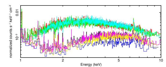
Figure 1.— First-order Chandra/HEG spectra of NGC 4151, grouped to require 20 counts per bin. Error bars are omitted for visual clarity. No models have been applied to the data, but the instrumental effecitive area function (ancillary response file, or ARF) has been removed. The spectra can be placed into two broad categories: those that have a higher flux and/or lower obscuration, and those that have a lower flux and/or higher obscuration. Observation identification numbers (ObsIDs) 0335 (black), 7829 (blue), 16089 (magenta), and 16090 (yellow) have a lower intrinsic flux and/or higher obscuration. ObsIDs 3480 (red), 3052 (green), and 7830 (cyan) have a higher intrinsic flux and/or less obscuration).

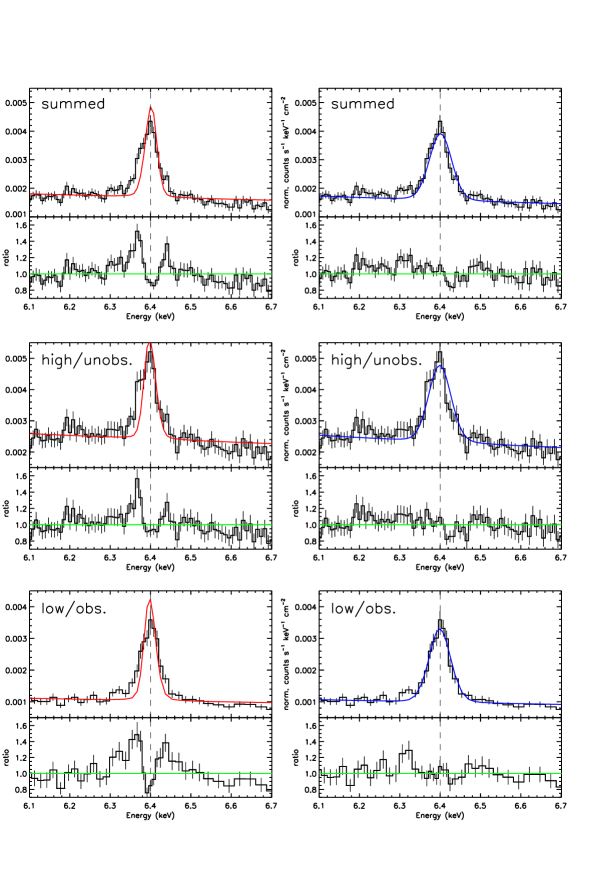
Figure 2.— First-order Chandra/HEG spectra of NGC 4151 in the Fe K band. The spectra have been shifted to the host frame. The top, middle, and bottom rows show spectra from the summed spectrum, “high/unobscured” phase, and “low/obscured” phase, grouped to 20, 20, and 100 counts per bin, respectively. The lefthand column shows fits with a simple Gaussian function with only instrumental broadening. The righthand column shows fits with a Gaussian function with a variable width, $\sigma$. In all cases, the energy of the Gaussian was fixed at $E=6.40$ keV, the laboratory energy for Fe K$\alpha$. These fits show that the line is clearly asymmetric, likely due to a combination of weak Doppler shifts and gravitational red-shifts, and scattering. The results of these and other spectral fits are given in Tables 2 and 3.

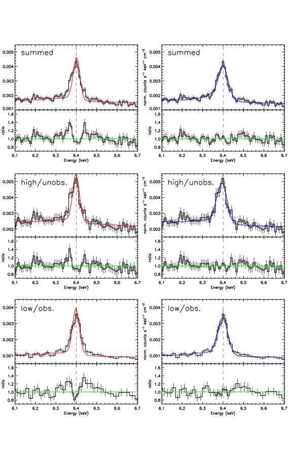
Figure 3.— Fits to the Fe K$\alpha$ line with “mytorus” functions (see, e.g., Murphy & Yaqoob 2009). This function includes scattering effects in dense media that could potentially mimic dynamical broadening. A subtle drop in the model at 6.25 keV, for instance, is the result of 150 eV energy loss from complete 180-degree Compton scattering. Again, the top, middle, and bottom rows show spectra from the summed spectrum, “high/unobscured” phase, and “low/obscured” phase, grouped to 20, 20, and 100 counts per bin, respectively. The lefthand column shows simple fits with “mytorus” model. The righthand column shows fits with the “rdblur” convolution function acting on “mytorus” to account for dynamics. These fits are superior and demonstrate that dynamical broadening is likely required to describe the data. The results of these and other spectral fits are given in Tables 2 and 3.

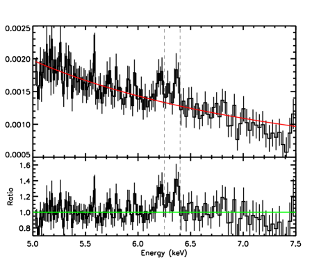
Figure 4.— The difference spectrum of NGC 4151, between the “high/unobscured” and “low/obscured” states. The spectrum was created by subtracting the combined “low/obscured” spectrum from the “high/unobscured” spectrum in units of count rate. The remaining spectrum represents the variable flux between the two states. The data were fit with a simple power-law model after grouping to require 20 counts per bin. Dashed vertical lines at 6.40 keV and 6.25 keV mark the energy at which emission features are expected from neutral Fe K$\alpha$, and the 150 eV energy loss incurred from 180-degree Compton scattering. Emission lines are instead evident to the red of these energies, providing model-independent evidence that the red wing of the narrow Fe K$\alpha$ line in NGC 4151 is stronger in the “high/unobscured” state. When fit with simple Gaussian functions, the features at 6.37 keV and 6.20 keV are significant at the 4$\sigma$ and 5$\sigma$ level of confidence, respectively. Please see the text for additional details.

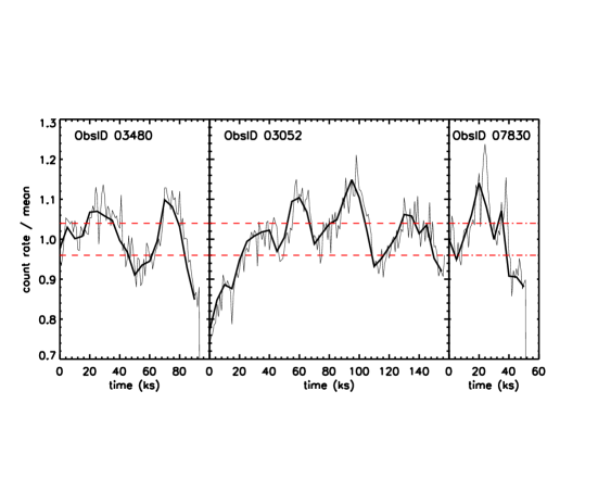
Figure 5.— The light curve of the observations obtained in the “high/unobscured” phase, wherein the Fe K$\alpha$ emission line asymmetry is more pronounced and models measure smaller radii (see Tables 2 and 3). The thick black curve has time bins of 5 ks; the thin gray line has time bins of 1 ks. The count rates are plotted as a ratio to the mean count rate in each observation (the mean rates are nearly identical between observations), to illustrate the relative magnitudes of the variations. The red dashed lines mark flux levels $\pm 4$% above and below the mean in each observation. To explore potential short time scale variations in the narrow Fe K$\alpha$ line, spectra were extracted from intervals that differed by more than 4% from the mean.

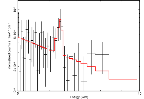
Figure 6.— The difference spectrum of NGC 4151 in the “high/unobscured” state, based on the count rate selections shown in Figure 5. To create this spectrum, the spectrum of the low flux intervals was subtracted from the high flux intervals. Prior to fitting, the data were then grouped to require 50 counts per bin (further binning was done for visual clarity only). The resulting difference spectrum is the variable flux spectrum. The narrow Fe K$\alpha$ line is weakly evident in the difference spectrum, suggesting that it may vary on the time scales typical of the flux intervals. Here, the difference spectrum has been fit with a power-law continuum and a “diskline” model with an inner radius frozen at $R_{in}=130~{}GM/c^{2}$. Dividing the line flux by its minus-side error gives a significance of $3\sigma$.

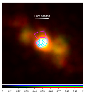
Figure 7.— A “true-color” image of NGC 4151 from a Chandra imaging observation (ObsID 9217). The observation was filtered to create sub-pixels of 0.0492 arc seconds, and further filtered to only include “grade=0” events in order to limit pile-up distortions (Miller et al. 2017). Separate images were made in the 6.3-6.5 keV band (Fe K, shown in blue), 0.8-1.1 keV band (Ne IX-X, shown in green), and 0.5-0.8 keV (O VII-VIII, shown in red). A magenta region marks the location of the Chandra PSF artifact. Cyan contours show that the Fe K region is largely contained within a radius of approximately 0.4 arc seconds, and is consistent with a point source. In contrast, the soft X-ray emission from He-like and H-like charge states is extended and consistent with the optical NLR, as per Wang et al. (2011). The narrow Fe K$\alpha$ line is nuclear, and does not arise in the extended NLR.

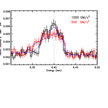
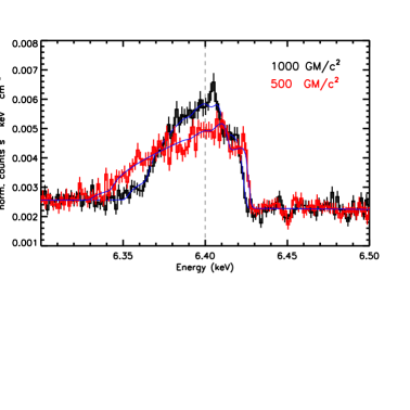
Figure 8.— Simulated 20 ks XARM (left) and ATHENA (right) spectra of NGC 4151. The spectra are binned for visal clarity and shifted to the frame of the host. The simulations were based on the best-fit blurred “mytorus” models for in Table 2. Emission originating from $R\geq 500~{}GM/c^{2}$ (red) and $R\geq 1000~{}GM/c^{2}$ (black) was simulated for both missions. The spectra illustrate the power of calorimeter resolution to easily distinguish even large radii through subtle changes to weak Doppler boosting in Keplerian orbits. Calorimeter spectrometers may enable reverberation mapping from warps at intermediate disk radii and/or the BLR.

References

- (1)
- (2) Antonucci, R., 1993, ARA&A, 31, 473
- (3)
- (4) Arnaud, K., 1996, Astronomical Data Analysis Software and Systems V, ASP Converence Series, eds. G. H. Jacoby and J. Barnes, 101, 17
- (5)
- (6) Bambynek, W., Crasemann, B., Fink, R., Freund, HJ., Mark, H., Swift, C., Price, R., Rao, P., 1972, Rev. Mod. Phys., 44, 716
- (7)
- (8) Barret, D., Lam Trong, T., den Herder, J.-W., et al., 2018, SPIE, subm.
- (9)
- (10) Bentz, M. C., Denney, K. D., Cackett, E. M., et al., 2006, ApJ, 651, 775
- (11)
- (12) Bentz, M. C., Denney, K., Grier, C., et al., 2013, ApJ, 767, 149
- (13)
- (14) Bentz, M. C., & Katz, S., 2015, PASP, 127, 67
- (15)
- (16) Beuchert, T. Markowitz, A., Dauser, T., Garcia, J., Keck, M., Wilms, J., Kadler, M., Brenneman, L., Zdziarski, A., 2017, A&A, 603, 50
- (17)
- (18) Brenneman, L., & Reynolds, C. S., 2006, ApJ, 652, 1028
- (19)
- (20) Cackett, E. M., Zoghbi, A., Reynolds, C., et al., 2014, MNRAS, 438, 2980
- (21)
- (22) Chakrabarti, S., & Wiita, P. J., 1993, ApJ, 411, 602
- (23)
- (24) Chakrabarti, S., & Wiita, P. J., 1994, ApJ, 434, 518
- (25)
- (26) Collin-Souffrin, S., Dyson, J., McDowell, J., Perry, J., 1988, MNRAS, 232, 539
- (27)
- (28) Costantini, E., Kaastra, J., Arav, N., et al., 2007, A&A, 461, 121
- (29)
- (30) Costantini, E., Kaastra, J., Korista, K., Ebrero, J., Arav, N., Kriss, G., Steenbrugge, K., 2010, A&A, 512, 25
- (31)
- (32) Couto, J. D., Kraemer, S. B., Turner, T. J., Crenshaw, D. M., 2016, ApJ, 833, 191
- (33)
- (34) Crenshaw, M., Fischer, T., Kraemer, S., Schmitt, H., 2015, ApJ, 799, 83
- (35)
- (36) Czerny, B., Du, P., Wang., J., Karas, V., 2016, ApJ, 832, 15
- (37)
- (38) Czerny, B., & Hryniewicz, K., 2011, A&A, 525, L8
- (39)
- (40) Czerny, B., Modzelewska, J., Petrogalli, F., Pych, W., Adhikari, T., Zycki, P., Hryniewicz, K., Krupa, M., Swieton, A., Nikolajuk, M., 2015, AdSpR, 55, 1806
- (41)
- (42) Das, V., Crenshaw, D. M., Hutchings, J. B., Deo, R. P., Kraemer, S. B., Gull, T. R., Kaiser, M. E., Nelson, C. H., Wiestrop, D., 2005, AJ, 130, 945
- (43)
- (44) Dauser, T., Garcia, J., wilms, J., Bock, M., Brenneman, L. W., Falanga, M., Fukumura, K., Reynolds, C. S., 2013, MNRAS, 430, 1694
- (45)
- (46) Detmers, R., Kaastra, J., Steenbrugge, K., et al., 2011, A&A, 534, 38
- (47)
- (48) Edelson, R., Gelbord, J., Cackett, E., et al., 2017, ApJ, 840, 41
- (49)
- (50) Elvis, M., Risaliti, G., Nicastro, F., Miller, J. M., Fiore, F., Puccetti, S., 2004, ApJ, 615, L25
- (51)
- (52) Eracleous, M., & Halpern, J., 2003, ApJ, 599, 886
- (53)
- (54) Fabian, A. C., Rees, M. J., Stella, L., White, N., 1989, MNRAS, 238, 729
- (55)
- (56) Fabian, A., Lohfink, A., Kara, E., Parker, M., Vasudevan, R., Reynolds, C., 2015, MNRAS, 451, 4375
- (57)
- (58) Garcia, J., Dauser, T., Reynolds, C. S., Kallman, T., McClintock, J., Narayan, R., Wilms, J., Eikmann, W., 2013, ApJ, 768, 146
- (59)
- (60) Gaskell, C. M., & Sparke, L. S., 1986, ApJ, 305, 175
- (61)
- (62) Georgakakis, A., Salvato, M., Liu, Z., et al., 2017, MNRAS, 469, 3232
- (63)
- (64) Gierlinksi, M., Middleton, M., Ward, M., Done, C., 2008, Nature, 455, 369
- (65)
- (66) Gultekin, K., Richstone, D., Gebhardt, K., et al., 2009, ApJ, 698, 198
- (67)
- (68) Haardt, F., & Maraschi, L., 1993, ApJ, 413, 507
- (69)
- (70) Honig, S. F., Watson, D., Kishimoto, M., Hjorth, J., 2014, Nature, 515, 528
- (71)
- (72) Kaastra, J., Kriss, G. A., Cappi, M., et al., 2014, Science, 345, 64
- (73)
- (74) Kaastra, J., Mehdipour, M., Behar, E., et al., 2018, A&A, subm., arxiv:1805.03538
- (75)
- (76) Keck, M. L., Brenneman, L. W., Ballantyne, R. R., et al., 2015, ApJ, 806, 149
- (77)
- (78) Kollatschny, W., 2003, A&A, 407, 461
- (79)
- (80) Liu, J., 2016, MNRAS, 463, 108
- (81)
- (82) Maloney, P., Begelman, M., Pringle, J., 1996, ApJ, 472, 582
- (83)
- (84) Mehdipour, M., Kaastra, J., Kriss, G., et al., 2017, A&A, 607, 28
- (85)
- (86) Miller, J. M., 2007, ARA&A, 45, 441
- (87)
- (88) Miller, J. M., Bautz, & McNamara, B., 2017, ApJ, 850, L3
- (89)
- (90) Miller, J. M., Fabian, A. C., Kaastra, J., Kallman, T., King, A. L., Proga, D., Raymond, J., Reynolds C. S., 2015, ApJ, 814, 87
- (91)
- (92) Miller, J. M., Raymond, J., Fabian, A. C., Gallo, E., Kaastra, J., Kallman, T., King, A. L., Proga, D., Reynolds, C. S., Zoghbi, A., 2016, ApJ, 821, L9
- (93)
- (94) Moran, J., Greenhill, L., Herrnstein, J., Diamond, P., Miyoshi, M., Nakai, N., Inque, M., 1995, PNAS, 9211427
- (95)
- (96) Murphy, K. K., & Yaqoob, T., 2009, MNRAS, 397, 1549
- (97)
- (98) Nandra, K., Barret, D., Barcons, X., et al., 2013, White Paper submitted to the ESA call for L2 and L3 science programs, arxiv:1306.3207
- (99)
- (100) Nandra, K, O’Neill, P. M., George, I. M., Reeves, J. N., 2007, MNRAS, 382, 194
- (101)
- (102) Nguyen, K., & Bogdanovic, T., 2016, ApJ, 828, 68
- (103)
- (104) Reis, R., Miller, J. M., Reynolds, M., Gultekin, K., Maitra, D., King, A., Strohmayer, T., 2012, Science, 337, 949
- (105)
- (106) Reynolds, C., & Nowak, M., 2003, Physics Reports, 377, 389
- (107)
- (108) Reynolds, C., Ueda, Y., Awaki, H., et al., Astro-H White Paper - AGN Reflection, arxiv:1412.1177
- (109)
- (110) Shu, X. W., Yaqoob, T., Wang, J. X., 2010, ApJS, 187, 581
- (111)
- (112) Ulvestad, J. S., Wong, D. S., Taylor, G. B., Gallimore, J. F., Mundell, C. G., 2005, ApJ, 130, 936
- (113)
- (114) Urry, C. M., & Padovani, P., 1995, PASP, 107, 308
- (115)
- (116) Urry, M., 2003, in “Active Galactic Nuclei: From Central Engine to Host Galaxy”, eds F. Combes, I. Shlosman, vol 290 of “Astronomical Society of the Pacific Conference Series”
- (117)
- (118) Vaughan, S., & Fabian, A. C., 2004, MNRAS, 348, 1415
- (119)
- (120) Wang, J., Fabbiano, G., Elvis, M., Risaliti, G., Karovska, M., Zezas, A., Mundell, C. G., Dumas, G., Schinnerer, E., 2011, ApJ, 742, 23
- (121)
- (122) Yaqoob, T., & Murphy, K., 2010, MNRAS, 412, 277
- (123)
- (124) Zoghbi, A., Fabian, A. C., Reynolds, C. S., Cackett, E. M., 2012, MNRAS, 422, 129
- (125)