Learning Timed Automata
via Genetic Programming

Abstract

Model learning has gained increasing interest in recent years. It derives behavioural models from test data of black-box systems. The main advantage offered by such techniques is that they enable model-based analysis without access to the internals of a system. Applications range from fully automated testing over model checking to system understanding. Current work focuses on learning variations of finite state machines. However, most techniques consider discrete time. In this paper, we present a method for learning timed automata, finite state machines extended with real-valued clocks. The learning method generates a model consistent with a set of timed traces collected by testing. This generation is based on genetic programming, a search-based technique for automatic program creation. We evaluate our approach on $\mathbf{44}$ timed systems, comprising four systems from the literature and $\mathbf{40}$ randomly generated examples.

I Introduction

Test-based model-learning techniques have gained increasing interest in recent years. Basically, these techniques derive formal system models from (test) observations. They therefore enable model-based reasoning about software systems while requiring only limited knowledge about the system at hand. Put differently, such techniques allow for model-based verification of black-box systems if they are amenable to testing.

Peled et al. [44] performed pioneering work in this area by introducing Black Box Checking, automata-based model checking for black-box systems. It involves interleaved model learning, model checking and conformance testing and built the basis for various follow-up work [25, 18]. More recent work in this area includes for example model checking of network protocols [19, 20], and differential testing on the model level [45, 10, 48]. The basic framework we target is shown in Fig. 1. In the simplest case, we interact with a system by testing, learn a model from system traces and then perform some kind of verification. However, feedback loops are possible: we can derive additional tests from the preliminary learned model, and we could use counterexample traces from model checking as tests.

Figure 1: General framework for test-based learning enabling verification.

Learning-based verification has great potential, but applications often use modelling formalisms with low expressiveness such as Mealy machines. This can be attributed to the availability of efficient implementations of learning algorithms for variations of finite automata, e.g. in LearnLib [30], and comparably low support for richer automata types; especially timed systems have received little attention. Notable works include learning of real-time automata and a probabilistic variant thereof [50, 51] by Verwer et al. and techniques for learning event-recording automata described by Grinchtein et al. [23, 24]. Recently, Jonsson and Vaandrager also developed an active learning technique for Mealy machines with timers [32]. Our goal is to overcome limitations of these approaches. Real-time automata, e.g., are restricted in their expressiveness and learning of event-recording automata has a high runtime complexity.

Scope and Outline

In this work, we focus on the learning part in Fig. 1. Generally, model learning may be performed either passively or actively [15]. In the former, preexisting data, such as system logs or existing test data, serves as a basis, while in the latter, the system is actively queried during the testing phase, i.e. tested, to gain relevant information. The technique we propose is passive in general, but active extensions are possible.

More specifically, we use a form of genetic programming [34] to automatically learn a deterministic timed automaton (TA) consistent with a given set of test cases. Our main contribution is the development of a genetic-programming framework for TA which includes mutation operators, a crossover procedure, and a corresponding, fine-grained fitness-evaluation. We evaluate this approach, a meta-heuristic search, on four manually created TA and several randomly generated TA. The evaluation demonstrates that the search reliably converges to a TA consistent with the test cases given as training data. Furthermore, we simulate each generated TA on independently produced test data to show that our identified solutions generalise well, thus do not overfit to training data.

This paper is structured as follows. The next section contains background information on TA and genetic programming. Section III describes our approach to learning TA. Applications of this approach are presented in Sect. IV. In Sect. V, we provide a summary and discuss related work, as well as potential extensions.

II Preliminaries

II-A Timed Automata

Timed automata are finite automata enriched with real-valued variables called clocks [9]. Clocks measure the progress of time which elapses while an automaton resides in some location. Transitions can be constrained based on clock values and clocks may be reset upon the execution of transitions. We denote the set of clocks by $\mathcal{C}$ and the set of guards over $\mathcal{C}$ by $\mathcal{G}(\mathcal{C})$. Guards are conjunctions of constraints of the form $c\oplus k$, with $c\in\mathcal{C},\oplus\in\{>,\geq,\leq,<\},k\in\mathbb{N}$. Transitions are labelled by input and output actions, denoted by $\Sigma_{I}$ and $\Sigma_{O}$ respectively, with $\Sigma=\Sigma_{I}\cup\Sigma_{O}$. Input action labels are suffixed by $?$, while output labels contain the suffix $!$. A timed automaton over $(\mathcal{C},\Sigma)$ is a triple $\langle L,l_{0},E\rangle$, where $L$ is a finite non-empty set of locations, $l_{0}\in L$ is the initial location and $E$ is the set of edges, with $E\subseteq L\times\Sigma\times\mathcal{G}(\mathcal{C})\times 2^{\mathcal{C}}\times L$. We write $l\xrightarrow{g,a,r}l^{\prime}$ for an edge $(l,g,a,r,l^{\prime})\in E$ with a guard $g$, an action label $a$, and clock resets $r$.

Example II.1 (Train TA Model).

Figure 2 shows a TA model of a train, for which we have $\Sigma_{I}=\{\mathit{start}?,\mathit{stop}?,\mathit{go}?\}$, $\Sigma_{O}=\{\mathit{appr}!,\mathit{enter}!,\mathit{leave}!\}$, $\mathcal{C}=\{c\}$, $L=\{l_{0},\ldots,l_{5}\}$, and $E=\{l_{0}\xrightarrow{\top,\mathit{start}?,\{c\}}l_{1},\ldots\}$. From initial location $l_{0}$, the train accepts the input $\mathit{start}?$, resetting clock $c$. After that, it can produce the output $\mathit{appr}!$ if $c\geq 5$, i.e the train may approach $5$ time units after it is started.

Figure 2: Train TA.

The semantics of a TA is given by a timed transition system (TTS) $\langle Q,q_{0},\Sigma,T\rangle$, with states $Q=L\times{\mathbb{R}_{\geq 0}}^{\mathcal{C}}$, initial state $q_{0}$, and transitions $T\subseteq Q\times(\Sigma\cup\mathbb{R}_{\geq 0})\times Q$, for which we write $q~{}\xrightarrow{e}~{}q^{\prime}$ for $(q,e,q^{\prime})\in T$. A state $q=(l,\nu)$ is a pair consisting of a location $l$ and a clock valuation $\nu$. For $r\subseteq\mathcal{C}$, we denote resets of clocks in $r$ by $\nu[r]$, i.e. $\forall c\in r:\nu[r](c)=0$ and $\forall c\in\mathcal{C}\setminus r:\nu[r](c)=\nu(c)$. Let $(\nu+d)(c)=\nu(c)+d$ for $d\in\mathbb{R}_{\geq 0},c\in\mathcal{C}$ denote the progress of time and $\nu\models\phi$ denote that valuation $\nu$ satisfies formula $\phi$. Finally, $\mathbf{0}$ is the valuation assigning zero to all clocks and the initial state $q_{0}$ is $(l_{0},\mathbf{0})$. Transitions of TTSs are either delay transitions $(l,\nu)\xrightarrow{d}(l,\nu+d)$ for a delay $d\in\mathbb{R}_{\geq 0}$, or discrete transitions $(l,\nu)\xrightarrow{a}(l^{\prime},\nu[r])$ for an edge $l\xrightarrow{g,a,r}l^{\prime}$ such that $\nu\models g$. Delays are usually further constrained, e.g. by invariants [27] limiting the sojourn time in locations.

Timed Traces. We use the terms timed traces and test sequences similarly to [46]. The latter are sequences of inputs and corresponding execution times, while the former are sequences of inputs and outputs, together with their times of occurrence (produced in response to a test sequence). A test sequence $\mathit{ts}$ is an alternating sequence of non-decreasing time stamps $t_{j}$ and inputs $i_{j}$, i.e. $\mathit{ts}=t_{1}\cdot i_{1}\cdots t_{n}\cdot i_{n}\in(\mathbb{R}_{\geq 0}\times\Sigma_{I})^{*}$ with $\forall j\in\{1,\ldots,n-1\}:t_{j}\leq t_{j+1}$. Informally, a test sequence prescribes that $i_{j}$ should be executed at time $t_{j}$. A timed trace $\mathit{tt}\in(\mathbb{R}_{\geq 0}\times\Sigma)^{*}$ consists of inputs interleaved with outputs produced by a timed system. Analogously to test sequences, its timestamps are non-decreasing.

II-A1 Assumptions on Timed Systems

Testing based on TA often places further assumptions on TA [46, 27]. Since we learn models from tests we make similar assumptions (closely following [27]). We describe these assumptions on the level of semantics and use $q\xrightarrow{a}$ to denote $\exists q^{\prime}:q\xrightarrow{a}q^{\prime}$ and $q\centernot{\xrightarrow{a}}$ for $\nexists q^{\prime}:q\xrightarrow{a}q^{\prime}$:

1. Determinism. A TA is deterministic iff for every state $s=(l,\nu)$ and every action $a\in\Sigma$, whenever $s\xrightarrow{a}s^{\prime}$, and $s\xrightarrow{a}s^{\prime\prime}$ then $s^{\prime}=s^{\prime\prime}$.

2. Input Enabledness. A TA is input enabled iff for every state $s=(l,\nu)$ and every input $i\in\Sigma_{I}$, we have $s\xrightarrow{i}$.

3. Output Urgency. A TA shows output-urgent behaviour if outputs occur immediately as soon as they are enabled, i.e. for $o\in\Sigma_{O}$, if $s\xrightarrow{o}$ then $s\centernot{\xrightarrow{d}}$ for all $d\in\mathbb{R}_{\geq 0}$. I.e., outputs must not be delayed.

4. Isolated Outputs. A TA has isolated outputs iff whenever an output may be executed, then no other output is enabled, i.e. if $\forall o\in\Sigma_{O},\forall o^{\prime}\in\Sigma_{O}$ $q\xrightarrow{o}$ and $q\xrightarrow{o^{\prime}}$ implies $o=o^{\prime}$.

It is necessary to place restrictions on the sojourn time in locations to establish output urgency. Deadlines provide a simple way to model the assumption that systems are output urgent [14]. With deadlines it is possible to model eager actions. We use this concept and implicitly assume all learned output edges to be eager. This means that outputs must be produced as soon as their guards are satisfied. For that, we extend the semantics given above by adding the following restriction: delays $(l,\nu)\xrightarrow{d}(l^{\prime},\nu+d)$ are only possible if $\forall~{}d^{\prime}~{}\in~{}\mathbb{R}_{\geq 0},d^{\prime}<d:\nu+d^{\prime}\models\lnot\bigvee_{g\in G_{O}}g$, where $G_{O}=\{g|\exists l^{\prime},a,r:l\xrightarrow{g,a,r}~{}l^{\prime},a\in\Sigma_{O}\}$ are the guards of outputs in location $l$. To avoid issues related to the exact time at which outputs should be produced, we further restrict the syntax of TA by disallowing strict lower bounds for output edges. Uppaal [36] uses invariants rather than deadlines to limit sojourn time. In order to analyse TA using Uppaal, we use the translation given in [22]. We implicitly add self-loops to all states $s=(l,\nu)$ for inputs $i$ undefined in $s$, i.e. we add $(l,\nu)\xrightarrow{i}(l,\nu)$ if $\nu\cancel{\models}\bigvee_{\exists l^{\prime},r:l\xrightarrow{g,i,r}l^{\prime}}g$. This ensures input enabledness while avoiding TA cluttered with input self-loops.

The assumptions placed on systems under test ensure testability [27]. Assuming that SUTs can be modelled in some modelling formalism is usually referred to as testing hypothesis. Placing the same assumptions on learned models simplifies checking conformance between model and SUT. The execution of a test sequence on such a model uniquely determines a response [46], and due to input-enabledness we may execute any test sequence. This allows us to use equivalence as conformance relation between learned models and SUT. What is more, we can approximate checking equivalence between the learned models and the SUT by executing test sequences on the models and check for equivalence between the SUT’s responses and the response predicted by the models.

II-B Genetic Programming

Genetic programming [34] is a search-based technique to automatically generate programs exhibiting some desired behaviour. Like Genetic Algorithms [41], it is inspired by nature. Programs, also called individuals, are iteratively refined by: (1) fitness-based selection followed by (2) operations altering program structure, like mutation and crossover. Fitness measures are problem-specific and may for instance be based on tests. In this case, one could assign a fitness value proportional to the number of tests passed by an individual. The following basic functioning principle underlies genetic programming.

1. Randomly create an initial population.

2. Evaluate the fitness of each individual in the population.

3. If an acceptable solution has been found or the maximum number of iterations has been performed: stop and output the best individual

4. Otherwise select an individual based on its fitness and apply one of:

   Mutation:

   change a part of the individual creating a new individual.

   Crossover:

   select another individual according to its fitness and combine both individuals to create offspring.

   Reproduction:

   copy the individual to create a new equivalent individual.

5. Form a new population from the newly created individuals and go to Step 2.

Several variations of and additions to this general approach exist and, in the following, we are going to discuss additional details that we will apply in Sect. III.

Mutation Strength and Parameter Adaptation. In meta-heuristic search techniques, like evolution strategies [12], mutation strength typically describes the level of change caused by mutations. This parameter heavily influences search and therefore there exist various schemes to adapt it. Since the optimal value for it is problem-specific, it makes sense to evolve throughout the search together with the actual individuals. Put differently, individuals are equipped with their own mutation strength, which is mutated during the search. Individuals with good mutation strength are assumed to survive selection and reproduce.

Elitism. Elitist strategies keep track of a portion of the fittest individuals found so far and copy them into the next generation [41]. This may improve performance, as correctly identified partial solutions cannot be forgotten.

Subpopulations and Migration. Due to their nature, genetic algorithms and genetic programming lend themselves to parallelisation. Several populations may, e.g., be evolved in parallel, which is particularly useful if speciation is applied [42]. In speciation, different subpopulations explore different parts of the search space. In order to exchange information between the subpopulations, it is common that individuals migrate between them.

III Genetic Programming for Timed Automata

Figure 3: Overview of genetic programming.

Figure 4: Creating a new global population.

We introduced genetic programming above and discuss our implementation in the following. Figure 3 provides an overview of the steps we perform, while Figure 4 shows the creation of a new population in more detail.

We start with testing of the SUT. For that, we generate $n_{\mathrm{test}}$ test sequences and execute them, to collect $n_{\mathrm{test}}$ timed traces. Our goal is then to genetically program a TA consistent with the collected timed traces. Put differently, we want to generate a TA that produces the same outputs as the SUT in response to the inputs of the test sequences. For the following discussion, we say that a TA passes a timed trace $t$ if it produces the same outputs as the SUT when simulating the test sequence corresponding to $t$. Otherwise it fails $t$.

Generally, we evolve two populations of TA simultaneously, a global population which is evaluated on all the traces and a local population which is only evaluated on the traces that fail on the fittest automaton of the global population. Both are initially created in the same way and contain $n_{\mathrm{pop}}$ TA. After initial creation, the global population is evaluated on all $n_{\mathrm{test}}$ traces. During that, we basically test the TA and check how many traces each TA passes and assign fitness values accordingly, i.e., the more passing traces the fitter. Additionally, we add a fitness penalty for model size. The local population is evaluated only on a subset $\mathcal{T}_{\mathrm{fail}}$ of the traces. This subset $\mathcal{T}_{\mathrm{fail}}$ contains all traces which the fittest TA fails, and which likely most of the other TA fail as well. With the local population, we are able to explore new parts of the search space more easily since we may ignore functionality already modelled by the global population. We integrate functionality found via this local search into the global population through migration and migration combined with crossover. To avoid overfitting to a low number of traces, we ensure that $\mathcal{T}_{\mathrm{fail}}$ contains at least $\frac{n_{\mathrm{test}}}{100}$ traces. If there are less actually failing traces, we add randomly chosen traces from all $n_{\mathrm{test}}$ traces to $\mathcal{T}_{\mathrm{fail}}$.

After evaluation, we stop if we either reached the maximum number of generations $g_{\mathrm{max}}$, or the fittest TA passes all traces and has not changed in $g_{\mathrm{change}}$ generations. Note that two TA passing all traces may have different fitness values depending on model size, i.e. $g_{\mathrm{change}}$ controls how long we try to decrease the size of the fittest TA. The rationale behind this is that TA of smaller size are less complex and therefore simpler to comprehend.

If not stopped, we create new populations of TA, which works slightly differently for the local and the global population. Figure 4 illustrates the creation of a new global population. Before creating new TA, existing TA may migrate from the local to the global population. For that, we check each of the fittest $n_{\mathrm{mig}}$ local TA and add it to the global population if it passes at least one trace from $\mathcal{T}_{\mathrm{fail}}$. We generally set $n_{\mathrm{mig}}$ to $\frac{5n_{\mathrm{pop}}}{100}$, i.e. the top five per cent of the local population are allowed to migrate. After migration, we create $n_{\mathrm{pop}}$ new TA through the application of one of three operations:

• with probability $1-p_{\mathrm{cr}}$: select a TA from the global population and mutate it

• with probability $\frac{p_{\mathrm{cr}}}{2}$: select two TA from the global population and perform crossover with these

• with probability $\frac{p_{\mathrm{cr}}}{2}$: select one TA from each population and perform crossover with these

The rationale behind migration combined with crossover is that migrated TA may have low fitness from a global point of view and will therefore not survive selection. They may, however, have desirable features which can be transferred via crossover. For the local population, we perform the same steps, but without any migration, in order to keep the local search independent. Once we have new populations, we start a new generation by evaluating the new TA.

A detail not illustrated in Fig. 3 is our implementation of elitism. We always keep track of the fittest TA found so far for both populations. In each generation, we add these fit TA to their respective populations after mutation.

Parameters. Our implementation could be controlled by a large number of parameters. To ease applicability and to avoid the need for meta-optimisation of parameter settings for a particular SUT, we fixed as many as possible to constant values. The actual values, like $\frac{5n_{\mathrm{pop}}}{100}$ for $n_{\mathrm{mig}}$, are motivated by experiments. The remaining user-specifiable parameters can usually be set to default values or chosen based on guidelines. For instance, $n_{\mathrm{pop}}$, $g_{\mathrm{max}}$, and $n_{\mathrm{test}}$ may be chosen as large as possible, given available memory and maximum computation time.

III-A Creation of Initial Random Population

TABLE I: Parameters for Initial Creation of TA

Name	Short description
$\Sigma_{I}$ & $\Sigma_{O}$	the input and output action labels on edges
$n_{\mathrm{clock}}$	number of clocks in the set of clocks $\mathcal{C}$
$c_{\mathrm{max}}$	approximate largest constant in clock constraints

As discussed, we initially create $n_{\mathrm{pop}}$ random TA. The parameters in Table I control this creation. Note, $c_{\mathrm{max}}$ is an approximation, because mutations may increase constants. Each TA has initially only two locations, as we intend to increase size and thereby complexity only through mutation and crossover. Moreover, it is assigned the given action labels and has a set of $n_{\mathrm{clock}}$ clocks. During creation, we add random edges, such that at least one edge connects the initial location to the other location.

We create edges entirely randomly, whereby the number of constraints in guards as well as the number of clock resets are geometrically distributed with fixed parameters. The label of an edge, the relational operators and constants in constraints are chosen uniformly at random from the respective sets $\Sigma$, $\{<,\leq,\geq,>\}$, and $[0\mathinner{\ldotp\ldotp}c_{\mathrm{max}}]$ (operators for outputs exclude $>$). The source and target locations are also chosen uniformly at random from the set of locations, i.e. initially we choose from two locations.

If the required number of clocks is not known a priori, we suggest setting $n_{\mathrm{clock}}=1$ and increasing it only if it is not possible to find a valid TA. A similar approach could be used for $c_{\mathrm{max}}$, i.e. setting it to a low value for an initial search.

III-B Fitness Evaluation

III-B1 Simulation

We simulate the TA to evaluate their fitness. In the beginning of this section, we discussed failing and passing trace, but evaluation is more fine grained. We execute the inputs of each timed trace and observe produced outputs until (1) the simulation is complete, (2) an expected output is not observed, or (3) output isolation is violated (output non-determinism).

In general, if $\mathcal{T}$ is a deterministic, input-enabled TA with isolated and urgent outputs and $\mathit{ts}$ is a test sequence, then executing $\mathit{ts}$ on $\mathcal{T}$ uniquely determines a timed trace $\mathit{tt}$. By the testing hypothesis, the SUT fulfils these assumptions. However, TA generated through mutation and crossover are input-enabled, but may show non-deterministic behaviour. Hence, simulating a test sequence or a timed trace on a generated TA may follow multiple paths of states. Some of these paths may produce the expected outputs and some may not. Our goal is to find a TA that is both correct, i.e. produces the same outputs as the SUT, and is deterministic. Consequently, we reward these properties with positive fitness.

The simulation function $\textsc{sim}(\mathcal{G},\mathit{tt})$, simulates a timed trace $\mathit{tt}$ on a generated TA $\mathcal{G}$ and returns a set of timed traces. It uses the TTS semantics for TA but does not treat outputs as urgent outputs. From the initial state $(l_{0},\mathbf{0})$, where $l_{0}$ is the initial location of $\mathcal{G}$, it performs the following steps for each $t_{i}e_{i}\in\mathit{tt}$ with $t_{0}=0$:

1. From state $q=(l,\nu)$

2. Delay for $d=t_{i}-t_{i-1}$ to reach $q^{d}=(l,\nu+d)$

3. If $e_{i}\in\Sigma_{I}$, i.e. it is an input:

   1. If $\exists o\in\Sigma_{O},d^{o}\leq d:(l,\nu+d^{o})\xrightarrow{o}$, i.e. an output would have been possible while delaying or at time $t_{i}$

   2. then mark $e_{i}$

   3. If $\exists q^{1},q^{2},q^{1}\neq q^{2}:q^{d}\xrightarrow{e_{i}}q^{1}\land q^{d}\xrightarrow{e_{i}}q^{2}$

   4. then mark $e_{i}$

   5. For all $q^{\prime}$ such that $q^{d}\xrightarrow{e_{i}}q^{\prime}$

   6. carry on exploration with $q^{\prime}$

4. If $e_{i}\in\Sigma_{O}$, i.e. it is an output:

   1. If $\exists o\in\Sigma_{O},d^{o}<d:(l,\nu+d^{o})\xrightarrow{o}$, i.e. an output would have been possible while delaying

   2. stop exploration

   3. If $\exists q^{1},q^{2},q^{1}\neq q^{2}:q^{d}\xrightarrow{e_{i}}q^{1}\land q^{d}\xrightarrow{e_{i}}q^{2}$ or $\exists o,o\neq e_{i}:q^{d}\xrightarrow{o}$

   4. stop exploration

   5. If there is a $q^{\prime}$ such that $q^{d}\xrightarrow{e_{i}}q^{\prime}$

   6. carry on exploration with $q^{\prime}$

The procedure shown above allows for two types of non-determinism. During delays before executing an input, we may ignore outputs (3.1.) and we may explore multiple paths with inputs (3.3.). We mark these inputs to be non-deterministic, through (3.1. and 3.2.). Since we explore multiple paths, a single input $e_{i}$ may be marked along one path but not marked along another path. In contrast, we do not allow for non-determinism with respect to outputs to avoid issues with trivial TA which produce each output all the time. These would completely simulate all traces, but would not be useful.

During exploration, $\textsc{sim}(\mathcal{G},\mathit{tt})$ collects and returns timed traces $tts$, which are basically prefixes of $\mathit{tt}$ but with marked and unmarked inputs. For fitness computation, we defined four auxiliary functions. The first one assigns a simulation verdict, which is $\mathtt{PASS}$ if $\mathcal{G}$ behaves deterministically and produces the expected outputs. It is $\mathtt{NONDET}$ if it produces the correct outputs along at least one execution path, but behaves non-deterministically. Otherwise it is $\mathtt{FAIL}$.

verdict $$(tts)=$$

$$\begin{cases}\mathtt{PASS}&\text{ if }|\mathit{tts}|=1\land\mathit{tt}\in\mathit{tts}\\ \mathtt{NONDET}&\text{ if }|\mathit{tts}|>1\land\exists tt^{\prime}\in\mathit{tts}:|tt^{\prime}|=|tt|\\ \mathtt{FAIL}&\text{ otherwise }\\ \end{cases}$$

Function $\textsc{steps}(\mathit{tts})$ returns the maximum number of unmarked inputs in a trace in $\mathit{tts}$, i.e. the deterministic steps, and $\textsc{out}(\mathit{tts})$ returns the number of outputs along the longest traces in $\mathit{tts}$. Finally, $\textsc{size}(\mathcal{G})$ returns the number of edges.

Note that a TA, which produces a $\mathtt{PASS}$ verdict for all timed traces, behaves equivalently to the SUT for these traces. As indicated at the end of Sect. II-A, we approximate equivalence testing via simulation with sim.

III-B2 Fitness Computation

In order to compute the fitness, we assign the weights $w_{\mathtt{PASS}}$, $w_{\mathtt{NONDET}}$, $w_{\mathtt{FAIL}}$, $w_{\textsc{steps}}$, $w_{\textsc{out}}$, and $w_{\textsc{size}}$ to the gathered information of $\mathcal{G}$. Basically, we give some positive fitness for deterministic steps, correctly produced outputs, and verdicts, but penalise size. Let $\mathcal{TT}$ be the timed traces on which $\mathcal{G}$ is evaluated. The fitness $\textsc{fit}(\mathcal{G})$ with $tts=\ \textsc{sim}(\mathcal{G},tt)$ is then:

$$\textsc{fit}(\mathcal{G})=\ \sum_{tt\in\mathcal{TT}}\textsc{fit}(\mathcal{G},tt)-w_{\textsc{size}}\ \textsc{size}(\mathcal{G})\;\text{ where }$$

$$\textsc{fit}(\mathcal{G},tt)=\ w_{\textsc{verdict}(tts)}+w_{\textsc{steps}}\ \textsc{steps}(tts)$$

$$+w_{\textsc{out}}\ \textsc{out}(tts)$$

Fitness evaluation adds further parameters. We identified guidelines for choosing them adequately. We generally set $w_{\mathtt{FAIL}}=0$ and use $w_{\textsc{out}}$ as basis for other weights. Usually, we set $w_{\textsc{step}}=w_{\textsc{out}}/2$ and $w_{\mathtt{PASS}}=k\cdot l\cdot w_{\textsc{out}}$, where $l$ is the average length of test sequences and $k$ is a small natural number, e.g. $4$. More important than the exact value of $k$ is setting $w_{\mathtt{NONDET}}=w_{\mathtt{PASS}}/2$ which gives positive fitness to correctly produced timed traces but with a bias towards deterministic solutions. The weight $w_{\textsc{size}}$ should be chosen low, such that it does not prevent adding of necessary edges. We usually set it to $w_{\textsc{step}}$. It needs to be non-zero, though. Otherwise an acceptable solution could be a tree-shaped automaton exactly representing $\mathcal{TT}$ without generalisation.

III-C Creation of New Population

We discussed how we create a new population at the beginning of this section on the basis of Fig. 4 and we will now present details of the involved steps.

III-C1 Migration

In the context of migration, we consider non-deterministically passed traces to be failed, i.e. $\mathcal{T}_{\mathrm{fail}}$ contains all traces for which the fittest TA of the global population produces a verdict other than $\mathtt{PASS}$. The rationale behind this is that we want to improve for traces with both $\mathtt{FAIL}$ and $\mathtt{NONDET}$ verdict.

III-C2 Selection

We use the same selection strategy for mutation and crossover, except that crossover must not select the same parent twice. In particular, we combine truncation and probabilistic tournament selection: first, we discard the $(n_{\mathrm{pop}}-n_{\mathrm{sel}})$ worst-performing non-migrated TA (truncation). Then, for each individual selection, we perform a tournament selection from the remaining $n_{\mathrm{sel}}$ TA of the global population and migrated TA. Probabilistic tournament selection [28] randomly chooses a set of $n_{\mathrm{t}}$ TA and orders them by their fitness. It then selects the $i^{th}$ TA with probability $p_{i}$, which we set to $p_{i}=p_{\mathrm{t}}(1-p_{\mathrm{t}})^{i-1}$ for $i\in[1\mathinner{\ldotp\ldotp}n_{\mathrm{t}}-1]$ and $p_{n_{\mathrm{t}}}=(1-p_{\mathrm{t}})^{n_{\mathrm{t}}-1}$, with $n_{\mathrm{t}}=10$ and $p_{\mathrm{t}}=0.5$.

Truncation selection is mainly motivated by the observation that it increases convergence speed during early generations by concentrating on the fittest TA. However, it can be expected to cause a larger loss of diversity than other selection mechanisms [13]. As a result, search may converge to a suboptimal solution, because TA that might need several generations to evolve to an optimal solution are simply discarded through truncation. Therefore, we gradually increase $n_{\mathrm{sel}}$ until it becomes as large as $n_{\mathrm{pop}}$ such that no truncation is applied in later generations. For the same reason, we do not discard migrated TA, since they may possess valuable features.

TABLE II: Mutation Operators

Name	Short description
add constraint	adds a guard constraint to an edge
change guard	select edge and create a random guard if the edge does not have a guard, otherwise mutate a constraint of its guard
change target	changes the target location of an edge
remove guard	remove either all or a single guard constraint from an edge
change resets	remove or add clocks to the clock resets of an edge
remove edge	removes a selected edge
add edge	adds an edge connecting randomly chosen locations
sink location	adds a new location
merge location	merges two locations
split location	splits a location $l$ by creating a new location $l^{\prime}$ and redirecting an edge reaching $l$ to $l^{\prime}$
add location	adds a new location and two edges connecting the new location to existing locations
split edge	replaces an edge $e$ with either the sequence $e^{\prime}\cdot e$ or $e\cdot e^{\prime}$ where $e^{\prime}$ is a new random edge (adds a location to connect $e$ and $e^{\prime}$)

III-C3 Application of Mutation Operators

We implemented mutation operators for changing all aspects of TA, such as adding and removing clock constraints. Table II lists all operators. Whenever an operator selects an edge or a location, the selection is random, but favours locations and edges which are associated with faults and non-deterministic behaviour. We augment TA with such information during fitness evaluation. To create an edge, we create random guards and reset sets, and choose a random label, like for the initial creation of TA.

The mutation operators form three groups separated by bold horizontal lines. The first and largest group contains basic operators, which are sufficient to create all possible automata. The second group is motivated by the basic principle behind automata learning algorithms. Passive algorithms often start with a tree-shaped representation of traces and transform this representation into an automaton via iterated state-merging [15]. Active learning algorithms on the other hand usually start with a low number of locations and add new locations if necessary. This can be interpreted as splitting of existing locations, an intuition which also served as a basis for test-case generation in active automata learning [8]. The last two operators are motivated by observations during experiments: add location increases the automaton size but avoids creating deadlock states, unlike the operator sink location. Split edge addresses issues related to input enabledness, where an input $i$ is implicitly accepted without changing state, although an edge labelled $i$ should change the state. The operator aims to introduce such edges. For mutation, we generally select one of the operators uniformly at random.

III-C4 Simplification

In addition to mutation, we apply a simplification procedure. It changes the syntactic representation of TA without affecting semantics, by, e.g., removing unreachable locations and self-loops for inputs which do not reset clocks. This limits the search to relevant parts of the search space, i.e. we do not mutate unreachable edges. The parameter $g_{\mathrm{simp}}$ specifies the number of generations between executions of simplification. Note that we check only the underlying graph of the TA, but do not consider clock values to ensure fast operation.

1:$(l^{1},l^{2})\leftarrow\text{current product location}$

2:for all $l^{1}\xrightarrow{g^{1},a,r^{1}}{l^{1}}^{\prime}$ do

3:     if $l^{2}\xrightarrow{g^{2},a,r^{2}}{l^{2}}^{\prime}$ then $\triangleright$ synchronise on label $a$

4:         add ($(l^{1},l^{2})\xrightarrow{\textsc{choose}(g^{1},g^{2}),a,\textsc{choose}(r^{1},r^{2})}({l^{1}}^{\prime},{l^{2}}^{\prime})$

5:     else

6:         add ($(l^{1},l^{2})\xrightarrow{g^{1},a,r^{1}}({l^{1}}^{\prime},\textsc{chooseFrom}(L^{2}))$      

7:for all $l^{2}\xrightarrow{g^{2},a,r^{2}}{l^{2}}^{\prime}$ s.t. $\nexists g^{1},r^{1},{l^{1}}^{\prime}:l^{1}\xrightarrow{g^{1},a,r^{1}}{l^{1}}^{\prime}$ do

8:     add ($(l^{1},l^{2})\xrightarrow{g^{2},a,r^{2}}(\textsc{chooseFrom}(L^{1}),{l_{2}}^{\prime})$

Figure 5: Crossover for location $(l^{1},l^{2})$.

III-C5 Crossover

We basically implement crossover as a randomised product of two parents. Briefly, it works as follows. Let $L^{1}$ and $L^{2}$ be the locations of the two parents and let ${l_{0}}^{1}$ and ${l_{0}}^{2}$ be their respective initial locations, then the locations of the offspring are given by $L^{1}\times L^{2}$. Beginning from ${l_{0}}^{1}$ and ${l_{0}}^{2}$ and the initial product location $({l_{0}}^{1},{l_{0}}^{2})$, we explore both parents in a breadth-first manner and add edges via the algorithm shown in Figure 5. Crossover synchronises on action labels and adds edges common to both parents, while randomly choosing the guard and resets from one of the parents. Edges present in only one parent (Line $5-8$) are added as well, but the target location for the other parent is chosen randomly. The random auxiliary function $\textsc{choose}(a,b)$ returns either $a$ or $b$ with equal probability and $\textsc{chooseFrom}(L)$ chooses a location in $L$ uniformly.

To avoid creating excessively large offspring, we stop the exploration and consequently adding edges, once the number of reachable product locations is equal to $\max(L^{1},L^{2})$, i.e. the offspring may not have more locations than both parents. The reachability check only considers the graph underlying the TA and ignores guards due to efficiency reasons.

III-C6 Mutation Strength

To control mutation strength, we augment each TA with a probability $p_{\mathrm{mut}}$. Basically, we perform iterated mutation and stop with $p_{\mathrm{mut}}$ after each mutation. TA created by mutation are assigned the parent’s $p_{\mathrm{mut}}$, $p_{\mathrm{mut}}$ increased by multiplication with $\frac{10}{9}$, or $p_{\mathrm{mut}}$ decreased by multiplication with $\frac{9}{10}$. These changes are constrained to not exceed the range $[0.1,0.9]$. TA created via crossover are assigned the average $p_{\mathrm{mut}}$ of both parents. In the first generation, we set $p_{\mathrm{mut}}$ of all TA to the user-specified ${p_{\mathrm{mut}}}_{\mathrm{init}}$. The search is insensitive to this parameter as it quickly finds suitable values for $p_{\mathrm{mut}}$ via mutation.

IV Case Studies

Our evaluation is based on four manually created and $40$ randomly generated TA, which serve as our SUTs. Using TA provides us with an easy way of checking whether we found the correct model, however, our approach and our tool are general enough to work on real black-box implementations. Our algorithms are implemented in Java. A demonstrator with a GUI is available in the supplementary material, which also includes Graphviz dot-files of the TA [49]. The demonstrator allows repeating all experiments presented in the following with freely configurable parameters. Moreover, the search progress can be inspected anytime. The user interface lists the fittest TA for each generation and provides an option to visualise each of them along with the timed traces used for learning.

For the evaluation, we generated timed traces by simulating $n_{\mathrm{test}}$ random test sequences on the SUTs. The inputs in the test sequences were selected uniformly at random from the available inputs. The lengths of the test sequences are geometrically distributed with a parameter $p_{\mathrm{test}}$, which is set to $0.15$ unless otherwise noted. To avoid trivial timed traces, we ensure that all test sequences cause at least one output to be produced. The delays in test sequences were chosen probabilistically in accordance with the user-specified largest constant $c_{\mathrm{max}}$. Additionally one could specify important constants used in the SUTs, which could be gathered from a requirements document. Specifying appropriate delays helps to ensure that the SUTs are covered sufficiently well by the test sequences.

Measurement Setup and Criteria. The measurements were done on a notebook with 16 GB RAM and an Intel Core i7-5600U CPU operating at 2.6 GHz. Our main goal is to show that we can learn models in a reasonable amount of time, but further improvements are possible, e.g., via parallelisation. We use a training set and a test set for evaluation, each containing $n_{\mathrm{test}}$ timed traces. First, we learn from the training set until we find a TA which produces a $\mathtt{PASS}$ verdict for all traces. Then, we simulate the traces from the test set and report all traces leading to a verdict other than $\mathtt{PASS}$ as erroneous. Note that since we generate the test set traces through testing, there are no negative traces. In other words, all traces are observable and can be considered positive. Consequently, notions like precision and recall do not apply to our setting.

Our four manually created TA, with number of locations and $c_{\mathrm{max}}$ in parentheses, are called car alarm system (CAS) ($14,30$), Train ($6,10$), Light ($5,10$), and particle counter (PC) ($26,10$). All of them require one clock. The CAS for instance served as a benchmark for test-case generation for timed systems [4, 5]. Different versions of the Train and Light TA have been used as examples in real-time verification [11] and and variants of them are included in the demos distributed with the real-time model-checker Uppaal [36] and the real-time testing tool Uppaal Tron [26]. Untimed versions of the particle counter (PC) were examined in model-based testing [3, 7].

In addition to the manually created timed systems, we have four categories of random TA, each containing ten TA: C$15/1$, C$20/1$, C$6/2$, C$10/2$, where the first number gives the number of locations and the second the number of clocks. TA from the first two categories have alphabets containing $5$ distinct inputs and $5$ distinct outputs, while the TA from the other two categories have $4$ inputs and $4$ outputs. For all random TA, we have $c_{\mathrm{max}}=15$.

We used similar configurations for all experiments. Following the suggestions in Sect. III, we set the fitness weights to $w_{\textsc{out}}=0.25$, $w_{\textsc{steps}}=\frac{w_{\textsc{out}}}{2}=w_{\textsc{size}}$, $w_{\mathtt{PASS}}=\frac{4w_{\textsc{out}}}{p_{\mathrm{test}}}$, $w_{\mathtt{NONDET}}=\frac{\mathtt{PASS}}{2}$, and $w_{\mathtt{FAIL}}=0$, with the exception of CAS. Since the search frequently got trapped in minima with non-deterministic behaviour, we set $w_{\textsc{out}}=\frac{w_{\textsc{steps}}}{2}$, i.e. we valued deterministic steps more than outputs, and $w_{\mathtt{NONDET}}=-0.5$, i.e. we added a small penalty for non-determinism. Other than that, we set $g_{\mathrm{max}}=3000$, $n_{\mathrm{pop}}=2000$, the initial $n_{\mathrm{sel}}=\frac{n_{\mathrm{pop}}}{10}$, $n_{\mathrm{test}}=2000$, $p_{\mathrm{cr}}=0.25$, $g_{\mathrm{change}}=10$, ${p_{\mathrm{mut}}}_{\mathrm{init}}=0.33$, and $g_{\mathrm{simp}}=10$, with the following exceptions. Train and Light require less effort, thus we set $n_{\mathrm{pop}}=500$. The categories C$10/2$, C$15/1$, and C$20/1$ require more thorough testing, so we configured $n_{\mathrm{test}}=4000$ for C$10/2$ and C$15/1$, and $n_{\mathrm{test}}=6000$ with $p_{\mathrm{test}}=0.1$ for C$20/1$.

All learning runs were successful by finding a TA without errors on the training set, except for two cases, one in C$10/2$ and one in C$20/1$. For the first, we repeated the experiment with a larger population $n_{\mathrm{pop}}=6000$, resulting in successful learning. For the random TA in C$20/1$, we observed a similar issue as for CAS, i.e. non-determinism was an issue, but used another solution. In some cases, crossover may introduce non-determinism, thus we decreased the probability for crossover $p_{\mathrm{cr}}$ to $0.05$ and learned the correct model.

TABLE III: Measurement Results

TA	test set errors	generations	time
CAS	$0$	$103$ / $293.0$, $299.3$ / $861$	$25.4m$ / $1.4h$, $1.8h$ / $5.9h$
Train	$0$	$57$ / $90.5$, $94.5$ / $161$	$5.3m$ / $9.1m$, $8.6m$ / $14.6m$
Light	$0$	$42$ / $77.5$, $84.5$ / $240$	$3.2m$ / $7.4m$, $8.7m$ / $31.1m$
PC	$0$ / $0.0$, $0.4$ / $4$	$423$ / $1187.5$, $1137.3$ / $2745$	$1.2h$ / $4.0h$, $4.2h$ / $11.6h$
C$15/1$	$0$ / $2.0$, $1.8$ / $6$	$201$ / $404.5$, $401.3$ / $746$	$1.4h$ / $3.1h$, $3.2h$ / $6.6h$
C$20/1$	$0$ / $0.0$, $1.0$ / $6$	$45$ / $451.0$, $665.8$ / $1798$	$23.4m$ / $6.7h$, $7.4h$ / $18.3h$
C$6/2$	$0$ / $0.0$, $0.5$ / $3$	$18$ / $68.5$, $176.9$ / $709$	$9.4m$ / $43.9m$, $1.8h$ / $7.6h$
C$10/2$	$0$ / $2.5$, $2.6$ / $8$	$73$ / $239.0$, $344.9$ / $984$	$35.8m$ / $3.1h$, $3.4h$ / $9.3h$

Table III shows the learning results. The column test set error contains $0$, if there were no errors on the test set. Otherwise, each cell in the table contains, from left to right, the minimum, the median and the mean, and the maximum computed over $10$ runs for manually created TA and over $10$ runs for each random category, i.e. one run per random TA.

The test set errors are generally low, so our approach generalises well and does not simply overfit to the training data. We also see that manually created systems produced no test set errors except in a single run, while the more complex, random TA led to errors. However, also for them the relative number of errors was at most two thousandths ($8$ errors out of $4000$ tests). Such errors may, e.g., be caused by slightly too loose or too strict guards on inputs. We believe that the computation time of at most $18.3$ hours is acceptable, especially considering that fitness evaluation, as the most time-consuming part, is parallelisable. Finally, we want to emphasise that we identified parameters which almost consistently produced good results. In the exceptions where this was not the case, it was simple to adapt the configuration by observing how the search evolved.

The size of our TA in terms of number of locations ranges between $5$ and $26$. To model real-world systems, it is therefore necessary to apply abstraction during the testing phase, which collects timed traces. Since model learning requires thorough testing, abstraction is commonly used in this area. Consequently, this requirement is not a strong limitation. Several applications of automata learning show that implementation flaws can be detected by analysing learned abstract models, e.g., in protocol implementations [17, 48, 19].

0 0 0 0.75cm

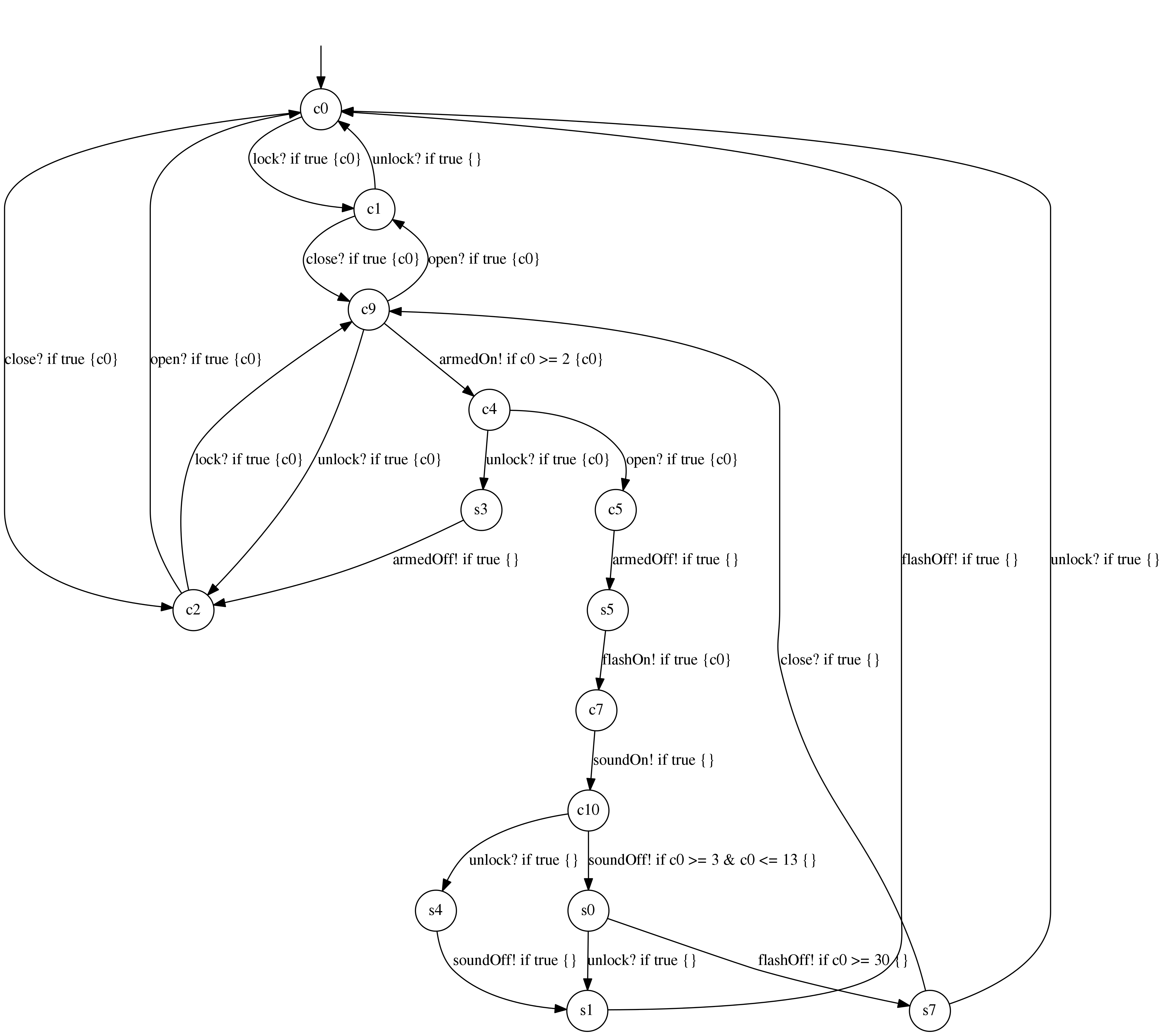
Figure 6: Learned model of the car alarm system (CAS).

Figure 6 shows a learned model of the CAS as it is produced by our tool (no post-processing). It is observably equivalent to the true system generating the timed traces used for learning. There is thus no test sequence which distinguishes the system from the learned model. Note that the model is also well comprehensible. This is due to the fitness penalty for larger systems and due to implicit input-enabledness. Both measures target the generation of small models containing only necessary information. The CAS model only contains a few unnecessary clock resets and an ineffective upper bound in the guard of the edge labelled soundOff!, but removing any edge would alter the observable behaviour. Therefore, our approach may enable manual inspection of black-box timed systems, which is substantially more difficult and labour-intensive given only observed timed traces.

V Conclusion

V-A Summary.

We presented an approach to learn deterministic TA with urgent outputs, an important subclass for testing timed systems [27]. The learned models may reveal flaws during manual inspection and enable verification of black-box systems via model-checking. Genetic programming, a meta-heuristic search technique, serves as a basis. In our implementation of it, we parallelise search by evolving two populations simultaneously and developed techniques for mutation, crossover, and for a fine-grained fitness-evaluation. We evaluated the technique on non-trivial TA with up to $26$ locations. We could learn all 44 TA models, only two random TA needed a small parameter adjustment.

V-B Related Work.

Verwer et al. [50, 51] passively learned real-time automata via state-merging. These TA measure the time between two consecutive events and use guards in the form of intervals, i.e. they have a single clock which is reset on every transition. Verwer et al.  do not distinguish between inputs and outputs, and hence, do not assume output urgency. Improvements of [51] were presented in [40]. Similarly, Mao et al. applied state-merging for learning continuous time Markov chains [39]. A state-merging-based learning algorithm for more general stochastic timed systems has been proposed by de Matos Pedro et al. [16]. They target learning generalised semi-Markov processes, which are generated by stochastic timed automata. All these techniques have in common that they consider timed systems where the relation between different events is fully described by a system’s structure. Pastore et al. [43] learn specifications capturing the duration of (nested) operations in software systems. A timed trace therefore includes for each operation its start and its end, i.e. the trace records two related events. Their algorithm Timed k-Tail is based on the passive learning technique k-Tail, which they extended to handle timing aspects.

Grinchtein et al. [23, 24] described active learning approaches for deterministic event-recording automata, a subclass of TA with one clock per action. The clock corresponding to an action is reset upon its execution essentially recording the time since the action has occurred. While the expressiveness of these automata suffices for many applications, the runtime complexity of the described techniques is high and may be prohibitive in practice. At the time of writing, there is no implementation to actually measure runtime. Furthermore, this kind of TA cannot model certain timing patterns, e.g., in the case of input enabledness where always reseting a clock may not be appropriate. Jonsson and Vaandrager [32] also note that the learning approaches presented previously [23, 24] are complex and developed a more practical active-learning approach for Mealy machines with timers. Currently, there is no implementation for this approach as well. A further drawback is that input edges cannot be restricted via guards.

Meta-heuristic search as an alternative to classical model learning such as $L^{*}$ has, e.g., been proposed by Lai et al. [35] in the context of adaptive model-checking. They apply genetic algorithms and assume the number of states to be known. Lucas and Reynolds in contrast compared state-merging and evolutionary algorithms, but also fixed the number of states for runs of the latter [38].

Lefticaru et al. similarly assume the number of states to be known and induce state machine models via genetic algorithms [37]. Their goal, however, is to synthesise a model satisfying a specification given in temporal logics. Early work suggesting such an approach was performed by Johnson [31], which like our approach does not require the solution size to be known. In contrast, Johnson does not apply crossover. Further synthesis work from Katz and Peled [33] tries to infer a correct program or model on the source code level, while we aim at synthesising a model representing a black-box system.

Evolutionary methods have been combined with testing in several areas: Abdessalem et al. [2] use evolutionary algorithms for the generation of test scenarios and learn decision trees to identify critical scenarios. Using the learned trees, they can steer the test generation towards critical scenarios. The tool Evosuite by Fraser and Arcuri [21] uses genetic operators for optimising whole test suites at once, increasing the overall coverage, while reducing the size of the test suite. Walkinshaw and Fraser presented Test by Committee, test-case generation using uncertainty sampling [53]. The approach is independent of the type of model that is inferred and an adaption of Query By Committee, a technique commonly used in active learning. In their implementation, they infer several hypotheses at each stage via genetic programming, generate random tests and select those tests which lead to the most disagreement between the inferred hypotheses. In contrast to most other works considered, their implementation infers non-sequential programs. It infers functions mapping from numerical inputs to single outputs.

The work by Steffen et al. [29, 47] is another good showcase for the strong possible relation between testing and model learning. They combine both areas, by performing black box tests and using the results to generate a model. Contrary to our work, they perform active learning, i.e., they use the intermediate versions of the learned models to guide the test generation. For a more comprehensive overview of combinations of learning and testing, we refer to [6].

V-C Future Work.

As indicated above, our technique is entirely passive, i.e. we learn from a set of timed traces (test observations), collected beforehand by random testing. There is no feedback from genetic programming to testing. In contrast to this, model-based testing could be applied to find discrepancies between the SUT and learned models [52]. These may then be used to iteratively refine the models. Active testing based on intermediate learned models may improve coverage of the SUT while requiring fewer tests, since we would benefit from additional knowledge about the system behaviour. This may therefore lead to improved accuracy of the model and increased performance through a reduction of tests and testing time. We are currently investigating possible implementations of active learning.

Assuming output urgency helps to approximate equivalence checks by “testing” candidate automata during learning. However, such models do not allow for uncertainty with respect to output timing. Relaxing this limitation represents an important next step. We are also currently working on this topic.

We demonstrated that TA can be genetically programmed, i.e. their structure is amenable to iterative refinement via mutation and crossover. Therefore, we could apply the same approach, but base the fitness evaluation on model checking by adapting the technique presented by Katz and Peled [33], to synthesise TA satisfying some properties. This would enable learning a black-box system, which may contain errors, and synthesising a controller ensuring that those errors do not lead to observable system failures.

References

- [1] 2017 IEEE International Conference on Software Testing, Verification and Validation, ICST 2017, Tokyo, Japan, March 13-17, 2017. IEEE, 2017.
- [2] Raja Ben Abdessalem, Shiva Nejati, Lionel C. Briand, and Thomas Stifter. Testing vision-based control systems using learnable evolutionary algorithms. In Proceedings of the 40th International Conference on Software Engineering, ICSE ’18, pages 1016–1026, New York, NY, USA, 2018. ACM.
- [3] Bernhard K. Aichernig, Jakob Auer, Elisabeth Jöbstl, Robert Korosec, Willibald Krenn, Rupert Schlick, and Birgit Vera Schmidt. Model-based mutation testing of an industrial measurement device. In Martina Seidl and Nikolai Tillmann, editors, Tests and Proofs - 8th International Conference, TAP 2014, Held as Part of STAF 2014, York, UK, July 24-25, 2014. Proceedings, volume 8570 of Lecture Notes in Computer Science, pages 1–19. Springer, 2014.
- [4] Bernhard K. Aichernig, Florian Lorber, and Dejan Nickovic. Time for mutants - model-based mutation testing with timed automata. In Margus Veanes and Luca Viganò, editors, Tests and Proofs - 7th International Conference, TAP 2013, Budapest, Hungary, June 16-20, 2013. Proceedings, volume 7942 of Lecture Notes in Computer Science, pages 20–38. Springer, 2013.
- [5] Bernhard K. Aichernig, Florian Lorber, and Martin Tappler. Conformance checking of real-time models - symbolic execution vs. bounded model checking. In Erika Ábrahám, Marcello M. Bonsangue, and Einar Broch Johnsen, editors, Theory and Practice of Formal Methods - Essays Dedicated to Frank de Boer on the Occasion of His 60th Birthday, volume 9660 of Lecture Notes in Computer Science, pages 15–32. Springer, 2016.
- [6] Bernhard K. Aichernig, Wojciech Mostowski, Mohammad Reza Mousavi, Martin Tappler, and Masoumeh Taromirad. Model learning and model-based testing. In Amel Bennaceur, Reiner Hähnle, and Karl Meinke, editors, Machine Learning for Dynamic Software Analysis: Potentials and Limits - International Dagstuhl Seminar 16172, Dagstuhl Castle, Germany, April 24-27, 2016, Revised Papers, volume 11026 of Lecture Notes in Computer Science, pages 74–100. Springer, 2018.
- [7] Bernhard K. Aichernig and Martin Tappler. Symbolic input-output conformance checking for model-based mutation testing. Electr. Notes Theor. Comput. Sci., 320:3–19, 2016.
- [8] Bernhard K. Aichernig and Martin Tappler. Learning from faults: Mutation testing in active automata learning. In NFM 2017, volume 10227 of LNCS, pages 19–34. Springer, 2017.
- [9] Rajeev Alur and David L. Dill. A theory of timed automata. Theor. Comput. Sci., 126(2):183–235, 1994.
- [10] George Argyros, Ioannis Stais, Suman Jana, Angelos D. Keromytis, and Aggelos Kiayias. SFADiff: Automated evasion attacks and fingerprinting using black-box differential automata learning. In Proceedings of the 2016 ACM SIGSAC Conference on Computer and Communications Security, pages 1690–1701. ACM, 2016.
- [11] Gerd Behrmann, Alexandre David, and Kim Guldstrand Larsen. A tutorial on Uppaal. In Marco Bernardo and Flavio Corradini, editors, Formal Methods for the Design of Real-Time Systems, International School on Formal Methods for the Design of Computer, Communication and Software Systems, SFM-RT 2004, Bertinoro, Italy, September 13-18, 2004, Revised Lectures, volume 3185 of Lecture Notes in Computer Science, pages 200–236. Springer, 2004.
- [12] Hans-Georg Beyer and Hans-Paul Schwefel. Evolution strategies - A comprehensive introduction. Natural Computing, 1(1):3–52, 2002.
- [13] Tobias Blickle and Lothar Thiele. A comparison of selection schemes used in evolutionary algorithms. Evolutionary Computation, 4(4):361–394, 1996.
- [14] Sébastien Bornot, Joseph Sifakis, and Stavros Tripakis. Modeling urgency in timed systems. In COMPOS’97. Revised Lectures, volume 1536 of LNCS, pages 103–129. Springer, 1997.
- [15] Colin de la Higuera. Grammatical Inference: Learning Automata and Grammars. Cambridge University Press, New York, NY, USA, 2010.
- [16] André de Matos Pedro, Paul Andrew Crocker, and Simão Melo de Sousa. Learning stochastic timed automata from sample executions. In Tiziana Margaria and Bernhard Steffen, editors, Leveraging Applications of Formal Methods, Verification and Validation. Technologies for Mastering Change - 5th International Symposium, ISoLA 2012, Heraklion, Crete, Greece, October 15-18, 2012, Proceedings, Part I, volume 7609 of Lecture Notes in Computer Science, pages 508–523. Springer, 2012.
- [17] Joeri de Ruiter and Erik Poll. Protocol state fuzzing of TLS implementations. In Jaeyeon Jung and Thorsten Holz, editors, 24th USENIX Security Symposium, USENIX Security 15, Washington, D.C., USA, August 12-14, 2015., pages 193–206. USENIX Association, 2015.
- [18] Edith Elkind, Blaise Genest, Doron A. Peled, and Hongyang Qu. Grey-box checking. In FORTE 2006, volume 4229 of LNCS, pages 420–435. Springer, 2006.
- [19] Paul Fiterau-Brostean, Ramon Janssen, and Frits W. Vaandrager. Combining model learning and model checking to analyze TCP implementations. In CAV 2016, Proceedings, Part II, volume 9780 of LNCS, pages 454–471. Springer, 2016.
- [20] Paul Fiterau-Brostean, Toon Lenaerts, Erik Poll, Joeri de Ruiter, Frits W. Vaandrager, and Patrick Verleg. Model learning and model checking of SSH implementations. In SPIN 2017, pages 142–151. ACM, 2017.
- [21] Gordon Fraser and Andrea Arcuri. Evosuite: automatic test suite generation for object-oriented software. In Proceedings of the 19th ACM SIGSOFT Symposium and the 13th European Conference on Foundations of Software Engineering, ESEC/FSE ’11, pages 416–419, New York, NY, USA, 2011. ACM.
- [22] Rodolfo Gómez. A compositional translation of timed automata with deadlines to UPPAAL timed automata. In FORMATS 2009. Proceedings, volume 5813 of LNCS, pages 179–194. Springer, 2009.
- [23] Olga Grinchtein, Bengt Jonsson, and Martin Leucker. Learning of event-recording automata. Theor. Comput. Sci., 411(47):4029–4054, 2010.
- [24] Olga Grinchtein, Bengt Jonsson, and Paul Pettersson. Inference of event-recording automata using timed decision trees. In CONCUR 2006, Proceedings, volume 4137 of LNCS, pages 435–449. Springer, 2006.
- [25] Alex Groce, Doron A. Peled, and Mihalis Yannakakis. Adaptive model checking. In TACAS 2002, Proceedings, volume 2280 of LNCS, pages 357–370. Springer, 2002.
- [26] Anders Hessel, Kim Guldstrand Larsen, Marius Mikucionis, Brian Nielsen, Paul Pettersson, and Arne Skou. Testing real-time systems using UPPAAL. In Robert M. Hierons, Jonathan P. Bowen, and Mark Harman, editors, Formal Methods and Testing, An Outcome of the FORTEST Network, Revised Selected Papers, volume 4949 of Lecture Notes in Computer Science, pages 77–117. Springer, 2008.
- [27] Anders Hessel, Kim Guldstrand Larsen, Brian Nielsen, Paul Pettersson, and Arne Skou. Time-optimal real-time test case generation using UPPAAL. In FATES 2003, volume 2931 of LNCS, pages 114–130. Springer, 2003.
- [28] Kassel Hingee and Marcus Hutter. Equivalence of probabilistic tournament and polynomial ranking selection. In CEC 2008, pages 564–571. IEEE, 2008.
- [29] H. Hungar, T. Margaria, and B. Steffen. Test-based model generation for legacy systems. In International Test Conference, 2003. Proceedings. ITC 2003., volume 2, pages 150–159 Vol.2, Sept 2003.
- [30] Malte Isberner, Falk Howar, and Bernhard Steffen. The open-source LearnLib - A framework for active automata learning. In CAV 2015, Proceedings, Part I, volume 9206 of LNCS, pages 487–495. Springer, 2015.
- [31] Colin G. Johnson. Genetic programming with fitness based on model checking. In EuroGP 2007, Proceedings, volume 4445 of LNCS, pages 114–124. Springer, 2007.
- [32] Bengt Jonsson and Frits W. Vaandrager. Learning Mealy machines with timers. online preprint, 2018. available via http://www.sws.cs.ru.nl/publications/papers/fvaan/MMT/, accessed 12 October 2018.
- [33] Gal Katz and Doron Peled. Synthesizing, correcting and improving code, using model checking-based genetic programming. STTT, 19(4):449–464, 2017.
- [34] John R. Koza. Genetic programming - on the programming of computers by means of natural selection. Complex adaptive systems. MIT Press, 1993.
- [35] Zhifeng Lai, S. C. Cheung, and Yunfei Jiang. Dynamic model learning using genetic algorithm under adaptive model checking framework. In QSIC 2006, pages 410–417. IEEE Computer Society, 2006.
- [36] Kim Guldstrand Larsen, Paul Pettersson, and Wang Yi. UPPAAL in a nutshell. STTT, 1(1-2):134–152, 1997.
- [37] Raluca Lefticaru, Florentin Ipate, and Cristina Tudose. Automated model design using genetic algorithms and model checking. In BCI 2009, pages 79–84. IEEE, 2009.
- [38] Simon M. Lucas and T. Jeff Reynolds. Learning DFA: evolution versus evidence driven state merging. In CEC 2003, pages 351–358. IEEE, 2003.
- [39] Hua Mao, Yingke Chen, Manfred Jaeger, Thomas D. Nielsen, Kim G. Larsen, and Brian Nielsen. Learning deterministic probabilistic automata from a model checking perspective. Machine Learning, 105(2):255–299, 2016.
- [40] Braham Lotfi Mediouni, Ayoub Nouri, Marius Bozga, and Saddek Bensalem. Improved learning for stochastic timed models by state-merging algorithms. In NFM 2017, volume 10227 of LNCS, pages 178–193. Springer, 2017.
- [41] Melanie Mitchell. An introduction to genetic algorithms. MIT Press, 1998.
- [42] Mariusz Nowostawski and Riccardo Poli. Parallel genetic algorithm taxonomy. In KES 1999, pages 88–92. IEEE, 1999.
- [43] Fabrizio Pastore, Daniela Micucci, and Leonardo Mariani. Timed k-tail: Automatic inference of timed automata. In 2017 IEEE International Conference on Software Testing, Verification and Validation, ICST 2017, Tokyo, Japan, March 13-17, 2017 [1], pages 401–411.
- [44] Doron A. Peled, Moshe Y. Vardi, and Mihalis Yannakakis. Black box checking. Journal of Automata, Languages and Combinatorics, 7(2):225–246, 2002.
- [45] Suphannee Sivakorn, George Argyros, Kexin Pei, Angelos D. Keromytis, and Suman Jana. HVLearn: Automated black-box analysis of hostname verification in SSL/TLS implementations. In SP 2017, pages 521–538. IEEE Computer Society, 2017.
- [46] Jan Springintveld, Frits W. Vaandrager, and Pedro R. D’Argenio. Testing timed automata. Theor. Comput. Sci., 254(1-2):225–257, 2001.
- [47] Bernhard Steffen, Falk Howar, and Maik Merten. Introduction to active automata learning from a practical perspective. In Formal Methods for Eternal Networked Software Systems - 11th International School on Formal Methods for the Design of Computer, Communication and Software Systems, SFM 2011, Bertinoro, Italy, June 13-18, 2011. Advanced Lectures, volume 6659 of LNCS, pages 256–296. Springer, 2011.
- [48] Martin Tappler, Bernhard K. Aichernig, and Roderick Bloem. Model-based testing IoT communication via active automata learning. In ICST 2017 [1], pages 276–287.
- [49] Martin Tappler and Andrea Pferscher. Supplementary Material for ”Learning Timed Automata via Genetic Programming”, 2018. https://figshare.com/articles/Supplementary_Material_for_Learning_Timed_Automata_via_Genetic_Programming_/5513575.
- [50] Sicco Verwer, Mathijs De Weerdt, and Cees Witteveen. An algorithm for learning real-time automata. In Benelearn 2007, 2007.
- [51] Sicco Verwer, Mathijs de Weerdt, and Cees Witteveen. A likelihood-ratio test for identifying probabilistic deterministic real-time automata from positive data. In ICGI 2010. Proceedings, volume 6339 of LNCS, pages 203–216. Springer, 2010.
- [52] Neil Walkinshaw, John Derrick, and Qiang Guo. Iterative refinement of reverse-engineered models by model-based testing. In FM 2009, volume 5850 of LNCS, pages 305–320. Springer, 2009.
- [53] Neil Walkinshaw and Gordon Fraser. Uncertainty-driven black-box test data generation. In 2017 IEEE International Conference on Software Testing, Verification and Validation, ICST 2017, Tokyo, Japan, March 13-17, 2017 [1], pages 253–263.