Updated astrometry and masses of the LUH 16 brown dwarf binary

The nearest known binary brown dwarf WISE J104915.57-531906.1AB (LUH 16) is a well-studied benchmark for our understanding of substellar objects. Previously published astrometry of LUH 16 obtained with FORS2 on the Very Large Telescope was affected by errors that limited its use in combination with other datasets, thereby hampering the determination of its accurate orbital parameters and masses. We improve upon the calibration and analysis of the FORS2 astrometry with the help of Gaia DR2 to generate a high-precision dataset that can be combined with present and future LUH 16 astrometry. We demonstrate its use by combining it with available measurements from the Hubble Space Telescope (HST) and Gemini/GeMS and deriving updated orbital and mass parameters. Using Gaia DR2 as astrometric reference field, we derived the absolute proper motion and updated the absolute parallax of the binary to 501.557$\pm$0.082 mas. We refined the individual dynamical masses of LUH 16 to $33.5\pm 0.3\,M_{Jup}$ (component A) and $28.6\pm 0.3\,M_{Jup}$ (component B), which corresponds to a relative precision of $\sim$1% and is three to four times more precise than previous estimates. We found that these masses show a weak dependence on one datapoint extracted from a photographic plate from 1984. The exact determination of a residual mass bias, if any, will be possible when more high-precision data can be incorporated in the analysis.

1 Introduction

After its discovery by Luhman (2013), the binary brown dwarf WISE J104915.57-531906.1 (Luhman 16, hereafter LUH 16) located at 2 pc from the Sun has been observed extensively. The astrometric follow-up by Boffin et al. (2014) used observations with the FORS2 camera on the Very Large Telescope (VLT) between April and June of 2013 to refine the parallax value to $2.020\pm 0.019$ pc and to claim indications for the presence of a massive substellar companion around one of the binary components.

Including additional epochs obtained in 2014 with FORS2, (Sahlmann & Lazorenko 2015) derived the relative (500.23 mas) and absolute parallax $\varpi_{\mathrm{abs}}=500.51\pm 0.11$ mas of this system, obtained an upper mass limit for a potential third body of 2$M_{\rm Jup}$, and determined a mass ratio $q=0.78\pm 0.10$ for the LUH 16 binary. After publication of Gaia Data Release 1 (DR1 Gaia Collaboration et al. 2016b, a; Lindegren et al. 2016), we updated the FORS2 distortion correction, which led to the updated values of $501.139$ mas and $\varpi_{\mathrm{abs}}=501.419\pm 0.11$ mas for the relative and absolute parallax, respectively (Lazorenko & Sahlmann 2017).

Using Hubble Space Telescope (HST) observations in 2014–2016, Bedin et al. (2017) derived a relative $501.118$ mas and absolute parallax $501.398\pm 0.093$ mas for LUH 16. Because of a longer observation time span, they were able to obtain estimates of the orbital elements of the system, in particular, $31.3\pm 7.9$ years for the orbital period and $0.463\pm 0.064$ for eccentricity. Bedin et al. (2017) found inconsistencies between their HST astrometry and the Sahlmann & Lazorenko (2015) astrometry at the level of 10–20 mas and therefore did not use FORS2 measurements for the orbit fitting.

Garcia et al. (2017) performed an independent analysis of the FORS2 observations obtained in 2013–2014 and added five more epochs in 2015, using Gaia DR1 for the transformation from CCD positions to the International celestial reference frame (ICRF). They added relative astrometry from the Gemini South Multiconjugate Adaptive Optics System (GeMS, Ammons et al. 2016), ESO photographic plates, CRIRES radial velocity, and archival observations from the Deep Near-Infrared Survey of the Southern Sky (DENIS). The HST astrometry was not published at that time and was not used.

Here we report new results from the combination of all available datasets, which increases the time span of high-precision astrometry from $\sim$2 years covered by the Bedin et al. (2017) study to 3.5 years. In comparison with our first study (Sahlmann & Lazorenko 2015), we present improved astrometric calibrations of the FORS2 data. We then update the orbital parameters and dynamical masses of the binary on the basis of a combination of FORS2, HST, GeMS, ESO archive, Gaia DR1, and Gaia DR2 (Lindegren et al. 2018; Gaia Collaboration 2018) astrometry, and the CRIRES relative radial velocity to constrain the inclination.

2 FORS2 astrometry

2.1 Observational data

We used imaging observations obtained with three large telescopes. This dataset contains 22 FORS2 frame series in 2013–2014 obtained by Boffin et al. (2014) with the high-resolution mode and a 0.126″/px pixel scale. The dates of observations and the average full width at half-maximum (FWHM) are given in Table 1. The 2015 observations were obtained when the relative binary separation was $\sim$0.7″, which is too small for very precise astrometry, and we therefore did not use these data.

Table 1: Dates of FORS2 observations, average FWHM ${\varepsilon}$ (in arcseconds), and DCR-related functions used in Eq. (1).

epoch	Year	${\varepsilon}$	$f_{1,x}$	$f_{2,x}$	$f_{1,y}$	$f_{2,y}$
1	2013.28541	0.62	-0.6030	-0.7187	-0.4672	-0.5568
2	2013.29928	0.67	-0.0476	-0.0585	-0.5484	-0.6746
3	2013.31565	0.55	-0.0724	-0.0873	-0.5477	-0.6602
4	2013.34301	0.87	0.0541	0.0656	-0.5482	-0.6644
5	2013.35959	0.79	0.5369	0.6555	-0.4838	-0.5907
6	2013.38392	0.83	-0.0526	-0.0656	-0.5483	-0.6835
7	2013.39776	0.64	0.4096	0.5067	-0.5108	-0.6319
8	2013.41408	0.69	0.2562	0.3176	-0.5339	-0.6620
9	2013.42505	0.71	0.3719	0.4497	-0.5175	-0.6257
10	2013.43866	0.68	0.2840	0.3391	-0.5305	-0.6334
11	2013.44969	0.73	0.5133	0.6454	-0.4894	-0.6152
12	2013.45784	0.69	0.4349	0.5260	-0.5060	-0.6119
13	2013.47425	0.90	0.4995	0.6075	-0.4925	-0.5989
14	2014.09650	0.72	-0.1541	-0.1876	-0.5436	-0.6619
15	2014.12097	0.58	-0.3863	-0.4714	-0.5151	-0.6285
16	2014.18656	0.72	-0.2443	-0.2937	-0.5354	-0.6436
17	2014.21130	0.80	0.1625	0.1985	-0.5430	-0.6632
18	2014.24126	0.68	-0.0222	-0.0272	-0.5489	-0.6737
19	2014.27135	0.68	0.1208	0.1465	-0.5457	-0.6618
20	2014.31484	0.64	-0.3605	-0.4392	-0.5194	-0.6327
21	2014.34219	0.88	-0.2521	-0.3028	-0.5345	-0.6419
22	2014.37776	0.80	-0.0450	-0.0548	-0.5486	-0.6681

We used the 36 HST measurements published in Bedin et al. (2017) that were obtained with the Wide Field Camera 3 in 2014–2016, which increases the total time span of high-precision observations to 3.5 years with approximately even sampling. This dataset is supplemented with six series of images obtained by Ammons et al. (2016) in 2014–2015 with Gemini/GeMS. Because GeMS uses adaptive optics, it produces well-separated and therefore well-measured images of the components. In addition, these infrared observations have low sensitivity to differential chromatic refraction (DCR) effects. Some GeMS images were taken close in time to FORS2 epochs, which is useful to independently control the quality of calibrations in the FORS2 astrometry. The ESO archive contains some more archived images, for example, photographic R-band images obtained with the Schmidt telescope in 1984. We used these data, reduced to ICRF by Garcia et al. (2017), to improve the quality of our reduction. In total, we used 64 frame series covering 3.5 years, and one more distant epoch of ESO-R in 1984.

Gaia DR2 includes two-parameter solutions, that is, positions only, for the two components of LUH 16. The identifiers are Gaia DR2 5353626573562355584 for LUH 16 A and Gaia DR2 5353626573555863424 for LUH 16 B. Because of the large astrometric uncertainties (2–47 mas) and the potential biases in the DR2 positions due to unaccounted orbital motion and blending, we did not use these data in our analysis.

2.2 Layout of investigation

Several studies (Boffin et al. 2014; Sahlmann & Lazorenko 2015; Garcia et al. 2017) used the same FORS2 dataset (Table 1) but arrived at discrepant astrometric results. This illustrates the difficulties of ground-based sub-milliarcsecond astrometry, which are related to DCR, biases in measuring positions of close binary components, and other effects analyzed below.

Here we aim at mitigating these effects. We begin with a basic astrometric reduction applied to the FORS2 observations, which mitigates atmospheric image motion, geometric field distortion, DCR, and other effects to a level of about 0.1 mas. We started from the measured positions of stars $x^{\prime}$, $y^{\prime}$ obtained in our previous study Sahlmann & Lazorenko (2015). The reduction was performed in a sequence of repeating steps, which is necessary to estimate the optimal radius of the reference field and remove systematic errors (Sahlmann et al. 2014; Lazorenko et al. 2011, 2014).

The following analysis is specific to LUH 16, and we used FORS2, HST, and GeMS observations to apply a model that includes new calibrations of the FORS2 measurements. Solutions were derived iteratively by splitting the full model into independent blocks, finding approximate solutions for model parameters within these blocks, and repeating computations until converging to the final solution. This expanded model includes

• five astrometric parameters $x_{c}$, ${y}_{c}$, $\mu_{x}$, $\mu_{y}$, $\varpi$ for the barycenter motion of the binary,

• two DCR parameters $\rho$, $d$, which affect the barycenter motion as seen through the atmosphere (FORS2 only)

• seven orbital elements,

• the mass ratio $q$,

• 12 parameters $k_{0}^{x}\ldots k_{2}^{x}$, $k_{0}^{y}\ldots k_{2}^{y}$, for each binary component and each annual period, to calibrate for the bias in positions caused by the seeing and flux variations (FORS2 only),

• offset $\varepsilon_{0}$ for the effective average seeing (FORS2 only),

• two calibration parameters to remove the offsets between the equatorial positions of the binary barycenter of FORS2 and HST.

In Sect. 2.3 we describe the transformation of the measured positions $x^{\prime}$, $y^{\prime}$ to raw $x_{raw}$, $y_{raw}$ positions of each LUH 16 component in the reference frame of FORS2, free of the optical distortions. The positional residuals $\Delta^{\prime}$ of the least-squares fit derived at this step provide information on the relative displacement of CCD chips (Lazorenko et al. 2014), the residual correlations in the CCD space (Sect. 2.4), and on variations with seeing (Sect. 2.5). Calibration of these effects produces ‘clean‘ astrometric positions $\bar{x}$, $\bar{y}$, that are still affected by DCR, however (Sect. 2.5). Some of the above calibrations require knowledge of the orbital motion of the LUH 16 components on the sky, however, which was derived by iteration starting from a rough initial approximation.

The FORS2 and HST/GeMS positions were obtained in different reference systems. Whereas the FORS2 reference frame is local and set by the field stars, the HST/GeMS positions are given in ICRF. Therefore, adopting ICRF as a common system for this investigation, we transformed $\bar{x}$, $\bar{y}$ to positions $x_{A}$, $y_{A}$, $x_{B}$, and $y_{B}$ for each A and B component in ICRF (Sect. 2.6). These positions, combined with HST and GeMS data, were used to derive the solution for the orbital and barycenter motion (Sect. 3).

2.3 Basic astrometric reductions

To reduce the FORS2 observations, we employed our usual method, which ensures an astrometric precision of about 0.1 mas for isolated sources (Sahlmann et al. 2014; Lazorenko et al. 2011, 2014). The measured photocenter positions ${x}^{\prime}$ and ${y}^{\prime}$ for every star in the field (reference or target) imaged at time $t$ are represented by the model

$$\begin{array}[]{@{}l}x_{0}+\hat{x}_{0}+{\Phi}_{x}(x^{\prime},y^{\prime})+\hat{\mu}_{x}(t-t_{0})+\hat{\varpi}p_{x}-\hat{\rho}f_{1,x}-\hat{d}f_{2,x}={x}^{\prime}\\ y_{0}+\hat{y}_{0}+{\Phi}_{y}(x^{\prime},y^{\prime})+\hat{\mu}_{y}t(t-t_{0})+\hat{\varpi}p_{y}+\hat{\rho}f_{1,y}+\hat{d}f_{2,y}={y}^{\prime}\end{array},$$ (1)

which describes the displacement of the stellar photocenter in the three-dimensional space formed by the coordinate axes $x$, $y$ oriented along RA, Dec, and time $t$. Here $x_{0}$, $y_{0}$ are the approximate CCD reference star positions, which are fixed and define the directions for the coordinate axes $x$, $y$ of the reference frame at the adopted reference time $t_{0}=56500$ MJD (=J2013.56742) close to the average epoch. Eq. (1) is solved by the least-squares fit, using all available measurements of reference stars. This yields seven astrometric parameters for each star: the coordinate offsets $\hat{x}_{0}$ and $\hat{y}_{0}$, the proper motion $\hat{\mu}_{x}$ and $\hat{\mu}_{y}$, the relative parallax $\hat{\varpi}$, the DCR index $\hat{\rho}$ describing atmospheric displacement of the stellar image depending on the star’s color, and the reverse displacement $d$, produced by the longitudinal atmospheric dispersion compensator (LADC) (Avila et al. 1997). Eq. (1) also contains the parallax factors $p_{x}$, $p_{y}$ and the DCR related functions $f_{1,x}=\tan z\sin\gamma$, $f_{1,y}=\tan z\cos\gamma$, $f_{2,x}=\tan z_{\rm L}\sin\gamma$, and $f_{2,y}=\tan z_{\rm L}\cos\gamma$, where $z$ is the zenith distance, $z_{\mathrm{L}}$ is the LADC parameter, and $\gamma$ is an angle between direction to zenith and north.

The key component of Eq. (1) is the function $\Phi(x^{\prime},y^{\prime})$, which is derived from reference stars only and models the sum of atmospheric image motion and geometric distortion variations for each individual frame. It is a full polynomial of order $k/2-1,$ where the model parameter $k$ is an even integer between 4 and 16. Here we set $k=10$ as the value that yields the most stable results. Using solution for $\Phi(x^{\prime},y^{\prime})$, we determined raw positions

$$x_{raw}=x^{\prime}-{\Phi}_{x}(x^{\prime},y^{\prime});\quad y_{raw}={y^{\prime}}-{\Phi}_{y}(x^{\prime},y^{\prime})$$ (2)

of each A and B component in the reference frame, which are the measured positions free of geometric distortion variations. Then from Eq. (1) we derived all astrometric parameters of the target objects (coordinate offsets, proper motion, parallax, and DCR parameters).

The LUH 16 components perform a nonlinear motion in the sky that is due to the curvature of the orbit, and the positional residuals $x_{raw}$, $y_{raw}$ display the measurement of the orbital segment $\psi$ expressed as $\psi_{x}=BX+GY$, $\psi_{y}=AX+FY$ with the Thiele-Innes parameters $A$, $B$, $F$, and $G$. The measured segment represents the residual of $\psi$ affected by the least-squares fit (Eq. 1). Because of the correlation between the parameters of the system Eq.(1) with $\psi$, their estimates are significantly biased. To emphasize this feature, we assigned a ’hat’ to the parameters of Eq. (1), in contrast to the ’actual’ corresponding parameters introduced later. The effect is illustrated by the difference of 3.53 mas in parallax values derived for components A and B with this preliminary approach, which is larger than the measurement uncertainty of 0.07 mas and is unphysical.

2.4 Correlations across CCD

The raw positions $x_{raw}$, $y_{raw}$ were corrected for space-dependent systematic errors as described below. The residuals $\Delta$ of the least-squares fit of Eq. (1) for reference stars are nearly random values with a scatter that corresponds to a typical FORS2 astrometric precision of 0.1–0.2 mas. However, they quite often display a correlation pattern of different type across CCD space. These correlations are traced and used to calibrate the raw positions in Eq. (2) of LUH 16 for similar systematic errors. In this way, we detected and removed the relative displacement between CCD chips 1 and 2, which can affect the positions by 1–2 mas. Another type of systematic errors is seen as an oscillating autocorrelation function across CCD space. Correlations occur as a natural consequence of the polynomial fit of any measurements limited in space and therefore are not specific for FORS2. For stars without orbital motion, these errors were mitigated as described in (Lazorenko et al. 2014), but for LUH 16, the effect is masked by the dominating signal $\psi,$ which should first be subtracted from $\Delta^{\prime}$. As an initial approximation for $\psi$, we used polynomials of time that smoothen the individual residuals $\Delta^{\prime}$ within each annual period, allowing us to form the corrected residuals $\Delta^{\prime}-\psi,$ which were then investigated and calibrated for errors correlated across the CCD. Later on, we used the actual signal $\psi$ to refine the calibrations iteratively.

2.5 Correlation of FORS2 positions with seeing

The images of the components of LUH 16A and LUH 16B partly overlap because the separation between the sources (1.4″on 2013 and 1.0″and 2014) was comparable to the FWHM (Table 1), which was about 0.69″ in RA and 0.76″ in Dec on average for both periods. We therefore expect that the measurements of CCD positions can be biased depending on seeing. This effect should cause a correlation between the positional residuals and the seeing for individual images.
We found that this correlation is of low significance when determined for individual frame series, therefore we split the data into the years 2013 and 2014, during which the separation between the A and B components changed only little. To fit the measured positional residuals $\Delta^{\prime}_{x}-\psi_{x}$ and $\Delta^{\prime}_{y}-\psi_{y}$ separately for 2013 and 2014, we used the linear expressions

$$\begin{array}[]{@{}ll}H_{x}(\varepsilon_{x},I)=k_{0}^{x}+k_{1}^{x}[\varepsilon_{x}-(\bar{\varepsilon}+\varepsilon_{0})]+k_{2}^{x}(I/I_{0}-1)\\ H_{y}(\varepsilon_{y},I)=k_{0}^{y}+k_{1}^{y}[\varepsilon_{y}-(\bar{\varepsilon}+\varepsilon_{0})]+k_{2}^{y}(I/I_{0}-1)\\ \end{array},$$ (3)

where $\varepsilon_{x}$ and $\varepsilon_{y}$ stand for the FWHM along $x$ and $y$ axes, $\bar{\varepsilon}$ is the average FWHM for the annual period, $\varepsilon_{0}$ is an offset discussed below, and $k_{0}$, $k_{1}$, and $k_{2}$ are the free model parameters. In addition to the linear dependence on $\varepsilon$, the model Eq.(3) includes a small but statistically significant component proportional to the change in flux $I$ in the image relative to its annual average flux $I_{0}$.

Table 2: Coefficients of Eq.(3) of the systematic bias in the photocenter position of components A and B.

	$k_{1}^{x}$	$k_{2}^{x}$	$k_{1}^{y}$	$k_{2}^{y}$
	(mas/arcsec)	(mas)	(mas/arcsec)	(mas)
year	component A
2013	1.58 $\pm$ 0.45	-0.19 $\pm$ 0.23	-0.26 $\pm$ 0.63	-0.74$\pm$ 0.31
2014	4.35 $\pm$ 0.45	-0.32 $\pm$ 0.29	-1.90 $\pm$ 0.47	-0.65$\pm$ 0.27
year	component B
2013	-4.30 $\pm$ 0.51	-0.71 $\pm$ 0.24	6.06 $\pm$ 0.69	-0.48$\pm$ 0.31
2014	-4.96 $\pm$ 0.56	1.45 $\pm$ 0.34	5.41 $\pm$ 0.50	-0.93$\pm$ 0.28

The coefficients $k_{0}$, $k_{1}$, and $k_{2}$ determined by the least-squares fit of the residuals $\Delta^{\prime}-\psi$ with the functions (3) were used to correct the measured values $x^{\prime}$, $y^{\prime}$, ${x_{raw}}$, and ${y_{raw}}$, thus obtaining the positions

$$\bar{x}=x_{raw}-H_{x}(\varepsilon_{x},I)\quad\bar{y}=y_{raw}-H_{y}(\varepsilon_{y},I),$$ (4)

which correspond to the average observational conditions set by $\bar{\varepsilon}$ and $I_{0}$. In this way, we decreased the internal scatter of the positional residuals within each frame series and within each annual period, but did not change their average values in 2013 and 2014 significantly, thus the orbital parameters are hardly affected by this correction.

However, this does not yet solve the problem because the measurements that are not biased by seeing should correspond not to $\bar{\varepsilon}$ but to $\varepsilon=\bar{\varepsilon}+\varepsilon_{0}$ offset to a better seeing by some unknown value $\varepsilon_{0}$. The key parameters derived at this phase of the reduction are the linear coefficients $k_{1,x}$ and $k_{1,y}$ (for components A and B each) used later to determine $\varepsilon_{0}$ in Sect. 3 as a free parameter of the relative orbital motion.

The derived coefficients of Eq.(3) except for the offsets $k_{0}$ are given in Table 2. These coefficients were initially obtained with the residuals $\Delta^{\prime}-\psi$ using a polynomial approximation of $\psi$. Then we iteratively improved this estimate by applying $\psi$ derived for the full solution of the orbital motion. We note that the coefficients $k_{1}$ are larger for component B, as expected, because it is fainter, and they are approximately equal for both annual periods because the distance between the components did not change much. The values have opposite signs for components A and B. Considering the sign of $k_{1}$, this means that for poor seeing, the measured positions of the components are offset in the direction away from the other component. The amplitude of the corrections in the positions for the maximum variations in seeing of about $\pm 0.2$″  can reach $\pm 1$ mas, which significantly exceeds the measurement uncertainty.

Table 3: FORS2 Cartesian measured positions $x_{A}$, $y_{A}$ of the A and $x_{B}$, $y_{B}$ of the B component, corrected for variations of seeing and flux (assuming that $\varepsilon_{0}=0$), but including the DCR displacements and the measurement uncertainties $\sigma_{A}$, $\sigma_{B}$. Positions $x^{*}_{A}$, $y^{*}_{A}$, $x^{*}_{B}$, $y^{*}_{B}$ are corrected for DCR, for the offsets $\Delta_{x}$, $\Delta_{y}$ given in Table 7, and for $\varepsilon_{0}=-0.192$″. Positions are linked to ICRF relative to the reference position $\alpha_{0}=162.3107300\degr$, $\delta_{0}=-53.3181500\degr$ and expressed in mas.

	Cartesian measured positions Eq.(5)						Cartesian corrected positions Eq.(9)				Relative positions
epoch	$x_{A}$	$y_{A}$	$\sigma_{A}$	$x_{B}$	$y_{B}$	$\sigma_{B}$	$x^{*}_{A}$	$y^{*}_{A}$	$x^{*}_{B}$	$y^{*}_{B}$	$x^{*}_{B}-x^{*}_{A}$	$y^{*}_{B}-y^{*}_{A}$
1	948.159	-470.565	0.168	-96.714	533.782	0.186	961.003	-480.931	-80.846	520.734	-1041.850	1001.664
2	892.440	-427.278	0.112	-148.442	573.002	0.146	893.355	-440.483	-146.242	556.831	-1039.597	997.314
3	815.484	-379.241	0.129	-222.726	616.691	0.161	816.892	-391.732	-219.955	601.255	-1036.847	992.987
4	700.253	-294.262	0.135	-333.117	693.398	0.171	698.817	-306.945	-333.591	677.763	-1032.407	984.708
5	645.418	-241.530	0.165	-383.083	741.177	0.198	632.783	-252.979	-396.289	726.973	-1029.073	979.952
6	543.313	-160.993	0.125	-482.652	815.556	0.163	544.391	-174.662	-480.272	798.908	-1024.663	973.569
7	508.819	-117.213	0.155	-513.252	855.337	0.188	498.790	-129.712	-523.457	839.986	-1022.247	969.698
8	455.684	-62.883	0.165	-563.765	903.971	0.199	449.296	-76.012	-569.840	887.914	-1019.136	963.926
9	426.926	-28.830	0.133	-589.991	934.574	0.168	418.335	-40.744	-598.623	919.806	-1016.958	960.550
10	389.562	13.531	0.096	-624.969	973.095	0.138	383.173	1.737	-631.115	958.418	-1014.288	956.681
11	370.447	47.682	0.118	-641.358	1003.940	0.152	357.397	35.189	-654.930	988.649	-1012.328	953.460
12	349.497	71.526	0.119	-661.631	1025.470	0.155	339.482	59.864	-671.887	1010.992	-1011.369	951.127
13	318.666	118.700	0.128	-688.965	1067.789	0.164	307.021	107.171	-701.060	1053.481	-1008.080	946.310
14	-842.125	-244.181	0.096	-1719.878	508.402	0.133	-839.329	-256.607	-1714.799	492.844	-875.470	749.451
15	-985.044	-242.271	0.076	-1858.255	501.228	0.119	-976.862	-254.106	-1847.053	486.348	-870.191	740.455
16	-1360.813	-184.604	0.086	-2217.756	536.883	0.128	-1356.139	-196.414	-2210.519	521.978	-854.380	718.392
17	-1493.606	-142.295	0.093	-2344.012	570.673	0.134	-1498.115	-154.812	-2347.243	555.022	-849.128	709.834
18	-1664.867	-79.152	0.087	-2509.057	623.308	0.132	-1665.090	-91.972	-2507.415	607.332	-842.325	699.303
19	-1821.348	-4.898	0.081	-2657.438	687.157	0.125	-1824.836	-17.232	-2659.514	671.687	-834.679	688.919
20	-2045.156	119.769	0.078	-2872.045	796.582	0.119	-2037.609	107.888	-2861.560	781.644	-823.951	673.756
21	-2161.897	205.624	0.099	-2982.425	873.325	0.136	-2157.066	193.868	-2975.007	858.478	-817.940	664.610
22	-2294.995	322.713	0.086	-3105.068	977.118	0.122	-2294.703	310.170	-3102.839	961.426	-808.136	651.256

2.6 Transformation into ICRF

It is convenient to perform the following analysis in the observational plane, where we have derived positions Eq. (4) related to the FORS2 reference frame. The metric of this frame, however, is deformed by the optical distortion and other effects that are significant even at the small separation between the LUH 16 components. Therefore we transformed these positions into an absolute system that is now well represented by the Gaia source catalogs of DR1 (Lindegren et al. 2016) or DR2 (Lindegren et al. 2018). As a suitable epoch for the transformation we adopted the epoch $T_{\mathrm{DR1}}$=J2015.0. The Gaia DR1 catalog was also used by Bedin et al. (2017) and Garcia et al. (2017) as reference to measure the positions of LUH 16. In this way, we obtained all positions in the ICRF at the epoch $T_{\mathrm{DR1}}$.

2.6.1 Transformation to the DR1 epoch

As explained in Lazorenko & Sahlmann (2017), the transformation was made only with stars imaged on the upper chip because the bottom CCD chip2 of FORS2 is rotated and shifted relative to the upper chip1, and the use of both chips leads to large residuals of about 50 mas. We tangent-plane projected the Gaia equatorial coordinates to the CCD plane at the point $X_{0}=1025.739$, $Y_{0}=109.640$ px near the position of LUH 16 in chip1 at the average time of observations, which corresponds to $\alpha_{0}=162.31073\degr$, $\delta_{0}=-53.31815\degr$, and compared the projected Gaia DR1 and DR2 source positions with those in the FORS2 reference system. Positions of DR2 were computed at the epoch $T_{\mathrm{DR1}}$ using the DR2 proper motions. To bridge the epoch difference between the reference epoch $t_{0}$ of FORS2 and the comparison epoch $T_{\mathrm{DR1}}$, we corrected the FORS2 positions with proper motions $\hat{\mu}_{x}$, $\hat{\mu}_{y}$ of Eq.(1) known with about twice better internally consistent precision as compared to DR2 (but systematically offset from the absolute, see Sect.  2.6.2).

The following least-squares fit of positional residuals was made with functions $F_{n}^{x}(\bar{x}-X_{0},\bar{y}-Y_{0})$ for RA, and $F_{n}^{y}(\bar{x}-X_{0},\bar{y}-Y_{0})$ for Dec, which are a sum of two-dimensional polynomials of the maximum power $n$ formed on coordinates $\bar{x}-X_{0}$ and $\bar{y}-Y_{0}$ of reference stars only. We tested all polynomial orders, starting from a linear model with $n=1$. The optimal order $n=4$ was found by using an F-test for the rejection of non-significant coefficients as described in (Lazorenko & Sahlmann 2017). Thus, using 79 stars identified as common between FORS2 and DR2 on the upper chip, we obtained the average rms of the residuals of 1.10 mas, which is approximately consistent with an average uncertainty 0.67 mas for Gaia DR2 stars and 0.38 mas for FORS2 stars at this epoch. A similar transformation was also made with DR1. In this case, with 73 common stars, the average rms of the residuals DR1 - FORS2 increased to 2.03 mas, which is explained by the larger uncertainty of the DR1 positions. In the following, we proceed with the results based on Gaia DR2.

With above procedure, we derived coefficients of functions $F_{n}^{x}$, $F_{n}^{y}$. Then, for each epoch of observations, we computed rectangular positions of LUH 16 A and B linked to the ICRF, which along RA are computed as

$$x_{A}=\bar{x}_{A}+F_{n}^{x}(\bar{x}_{A}-X_{0},\bar{y}_{B}-Y_{0}),x_{B}=\bar{x}_{B}+F_{n}^{x}(\bar{x}_{B}-X_{0},\bar{y}_{B}-Y_{0}).$$ (5)

The expressions for $y_{A}$, $y_{B}$ along Dec are similar. The transformation uncertainty, which depends on the covariation function of $F_{n}$, is 0.21 mas for the stars in the center of the reference field, but it degrades to 0.43 mas for our targets located at the edge of this field (we recall that this reference field is not centered on the target because all stars in chip2 were rejected). When the transformation to the common system is made with DR1, these uncertainties are about twice larger. The computed positions Eq. (5) may differ, within the above uncertainty limits, by some offset $\Delta$ from the ‘real’ positions in ICRF computed with error-free function $F_{n}$. Considering that the function $F_{n}$ changes slowly across the CCD, we can assume that this offset is approximately equal for components A and B and for all their measurements at different epochs. The offset $\Delta$, if exists, is canceled out in the distances between the components, but affects the barycenter position by $\Delta$. Because its value can be non-negligible, we included $\Delta$ in the model Eq. (6) for the motion of LUH 16.

For similar reasons, the HST positions of Bedin et al. (2017) can be offset from the ICRF by about 0.3 mas, thus we expect to find systematic discrepancies between FORS2 and HST measurements by $\sim 0.5$ mas.

In the left columns of Table 3 we give the positions Eq.(5), linked to the ICRF, that are affected by the DCR and reduced to the average seeing and flux with Eq.(3) and the coefficients from Table 2, assuming that $\varepsilon_{0}=0$.

2.6.2 Conversion of proper motions and parallaxes to absolute motions and parallaxes

By definition, the differential proper motions $\hat{\mu}$ and parallaxes $\hat{\varpi}$ of FORS2 systematically differ from their absolute values $\mu(\mathrm{abs})$ and $\varpi(\mathrm{abs})$ by some constant offsets $\Delta\mu$ and $\Delta\varpi$, thus $\mu(\mathrm{abs})=\hat{\mu}+\Delta\mu$ and $\varpi(\mathrm{abs})=\hat{\varpi}+\Delta\varpi$ (Lazorenko et al. 2009, 2014). While this is not important for deriving the relative angular motion of the binary, these parameters of the barycenter derived in Sect. 3.2 need to be corrected to absolute values. In our previous studies of nearby sources (e.g., Sahlmann et al. 2014), we derived statistical corrections for the FORS2 relative parallaxes $\varpi$ by comparing our data with a galaxy model (Robin et al. 2003). For LUH 16 we thus derived the correction term $\Delta\varpi=0.28\pm 0.01$ mas (Sahlmann & Lazorenko 2015).

With the availability of Gaia DR2, it becomes possible to determine the parallax correction by directly comparing the FORS2 and DR2 parallaxes of field stars. We used only those stars that define the system of FORS2 astrometric parameters (Lazorenko et al. 2014, Sect. 3.3.1); they are typically brighter than $G=20$. Because we used equal weights $P_{i}$ in Lazorenko et al. (2014, Eq.2) for these stars, the estimate of $\Delta\varpi$ is the simple arithmetic average offset. There were 65 stars in chip1 and 32 stars in chip2 that were also reduced to ICRF specifically for the purpose of deriving $\Delta\varpi$ and $\Delta\mu$. This direct comparison (Fig. 1, upper panel) yields a parallax correction value of $\varpi_{\mathrm{D}R2}-\varpi_{\mathrm{F}ORS2}=\Delta\varpi=0.342\pm 0.056$ mas, which within error bars agrees with the value reported by Sahlmann & Lazorenko (2015), thereby indirectly validating the model of (Robin et al. 2003) and our previous statistical method of deriving $\Delta\varpi$ at a level of $\pm 0.1$ mas in this field.

This assessment does not account for the DR2 parallax zero-point of $-29\,\mu$as discussed in Lindegren et al. (2018), which was determined for quasars and may be variable in amplitude as a function of magnitude, position, and other parameters. Since Gaia parallaxes are therefore too small, the DR2 zero-point offset increases the value of the parallax correction we derive by the equivalent amount.

In a similar way, we compared the proper motions in RA and obtained a linear dependence $\mu_{x}(\mathrm{DR2})=\Delta\mu_{x}+c_{x}\mu_{x}(\mathrm{FORS2})$ with an offset $\Delta\mu_{x}=-6.618\pm 0.111$ mas/yr and a nearly unity coefficient $c_{x}=0.953\pm 0.037$ mas/yr (Fig. 1). The RMS of the fit residuals of $1.1$ mas/yr is small but exceeds the uncertainties of 0.18 and 0.47 mas/yr for proper motions of FORS2 and DR2, respectively. In Dec, using the similar relation $\mu_{y}(\mathrm{DR2})=\Delta\mu_{y}+c_{y}\mu_{x}(\mathrm{FORS2})$, we derived $\Delta\mu_{x}=2.103\pm 0.120$ mas/yr, $c_{y}=0.957\pm 0.052$ mas/yr, and a residual scatter of $1.2$ mas/yr. The calibration terms $\Delta\mu_{x}$, $\Delta\mu_{y}$, and $\Delta\varpi$ determined here were used later in Sect. 3.2 to convert the relative barycenter proper motion and parallax into the absolute values, neglecting potential Gaia DR2 proper motion zero-point offsets.

Figure 1: Comparison between relative FORS2 and absolute DR2 parallaxes (upper panel) and proper motions in RA (lower panel) for brighter (filled circles; they were used to determine the correction) and fainter stars (open circles), with linear fit functions (solid lines).

3 Barycenter and orbital motion

The measured positions $x_{A}$, $y_{A}$ $x_{B}$, $y_{B}$ derived with Eq.(5) contain directly measured target positions, all calibrations for the effects described above, and although it is not explicitly evident, contain a full information on all measurements of the reference stars. The reference data were not discarded because they were integrated into the basic astrometric model and then were extracted again at any exposure moment and any CCD pixel in a refined form, for instance, filtered from the atmospheric image motion.

The measured positions from Eq.(5) were modeled by the sum of the barycenter motion of the system and its orbital motion in RA,

$$\begin{array}[]{@{}l@{}l}x_{A}=&x_{c}+\mu_{x}(t-t_{0})+\varpi p_{x}+\lambda(-\rho_{A}f_{1,x}-d_{A}f_{2,x}-k^{x}_{1,A}\varepsilon_{0})\\ &+BX+GY+\Delta_{x}\\ x_{B}=&x_{c}+\mu_{x}(t-t_{0})+\varpi p_{y}+\lambda(-\rho_{B}f_{1,x}-d_{B}f_{2,x}-k^{x}_{1,B}\varepsilon_{0})\\ &-Bq^{-1}X-Gq^{-1}Y+\Delta_{x},\\ \end{array},$$ (6)

and similar for the positions in Dec $y_{A}$, $y_{B}$. The model includes coordinate offsets $x_{c}$, $y_{c}$, proper motion $\mu_{x}$$(=\mu_{\alpha}\cos\delta)$, $\mu_{y}$, relative parallax $\varpi$, Thiele-Innes parameters $A$, $B$, $F$, and $G$, and the mass-ratio $q$. The DCR parameters $\rho_{A}$, $\rho_{B}$, $d_{A}$, $d_{B}$, and the offset $\varepsilon_{0}$ to the average FWHM from Eq.(3) are applicable to FORS2 only, which we flag by $\lambda=1$ for FORS2, and $\lambda=0$ in the other cases. The constants $\Delta_{x}$, $\Delta_{y}$ are defined in the previous Sect. 2.6.1 and are the systematic offsets to the positions $x_{A}$, $y_{A}$, $x_{B}$, $y_{B}$, which depend on the instrument. These equations can therefore contain $\Delta_{x}(\mathrm{HST})$, $\Delta_{x}(\mathrm{FORS2})$, $\Delta_{y}(\mathrm{HST}),$ or $\Delta_{y}(\mathrm{FORS2})$. Because the observational information for GeMS is insufficient, we assumed that $\Delta(\mathrm{GeMS})=0$.

From Eq. (6) we can obtain an expression for the barycenter motion in the sky that is independent of the orbital parameters, and an expression for the orbital motion that is independent of the barycenter motion. For the orbital motion, we have

$$\begin{array}[]{@{}ll}x_{B}-x_{A}=&\lambda[-(\rho_{B}-\rho_{A})f_{1,x}-(d_{B}-d_{A})f_{2,x}\\ &-(k^{x}_{1,B}-k^{x}_{1,A})\varepsilon_{0}]-(1+q^{-1})(BX+GY)\\ y_{B}-y_{A}=&\lambda[(\rho_{B}-\rho_{A})f_{1,y}+(d_{B}-d_{A})f_{2,y}\\ &-(k^{y}_{1,B}-k^{y}_{1,A})\varepsilon_{0}]-(1+q^{-1})(AX+FY),\end{array}$$ (7)

and for the barycenter motion, we find

$$\begin{array}[]{@{}l}\frac{x_{A}+qx_{B}}{1+q}=x_{c}+\mu_{x}(t-t_{0})+\varpi p_{x}-\lambda({\rho}f_{1,x}+{d}f_{2,x}+\tilde{k}^{x}_{1}\varepsilon_{0})+\Delta_{x}\\ \frac{y_{A}+qy_{B}}{1+q}=y_{c}+\mu_{y}(t-t_{0})+\varpi p_{y}+\lambda({\rho}f_{1,y}+{d}f_{2,y}-\tilde{k}^{y}\varepsilon_{0})+\Delta_{y},\end{array}$$ (8)

where ${\rho}=(q\rho_{B}+\rho_{A})/(1+q)$ and ${d}=(qd_{B}+d_{A})/(1+q)$ are the effective DCR parameters that apply to the barycenter, and $\tilde{k}^{x}_{1}=(qk^{x}_{1,B}+k^{x}_{1,A})/(1+q)$, $\tilde{k}^{y}_{1}=(qk^{y}_{1,B}+k^{y}_{1,A})/(1+q)$ are the effective values of $k_{1}^{x}$ and $k_{1}^{y}$ . Four individual parameter values $\rho_{A}$, $\rho_{B}$, $d_{A}$, and $d_{B}$ are obtained by combining the effective parameters $\rho$, $d$ and their differences $\rho_{B}-\rho_{A}$, $d_{B}-d_{A}$ derived from Eq.(7).

3.1 Deriving orbital parameters

3.1.1 Deriving $\varepsilon_{0}$

The orbital parameters were obtained by fitting FORS2, HST, GeMS, and ESO-R measurements with the model Eq. (7). Because these equations are nonlinear, we initially used approximate values of the nonlinear parameters $e$, $T_{0}$, and $P$ spread over a wide range with a small increment and computed the elliptical orbital coordinates $X$, $Y$ of component B relative to A at the observation time. Thus, for each set of $e$, $T_{0}$, and $P,$ we linearized Eq.(7) in the parameters $A$, $B$, $F$, and $G$, and $\rho$, $d$, initially not including the term $\varepsilon_{0}$. The least-squares solution then yielded the rms of the fit residuals, which indicates the likelihood of the tested group of $e$, $T_{0}$, and $P$. As a final solution, we adopted the parameter set that yielded the best fit. The positional residuals obtained in this way (Fig. 2) show a clear systematic discrepancy between FORS2 and GeMS, and the rms of the residuals $\sigma=0.57$ mas is large. Therefore we complemented the model Eq.(7) with the term $\varepsilon_{0}$ and obtained $\varepsilon_{0}=-0.192\pm 0.014$″. Thus we expect that at seeing $\bar{\varepsilon}+\varepsilon_{0}=0.50$″, the measurements are not biased by the light from the nearby companion. The new solution yielded better $\sigma=0.357$ mas, and the systematic offset between FORS2 and GeMS measurements obtained at comparable epochs was mitigated (Fig. 3).

Figure 2: Residuals in RA (lower panel) and Dec (upper panel) between the FORS2 (open circles), HST (triangles), and GeMS (filled circles) for the relative position of the secondary component of LUH 16 with $\varepsilon_{0}=0$ in Eq.(7).

Figure 3: Same as Fig. 2, but with $\varepsilon_{0}=-0.192$″ in Eq.(7).

3.1.2 Initial and final solutions

The barycenter and orbital motion were initially computed with weights according to the measurement uncertainties $\sigma_{cat}$ associated with the data. However, the measured rms of the positional residuals exceeds the model expectation by a factor of $K$ that is different for each data set and the barycenter or the orbital model. We therefore assumed that $K\sigma_{cat}$ better represents the real uncertainties, and accordingly updated the weights in Eqs. (7, 8). Then all computations in Sect. 3.1, 3.2 were repeated until convergence for $K$. Table 1 represents the summary for the measured rms and $K$ values for each instrument and separately for the barycenter and orbital motion. This table shows that the residual rms is roughly equal for HST and FORS2, but the excess $K$ is more significant in the barycenter motion for both space- and ground-based astrometry, which can be caused by some common problem, for example, related to the conversion from CCD space into ICRF. In the following, we refer to the solutions with $K=1$ for all data sets and with $K$ taken from Table 1 as the initial and final solution, respectively. In this way, the sum of squares of the normalized residuals $\chi^{2}$ decreased the high initial value of $\sim$305 to $\chi^{2}=130.00$, as expected for $2\times 65$ epoch measurements.

Table 4: Rms of positional residuals and the excess $K$ in the uncertainties $\sigma_{cat}$ for each data set.

	rms, (mas)		$K$
Model	FORS2	HST	ESO-R	FORS2	GeMS	HST
orbit	0.40	0.34	0.57	1.98	0.81	1.33
barycenter	0.24	0.39	-	2.6	-	2.5

Table 5: Median orbital parameters of LUH 16AB, with 68.3% confidence intervals for initial and final solutions (with $\sigma_{cat}$ and $K\sigma_{cat}$ uncertainties of the measurements, respectively), and the corresponding data derived by Garcia et al. (2017). The discrepancies in $i$ and $\Omega$ can be explained by different representations of the orbital parameters, as discussed in Sect. 3.1.3. The differences are removed by converting $i$ to $180\degr-i$ and $\Omega$ into $270\degr-\Omega$.

parameter	initial	final	Garcia 2017
$a$ [mas]	1775${}_{-41}^{+38}$	1784${}_{-14}^{+13}$	1774$\pm$25
$a$ [AU]	3.539${}_{-0.082}^{+0.076}$	3.557${}_{-0.023}^{+0.026}$	3.54$\pm$0.05
$e$	0.339${}_{-0.014}^{+0.012}$	0.343${}_{-0.005}^{+0.005}$	0.35 $\pm$0.02
$P$ [yr]	27.26${}_{-1.30}^{+1.15}$	27.54${}_{-0.43}^{+0.39}$	27.4 $\pm$0.25
$T_{0}$ [yr]	2017.81${}_{-0.12}^{+0.15}$	2017.78${}_{-0.05}^{+0.05}$	2017.8 $\pm$0.8
$i$ [deg]	100.23${}_{-0.09}^{+0.08}$	100.26${}_{-0.05}^{+0.05}$	79.5 $\pm$0.25
$\omega$ [deg]	128.9${}_{-3.7}^{+4.6}$	128.1${}_{-1.5}^{+1.5}$	130.4 $\pm$3.5
$\Omega$ [deg]	139.7${}_{-0.12}^{+0.13}$	139.67${}_{-0.05}^{+0.05}$	130.12 $\pm$0.12
$M_{tot}$[$M_{Jup}$]	62.52${}_{-1.42}^{+1.86}$	62.06${}_{-0.54}^{+0.57}$	62.0 $\pm$1.9
$M_{A}$[$M_{Jup}$]	33.76${}_{-0.77}^{+1.01}$	33.51${}_{-0.29}^{+0.31}$	34.2 $\pm$1.2
$M_{B}$[$M_{Jup}$]	28.76${}_{-0.65}^{+0.86}$	28.55${}_{-0.25}^{+0.26}$	27.9 $\pm$1.0

Because the observed orbital segment is short, the range of solutions with nearly equal rms is relatively large. We find that practically the same fit quality can be obtained when the parameters $e$, $P$, and $T_{0}$ change by about $\pm 0.01$, $\pm 1$ yr, and $\pm 0.1$ yr, respectively. We applied the approach of Lucy (2014), which is applicable to the fit with a model that includes the subsets of a standard nonlinear ($e$, $P$, $T_{0}$) and linear ($A$, $B$, $F$, $G$) parameters. We modified this method because for the particular case of Eq.(7), a linear group has to include $(\rho_{B}-\rho_{A})$, $(d_{B}-d_{A})$, and $\varepsilon_{0}$, and thus contains seven parameters. In contrast to the original algorithm of Lucy (2014), which takes into account the correlation between two pairs of parameters ($B$, $G$) and ($A$, $F$) only, we deal with the correlations between seven parameters of a linear group as defined by their covariance matrix $\@vec{D}$. This difference was removed by Jacobi transformation (Press et al. 1986) of the matrix $\@vec{D}$ into its diagonalized form $\@vec{U=V^{T}DV,}$ where $\@vec{V}$ is a matrix whose columns are seven eigenvectors of $\@vec{D}$, and the diagonal elements of $\@vec{U}$ are the eigenvalues of $D$. This allowed us to closely follow the idea of the Lucy (2014) algorithm, using for transformation of the orthogonal variables $z$ (Lucy 2014, Sect. A.4) to the linear subset of parameters (Lucy 2014, Eq.A.11, Eq.A.15) an expression $\@vec{VU^{1/2}z}$ where $\@vec{U^{1/2}}$ is the diagonal matrix whose diagonal elements are $\sqrt{U}$.

The resulting median values with 68.3% confidence intervals are given in Table 5. The differences between the initial ($K=1$ for all data sets) and final ($K$ given in Table 1) are smaller than the uncertainties of the latter.

The single-epoch ESO-R measurement from Garcia et al. (2017), which was obtained approximately one orbital period before the main body of high-precision but short-term observations, deserves particular attention. When including that data point, the observations cover the full orbit and the uncertainties in the orbital parameters and masses improve by approximately a factor of three, in spite of its large nominal $\sigma_{cat}\approx 150$ mas (and final $K\sigma_{cat}\approx 85$ mas ) uncertainty. This agrees with the finding of Garcia et al. (2017) that ESO-R data help to break the degeneracy between their model parameters. In our case, we have sufficient data to avoid the degeneracy even without the ESO-R data point, but its incorporation improves the precision of our solution.

In Table 5 we give the total system mass $M_{tot}=(a/\varpi_{\mathrm{abs}})^{3}/P^{2}$ and individual A and B masses computed with $q=0.8519$ and absolute $\varpi_{\mathrm{abs}}$ derived in the next section. The uncertainty of these dynamical masses is about 1%, an approximately fourfold improvement compared to Garcia et al. (2017). Since the biases of the ESO-R measurement are difficult to quantify, we performed several tests to asses potential systematic errors in the dynamical masses: We varied the ESO-R measurement by Garcia et al. (2017) within the given uncertainty shifting it in both coordinates by $u\sigma_{cat}$, towards ($u>0$) or away from ($u<0$) the model predicted position and repeated our analysis, see Fig. 4. We find that the precision of the orbital and mass parameters are hardly affected by the exact value of the ESO-R measurement, and the median values can vary within $\sigma_{M}$. We therefore concluded that our formal parameter uncertainties are correct and three to four times smaller than reported by Garcia et al. (2017) if the ESO-R measurement is affected by random errors only. However, the accuracy of the individual masses depends on the systematic error/bias in the ESO-R measurement, which is unknown and may exceed the random errors (a case discussed in Sect.  2.5 in the context of FORS2). This problem will likely disappear when the next orbital inflection point will have been covered (in $\sim$2021), which will reveal the true bias in the ESO-R measurement.

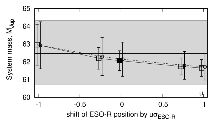
Figure 4: Median system mass with $1\,\sigma$ uncertainty ranges derived when applying an artificial shift to the ESO-R measurement. The shifts were applied in both coordinates by $u\sigma_{cat}$ toward ($u>0$) or away from ($u<0$) the model-predicted position, and the parameters $K_{\mathrm{ESO-R}}=0.57$ (open square boxes) or $K_{\mathrm{ESO-R}}=1$ (open circles) were used. The adopted value of $M_{tot}$ given in Table 5 is shown as a filled square. For comparison, the $1\,\sigma$ uncertainty range (gray area) and the median value (solid horizontal line) computed without the ESO-R measurements are shown.

If the ESO-R measurement is not used, we obtain slightly higher masses of $M_{tot}=(62.6\pm 1.8)M_{Jup}$, $M_{A}=(33.8\pm 0.9)M_{Jup}$, and $M_{B}=(28.8\pm 0.8)M_{Jup}$, which are still within the confidence intervals for the final solution in Table 5, but the uncertainties increased to 3% (Fig. 4).

A minor source of bias in the masses may stem from the seeing correction of the FORS2 measurements (Sect. 2.5), which partially relies on the external HST and GeMS data.

3.1.3 Comparison to Bedin et al. (2017) and Garcia et al. (2017)

Except for eccentricity, our parameter values agree with Bedin et al. (2017) within the error bars, but our estimates have smaller confidence intervals because we have access to a longer time span ($\sim$3.5 instead of 2 years). Our estimates also agree with the median parameter values obtained by Garcia et al. (2017) with the Markov chain Monte Calro (MCMC) analysis. Because of a larger volume of observations and improved reduction of FORS2 data, our confidence intervals are 2–10 fold narrower for most parameters, except for the orbital period $P,$ for which the interval 27.1–27.6 yr given by Garcia et al. (2017) is smaller than the interval 27.1–27.9 yr derived by us. In contrast to Garcia et al. (2017), we did not include radial velocity measurements in the fit, which may explain the slightly less well constrained period.

Figure 5: Motion of component B relative to A for the direct data fit (solid line) for all solutions expected within the 68.3% confidence interval (indicated by the space between the dashed lines), and the measured positions with FORS2 (open circles), HST (triangles), GeMS (squares), and ESO-R obtained in 1984 (the cross with error bars).

The inclination $i>90\degr$ that we obtained corresponds to the observed clockwise motion, whereas the value of $i<90\degr$ given by Bedin et al. (2017, Table 8) and Garcia et al. (2017) corresponds to a counterclockwise motion, assuming identical parameterization. In particular, we define $\omega$ as the argument of periastron for the barycentric orbit of the primary. The use of their orbital elements leads to equatorial positions with rearranged coordinate axes, that is, the computed RA is in fact Dec. From the definition of the Thiele-Innes parameters it follows that this inconsistency can be removed by changing $i$ to $180\degr-i$ and $\Omega$ to $270\degr-\Omega$. For instance, the parameters $i=79.21$ and $i=79.5\degr$, and $\Omega=130.3$ and $\Omega=130.12\degr$ given by Bedin et al. (2017, Table 8) and Garcia et al. (2017), respectively, are converted into $i=100.79$, $i=100.5\degr$, and $\Omega=139.7$, $\Omega=139.88\degr$ which matches our estimates well. The relative motion in the binary system is shown in Fig.5, which essentially agrees with Garcia et al. (2017) also in terms of the families of allowed orbital configurations.

Table 6: Radial relative velocity $V_{A}-V_{B}$ measured by CRIRES (Garcia et al. 2017) and the computed minimum/maximum values for our orbital solutions within the 68.3% confidence interval.

Date	$V_{A}-V_{B}$ (km/s)	min / max value (km/s)
2013.342	2.74$\pm$0.2	2.596 / 2.639
2014.333	1.94$\pm$0.2	1.915 / 1.957
2014.382	1.85$\pm$0.2	1.871 / 1.914

We also computed the radial velocity of component LUH16 A relative to B for all possible orbital solutions within the 68.3% confidence interval and compared these estimates (Table 6) with the corresponding CRIRES measurements presented by Garcia et al. (2017). These velocity measurements were not included in the fit because they do not increase the time span of the data set and have a small weight compared to the orbital astrometry. However, we confirmed that our solution is compatible and that the inclination is $0<i<180^{\degr}$. We found good agreement between our model-predicted minimum/maximum velocity and the data (Table 6) within the uncertainty range of the measurements.

We searched for a potential seeing dependence of the residuals $\Delta_{RA}$ in RA and $\Delta_{Dec}$ in Dec of the fit Eq.(7) that might be due to errors in the photocenter measurements caused by overlapping images. Errors of this kind are expected to occur along the line connecting the components of LUH 16. Therefore, projecting the residuals $\Delta_{RA}$ and $\Delta_{Dec}$ onto this line, we formed the equivalent residuals $\Delta_{||}$ , which we can correlate with $\varepsilon$. Because the binary system was oriented approximately at 45°relative to the coordinate axes, the projected residuals are found simply as $\Delta_{||}=(\Delta_{RA}-\Delta_{Dec})/\sqrt{2}$, with the positive values corresponding to the displacement of LUH 16 B toward A. Figure 6 shows that there is no significant dependence of $\Delta_{||}$ on seeing.

For comparison, we present $\Delta_{||}$ computed based on HST, GeMS, and astrometric measurements by Garcia et al. (2017, Table 2). With these data, we computed the orbital motion with Eq.(6), neglecting the DCR terms because these measurements are free from DCR, and obtained the residuals $\Delta_{RA}$ and $\Delta_{Dec}$ nearly equal to those shown by Garcia et al. (2017, Fig. 10). Then we formed the values $\Delta_{||}$ shown in Fig. 6 (open circles), which reveal a clear dependence on seeing. Their RMS of individual values is 1.2 mas, which significantly exceeds the value of 0.35 mas for our reduction. This comparison demonstrates the efficiency of our mitigation of seeing-dependent errors in the epoch-average positions using statistics of residuals $\Delta^{\prime}-\psi$ within individual frame series.

Figure 6: Residuals along the projected distance between components B and A for FORS2 measurements for our reduction (filled circles, $\sigma=0.35$ mas) and the reduction by Garcia et al. (2017) (open circles, $\sigma=1.2$ mas).

3.2 Deriving the mass ratio and astrometric parameters

By fitting all HST, FORS2, and GeMS observations with the model for the barycenter motion of Eq.(8) in its simple form with $\Delta=0$ and $\varepsilon_{0}$ derived in Sect. 3.1, we derived the first solution (left column of Table 7), yielding $q=0.865$. This value of $q$ gives the smallest rms of 0.359 mas (0.352 and 0.366 mas along RA and Dec) for the residuals of all observed and model positions shown in the lower panel of Fig.7 in RA.

Table 7: Barycenter parameters for two versions of model Eq.(8), without ($\Delta=0$), and with separate offsets ($\Delta\neq 0$) in FORS2 and HST measurements, and the solution by Garcia et al. (2017). Zero-points $x_{c}$, $y_{c}$ are derived with reference to $\alpha=162.3107300\degr$, $\delta=-53.3181500\degr$, ICRF, epoch J2015.0, and the zero time is $t_{0}=56500$ MJD. The precision $\sigma_{\mathrm{fit}}$ refers to the least-squares fit of the linear Eq.-s (8) with fixed $q,$ while $\sigma_{\mathrm{stat}}$ takes into account statistical variations of $q$ within $\pm 0.0024$.

parameter	no offset ($\Delta=0$)		separate offset			Garcia 2017
	value $\pm\sigma_{\mathrm{fit}}$		value $\pm\sigma_{\mathrm{fit}}$		$\sigma_{\mathrm{stat}}$	value $\pm\sigma$
$q$	0.8650	$\pm$ 0.0024	0.8519	$\pm$ 0.0024	-	0.82	$\pm$ 0.03
$x_{c}$ (mas)	24.371	$\pm$ 0.066	28.338	$\pm$ 0.063	1.332	-
$y_{c}$ (mas)	333.713	$\pm$ 0.097	330.146	$\pm$ 0.104	1.190	-
$\mu_{x}$ (mas/yr)	-2759.709	$\pm$ 0.045	-2760.884	$\pm$ 0.077	0.384	-2762	$\pm$ 2.5
$\mu_{y}$ (mas/yr)	353.208	$\pm$ 0.053	354.753	$\pm$ 0.075	0.481	358	$\pm$ 3.5
$\rho$ (mas)	37.582	$\pm$ 6.64	39.129	$\pm$ 6.29	6.29	38.06	$\pm$ 8
$\rho_{A}$ (mas)	38.192	$\pm$ 9.31	39.802	$\pm$ 7.99	8.35	-
$\rho_{B}$ (mas)	36.877	$\pm$ 11.58	38.339	$\pm$ 9.94	10.40	-
$d$ (mas)	-51.314	$\pm$ 5.64	-52.199	$\pm$ 5.16	5.40	-48.73	$\pm$ 7
$d_{A}$ (mas)	-50.897	$\pm$ 7.66	-51.554	$\pm$ 6.55	6.80	-
$d_{B}$ (mas)	-51.796	$\pm$ 9.53	-52.956	$\pm$ 8.15	8.51	-
$\varpi$(mas)	501.165	$\pm$ 0.055	501.215	$\pm$ 0.053	0.061	501.01	$\pm$ 0.51
$\Delta_{x}$ (mas)	0		-0.095	$\pm$ 0.081	0.169	-
$\Delta_{y}$ (mas)	0		+0.303	$\pm$ 0.080	0.197	-
rms (mas)	0.359		0.340		-

Figure 7: Residuals between the FORS2 (open circles), HST (triangles), and GeMS (filled circles) measured barycenter position of LUH 16 and the model of Eq. (8). The middle and upper panels are obtained assuming that offsets $\Delta$ are different for each telescope, while the lower panel shows the residuals in RA for the standard model of Eq. (8) with no offset ($\Delta=0$). The $\sigma$ values refer to the average rms of residuals in RA and Dec for both HST and FORS2.

To set the uncertainty limits for $q$, we used the Monte Carlo method, creating random samples of FORS2 and HST measured positions, and processed them with different values of $q$. For each sample, we determined the best $q$ value as that which corresponds to the minimum rms of the positional residuals. The scatter of these values around the average is characterized by the 1 $\sigma$ interval of 0.0024 and corresponds to the statistical uncertainty of the $q$ value determination. With $q$ fixed to 0.865, Eq.-s (8) is solved by the least-squares fit as a linear system of equations, and the uncertainty $\sigma_{\mathrm{fit}}$ of the parameters derived thus is given in Table 7.

Eq. (8), however, is a nonlinear system if $q$ is considered as a free model parameter. The direct solution of this expanded model is same as the solution of the linear model with $q=0.865$, but the uncertainties of parameters are quite different. They were estimated by the above Monte Carlo simulation when, together with $q$, for each random sample we also derived all parameters of the model of Eq.(8). Thus, for each parameter we obtained a set of solutions that corresponds to the expected statistical variations of $q$. Thus computed 1 $\sigma$ deviations $\sigma_{\mathrm{stat}}$ for each parameter are given in Table 7. Unlike the linear model, some parameters of the expanded model (e.g., $x_{c}$ and $\mu_{x}$) are highly correlated, which is indicated by the inequality $\sigma_{\mathrm{stat}}\gg\sigma_{\mathrm{fit}}$. In parameter space, the values of these parameters are concentrated along a line with a small scatter corresponding to $\sigma_{\mathrm{fit}}$.

The residuals for GeMS shown in Fig. 7 are qualitatively equal to those obtained by Garcia et al. (2017, Fig.12). In comparison to FORS2 and HST residuals, they are more scattered, possibly because of insufficiently precise transformation into ICRF. Because of a large scatter $\sigma$, the barycenter parameters of LUH 16 and the RMS of the residuals were computed with zero weights for the GeMS data. However, we expect that the zero-point errors do not affect the distances between components A and B, and the scatter in the distances measured with GeMS and shown in Fig.3 are indeed much smaller than those in Fig.7. Indirectly, these features support our assumption on the origin of $\Delta$ in Sect. 2.6, and that it is instrument dependent and should be included in the model of Eq.(6).

The large uncertainties of the chromatic parameters $\rho$ and $d$ in Table 7 are due to the large and expected correlation of about -0.9996, which means that the DCR displacement correction by the LADC is modeled by Eq. 1 with an uncertainty smaller than 0.1 mas.

The high precision in the $x_{c}$, $y_{c}$ offset determination ($\pm 0.066$ and $\pm 0.097$ mas), which is much better than the uncertainty of the transformation Eq.(5) into the ICRF of about 0.5 mas, motivated us to try out a model function with different offsets $\Delta(\mathrm{HST})$ for HST and $\Delta(\mathrm{FORS2})$ for FORS2. This produced the second solution with better rms of 0.340 mas achieved at $q=0.8519$ (Table 7). In this model we cannot distinguish the offsets, however, and instead obtained $x_{c}+\Delta_{x}(\mathrm{HST})=28.433\pm 0.162$, $x_{c}+\Delta_{x}(\mathrm{FORS2})=28.243\pm 0.063$, $y_{c}+\Delta_{y}(\mathrm{HST})=329.843\pm 0.159$ and $y_{c}+\Delta_{y}(\mathrm{FORS2})=330.449\pm 0.104$ mas. Each of these sums corresponds to the zero-point of the barycenter in the FORS2 or HST system, but they are significantly, about 3–4 mas, different from those derived for the first solution. We verified that this is due to the difference in $q$ but not because different offsets $\Delta$ were introduced.

The difference between the FORS2 and HST zero-points $\Delta_{x}(\mathrm{FORS2})-\Delta_{x}(\mathrm{HST})=-0.190$ and $\Delta_{y}(\mathrm{FORS2})-\Delta_{y}(\mathrm{HST})=+0.606$ mas is comparable to the uncertainty in the zero-points of the transformation into the ICRF, giving a potential explanation for the discrepancy. To confirm this, we derived the corresponding values for a transformation (Sect. 2.6) using Gaia DR1 and obtained significantly larger differences $\Delta_{x}(\mathrm{FORS2})-\Delta_{x}(\mathrm{HST})=-0.816$ in RA and $\Delta_{y}(\mathrm{FORS2})-\Delta_{y}(\mathrm{HST})=+1.199$ mas in Dec. This demonstrates the difference between Gaia DR1 and DR2 and supports our assumption on the origin of this discrepancy.

Fig. 7 shows the difference between the two solutions: with use of common $x_{c}$, $y_{c}$ (bottom panel) and offsets different for each data set (middle panel), which we illustrate here in RA. Visually, the gain in overall RMS is small ($\sigma$ decreased from 0.36 to 0.33 mas in RA), but for the subset of FORS2 residuals, the improvement is more significant (0.31 mas versus 0.24 mas). We applied the F-test of additional parameters to find that the improvement is statistically significant. With all FORS2 and HST measurements along RA and Dec, we derived $F\approx 10$ with 2 and 114 degrees of freedom, which means that the simpler model is true with a probability $<10^{-4}$.

Finally, we converted the barycenter parameters obtained with separate offsets in Table 7 into the absolute system with the correction terms determined in Sect. 2.6.2. We obtained absolute proper motions and parallaxes of $\mu_{x}=-2767.502\pm 0.147$ mas/yr, $\mu_{y}=356.856\pm 0.150$ mas/yr, and $\varpi_{\mathrm{abs}}=501.557\pm 0.082$ mas.

3.3 Corrected FORS2 positions

Now we can apply corrections to the FORS2 measurements to remove the difference in offsets $\Delta$. Since we have no handle on the proportion with which the discrepancy occurs, the errors were assumed equal in magnitude but opposite in sign, that is, $\Delta(\mathrm{FORS2})=-\Delta(\mathrm{HST})=\Delta$. The barycenter zero-point $x_{c}$, $y_{c}$ and the offsets $\Delta$ to the system of equatorial positions at the location of LUH 16 on the CCD obtained in this assumption are given in Table 7. The corrections $x(\mathrm{FORS2})-\Delta_{x}$, $y(\mathrm{FORS2})-\Delta_{y}$, $x(\mathrm{HST})+\Delta_{x}$, $y(\mathrm{HST})+\Delta_{y}$ reduce these two data sets of positions to a system anchored at the ICRF. In Table 3 we give the positions

$$\begin{array}[]{@{}ll}x^{*}_{A}=&x_{A}+\rho_{A}f_{1,x}+d_{A}f_{2,x}+k^{x}_{1,A}\varepsilon_{0}-\Delta_{x}\\ y^{*}_{A}=&y_{A}-\rho_{A}f_{1,y}-d_{A}f_{2,y}+k^{y}_{1,A}\varepsilon_{0}-\Delta_{y}\\ \end{array}$$ (9)

corrected also for DCR and other calibrations, where the expressions for LUH 16 B are similar.

4 Conclusion and discussion

We presented an improved reduction of the FORS2 astrometric measurements of the LUH 16 binary and showed that they are consistent with the HST and GeMS positions in the literature. In our previous reduction (Sahlmann & Lazorenko 2015), the positions of LUH 16 were linked to the ICRF using USNO-B, and as noted by Bedin et al. (2017), are inconsistent with the HST measurements at a level of 10–20 mas. This was due to a flawed transformation into the ICRF that used stars in both chips of FORS2. Before Gaia DR1, this effect could not be diagnosed and lead to a significant bias in RA, Dec of about $\pm$50 mas (Lazorenko & Sahlmann 2017). It had only a negligible effect on the relative positions of the LUH 16 components via the pixel scale and rotation of the coordinate axes, however. The main reason for the inconsistency noted by Bedin et al. (2017) was the incorrect transformation into the ICRF with Eq.(5), where as the argument of functions $F_{n}$ we used the positions of LUH 16 $\bar{x}$, $\bar{y}$ extrapolated to the USNO-B epoch J2000.0 instead of using the positions at the actual epochs.

Gaia DR2 provides the reference frame for determining absolute proper motions and parallaxes. However, we argue that very large ground-based telescopes provide us with competitive differential astrometry for faint 16–21 mag stars. In the LUH 16 field analyzed in this paper, the relative proper motions and parallaxes were determined with FORS2 with an average precision of 0.18 mas/yr and 0.13 mas, respectively, for 16–21 mag stars in common with DR2. In spite of the short one-year duration of FORS2 observations, this precision is about twice better than the corresponding values 0.48 mas/yr and 0.31 mas in the DR2 catalog. The good astrometric performance of FORS2 is due to the higher signal-to-noise ratio in the position estimation.

We refined the individual dynamical masses of LUH 16 to $33.5\pm 0.3\,M_{Jup}$ (component A) and $28.6\pm 0.3\,M_{Jup}$ (component B), which corresponds to a relative precision of $\sim$1% and is three to four times more precise than the estimates of Garcia et al. (2017). We found that a minor bias with $1\sigma$ of the ESO-R resolved astrometry based on a 1984 photographic plate leads to a change in the dynamical masses that does not exceed the random error of our determination. The exact characterization of any residual bias in mass will be resolved in the future when the high-precision astrometry will cover a larger portion of the orbit.

Because of the importance of LUH 16 as an extremely well-studied system of nearby brown dwarfs, the refinement of the parallax, orbital, and dynamical mass parameters will continue, with the purpose of increasing the knowledge of the physical parameters of the system. We expect that the astrometric data set presented here will contribute significantly to this process.