Improving Abstraction in Text Summarization

Abstract

Abstractive text summarization aims to shorten long text documents into a human readable form that contains the most important facts from the original document. However, the level of actual abstraction as measured by novel phrases that do not appear in the source document remains low in existing approaches. We propose two techniques to improve the level of abstraction of generated summaries. First, we decompose the decoder into a contextual network that retrieves relevant parts of the source document, and a pretrained language model that incorporates prior knowledge about language generation. Second, we propose a novelty metric that is optimized directly through policy learning to encourage the generation of novel phrases. Our model achieves results comparable to state-of-the-art models, as determined by ROUGE scores and human evaluations, while achieving a significantly higher level of abstraction as measured by $n$-gram overlap with the source document.

1 Introduction

Article

(cnn) to allay possible concerns, boston prosecutors released video friday of the shooting of a police officer last month that

resulted in the killing of the gunman. the officer wounded, john moynihan, is white. angelo west, the gunman shot to death

by officers, was black. after the shooting, community leaders in the predominantly african-american neighborhood of (…)

Human-written summary

boston police officer john moynihan is released from the hospital. video shows that the man later shot dead by police in

boston opened fire first. moynihan was shot in the face during a traffic stop.

Generated summary (See et al., 2017)

boston prosecutors released video friday of the shooting of a police officer last month. the gunman shot to death by officers,

was black. one said the officers were forced to return fire. he was placed in a medically induced coma at a boston hospital.

Generated summary (Liu et al., 2018)

boston prosecutors released video of the shooting of a police officer last month. the shooting occurred in the wake of the

boston marathon bombing. the video shows west sprang out and fired a shot with a pistol at officer’s face.

Our summary (ML+RL ROUGE+Novel, with LM)

new: boston police release video of shooting of officer , john moynihan. new: angelo west had several prior gun convictions,

police say. boston police officer john moynihan, 34, survived with a bullet wound. he was in a medically induced coma at

a boston hospital, a police officer says.

Table 1: Summaries generated by different models for the same CNN/Daily Mail article. The highlighted spans indicate phrases of 3 tokens or more that are copied word-by-word from the original article.

Text summarization concerns the task of compressing a long sequence of text into a more concise form. The two most common approaches to summarization are extractive (Dorr et al., 2003; Nallapati et al., 2017), where the model extracts salient parts of the source document, and abstractive (Paulus et al., 2017; See et al., 2017), where the model not only extracts but also concisely paraphrases the important parts of the document via generation. We focus on developing a summarization model that produces an increased level of abstraction. That is, the model produces concise summaries without only copying long passages from the source document.

A high quality summary is shorter than the original document, conveys only the most important and no extraneous information, and is semantically and syntactically correct. Because it is difficult to gauge the correctness of the summary, evaluation metrics for summarization models use word overlap with the ground-truth summary in the form of ROUGE (Lin, 2004) scores. However, word overlap metrics do not capture the abstractive nature of high quality human-written summaries: the use of paraphrases with words that do not necessarily appear in the source document.

The state-of-the-art abstractive text summarization models have high word overlap performance, however they tend to copy long passages of the source document directly into the summary, thereby producing summaries that are not abstractive (See et al., 2017).

We propose two general extensions to summarization models that improve the level of abstraction of the summary while preserving word overlap with the ground-truth summary. Our first contribution decouples the extraction and generation responsibilities of the decoder by factoring it into a contextual network and a language model. The contextual network has the sole responsibility of extracting and compacting the source document whereas the language model is responsible for the generation of concise paraphrases. Our second contribution is a mixed objective that jointly optimizes the $n$-gram overlap with the ground-truth summary while encouraging abstraction. This is done by combining maximum likelihood estimation with policy gradient. We reward the policy with the ROUGE metric, which measures word overlap with the ground-truth summary, as well as a novel abstraction reward that encourages the generation of words not in the source document.

We demonstrate the effectiveness of our contributions on a encoder-decoder summarization model. Our model obtains state-of-the-art ROUGE-L scores, and ROUGE-1 and ROUGE-2 performance comparable to state-of-the-art methods on the CNN/DailyMail dataset. Moreover, we significantly outperform all previous abstractive approaches in our abstraction metrics. Table 1 shows a comparison of summaries generated by our model and previous abstractive models, showing less copying and more abstraction in our model.

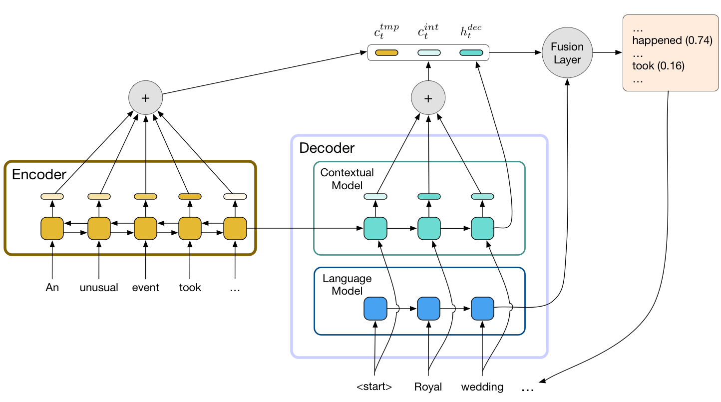
Figure 1: The network architecture with the decoder factorized into separate contextual and language models. The reference vector, composed of context vectors $c^{tmp}_{t}$, $c^{int}_{t}$, and the hidden state of the contextual model $h^{dec}_{t}$, is fused with the hidden state of the language model and then used to compute the distribution over the output vocabulary.

2 Model

2.1 Base Model and Training Objective

The base model follows the encoder-decoder architecture with temporal attention and intra-attention proposed by Paulus et al. (2017). Let $E\in{\mathbb{R}}^{n\times d^{\rm{emb}}}$ denote the matrix of $d^{\rm{emb}}$ dimensional word embeddings of the $n$ words in the source document. The encoding of the source document $h^{\rm{enc}}$ is computed via a bidirectional LSTM (Hochreiter and Schmidhuber, 1997) whose output has dimension $d^{\rm{hid}}$.

$$h^{\rm{enc}}={\rm{BiLSTM}}\left(E\right)\in{\mathbb{R}}^{n\times d^{\rm{hid}}}$$ (1)

The decoder uses temporal attention over the encoded sequence that penalizes input tokens that previously had high attention scores. Let $h^{\rm{dec}}_{t}$ denote the decoder state at time $t$. The temporal attention context at time $t$, $c^{\rm{tmp}}_{t}$, is computed as

$$s^{\rm{tmp}}_{ti} = \left(h^{\rm{dec}}_{t}\right)^{\intercal}W^{\rm{tmp}}h^{\rm{enc}}_{i}\in{\mathbb{R}}$$ (2)

$$q^{\rm{tmp}}_{ti} = \frac{\exp(s^{\rm{tmp}}_{ti})}{\sum^{t-1}_{j=1}\exp(s^{\rm{tmp}}_{ji})}\in{\mathbb{R}}$$ (3)

$$\alpha^{\rm{tmp}}_{ti} = \frac{q^{\rm{tmp}}_{ti}}{\sum^{n}_{j=1}q^{\rm{tmp}}_{tj}}\in{\mathbb{R}}$$ (4)

$$c^{\rm{tmp}}_{t} = \sum^{n}_{i=1}\alpha^{\rm{tmp}}_{ti}h^{\rm{enc}}_{i}\in{\mathbb{R}}^{d^{\rm{hid}}}$$ (5)

where we set $q^{\rm{tmp}}_{ti}$ to $\exp(s^{\rm{tmp}}_{ti})$ for $t=1$.

The decoder also attends to its previous states via intra-attention over the decoded sequence. The intra-attention context at time $t$, $c^{\rm{int}}_{t}$, is computed as

$$s^{\rm{int}}_{ti} = \left(h^{dec}_{t}\right)^{\intercal}W^{\rm{int}}h^{\rm{dec}}_{i}\in{\mathbb{R}}$$ (6)

$$c^{\rm{int}}_{t} = \sum^{t-1}_{i=1}\left(\frac{s^{\rm{int}}_{ti}}{\sum^{n}_{j=1}s^{\rm{int}}_{tj}}\right)h^{\rm{dec}}_{i}\in{\mathbb{R}}^{d^{\rm{hid}}}$$ (7)

The decoder generates tokens by interpolating between selecting words from the source document via a pointer network as well as selecting words from a fixed output vocabulary. Let $z_{t}$ denote the ground-truth label as to whether the $t$th output word should be generated by the selecting from the output vocabulary as opposed to from the source document. We compute $p(z_{t})$, the probability that the decoder generates from the output vocabulary, as

$$r_{t} =[h^{\rm{dec}}_{t};c^{\rm{tmp}}_{t};c^{\rm{int}}_{t}]\in{\mathbb{R}}^{3d^{\rm{hid}}}$$ (8)

$$p(z_{t}) ={\rm{sigmoid}}(W^{\rm{z}}r_{t}+b^{\rm{z}})\in{\mathbb{R}}$$ (9)

The probability of selecting the word $y_{t}$ from a fixed vocabulary at time step $t$ is defined as

$$p^{\rm{gen}}(y_{t})={\rm{softmax}}\left(W^{\rm{gen}}r_{t}+b^{\rm{gen}}\right)$$ (10)

We set $p^{\rm{cp}}(y_{t})$, the probability of copying the word $y_{t}$ from the source document, to the temporal attention distribution $\alpha^{\rm{tmp}}_{t}$. The joint probability of using the generator and generating the word $y_{t}$ at time step $t$, $p(z_{t},y_{t})$, is then

$$p(z_{t},y_{t})=p(y_{t}\mid z_{t})p(z_{t})$$ (11)

the likelihood of which is

$$\begin{split}&\log p(z_{t},y_{t})=\log p(y_{t}\mid z_{t})+\log p(z_{t})\\ &=z_{t}\log p^{\rm{gen}}(y_{t})+(1-z_{t})\log p^{\rm{cp}}(y_{t})\\ &\text{\quad}+z_{t}\log p(z_{t})+\left(1-z_{t}\right)\log\left(1-p\left(z_{t}\right)\right)\\ &=z_{t}\left(\log p^{\rm{gen}}(y_{t})+\log p(z_{t})\right)\\ &\text{\quad}+(1-z_{t})\left(\log p^{\rm{cp}}(y_{t})+\log\left(1-p\left(z_{t}\right)\right)\right)\end{split}$$ (12)

The objective function combines maximum likelihood estimation with policy learning. Let $m$ denote the length of the ground-truth summary, The maximum likelihood loss $L^{\rm{ml}}$ is computed as

$$L^{\rm{ml}}=-\sum^{m}_{t=1}\log p(z_{t},y_{t})$$ (13)

Policy learning uses ROUGE-L as its reward function and a self-critical baseline using the greedy decoding policy (Rennie et al., 2016). Let $y^{\rm{sam}}$ denote the summary obtained by sampling from the current policy $p$, $y^{\rm{gre}}$ and $z^{\rm{gre}}$ the summary and generator choice obtained by greedily choosing from $p(z_{t},y_{t})$, $R(y)$ the ROUGE-L score of the summary $y$, and $\Theta$ the model parameters. The policy learning loss is

$$\hat{R} = R\left(y^{\rm{sam}}\right)-R\left(y^{\rm{gre}}\right)$$ (14)

$$L^{\rm{pg}} = -\mathbb{E}_{\begin{subarray}{c}z^{\rm{sam}}~{}\sim p(z),\\ y^{\rm{sam}}~{}\sim p(y|z)\end{subarray}}[\hat{R}]$$ (15)

where we use greedy predictions by the model according to eq. (13) as a baseline for variance reduction. The policy gradient, as per Schulman et al. (2015), is

$$\nabla_{\Theta}L^{\rm{pg}}\approx-\hat{R}\sum_{t=1}^{m}\nabla_{\Theta}\log p\left(z^{\rm{sam}}_{t},y^{\rm{sam}}_{t}\right)$$ (16)

The final loss is a mixture between the maximum likelihood loss and the policy learning loss, weighted by a hyperparameter $\gamma$.

$$L=(1-\gamma)L^{\rm{ml}}+\gamma L^{\rm{pg}}$$ (17)

2.2 Language Model Fusion

The decoder is an essential component of the base model. Given the source document and the previously generated summary tokens, the decoder both extracts relevant parts of the source document through the pointer network as well as composes paraphrases from the fixed vocabulary. We decouple these two responsibilities by augmenting the decoder with an external language model. The language model assumes responsibility of generating from the fixed vocabulary, and allows the decoder to focus on attention and extraction. This decomposition has the added benefit of easily incorporating external knowledge about fluency or domain specific styles via pre-training the language model on a large scale text corpora.

The architecture of our language model is based on Merity et al. (2018). We use a 3-layer unidirectional LSTM with weight-dropped LSTM units.

Let $e_{t}$ denote the embedding of the word generated during time step $t$. The hidden state of the language model at the $l$-th layer is

$$h^{\rm{lm}}_{l,t}={\rm{LSTM}}^{\rm{lm}}_{3}\left(e_{t-1},h^{\rm{lm}}_{l,t-1}\right)$$ (18)

At each time step $t$, we combine the hidden state of the last language model LSTM layer, $h^{\rm{lm}}_{3,t}$, with $r_{t}$ defined in eq. (8) in a fashion similar to Sriram et al. (2017). Let $\odot$ denote element-wise multiplication. We use a gating function whose output $g_{t}$ filters the content of the language model hidden state.

$$f_{t} = {\rm{sigmoid}}\left(W^{\rm{lm}}[r_{t};h^{\rm{lm}}_{3,t}]+b^{\rm{lm}}\right)$$ (19)

$$g_{t} = W^{\rm{fuse}}([r_{t};g_{t}\odot h^{\rm{lm}}_{3,t}])+b^{\rm{fuse}}$$ (20)

$$h^{\rm{fuse}}_{t} = {\rm{ReLU}}\left(g_{t}\right)$$ (21)

We then replace the output distribution of the language model $p^{\rm{gen}}\left(y_{t}\right)$ in eq. 10 with

$$p^{\rm{gen}}\left(y_{t}\right)={\rm{softmax}}\left(W^{\rm{gen}}h^{\rm{fuse}}_{t}+b^{\rm{gen}}\right)$$ (22)

2.3 Abstractive Reward

In order to produce an abstractive summary, the model cannot exclusively copy from the source document. In particular, the model needs to parse large chunks of the source document and create concise summaries using phrases not in the source document. To encourage this behavior, we propose a novelty metric that promotes the generation of novel words.

We define a novel phrase in the summary as one that is not in the source document. Let ${\rm{ng}}\left(x,n\right)$ denote the function that computes the set of unique $n$-grams in a document $x$, $x^{\rm{gen}}$ the generated summary, $x^{\rm{src}}$ the source document, and $\left\lVert s\right\rVert$ the number of words in $s$. The unnormalized novelty metric $N$ is defined as the fraction of unique $n$-grams in the summary that are novel.

$$N\left(x^{\rm{gen}},n\right)=\frac{\left\lVert{\rm{ng}}\left(x^{\rm{gen}},n\right)-{\rm{ng}}\left(x^{\rm{src}},n\right)\right\rVert}{\left\lVert{\rm{ng}}\left(x^{\rm{gen}},n\right)\right\rVert}$$ (23)

To prevent the model for receiving high novelty rewards by outputting very short summaries, we normalize the metric by the length ratio of the generated and ground-truth summaries. Let $x^{\rm{gt}}$ denote the ground-truth summary. We define the novelty metric as

$$R^{\rm{nov}}\left(x^{\rm{gen}},n\right)=N\left(x^{\rm{gen}},n\right)\frac{\left\lVert x^{\rm{gen}}\right\rVert}{\left\lVert x^{\rm{gt}}\right\rVert}$$ (24)

We incorporate the novelty metric as a reward into the policy gradient objective in eq. (15), alongside the original ROUGE-L metric. In doing so, we encourage the model to generate summaries that both overlap with human written ground-truth summaries as well as incorporate novel words not in the source document:

$$R\left(y\right)=\lambda^{\rm{rou}}R^{\rm{rou}}\left(y^{\rm{sam}}\right)+\lambda^{\rm{nov}}R^{\rm{nov}}\left(y^{\rm{sam}}\right)$$ (25)

where $\lambda^{\rm{rou}}$ and $\lambda^{\rm{nov}}$ are hyperparameters that control the weighting of each reward.

3 Experiments

3.1 Datasets

We train our model on the CNN/Daily Mail dataset (Hermann et al., 2015; Nallapati et al., 2016). Previous works on abstractive summarization either use an anonymized version of this dataset or the original article and summary texts. Due to these different formats, it is difficult to compare the overall ROUGE scores and performance between each version. In order to compare against previous results, we train and evaluate on both versions of this dataset. For the anonymized version, we follow the pre-processing steps described in Nallapati et al. (2016), and the pre-processing steps of See et al. (2017) for the the full-text version.

Model	R-1	R-2	R-L	NN-1	NN-2	NN-3	NN-4
anonymized
Ground-truth summaries	-	-	-	14.40	52.07	71.63	80.84
ML+RL, intra-attn (Paulus et al., 2017)	39.87	15.82	36.9	1.04	10.86	21.53	29.27
ML+RL ROUGE+Novel, with LM (ours)	40.02	15.53	37.44	3.54	21.91	37.48	47.13
full-text
Ground-truth summaries	-	-	-	13.55	49.97	70.32	80.02
Pointer-gen + coverage (See et al., 2017)	39.53	17.28	36.38	0.07	2.24	6.03	9.72
SumGAN (Liu et al., 2018)	39.92	17.65	36.71	0.22	3.15	7.68	11.84
RSal (Pasunuru and Bansal, 2018)	40.36	17.97	37.00	-	2.37	6.00	9.50
RSal+Ent RL (Pasunuru and Bansal, 2018)	40.43	18.00	37.10	-	-	-	-
ML+RL ROUGE+Novel, with LM (ours)	40.19	17.38	37.52	3.25	17.21	30.46	39.47

Table 2: Comparison of ROUGE (R-) and novel $n$-gram (NN-) test results for our model and other abstractive summarization models on the CNN/Daily Mail dataset.

We use named entities and the source document to supervise the model regarding when to use the pointer and when to use the generator (e.g. $z_{t}$ in eq. (13). Namely, during training, we teach the model to point from the source document if the word in the ground-truth summary is a named entity, an out-of-vocabulary word, or a numerical value that is in the source document. We obtain the list of named entities from Hermann et al. (2015).

3.2 Language Models

For each dataset version, we train a language model consisting of a 400-dimensional word embedding layer and a 3-layer LSTM with each layer having a hidden size of 800 dimensions, except the last input layer which has an output size of 400. The final decoding layer shares weights with the embedding layer (Inan et al., 2017; Press and Wolf, 2016). We also use DropConnect (Wan et al., 2013) in the hidden-to-hidden connections, as well as the non-monotonically triggered asynchronous gradient descent optimizer from Merity et al. (2018).

We train this language model on the CNN/Daily Mail ground-truth summaries only, following the same training, validation, and test splits as our main experiments.

3.3 Training details

The two LSTMs of our bidirectional encoder are 200-dimensional, and out decoder LSTM is 400-dimensional. We restrict the input vocabulary for the embedding matrix to 150,000 tokens, and the output decoding layer to 50,000 tokens. We limit the size of input articles to the first 400 tokens, and the summaries to 100 tokens. We use scheduled sampling (Bengio et al., 2015) with a probability of 0.25 when calculating the maximum-likelihood training loss. We also set $n=3$ when computing our novelty reward $R^{nov}(x_{gen},n)$. For our final training loss using reinforcement learning, we set $\gamma=0.9984$, $\lambda^{rou}=0.9$, and $\lambda^{nov}=0.1$. Finally, we use the trigram repetition avoidance heuristic defined by Paulus et al. (2017) during beam search decoding to ensure that the model does not output twice the same trigram in a given summary, reducing the amount of repetitions.

3.4 Novelty baseline

We also create a novelty baseline by taking the outputs of our base model, without RL training and without the language model, and inserting random words not present in the article after each summary token with a probability $r=0.0005$. This baseline will intuitively have a higher percentage of novel $n$-grams than our base model outputs while being very similar to these original outputs, hence keeping the ROUGE score difference relatively small.

4 Results

4.1 Quantitative analysis

We obtain a validation and test perplexity of 65.80 and 66.61 respectively on the anonymized dataset, and 81.13 and 82.98 on the full-text dataset with the language models described in Section 3.2.

The ROUGE scores and novelty scores of our final summarization model on both versions of the CNN/Daily Mail dataset are shown in Table 2. We report the ROUGE-1, ROUGE-2, and ROUGE-L F-scores as well as the percentage of novel $n$-grams, marked NN-$n$, in the generated summaries, with $n$ from 1 to 4. Results are omitted in cases where they have not been made available by previous authors. We also include the novel $n$-gram scores for the ground-truth summaries as a comparison to indicate the level of abstraction of human written summaries.

Even though our model outputs significantly fewer novel $n$-grams than human written summaries, it has a much higher percentage of novel $n$-grams than all the previous abstractive approaches. It also achieves state-of-the-art ROUGE-L performance on both dataset versions, and obtains ROUGE-1 and ROUGE-2 scores close to state-of-the-art results.

4.2 Ablation study

Model	R-1	R-2	R-L	NN-1	NN-2	NN-3	NN-4
ML	39.21	15.47	36.27	2.47	14.1	25.35	33.46
ML with nov. baseline, $r=0.0005$	38.62	15.06	35.75	3.12	14.96	26.45	34.76
ML with LM	39.43	15.68	36.45	3.36	15.25	26.06	33.57
ML+RL ROUGE	41.02	16.62	38.13	2.2	12.88	24.16	32.5
ML+RL ROUGE, with LM	41.06	16.84	38.01	2.06	10.9	19.78	26.33
ML+RL ROUGE+Novel	40.61	15.84	38.06	3.19	22.79	39.9	50.61
ML+RL ROUGE+Novel, with LM	40.72	15.95	38.14	3.49	21.89	37.31	46.85

Table 3: Ablation study on the validation set of the anonymized CNN/Daily Mail dataset.

In order to evaluate the relative impact of each of our individual contributions, we run ablation studies comparing our model ablations against each other and against the novelty baseline. The results of these different models on the validation set of the anonymized CNN/Daily Mail dataset are shown in Table 3. Results show that our base model trained with the maximum-likelihood loss only and using the language model in the decoder (ML, with LM) has higher ROUGE scores, novel unigrams, and novel bigrams scores than our base model without the language model (ML). ML with LM also beats the novelty baseline for these metrics. When training these models with reinforcement learning using the ROUGE reward (ML+RL ROUGE and ML+RL ROUGE with LM), the model with language model obtains higher ROUGE-1 and ROUGE-2 scores. However, it also loses its novel unigrams and bigrams advantage. Finally, using the mixed ROUGE and novelty rewards (ML+RL ROUGE+Novel) produces both higher ROUGE scores and more novel unigrams with the language model than without it. This indicates that the combination of the language model in the decoder and the novelty reward during training makes our model produce more novel unigrams while maintaining high ROUGE scores.

4.3 ROUGE vs novelty trade-off

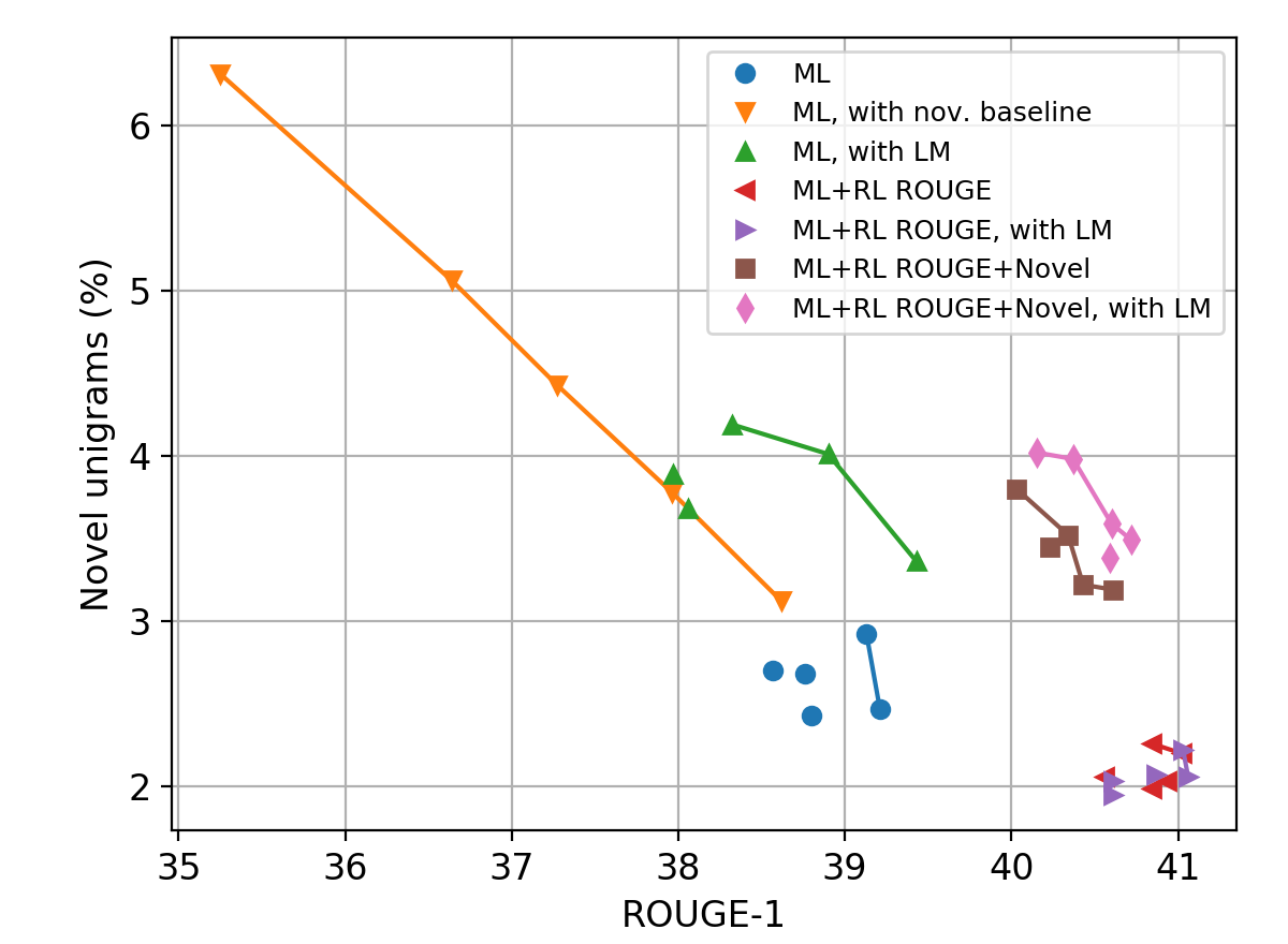
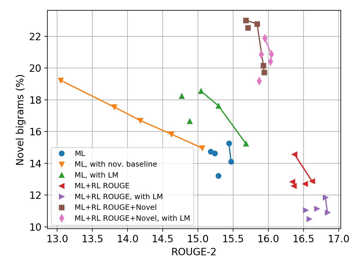
Figure 2: ROUGE and novel $n$-grams results on the anonymized validation set for different runs of each model type. Lines indicates the Pareto frontier for each model type.

Model	Readability	Relevance
Pointer-gen + coverage (See et al., 2017)	6.76 $\pm$ 0.17	6.73 $\pm$ 0.17
SumGAN (Liu et al., 2018)	6.79 $\pm$ 0.16	6.74 $\pm$ 0.17
ML+RL ROUGE+Novel, with LM	6.35 $\pm$ 0.19	6.63 $\pm$ 0.18

Table 4: Mean and confidence interval at 95% of human evaluation scores on the full-text test outputs. Individual summaries are rated from 1 to 10, a higher score indicating higher quality, for readability and relevance separately.

In order to understand the correlation between ROUGE and novel $n$-gram scores across different architectures, and to find the model type that gives the best trade-off between each of these metrics, we plot the ROUGE-1 and novel unigram scores for the five best iterations of each model type on the anonymized dataset, as well as the ROUGE-2 and novel bigram scores on a separate plot. We also include the novelty baseline described in Section 4.2 for values of $r$ between 0.005 and 0.035. For each model type, we indicate the Pareto frontier by a line plot (Ben-Tal, 1980), illustrating which models of a given type give the best combination of ROUGE and novelty scores. These plots are shown in Figure 2.

These plots show that there exist an inverse correlation between ROUGE and novelty scores in all model types, illustrating the challenge of choosing a model that performs well in both. Given that, our final model (ML+RL ROUGE+Novel, with LM) provides the best trade-off of ROUGE-1 scores compared to novel unigrams, indicated by the higher Pareto frontier in the first plot. Similarly, our final model gives one of the best trade-offs of ROUGE-2 scores to novel bigrams, even though the same model without LM produces more novel bigrams with a lower ROUGE-2 score.

4.4 Qualitative evaluation

In order to ensure the quality of our model outputs, we ask 5 human evaluators to rate 100 randomly selected full-text test summaries, giving them two scores from 1 to 10 respectively for readability and relevance given the original article. We also include the full-text test outputs from  See et al. (2017) and  Liu et al. (2018) for comparison. Evaluators are shown different summaries corresponding to the same article side by side without being told which models have generated them. The mean score and confidence interval at 95% for each model and each evaluation criterion are reported in Table 4. These results show that our model matches the relevance score of  See et al. (2017) and  Liu et al. (2018), but is slightly inferior to them in terms of readability.

5 Related work

Text summarization.

Existing summarization approaches are usually either extractive or abstractive. In extractive summarization, the model selects passages from the input document and combines them to form a shorter summary, sometimes with a post-processing step to ensure final coherence of the output  (Neto et al., 2002; Dorr et al., 2003; Filippova and Altun, 2013; Colmenares et al., 2015; Nallapati et al., 2017). While extractive models are usually robust and produce coherent summaries, they cannot create concise summaries that paraphrase the source document using new phrases.

Abstractive summarization allows the model to paraphrase the source document and create concise summaries with phrases not in the source document. The state-of-the-art abstractive summarization models are based on sequence-to-sequence models with attention  (Bahdanau et al., 2015). Extensions to this model include a self-attention mechanism (Paulus et al., 2017) and an article coverage vector (See et al., 2017) to prevent repeated phrases in the output summary. Different training procedures have also been used improve the ROUGE score (Paulus et al., 2017) or textual entailment (Pasunuru and Bansal, 2018) with reinforcement learning; as well as generative adversarial networks to generate more natural summaries (Liu et al., 2018).

Several datasets have been used to train and evaluate summarization models. The Gigaword (Graff and Cieri, 2003) and some DUC datasets (Over et al., 2007) have been used for headline generation models (Rush et al., 2015; Nallapati et al., 2016), where the generated summary is shorter than 75 characters. However, generating longer summaries is a more challenging task, especially for abstractive models. Nallapati et al. (2016) have proposed using the CNN/Daily Mail dataset (Hermann et al., 2015) to train models for generating longer, multi-sentence summaries up to 100 words. The New York Times dataset (Sandhaus, 2008) has also been used as a benchmark for the generation of long summaries (Durrett et al., 2016; Paulus et al., 2017).

Training strategies for sequential models.

The common approach to training models for sequence generation is maximum likelihood estimation with teacher forcing. At each time step, the model is given the previous ground-truth output and predicts the current output. The sequence objective is the accumulation of cross entropy losses from each time step.

Despite its popularity, this approach for sequence generation is suboptimal due to exposure bias (Huszar, 2015) and loss-evaluation mismatch (Wiseman and Rush, 2016). Goyal et al. (2016) propose one way to reduce exposure bias by explicitly forcing the hidden representations of the model to be similar during training and inference. Bengio et al. (2015) and Wiseman and Rush (2016) propose an alternate method that exposes the network to the test dynamics during training. Reinforcement learning methods (Sutton and Barto, 1998), such as policy learning (Sutton et al., 1999), mitigate the mismatch between the optimization objective and the evaluation metrics by directly optimizing evaluation metrics. This approach has led to consistent improvements in domains such as image captioning (Zhang et al., 2017) and abstractive text summarization (Paulus et al., 2017).

A recent approach to training sequential models utilizes generative adversarial networks to improving the human perceived quality of generated outputs (Fedus et al., 2018; Guimaraes et al., 2017; Liu et al., 2018). Such models use an additional discriminator network that distinguishes between natural and generated output to guide the generative model towards outputs akin to human-written text.

6 Conclusions

We introduced a new abstractive summarization model which uses an external language model in the decoder, as well as a new reinforcement learning reward to encourage summary abstraction. Experiments on the CNN/Daily Mail dataset show that our model generates summaries that are much more abstractive that previous approaches, while maintaining high ROUGE scores close to or above the state of the art. Future work could be done on closing the gap to match human levels of abstraction, which is still very far ahead from our model in terms of novel $n$-grams. Including mechanisms to promote paraphrase generation in the summary generator could be an interesting direction.

References

- Bahdanau et al. (2015) Dzmitry Bahdanau, Kyunghyun Cho, and Yoshua Bengio. 2015. Neural machine translation by jointly learning to align and translate. In ICLR.
- Ben-Tal (1980) Aharon Ben-Tal. 1980. Characterization of pareto and lexicographic optimal solutions. In Multiple Criteria Decision Making Theory and Application, pages 1–11. Springer.
- Bengio et al. (2015) Samy Bengio, Oriol Vinyals, Navdeep Jaitly, and Noam Shazeer. 2015. Scheduled sampling for sequence prediction with recurrent neural networks. In NIPS.
- Colmenares et al. (2015) Carlos A Colmenares, Marina Litvak, Amin Mantrach, and Fabrizio Silvestri. 2015. Heads: Headline generation as sequence prediction using an abstract feature-rich space. In HLT-NAACL, pages 133–142.
- Dorr et al. (2003) Bonnie Dorr, David Zajic, and Richard Schwartz. 2003. Hedge trimmer: A parse-and-trim approach to headline generation. In HLT-NAACL.
- Durrett et al. (2016) Greg Durrett, Taylor Berg-Kirkpatrick, and Dan Klein. 2016. Learning-based single-document summarization with compression and anaphoricity constraints. In ACL.
- Fedus et al. (2018) William Fedus, Ian J. Goodfellow, and Andrew M. Dai. 2018. Maskgan: Better text generation via filling in the ______. In ICLR.
- Filippova and Altun (2013) Katja Filippova and Yasemin Altun. 2013. Overcoming the lack of parallel data in sentence compression. In Proceedings of EMNLP, pages 1481–1491. Citeseer.
- Goyal et al. (2016) Anirudh Goyal, Alex Lamb, Ying Zhang, Saizheng Zhang, Aaron C. Courville, and Yoshua Bengio. 2016. Professor forcing: A new algorithm for training recurrent networks. In NIPS.
- Graff and Cieri (2003) David Graff and C Cieri. 2003. English gigaword, linguistic data consortium.
- Guimaraes et al. (2017) Gabriel Lima Guimaraes, Benjamin Sanchez-Lengeling, Pedro Luis Cunha Farias, and Alán Aspuru-Guzik. 2017. Objective-reinforced generative adversarial networks (ORGAN) for sequence generation models. CoRR, abs/1705.10843.
- Hermann et al. (2015) Karl Moritz Hermann, Tomas Kocisky, Edward Grefenstette, Lasse Espeholt, Will Kay, Mustafa Suleyman, and Phil Blunsom. 2015. Teaching machines to read and comprehend. In NIPS.
- Hochreiter and Schmidhuber (1997) Sepp Hochreiter and Jürgen Schmidhuber. 1997. Long short-term memory. Neural Computation, 9(8):1735–1780.
- Huszar (2015) Ferenc Huszar. 2015. How (not) to train your generative model: Scheduled sampling, likelihood, adversary? CoRR, abs/1511.05101.
- Inan et al. (2017) Hakan Inan, Khashayar Khosravi, and Richard Socher. 2017. Tying word vectors and word classifiers: A loss framework for language modeling. In ICLR.
- Lin (2004) Chin-Yew Lin. 2004. Rouge: A package for automatic evaluation of summaries. In Proc. ACL workshop on Text Summarization Branches Out, page 10.
- Liu et al. (2018) Linqing Liu, Yao Lu, Min Yang, Qiang Qu, Jia Zhu, and Hongyan Li. 2018. Generative adversarial network for abstractive text summarization. In AAAI.
- Merity et al. (2018) Stephen Merity, Nitish Shirish Keskar, and Richard Socher. 2018. Regularizing and optimizing lstm language models. In ICLR.
- Nallapati et al. (2017) Ramesh Nallapati, Feifei Zhai, and Bowen Zhou. 2017. Summarunner: A recurrent neural network based sequence model for extractive summarization of documents. In AAAI.
- Nallapati et al. (2016) Ramesh Nallapati, Bowen Zhou, Çağlar Gülçehre, Bing Xiang, et al. 2016. Abstractive text summarization using sequence-to-sequence rnns and beyond. Proceedings of SIGNLL Conference on Computational Natural Language Learning.
- Neto et al. (2002) Joel Larocca Neto, Alex A Freitas, and Celso AA Kaestner. 2002. Automatic text summarization using a machine learning approach. In Brazilian Symposium on Artificial Intelligence, pages 205–215. Springer.
- Over et al. (2007) Paul Over, Hoa Dang, and Donna Harman. 2007. Duc in context. Inf. Process. Manage., 43(6):1506–1520.
- Pasunuru and Bansal (2018) Ramakanth Pasunuru and Mohit Bansal. 2018. Multi-reward reinforced summarization with saliency and entailment. CoRR, abs/1804.06451.
- Paulus et al. (2017) Romain Paulus, Caiming Xiong, and Richard Socher. 2017. A deep reinforced model for abstractive summarization. In ICLR.
- Press and Wolf (2016) Ofir Press and Lior Wolf. 2016. Using the output embedding to improve language models. arXiv preprint arXiv:1608.05859.
- Rennie et al. (2016) Steven J. Rennie, Etienne Marcheret, Youssef Mroueh, Jarret Ross, and Vaibhava Goel. 2016. Self-critical sequence training for image captioning. CoRR, abs/1612.00563.
- Rush et al. (2015) Alexander M Rush, Sumit Chopra, and Jason Weston. 2015. A neural attention model for abstractive sentence summarization. Proceedings of EMNLP.
- Sandhaus (2008) Evan Sandhaus. 2008. The new york times annotated corpus. Linguistic Data Consortium, Philadelphia, 6(12):e26752.
- Schulman et al. (2015) John Schulman, Nicolas Heess, Theophane Weber, and Pieter Abbeel. 2015. Gradient estimation using stochastic computation graphs. In NIPS.
- See et al. (2017) Abigail See, Peter J. Liu, and Christopher D. Manning. 2017. Get to the point: Summarization with pointer-generator networks. In ACL.
- Sriram et al. (2017) Anuroop Sriram, Heewoo Jun, Sanjeev Satheesh, and Adam Coates. 2017. Cold fusion: Training seq2seq models together with language models. CoRR, abs/1708.06426.
- Sutton and Barto (1998) Richard S. Sutton and Andrew G. Barto. 1998. Reinforcement learning - an introduction. Adaptive computation and machine learning. MIT Press.
- Sutton et al. (1999) Richard S. Sutton, David A. McAllester, Satinder P. Singh, and Yishay Mansour. 1999. Policy gradient methods for reinforcement learning with function approximation. In NIPS.
- Wan et al. (2013) Li Wan, Matthew Zeiler, Sixin Zhang, Yann Le Cun, and Rob Fergus. 2013. Regularization of neural networks using dropconnect. In ICML.
- Wiseman and Rush (2016) Sam Wiseman and Alexander M. Rush. 2016. Sequence-to-sequence learning as beam-search optimization. In EMNLP.
- Zhang et al. (2017) Li Zhang, Flood Sung, Feng Liu, Tao Xiang, Shaogang Gong, Yongxin Yang, and Timothy M. Hospedales. 2017. Actor-critic sequence training for image captioning. CoRR, abs/1706.09601.