Open-minded imitation can achieve near-optimal vaccination coverage

Abstract.

Studies of voluntary vaccination decisions by rational individuals predict that the population will reach a Nash equilibrium with vaccination coverage below the societal optimum. Human decision-making involves mechanisms in addition to rational calculations of self-interest, such as imitation of successful others. Previous research had shown that imitation alone cannot achieve better results. Under realistic choices of the parameters it may lead to equilibrium vaccination coverage even below the Nash equilibrium. However, these findings rely on the widely accepted use of Fermi functions for modeling the probabilities of switching to another strategy. We consider here a more general functional form of the switching probabilities. It is consistent with functions that give best fits for empirical data in a widely cited psychological experiment and involves one additional parameter $\alpha$. This parameter can be loosely interpreted as a degree of open-mindedness. We found both by means of simulations and analytically that sufficiently high values of $\alpha$ will drive the equilibrium vaccination coverage arbitrarily close to the societal optimum.

1. Introduction

While typically non-life-threatening for healthy individuals, seasonal influenza is responsible for tens of thousands of deaths [48] and tens of billions of dollars of lost earnings [30] each year in the United States alone. Given the capacity of universal vaccination to mitigate these consequences and to protect especially vulnerable populations (i.e. children, pregnant women and the elderly), the United States Centers for Disease Control and Prevention recommends that everyone 6 months of age or older get a flu vaccine every year [49]. Despite the CDC recommendation, roughly half of the American population still does not get a flu shot each year [50].

The paper [20] reports that this empirically observed pattern is in accord with predictions of a model that conceptualizes vaccination decisions as strategies in a multi-player game. In these so-called vaccination games, rational individuals are assumed to reach a Nash equilibrium at which each of them follows a strategy that minimizes each individual’s expected cost given what the other individuals in the population do. At Nash equilibrium, the vaccination coverage will not be sufficient for herd immunity, and the overall cost to the population will not be minimized. This misalignment between what is optimal for a society (vaccination levels at the herd immunity threshold) and what is optimal for individuals (freeloading on the rest of the population’s vaccination) is often referred to as the vaccination dilemma [16]. The vaccination dilemma was first described in [14], and then later independently in [21], albeit not phrased in game-theoretic terminology. The first papers that cast this observation in terms of Nash equilibria in vaccination games were [6] and [5]. Since these seminal papers appeared, the study of vaccination games has mushroomed. A recent survey article [40] includes a total of 777 citations, including one book-length treatment [29].

While these general results on vaccination games explain how individual vaccination decisions are likely to lead to lower vaccination coverages than the societally optimal herd immunity threshold, they are based on several assumptions that will not be satisfied in a real population. People may not have an accurate perception of the costs of vaccination (such as likelihood of side effects) and infection, and they don’t always behave rationally. Moreover, disease transmission in real populations is strongly dependent on the patterns by which people make contacts. On the one hand, these factors can exacerbate the dilemma inherent in voluntary vaccination. On the other hand, this creates opportunities for designing public policy that would eliminate or alleviate the vaccination dilemma by offering appropriate incentives or effective dissemination of useful information. Therefore most of the current research on vaccination games focuses on understanding the processes by which people might arrive at their decisions to vaccinate or remain unvaccinated, and how these processes will influence the resulting vaccination coverage.

In this paper we focus on the role of imitation. Imitation is prevalent in much of everyday decision-making, in particular when the environment is complex or largely unknown. It can be a very successful procedure for finding advantageous strategies in social games [33]. Social scientists and psychologists have long recognized the importance of imitation, and it has recently moved into the focus of economists [2]. An important concern in the study of imitation is that inertia, resistance to change, may be present in nearly all decision-making processes [15].

The influential paper [16] presented a model that incorporates imitation into the decision-making process for vaccinations against flu-like infections. In this model it is assumed that during a vaccination campaign that precedes the actual outbreak of the disease, each focal individual $i$ independently makes a decision based on comparing his or her own costs $C(i)$ in the preceding season with the cost $C(j)$ of one other randomly chosen individual $j$. Then $i$ either follows the same strategy as in the previous season, or switches to $j$’s strategy of the previous season. The probability of switching is given by a so-called Fermi function

(1) $$p_{switch}(i\rightarrow j)=\frac{1}{1+e^{-\beta(C(i)-C(j))}}.$$

Thus the strategy of a much better performing player is readily adopted, whereas it is unlikely, but not impossible, to adopt the strategies of worse performing players. The parameter $\beta$ incorporates the uncertainties in the strategy adoption, originating in either the variation of payoffs or in mistakes in the decision making. In the limit $\beta\rightarrow 0^{+}$ player $i$ is unable to retrieve any information from player $j$ and switches to the strategy of $j$ by tossing a fair coin [22].

The first use of Fermi functions for determining the probabilities of switching to another strategy is usually attributed in the literature to [7]. They are examples of “smoothed imitation” [35]. Other examples of smoothed imitation would be functions of the form

(2) $$p_{switch}(i\rightarrow j)=\mu+\frac{\nu}{\alpha+e^{-\beta(C(i)-C(j))+\gamma}}$$

for some suitable choice of parameters $\alpha,\mu$, and $\nu$ that gives probabilities.

There is evidence that switching probabilities as in (2) may be more realistic. In fact, [37] reports the results of behavioral experiments on imitation in prisoner’s dilemma games. Analysis of observed behaviors and curve fitting lead to probabilities of switching to the other strategy of the form (2) with $\alpha=1,\nu=1-\mu$ and $\mu=0.28\pm 0.07,\beta=0.67\pm 0.28,\gamma=-0.11\pm 0.23$ for the switch from cooperation to defection. For the switch from defection to cooperation they found $\mu=0.25\pm 0.01,\beta=0.99\pm 0.23,\gamma=0.79\pm 0.14$.

While in ODE-based models such as [3] the likelihood of imitation is often assumed to be proportional to the difference in costs, Fermi functions are used in almost all published discrete-time models of vaccination games with imitation. Sometimes the cost of the focal player is compared with an average cost of several other players [18, 23, 25, 27], but the probability of switching still follows the pattern of (1). In view of the results of [37] the question naturally arises whether the particular form of smoothing functions given by (1) significantly influences the predictions of models based on it; a question which has received surprisingly little attention in the literature thus far. A notable exception is [47] where two distinct parameter settings in (2) that depend on the current strategy of the focal player were assumed. For this type of setup, it is intuitively clear that the equilibrium may shift towards the strategy with the more favorable parameters for being imitated.

In this work, we will demonstrate that the choice of the form of the smoothing function itself can significantly alter the model’s predictions even if the parameters in (2) do not depend on the current strategy of the focal player. Most notably, we show that a suitable choice of the smoothing function alone can drive the system to equilibrium vaccination coverages that are arbitrarily close to the societal optimum of herd immunity.

There are four parameters in (2) in addition to the $\beta$ of (1), but for mathematical convenience, we will focus on models with switching probabilities of the form

(3) $$p_{switch}(i\rightarrow j)=\frac{1}{\alpha+e^{-\beta(C(i)-C(j))}}$$

that has only one additional parameter $\alpha\geq 1$. As will be shown in Subsection 3.2 below, this modified switching probability models a situation where individuals only rarely compare their costs with others, but are eager to switch when they do. Moreover, for every model that uses (2) with $\gamma<0$ there exists a corresponding model with switching probabilities of the form (3) that for the same cost and disease transmission parameters predicts the same equilibria and intervals where the vaccination coverage decreases or increases. The additional parameters of (2) may influence the stability of the equilibria and how fast vaccination coverages approach them, but they will not influence the positions of the equilibria.

We focus here on the case where the cost of vaccination is low relative to the cost of the disease (see (4) below), which is the realistic one for flu vaccinations. We also assume uniform mixing of the population to eliminate all aspects of the structure of contact networks that may confound the effects of using the modified switching probability (3) in place of (1). Under these assumptions it is reported in [16] that when $\alpha=1$, the equilibrium coverage is always even lower than the Nash equilibrium, which is already lower than the societal optimum at herd immunity. In stark contrast, we found that for all sufficiently large values of $\beta$, as long as we also choose $\alpha$ large enough relative to $\beta$, the equilibrium vaccination coverage predicted by our model can be arbitrarily close to the societally optimal value of herd immunity.

2. Our model

2.1. The basic structure of our model

Our model is a difference equation model that predicts the time evolution of flu vaccination coverage from season to season very similarly to the one of [16]. Each time step $n$ represents a year or flu season, and $V_{n}$ represents the proportion of individuals in the population who decide to get vaccinated in season $n$. Decisions on whether or not to get vaccinated may depend on individual experience in the previous flu season, the current strategy of a host, and on imitation of one randomly chosen other host. These decisions are assumed to be made by all hosts independently and simultaneously prior to any flu outbreak. They collectively determine the vaccination coverage $V_{n}$ in season number $n$. After individuals make their vaccination decisions, the probability $x_{n}=x(V_{n})$ of infection of any unvaccinated individual in flu season number $n$ is then calculated based on a standard SIR model. As in [16], we assume here that the vaccine is 100% effective so that no vaccinated individual will experience infection.

The model is initialized by randomly assigning strategies for the first season.

The above description is written in the language of an agent-based stochastic process, but we did not actually implement and study the model for finite populations. Instead, our version assumes a very large population and is a deterministic compartment-level model, based on expected proportions.

2.2. Some parameters and implementation details

We let $c_{v}>0$ denote the cost of vaccination, and $c_{i}>0$ denote the cost of infection. Costs are treated as fixed positive numbers here that represent average costs. In our main result Theorem 3 we will assume

(4) $$c_{i}-c_{v}>c_{v}>0,$$

which corresponds in the terminology of [16] and its follow-up papers to an assumption that the relative cost of vaccination $c=\frac{c_{v}}{c_{i}}<0.5$. This seems realistic for infections like seasonal influenza [17]. In our simulations we set $c_{v}=1$ and $c_{i}=12$, which gives a relative cost of $c=\frac{1}{12}=0.0833$ that approximates the upper range of relative costs that were derived in [17] based on data of [20] for influenza outbreaks in the U.S.

Before the next flu season $n+1$, each player $i$ updates his or her strategy as follows:

• First player $i$ picks a randomly chosen other player $j$.

• Then player $i$ compares his or her own actual cost $C(i)$ in the current season to the actual cost $C(j)$ of player $j$ in the current season.

• Then player $i$ switches to player $j$’s strategy with probability

  (5) $$p_{switch}(i\rightarrow j)=\frac{1}{\alpha+e^{-\beta(C(i)-C(j))}}$$

  and retains the current strategy with probability $1-p_{switch}(i\rightarrow j)$.

In the second stage of each season, after all individuals in the population have made their vaccination decisions, there will be a flu outbreak. It is assumed to develop according to a standard ODE-based SIR model with basic reproductive ratio $\mathcal{R}_{0}>1$ that is kept fixed over all seasons. The limit $s_{\infty}$ of the fraction $s$ of susceptible individuals as $t\rightarrow\infty$ will satisfy (see, for example [11]):

(6) $$\ln s_{\infty}-\ln s_{0}=\mathcal{R}_{0}\left(s_{\infty}-s_{0}\right).$$

In our model, $s_{0}=1-V_{n}$, and $x_{n}(V_{n})=\frac{s_{0}-s_{\infty}}{s_{0}}$ is then calculated from (6).

3. Preliminary observations

3.1. Costs, Nash equilibria, and the societal optimum

The expected costs $c_{n}^{V}$ and $c_{n}^{U}$ for vaccinators and nonvaccinators in season $n$ will be:

(7) $$c_{n}^{V}=c_{v}\quad\mbox{and}\quad c_{n}^{U}=c_{i}x_{n}.$$

Let

(8) $$V_{hit}=1-\frac{1}{R_{0}}$$

denote the vaccination coverage at the herd immunity threshold. Then $x$ is a strictly decreasing function on the interval $[0,V_{hit}]$ such that $x(V_{hit})=0$. At Nash equilibrium, we must have $c_{n}^{V}=c_{n}^{U}$, and it follows that when $c_{i}x(0)\geq c_{v}$, there exists a unique Nash equilibrium with vaccination coverage $V_{Nash}\in[0,V_{hit})$.

Now let us consider a societally optimal vaccination coverage $V_{opt}$. This is supposed to minimize the following function that represents the average cost to the entire population:

(9) $$PC(V)=c_{v}V+c_{i}(1-V)x,$$

where for $V\in[0,V_{hit}]$ the function $x=x(V)$ is the unique solution in the interval $(0,1)$ of the equation

(10) $$\begin{split}1-x&=e^{-Rx}\ \ \mbox{for}\ \ R=\mathcal{R}_{0}(1-V)\ \ \mbox{so that}\\ 1-x&=e^{-\mathcal{R}_{0}(1-V)x},\end{split}$$

and for $V\in(V_{hit},1]$ we have $x(V)=0$. This equation can be obtained from (6) by noting that $s_{0}=1-V$ and $\frac{s_{\infty}}{s_{0}}=1-x$.

Theorem 1.

Consider an SIR-model with vaccination and $\mathcal{R}_{0}>1$. Then

(a) If $c_{v}\leq c_{i}x(0)$, then $V_{Nash}<V_{opt}$.

(b) When $c_{i}\geq c_{v}$, then $PC(V)$ is strictly decreasing on the interval $[0,V_{hit}]$. In particular, $V_{opt}=V_{hit}$.

(c) If $c_{v}>2c_{i}$, then $V_{opt}<V_{hit}$.

(d) If $c_{i}<c_{v}<2c_{i}$, then there exists a critical value $V_{crit}\in[0,V_{hit})$ such that the population cost function $PC(V)$ is strictly decreasing on the interval $[V_{crit},V_{hit}]$.

Parts (a) and (b) of Theorem 1 are well-known. Part (a) is precisely the vaccination dilemma that motives interest in studying vaccination games. A proof of part (b) can be found, for example, in [17]. Parts (c) and (d) are less well-known, if at all. To make this preprint reasonably self-contained, we will include a complete proof of the entire Theorem 1 in the first part of the Appendix 7.

Note that part (d) has a somewhat paradoxical consequence: Suppose $c_{i}<c_{v}<2c_{i}$ and $\mathcal{R}_{0}$ is large enough so that we still have $c_{i}x(0)<c_{v}V_{hit}$. Then $V_{opt}<V_{hit}$, as the expected societal cost of not vaccinating anybody is lower than the cost of vaccinating a fraction $V_{hit}$ of all individuals. Assume, moreover, that some misguided mandatory vaccination policy is in place and has already achieved a vaccination coverage that is close enough to $V_{hit}$. Then it becomes actually cost-effective to throw good money after bad and increase vaccination efforts so as to achieve full herd immunity.

3.2. Generalized Fermi functions

In Section 1 we mentioned three functional forms for the probability of focal player $i$ switching to the strategy of player $j$. Here we will discuss in more detail the relationship between these forms and the roles of their parameters. For convenience, let us repeat their formulas here. A fairly general form of smoothed imitation is given by

(11) $$q_{switch}(i\rightarrow j)=\mu+\frac{\nu}{\alpha+e^{-\beta(C(i)-C(j))+\gamma}},$$

where the parameters satisfy the inequalities $\alpha,\nu>0$, $\mu,\beta\geq 0$.

In this paper we focus on the case $\mu=\gamma=0$ and $\nu=1$ with $\alpha\geq 1$, so that:

(12) $$p_{switch}(i\rightarrow j)=\frac{1}{\alpha+e^{-\beta(C(i)-C(j))}}.$$

For $\alpha=1$ we recover the classical Fermi functions

(13) $$p_{switch}(i\rightarrow j)=\frac{1}{1+e^{-\beta(C(i)-C(j))}}.$$

Let us first observe that (11) and (12) are equivalent in the sense that they exhibit the same directions of change and therefore produce the same equilibria with rescaled $\alpha$ and the same $\beta$.

Lemma 2.

Consider two models with the same parameters $\beta,\mathcal{R}_{0}$ and with parameters $\alpha^{\prime}$ and $\alpha$, respectively, that satisfy $\alpha^{\prime}=e^{\gamma}\alpha$ and $\alpha\geq 1$. Assume that in the first model the switching probabilities $q_{switch}(i\rightarrow j)$ are given by (11) for $\alpha^{\prime}$, while in the second model the switching probabilities $p_{switch}(i\rightarrow j)$ are given by (12) for $\alpha$. Then for any given vaccination coverage $V_{n}$, the sign of $V_{n+1}-V_{n}$ in the second model will be the same as the sign of $V_{n+1}-V_{n}$ in the first model.

Proof: Let $V_{n}$ be the vaccination coverage for season $n$, and let $\Delta(n)$ denote the change of vaccination coverage from season $n$ to season $n+1$. Let us consider the second model first, as it is the simpler one. In this model the switching probabilities are given by (12), so that

$$\begin{split}\Delta_{model2}(n)&=V_{n+1}-V_{n}=(1-V_{n})V_{n}sp,\ \mbox{where}\\ sp&=\frac{(1-x_{n})}{\alpha+e^{\beta c_{v}}}+\frac{x_{n}}{\alpha+e^{-\beta(c_{i}-c_{v})}}-\frac{(1-x_{n})}{\alpha+e^{-\beta c_{v}}}-\frac{x_{n}}{\alpha+e^{\beta(c_{i}-c_{v})}}.\end{split}$$

On the other hand, in the first model where the switching probabilities are given by (11) with $\alpha$ replaced by $\alpha^{\prime}=e^{\gamma}\alpha$,

$$\begin{split}\Delta_{model1}(n)&=V_{n+1}-V_{n}=(1-V_{n})V_{n}sq,\ \ \mbox{where}\\ sq&=(1-x_{n})\left(\mu+\frac{\nu}{\alpha^{\prime}+e^{\beta c_{v}+\gamma}}\right)+x_{n}\left(\mu+\frac{\nu}{\alpha^{\prime}+e^{-\beta(c_{i}-c_{v})+\gamma}}\right)\\ &\ \ \ \ -(1-x_{n})\left(\mu+\frac{\nu}{\alpha^{\prime}+e^{-\beta c_{v}+\gamma}}\right)-x_{n}\left(\mu+\frac{\nu}{\alpha^{\prime}+e^{\beta(c_{i}-c_{v})+\gamma}}\right)\\ &=((1-x_{n})+x_{n}-(1-x_{n})-x_{n})\mu+\nu\left(\frac{1}{e^{\gamma}}\right)\,sp\\ &=\nu\left(\frac{1}{e^{\gamma}}\right)\,sp.\end{split}$$

Since $\nu>0$, the sign of $V_{n+1}-V_{n}$ in the two models is always the same. $\Box$

The parameter $\beta$ plays similar roles in our generalized Fermi functions (12) as in the classical version (13). As the left panel of Figure 1 shows, when $\beta$ increases, the function $p_{switch}(i\rightarrow j)$ becomes more like a binary switch that reacts to the sign of the payoff difference $C(j)-C(i)$.

The parameter $\alpha$ has two effects. The first is that high values of $\alpha$ will make it less likely for the focal player to switch to the other strategy. See the middle panel of Figure 1 for an illustration. In particular, high values of $\alpha$ will have a stabilizing effect on the interior equilibrium of our model; see Lemma 7 and Remark 1(a). Less frequent imitation could also be achieved by choosing low values of $\nu$, and in view of Lemma 2 we already know that the frequency of imitation alone does not change the location of the interior equilibrium. The main result of this paper, that imitation with our generalized Fermi functions (12) for sufficiently large $\alpha$ can give equilibria that are arbitrarily close to $V_{hit}$, can be explained only by the second effect of $\alpha$, which is a more subtle one. To illustrate this second effect, let us think of a two-step process for making the decision to imitate. In the first step, the focal player would make a decision on whether to consider imitating another player (with probability $p_{imitate}=\alpha^{-1}$) or simply do the same as in the last season (with probability $1-\alpha^{-1}$). In the first case, the focal player $i$ would then compare payoffs $C(i)$ and $C(j)$ for one randomly chosen player $j$ and switch with conditional probability

(14) $$p_{switch\,|\,imitate}(i\rightarrow j)=\frac{\alpha}{\alpha+e^{-\beta(C(i)-C(j))}}.$$

This two-step-procedure is equivalent to the one-step decision given by (12). The right panel of Figure 1 shows how the function given by (14) depends on $\alpha$. We can see that for large $\alpha$, the focal player is very likely to switch to the other strategy once a decision to consider imitating has been made, even if that other strategy might be slightly worse than the focal player’s current strategy. For this reason we believe that high values of $\alpha$ can be thought of as representing open-mindedness, understood as a willingness to experiment with new strategies unless there is strong evidence that they are not working well.

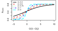
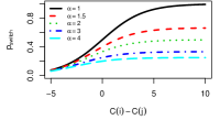
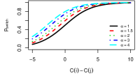
Figure 1. Dependence of the switching probabilities on the parameters and on the cost difference. Left panel: $p_{switch}$ for $\alpha=1.2$. Middle panel: $p_{switch}$ for $\beta=0.5$. Right panel: $p_{switch\,|\,imitate}$ for $\beta=0.5$.

Let us also mention that the same effect of open-mindedness can be achieved by considering large negative values for $\gamma$ in (11). To see this, recall Lemma 2 and note that

$$\begin{split}q_{switch}(i\rightarrow j)&=\mu+\frac{\nu}{\alpha+e^{-\beta(C(i)-C(j))+\gamma}}=\mu+\frac{\nu}{\alpha+e^{\gamma}e^{-\beta(C(i)-C(j))}}\\ &=\mu+\frac{\nu e^{-\gamma}}{\alpha e^{-\gamma}+e^{-\beta(C(i)-C(j))}}.\end{split}$$

In [47], functional forms for the switching probabilities as in (11) for $\mu=0$ and $\nu=\alpha=1$ were considered. The authors suggested that positive values of $\gamma$ represent inertia and negative values of $\gamma$ represent “eagerness to switch.” In the context of (11) the relation between $\gamma$ and inertia is not straightforward as low values of both $\mu$ and $\nu$ also give small overall switching probabilities. However, the above calculations do show a direct correspondence between high values of $\alpha$ and negative values of $\gamma$, with both of them having a plausible interpretation in terms of open-mindedness.

4. Theoretical analysis of the model

4.1. Equilibria in our model

Let $J:[0,1]\rightarrow[0,1]$ denote the updating function that maps $V_{n}$ to $V_{n+1}$. This function $J$ is continuous.

If $V_{n}=1$, then all individuals vaccinate, and if $V_{n}=0$, then nobody vaccinates. In either case, no player can switch strategies, since there is nobody in the population to imitate who would follow another strategy. So $J(0)=0$, $J(1)=1$, and $V^{**}:=0$, $V^{***}:=1$ are always equilibria.

However, we would be more interested in interior equilibria $V^{*}\in(0,1)$ for our model. Note that in our conceptualization of imitation there is always a positive probability that a player will stick with the current strategy rather than imitate another one, even if that other strategy gave a vastly lower cost. Thus $J(V)=0$ only if $V=0$ and $J(V)=1$ only if $V=1$, which means that the interior $(0,1)$ is invariant under $J$. If both $V^{**}$ and $V^{***}$ are repelling, then the updating function $J$ maps some interval $[\varepsilon,1-\varepsilon]$ into itself, and at least one such interior equilibrium $V^{*}$ is guaranteed to exist by Brouwer’s fixed point theorem.

The equilibrium $V^{***}=1$ is always repelling. To see this, consider $V_{n}\in[V_{hit},1)$. For very large population sizes $N$, we will observe approximately $V_{n}(1-V_{n})N$ comparisons that may induce a player to switch from vaccinating to not vaccinating, and the same number of comparisons that may induce a player to switch from not vaccinating to vaccinating. In all these comparisons, players who vaccinated will have born a positive cost, while players who did not vaccinate will not have born any cost. Thus for any choice of the parameters $\alpha,\beta$ we will observe more switches from vaccinating to not vaccinating than vice versa, and it follows that $V_{n+1}<V_{n}$.

Thus if $V^{*}$ exists, it must be in the interval $(0,V_{hit})$. Lemma 5 below shows that an interior equilibrium exists in our model only if $V^{**}=0$ is repelling and gives precise conditions on the parameters for when this is the case. Lemma 4 below shows that if an interior equilibrium $V^{*}$ exists, it must be unique.

The following theorem is the main result of this paper. It shows that for suitable choices of $\alpha$ and $\beta$ the interior equilibrium $V^{*}$ will be arbitrarily close to the societal optimum $V_{hit}$.

Theorem 3.

Fix any $0\leq V^{-}<V_{hit}$ and assume the parameters $\alpha,\beta$ of our model satisfy the inequalities

(15) $$1-e^{-2\beta(c_{i}-c_{v})}-\frac{2(1-x(V^{-}))}{x(V^{-})}e^{-\beta(c_{i}-2c_{v})}>0.$$

(16) $$\alpha>\mbox{max}\{1,\ e^{\beta(c_{i}-c_{v})}+e^{-\beta(c_{i}-c_{v})}-2e^{\beta c_{v}}-2e^{-\beta c_{v}}\}.$$

Then

• If $0<V_{n}<V^{-}$, then $V_{n+1}>V_{n}$.

• If an interior equilibrium $V^{*}$ exists, then $V^{*}\geq V^{-}$.

Proof: Note that it suffices to prove part (a); part (b) is then an immediate consequence.

Let $V^{-},\alpha,\beta$ be as in the assumption, and let $V_{n}<V^{-}$. We will show that the sign of $\Delta(n):=V_{n+1}-V_{n}$ is positive. Let $p_{switch}^{u}$ and $p_{switch}^{v}$ denote the conditional probabilities that a player will switch strategies if that player did not vaccinate or did vaccinate in season $n$, respectively. Then $p_{switch}^{u}=V_{n}p_{switch}(u\rightarrow v)$ and $p_{switch}^{v}=(1-V_{n})p_{switch}(v\rightarrow u)$, so that

$$\begin{split}\Delta(n)&=V_{n+1}-V_{n}\\ &=[1-V_{n}]p_{switch}^{u}-V_{n}p_{switch}^{v}\\ &=\left[(1-V_{n})V_{n}x_{n}\frac{1}{\alpha+e^{-\beta(c_{i}-c_{v})}}+(1-V_{n})V_{n}(1-x_{n})\frac{1}{\alpha+e^{-\beta(0-c_{v})}}\right]\\ &\ \ \ \ -\left[V_{n}(1-V_{n})x_{n}\frac{1}{\alpha+e^{-\beta(c_{v}-c_{i})}}+V_{n}(1-V_{n})(1-x_{n})\frac{1}{\alpha+e^{-\beta(c_{v}-0)}}\right]\\ &=(1-V_{n})V_{n}\left[\frac{x_{n}}{\alpha+e^{-\beta(c_{i}-c_{v})}}+\frac{1-x_{n}}{\alpha+e^{\beta c_{v}}}-\frac{x_{n}}{\alpha+e^{-\beta(c_{v}-c_{i})}}-\frac{1-x_{n}}{\alpha+e^{-\beta c_{v}}}\right]\\ &=(1-V_{n})V_{n}\left[\frac{x_{n}(\alpha+e^{-\beta(c_{v}-c_{i})})-x_{n}(\alpha+e^{-\beta(c_{i}-c_{v})})}{(\alpha+e^{-\beta(c_{i}-c_{v})})(\alpha+e^{-\beta(c_{v}-c_{i})})}\right]\\ &\ \ \ \ +(1-V_{n})V_{n}\left[\frac{(1-x_{n})(\alpha+e^{-\beta c_{v}})-(1-x_{n})(\alpha+e^{\beta c_{v}})}{(\alpha+e^{\beta c_{v}})(\alpha+e^{-\beta c_{v}})}\right]\\ &=(1-V_{n})V_{n}\left[\frac{x_{n}(e^{\beta(c_{i}-c_{v})}-e^{-\beta(c_{i}-c_{v})})}{(\alpha+e^{-\beta(c_{i}-c_{v})})(\alpha+e^{\beta(c_{i}-c_{v})})}+\frac{(1-x_{n})(e^{-\beta c_{v}}-e^{\beta c_{v}})}{(\alpha+e^{\beta c_{v}})(\alpha+e^{-\beta c_{v}})}\right]\\ &=\frac{(1-V_{n})V_{n}}{(\alpha+e^{\beta c_{v}})(\alpha+e^{-\beta c_{v}})}\left[quot(\alpha,\beta)x_{n}(e^{\beta(c_{i}-c_{v})}-e^{-\beta(c_{i}-c_{v})})+(1-x_{n})(e^{-\beta c_{v}}-e^{\beta c_{v}})\right],\end{split}$$

where

$$quot(\alpha,\beta)=\frac{(\alpha+e^{\beta c_{v}})(\alpha+e^{-\beta c_{v}})}{(\alpha+e^{\beta(c_{i}-c_{v})})(\alpha+e^{-\beta(c_{i}-c_{v})})}.$$

Let

$$f(\alpha,\beta)=quot(\alpha,\beta)x_{n}(e^{\beta(c_{i}-c_{v})}-e^{-\beta(c_{i}-c_{v})})+(1-x_{n})(e^{-\beta c_{v}}-e^{\beta c_{v}}).$$

Now to show that $\Delta(n)>0$, it suffices to show that $f(\alpha,\beta)>0$.

For $\beta,V_{n}$ as in the assumptions we have $x_{n}>x(V^{-})$, and hence

$$\begin{split}1-e^{-2\beta(c_{i}-c_{v})}-\frac{2(1-x(V^{-}))}{x(V^{-})}e^{-\beta(c_{i}-2c_{v})}&>0,\\ 1-e^{-2\beta(c_{i}-c_{v})}-\frac{2(1-x_{n})}{x_{n}}e^{-\beta(c_{i}-2c_{v})}&>0,\\ 1-e^{-2\beta(c_{i}-c_{v})}+\frac{2(1-x_{n})}{x_{n}}e^{-\beta c_{i}}-\frac{2(1-x_{n})}{x_{n}}e^{-\beta(c_{i}-2c_{v})}&>0.\end{split}$$

Then

$$\begin{split}&\frac{1}{2}x_{n}(e^{\beta(c_{i}-c_{v})}-e^{-\beta(c_{i}-c_{v})})+(1-x_{n})(e^{-\beta c_{v}}-e^{\beta c_{v}})\\ &=\frac{x_{n}}{2}e^{\beta(c_{i}-c_{v})}\left[1-e^{-2\beta(c_{i}-c_{v})}+\frac{2(1-x_{n})}{x_{n}}e^{-\beta c_{i}}-\frac{2(1-x_{n})}{x_{n}}e^{-\beta(c_{i}-2c_{v})}\right]>0.\end{split}$$

Moreover, the following inequalities are all equivalent:

$$\begin{split}&quot(\alpha,\beta)=\frac{(\alpha+e^{\beta c_{v}})(\alpha+e^{-\beta c_{v}})}{(\alpha+e^{\beta(c_{i}-c_{v})})(\alpha+e^{-\beta(c_{i}-c_{v})})}>\frac{1}{2}\\ &2\alpha^{2}+(2e^{\beta c_{v}}+2e^{-\beta c_{v}})\alpha+2>\alpha^{2}+(e^{\beta(c_{i}-c_{v})}+e^{-\beta(c_{i}-c_{v})})\alpha+1\\ &\alpha^{2}+(2e^{\beta c_{v}}+2e^{-\beta c_{v}}-e^{\beta(c_{i}-c_{v})}-e^{-\beta(c_{i}-c_{v})})\alpha+1>0\end{split}$$

Thus for $\alpha>\mbox{max}\{1,\ e^{\beta(c_{i}-c_{v})}+e^{-\beta(c_{i}-c_{v})}-2e^{\beta c_{v}}-2e^{-\beta c_{v}}\}$ we have

$$quot(\alpha,\beta)>\frac{1}{2}.$$

Then

$$\begin{split}f(\alpha,\beta)&=quot(\alpha,\beta)x_{n}(e^{\beta(c_{i}-c_{v})}-e^{-\beta(c_{i}-c_{v})})+(1-x_{n})(e^{-\beta c_{v}}-e^{\beta c_{v}})\\ &>\frac{1}{2}x_{n}(e^{\beta(c_{i}-c_{v})}-e^{-\beta(c_{i}-c_{v})})+(1-x_{n})(e^{-\beta c_{v}}-e^{\beta c_{v}})\\ &>0.\end{split}$$

$\Box$

Lemma 4.

There can be at most one equilibrium $V^{*}$ in the interval $(0,1)$.

Proof: In this argument we will treat $x$ as a variable that is a function of $V$ rather than of $n$. Recall that this function is strictly decreasing, and hence invertible, on the interval $[0,V_{hit}]$. Consider the functions:

(17) $$\begin{split}g(x)&:=quot(\alpha,\beta)(e^{\beta(c_{i}-c_{v})}-e^{-\beta(c_{i}-c_{v})})x+(1-x)(e^{-\beta c_{v}}-e^{\beta c_{v}}),\\ G(V)&:=quot(\alpha,\beta)(e^{\beta(c_{i}-c_{v})}-e^{-\beta(c_{i}-c_{v})})x(V)+(1-x(V))(e^{-\beta c_{v}}-e^{\beta c_{v}}),\end{split}$$

where $quot(\alpha,\beta)$ is as in the proof of Theorem 3. It follows from our calculations of $\Delta(n)$ in that proof that at an interior equilibrium $V^{*}$ with $x^{*}:=x(V^{*})$ we must have $g(x^{*})=G(V^{*})=0$.

Note that $g(x)$ is a linear function with slope

(18) $$m=quot(\alpha,\beta)(e^{\beta(c_{i}-c_{v})}-e^{-\beta(c_{i}-c_{v})})+e^{\beta c_{v}}-e^{-\beta c_{v}}>0.$$

Thus the system can have at most one interior equilibrium. $\Box$

Lemma 5.

The following conditions are equivalent:

(a) An interior equilibrium $V^{*}\in(0,V_{hit})$ exists.

(b) The equilibrium $V^{**}=0$ is repelling.

(c) One of the following equivalent inequalities holds:

(19) $$\begin{split}&quot(\alpha,\beta)x(0)(e^{\beta(c_{i}-c_{v})}-e^{-\beta(c_{i}-c_{v})})+(1-x(0))(e^{-\beta c_{v}}-e^{\beta c_{v}})>0,\\ &x(0)\left(quot(\alpha,\beta)\left(e^{\beta(c_{i}-c_{v})}-e^{-\beta(c_{i}-c_{v})}\right)+e^{\beta c_{v}}-e^{-\beta c_{v}}\right)>e^{\beta c_{v}}-e^{-\beta c_{v}},\\ x(0)&>\frac{1}{quot(\alpha,\beta)\left(\frac{e^{\beta(c_{i}-c_{v})}-e^{-\beta(c_{i}-c_{v})}}{e^{\beta c_{v}}-e^{-\beta c_{v}}}\right)+1}.\end{split}$$

Proof: Let $g(x),G(V)$ be defined as in (17). Then the conditions in part (c) are simply saying that $g(x(0))=G(0)>0$.

Here $x(0)=x(V^{**})$ is the predicted final size of an outbreak with no vaccination whatsoever. Note that the function $g(x)$ is linear in $x$ and increasing by (18), while $x(V)$ is nonincreasing, and strictly decreasing on $[0,V_{hit}]$. Thus $G(V)$ will be strictly decreasing on the interval $[0,V_{hit}]$. Since $x(V_{hit})=0$ and thus

$$G(V_{hit})=e^{-\beta c_{v}}-e^{\beta c_{v}}<0,$$

it follows from the IVT that $V^{*}$ exists if, and only if, $G(0)>0$.

The updating in our model can be entirely understood in terms of the continuous function $J$ such that $V_{n+1}=J(V_{n})$. Here and in the next subsection we will work with the following formula for this function:

(20) $$\begin{split}H(V)&:=\frac{(1-V)V}{(\alpha+e^{\beta c_{v}})(\alpha+e^{-\beta c_{v}})},\\ J(V)&:=V+H(V)G(V).\end{split}$$

Thus when $G(0)>0$, then $J(\varepsilon)>\varepsilon$ for sufficiently small $\varepsilon>0$ and $V^{**}=0$ will be repelling. On the other hand, when $G(0)\leq 0$, then we must have $G(V)<0$ for all $V\in(0,1]$, the equilibrium $V^{**}$ will be locally asymptotically stable and globally attracting on $[0,1)$, while $V^{*}$ does not exist. $\Box$

Note that criterion (19) is different from the codition $c_{v}\geq c_{i}x(0)$ that makes not vaccinating the rational choice for all players. Similarly to Theorem 3, this implies that in our model we can have an equilibrium vaccination coverage that exceeds the Nash equilibrium. For a numerical example, see Subsubsection 5.1.1.

4.2. Stability of interior equilibria

Now let us assume that the interior equilibrium $V^{*}$ exists and let us investigate its stability, and also whether trajectories that start near enough $V^{*}$ would approach this equilibrium monotonically. We will work with the function $J$ defined in (20).

A sufficient condition for stability of $V^{*}$ is given by

(21) $$-1<\frac{dJ}{dV}(V^{*})<1.$$

Similarly, a sufficient condition for monotone approach to $V^{*}$ is given by

(22) $$0<\frac{dJ}{dV}(V^{*})<1.$$

By differentiating $J$ with respect to $V$ we find that:

(23) $$\begin{split}\frac{dJ}{dV}(V^{*})&=1+\frac{dH}{dV}(V^{*})G(V^{*})+H(V^{*})\frac{dG}{dV}(V^{*})\\ &=1+\frac{dH}{dV}(V^{*})(0)+H(V^{*})\frac{dG}{dV}(V^{*})=1+H(V^{*})\frac{dG}{dV}(V^{*}),\\ &=1+H(V^{*})m\frac{dx}{dV}(V^{*})\\ &<1.\end{split}$$

Since $H(V^{*})>0$ for $V^{*}\in(0,1)$, the last inequality in (23) follows from (18) and the fact that $x(V)$ is a strictly decreasing function on $[0,V_{hit}]$; no special assumptions on $\alpha,\beta$ needed so far.

Now consider the term $H(V^{*})m\frac{dx}{dV}(V^{*})$ of the third line of (23). This term is always negative. For local stability of $V^{*}$ we need

(24) $$-2\leq H(V^{*})m\frac{dx}{dV}(V^{*}),$$

and for monotone approach we need that

(25) $$-1\leq H(V^{*})m\frac{dx}{dV}(V^{*}).$$

It remains to investigate bounds on $\frac{dx}{dV}(V)$. We can argue here as follows: In the absence of vaccination, $x(R_{0})$ is a function of $R_{0}$ that for $R_{0}>1$ takes the value $x$ that is the unique solution of the first line of (10) in the interval $(0,1)$. (Here and in the remainder of this subsection we use $R$ to indicate a variable and $R_{0}$ for the fixed parameter of our model.) When we administer perfectly effective vaccine to a fraction $V$ of the population, we decrease in effect the expected number of secondary infections caused by an index case in the susceptible population by a factor of $1-V$, so that the dynamics boil down to an SIR-model with

(26) $$R_{0}^{V}=R_{0}(1-V),\qquad\mbox{or, equivalently,}\qquad\frac{R_{0}}{R_{0}^{V}}=\frac{1}{1-V}.$$

Note that, in particular, by solving this equation for $R_{0}^{V_{hit}}=1$, we obtain the herd immunity threshold $V_{hit}=1-\frac{1}{R_{0}}$. From the chain rule we get

(27) $$\frac{dx}{dV}(V^{*})=\frac{dx}{dR}(x(R_{0}^{V^{*}}))\frac{dR_{0}^{V}}{dV}(V^{*})=-R_{0}\frac{dx}{dR}(x(R_{0}^{V^{*}})).$$

We will now use $x$ as the variable for the final size of the outbreak in the SIR model with parameter $R=R_{0}^{V}$. By implicitly differentiating the function $x(R)$ that is defined by the first line of (10) we get

(28) $$\begin{split}-\frac{dx}{dR}&=(-R_{0}\frac{dx}{dR}-x)e^{-Rx}=\left(-R\frac{dx}{dR}-x\right)(1-x),\\ (R(1-x)-1)\frac{dx}{dR}&=x^{2}-x,\\ \frac{dx}{dR}&=\frac{x^{2}-x}{R(1-x)-1}=\frac{x}{\frac{1}{1-x}-R}.\end{split}$$

We need to keep in mind that in (28) the variable $x$ is a function of $R$. So our problem will involve working with bounds for the expression

(29) $$\begin{split}-R\frac{dx}{dR}&=\frac{R(x-x^{2})}{R(1-x)-1}=\frac{Rx(1-x)}{R(1-x)-1}=\frac{x}{1-\frac{1}{R(1-x)}}.\end{split}$$

that we get from combining (27) with (28).

Proposition 6.

For all $x\in(0,1)$ the following inequalities hold:

$$-2<\frac{x}{1-\frac{1}{R(1-x)}}<0$$

Proof: By the first line of (10), we have

$$R=-\frac{\ln(1-x)}{x}.$$

Then the inequalities we want to prove can be written as

$$-2<\frac{x}{1+\frac{x}{(1-x)\ln(1-x)}}=\frac{(x-x^{2})\ln(1-x)}{(1-x)\ln(1-x)+x}<0,$$

and the result follows from Proposition 8 of the first part of the Appendix 7. $\Box$

This gives us estimates of (29), but what we really need are bounds on $H(V^{*})m\frac{dx}{dV}(V^{*})$. Let

$$S(\alpha,\beta):=\frac{e^{\beta(c_{i}-c_{v})}-e^{-\beta(c_{i}-c_{v})}}{(\alpha+e^{\beta(c_{i}-c_{v})})(\alpha+e^{-\beta(c_{i}-c_{v})})}+\frac{e^{\beta c_{v}}-e^{-\beta c_{v}}}{(\alpha+e^{\beta c_{v}})(\alpha+e^{-\beta c_{v}})}.$$

By the definition of $quot(\alpha,\beta)$ we get from (18) and (20) that

(30) $$\begin{split}H(V^{*})m&=(1-V^{*})V^{*}\left(\frac{e^{\beta(c_{i}-c_{v})}-e^{-\beta(c_{i}-c_{v})}}{(\alpha+e^{\beta(c_{i}-c_{v})})(\alpha+e^{-\beta(c_{i}-c_{v})})}+\frac{e^{\beta c_{v}}-e^{-\beta c_{v}}}{(\alpha+e^{\beta c_{v}})(\alpha+e^{-\beta c_{v}})}\right),\\ H(V^{*})m&=(1-V^{*})V^{*}S(\alpha,\beta).\end{split}$$

Note that the following inequalities always hold for $0<V^{*}<1$:

(31) $$0<S(\alpha,\beta)<\frac{2}{\alpha}\qquad\mbox{and}\qquad 0<H(V^{*})m<\frac{2}{\alpha}(1-V^{*})V^{*}.$$

Then

(32) $$\begin{split}H(V^{*})m\frac{dx}{dV}(V^{*})&=H(V^{*})m\left(-R_{0}\frac{dx}{dR}\left(x\left(R_{0}^{V^{*}}\right)\right)\right)\\ &=H(V^{*})m\frac{R_{0}}{R_{0}^{V^{*}}}\left(-R_{0}^{V^{*}}\frac{dx}{dR}\left(x\left(R_{0}^{V^{*}}\right)\right)\right)\\ &=(1-V^{*})V^{*}S(\alpha,\beta)\frac{R_{0}}{R_{0}^{V^{*}}}\left(-R_{0}^{V^{*}}\frac{dx}{dR}\left(x\left(R_{0}^{V^{*}}\right)\right)\right)\\ &=(1-V^{*})V^{*}S(\alpha,\beta)\frac{R_{0}}{R_{0}^{V^{*}}}\frac{x(R_{0}^{V^{*}})}{1-\frac{1}{R_{0}^{V^{*}}(1-x(R_{0}^{V^{*}}))}}\\ &=V^{*}S(\alpha,\beta)\frac{x(R_{0}^{V^{*}})}{1-\frac{1}{R_{0}^{V^{*}}(1-x(R_{0}^{V^{*}}))}},\end{split}$$

where the last line follows from (26).

If $V^{*}<S(\alpha,\beta)^{-1}$ and $0<x(R_{0}^{V^{*}})<1$, then by (32) and Proposition 6 we will have

$$H(V^{*})m\frac{dx}{dV}(V^{*})=V^{*}S(\alpha,\beta)\frac{x(R_{0}^{V^{*}})}{1-\frac{1}{R_{0}^{V^{*}}(1-x(R_{0}^{V^{*}}))}}>-2\\$$

Similarly, if $V^{*}<\frac{1}{2}S(\alpha,\beta)^{-1}$ and $0<x(R_{0}^{V^{*}})<1$, we will have

$$H(V^{*})m\frac{dx}{dV}(V^{*})=V^{*}S(\alpha,\beta)\frac{x(R_{0}^{V^{*}})}{1-\frac{1}{R_{0}^{V^{*}}(1-x(R_{0}^{V^{*}}))}}>-1.$$

By (31) we have $S(\alpha,\beta)<\frac{2}{\alpha}$. Thus whenever $\alpha\geq 2$ we will have $V^{*}<1<S(\alpha,\beta)^{-1}$. Similarly, as long as $\alpha\geq 4$, we have $V^{*}<1<0.5S(\alpha,\beta)^{-1}$. This proves the following result:

Lemma 7.

Consider the restricted model with imitations and parameters such that the interior equilibrium $V^{*}\in(0,1)$ exists. Then

• $\alpha\geq 2$ is a sufficient condition for local stability of $V^{*}$.

• $\alpha\geq 4$ is a sufficient condition for monotone approach to $V^{*}$.

Remark 1.

(a) The conditions in Lemma 7 are sufficient, but not necessary. However, as our results reported in 5.1 show, some conditions on the parameters are needed even for stability. Thus we will leave it as an open problem to find more precise conditions for local stability of $V^{*}$ and monotone approach to this equilibrium.

(b) It is of interest to observe here that when we extend our model to allow for switching probabilities of the form (2), then the expression for the updating function $J$ changes. As long as $\gamma=0$ it will take the form

(33) $$J(V)=V+\nu H(V)G(V),$$

where the symbols $H$ and $G$ denote the same funtions as in (20). This follows from the proof of Lemma 2. While the parameter $\nu$ will not affect existence and location of the interior equilibrium $V^{*}$, it will modify the calculation of the derivative of $J$ so that in analogy to (23) we obtain

(34) $$\frac{dJ}{dV}(V^{*})=1+\nu H(V^{*})m\frac{dx}{dV}(V^{*}).$$

It follows that in versions of our model that allow larger values of $\nu$, such as a version that would use (14) instead of (3), we might see instability of $V^{*}$ and sustained oscillations even when $\alpha$ is large.

5. Numerical results

All numerical results included in this section were obtained by setting the cost parameters to $c_{v}=1$ and $c_{i}=12$. Some details about the software that we used in these explorations can be found in Appendix B 8.

5.1. Stability of equilibria

5.1.1. Stability of $V^{**}=0$

Lemma 5 predicts that a population that starts with $V(0)\in(0,1)$ will evolve towards the equilibrium $V^{**}=0$ where nobody vaccinates if, and only if

(35) $$x(0)\leq\frac{1}{quot(\alpha,\beta)\left(\frac{e^{\beta(c_{i}-c_{v})}-e^{-\beta(c_{i}-c_{v})}}{e^{\beta c_{v}}-e^{-\beta c_{v}}}\right)+1}.$$

Interestingly enough, this condition is different from the inequality

(36) $$x(0)\leq\frac{c_{v}}{c_{i}}$$

that gives the condition under which not vaccinating is the rational choice for the entire population.

Suppose $c_{i}=12$ and $c_{v}=1$. Then (36) becomes

(37) $$x(0)\leq\frac{1}{12}\approx 0.0833.$$

Figure 2 shows a heat map for the dependence of the right-hand side of (35) on $\alpha$ and $\beta$ when $c_{i}=12$ and $c_{v}=1$. When equality holds in (37) so that $V_{Nash}=0$, then in the region below the black curve the equilibrium $V^{**}=0$ becomes repelling, with $V^{*}\in(0,1)$ predicted to exist.

Figure 2. Dependence of the right-hand side of (35) on $\alpha$ and $\beta$ when $c_{i}=12$ and $c_{v}=1$. Created with script lowerbd.m.

5.1.2. Counterexamples to stability of $V^{*}$

In order to identify regions of the parameter space where $V^{*}$ is locally asymptotically stable and where approach to this equilibrium will be monotone, we numerically explored the value of

$$H(V^{*})m\frac{dx}{dV}(V^{*})=V^{*}S(\alpha,\beta)\frac{x(R_{0}^{V^{*}})}{1-\frac{1}{R_{0}^{V^{*}}(1-x(R_{0}^{V^{*}}))}}$$

with our MatLab scripts critical_R0.m and stability_and_approach.m.

For a range of $\beta$ values, we calculated the critical value of $R_{0}$ at which $H(V^{*})m\frac{dx}{dV}(V^{*})=-1$. For $\alpha=3$, such $R_{0}$ was not found for $1\leq\beta\leq 50$. Figures 3 and 4 display the results for $\alpha=1$ and $\alpha=2$.

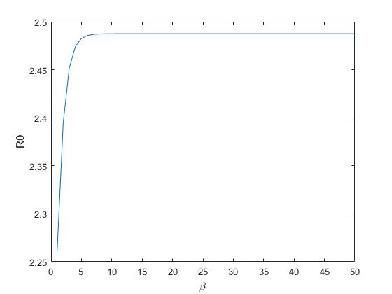
Figure 3. Critical value of $R_{0}$ at which $H(V^{*})m\frac{dx}{dV}(V^{*})=-1$ for $\alpha=1$.

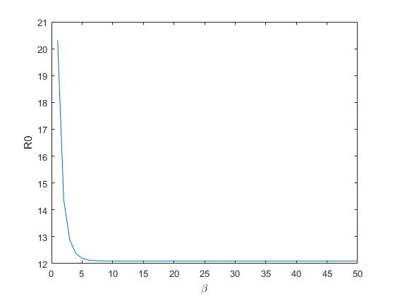
Figure 4. Critical value of $R_{0}$ at which $H(V^{*})m\frac{dx}{dV}(V^{*})=-1$ for $\alpha=2$.

In order to see how the seemingly strange inversion of shapes in Figures 3 and 4 occurs, let us consider Figure 5 that shows what happens if we gradually increase $\alpha$.

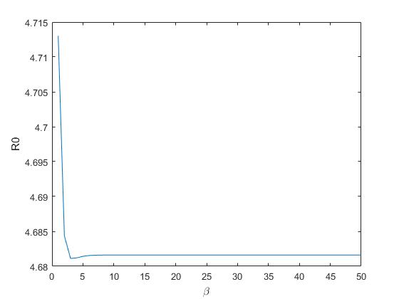
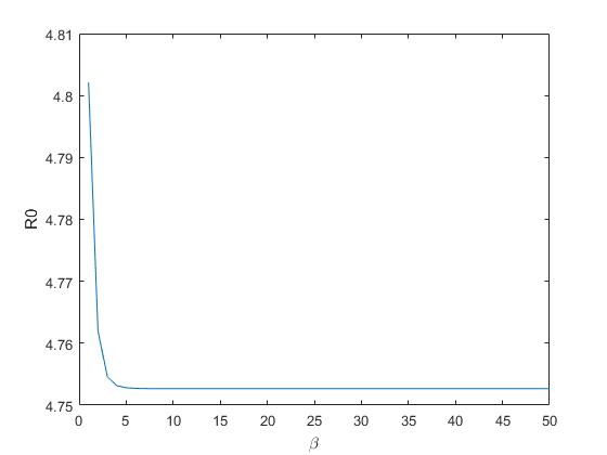
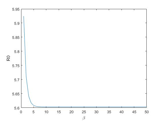
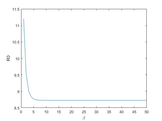
Figure 5. Critical value of $R_{0}$ at which $H(V^{*})m\frac{dx}{dV}(V^{*})=-1$ for
$\alpha=1,1.1,1.2,1.3,1.4,1.5,1.55,1.56,1.565,1.57,1.575,1.58,1.59,1.6,1.7,1.8,1.9,2$

Similarly, for $\alpha=1$ and for a range of $\beta$ values, we calculated the critical value of $R_{0}$ at which $H(V^{*})m\frac{dx}{dV}(V^{*})=-2$. Figure 6 displays the results:

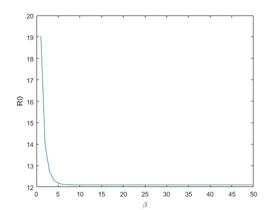
Figure 6. Critical value of $R_{0}$ at which $H(V^{*})m\frac{dx}{dV}(V^{*})=-2$ for $\alpha=1$.

These results suggest regions of the parameter space where we would have interior equilibria $V^{*}$ that are not approached monotonically and/or where $V^{*}$ might be unstable. In order to better visualize these regions, we color-coded them by distinguishing values in certain relevant intervals. More specifically, we defined a function $Int\left(H(V^{*})m\frac{dx}{dV}(V^{*})\right)$ in the following way:

• $Int\left(H(V^{*})m\frac{dx}{dV}(V^{*})\right)=-4$ if $H(V^{*})m\frac{dx}{dV}(V^{*})<-2$,

• $Int\left(H(V^{*})m\frac{dx}{dV}(V^{*})\right)=-1.5$ if $-2\leq H(V^{*})m\frac{dx}{dV}(V^{*})<-1.05$,

• $Int\left(H(V^{*})m\frac{dx}{dV}(V^{*})\right)=-0.7$ if $-1.05\leq H(V^{*})m\frac{dx}{dV}(V^{*})<-1$,

• $Int\left(H(V^{*})m\frac{dx}{dV}(V^{*})\right)=-0.5$ if $-1\leq H(V^{*})m\frac{dx}{dV}(V^{*})<0$,

• $Int\left(H(V^{*})m\frac{dx}{dV}(V^{*})\right)=2$ if MatLab cannot find $V^{*}$ in $[0,1]$ for given $\alpha$ and $\beta$, or a $V^{*}$ in $[0,1]$ is found but the corresponding $x(V^{*})$ is not in $(0,1)$,

In Figures 7–9, we plot the resulting color-coded partitions of the parameter space, together with some sample trajectories of $V_{n}$ in regions of interest that were calculated using our code FluVacc.

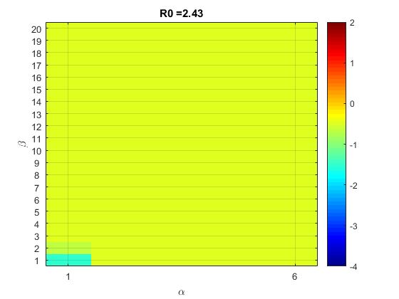
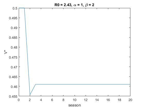
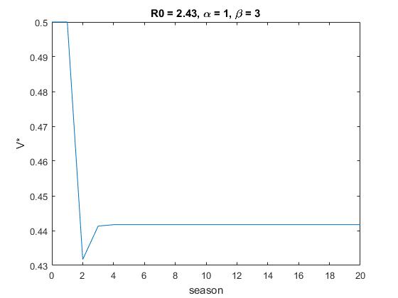
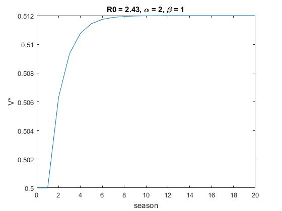
Figure 7. Color map of $Int\left(H(V^{*})m\frac{dx}{dV}(V^{*})\right)$ and sample trajectories for $\mathcal{R}_{0}=2.43$.

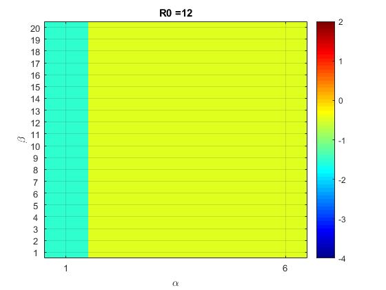
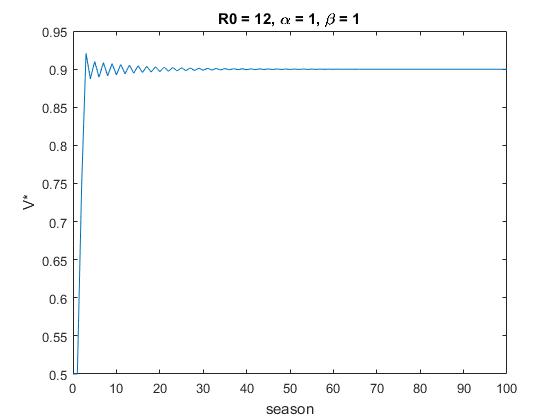
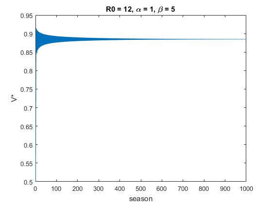
Figure 8. Color map of $Int\left(H(V^{*})m\frac{dx}{dV}(V^{*})\right)$ and sample trajectories for $\mathcal{R}_{0}=12$.

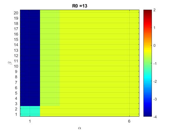
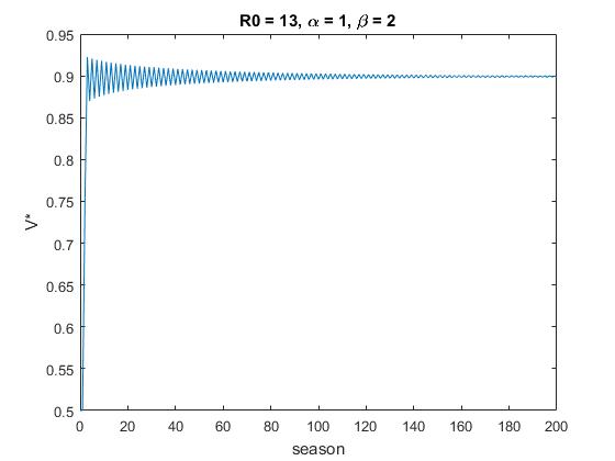
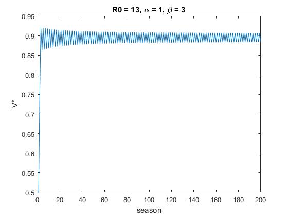
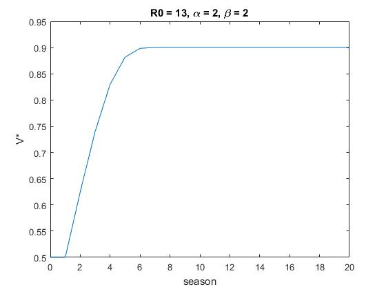
Figure 9. Color map of $Int\left(H(V^{*})m\frac{dx}{dV}(V^{*})\right)$ and sample trajectories for $\mathcal{R}_{0}=13$.

5.2. Predicted interior equilibria $V^{*}$

The figures in this subsection show the interior equilibria $V^{*}\in(0,1)$ of the vaccination coverage that we get as outputs of our script V_G0_2v_fsolve.m that is briefly described in Subsection 8.2.2 of Appendix B. Figure 10 shows the dependence of $V^{*}$ on $\alpha$ and $\beta$ in the form of heat maps for selected values of $\mathcal{R}_{0}$.

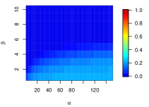
(a) $R_{0}=1.3$

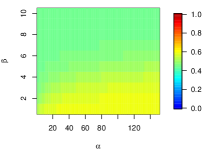
(b) $R_{0}=2.5$

(c) $R_{0}=5.0$

Figure 10. Dependence of $V^{*}$ on $\alpha$ and $\beta$ via theoretical results described in Section 8.2.2 for $c_{v}=1$ and $c_{i}=12$.

5.3. Simulation results

Figure 11 presents the results of direct simulation of our difference equation model described in Section 2 using the script simulation_script.m that is briefly described in Subsection 8.3.2 of Appendix B. For each combination of parameters $\alpha$ and $\beta$ the model is simulated to equilibrium (using a stopping criteria of $|V_{n+1}-V_{n}|<10^{-5}$) with the resulting vaccination coverage, $V^{*}$, recorded. Even though this stopping criterion might introduce some small errors, vaccination coverages from direct numerical simulation (Figure 11) match those predicted by the theoretical analysis (Figure 10) remarkably closely. The contour on each surface depicts where the model with imitation matches the vaccine coverage at the Nash equilibrium, which is labeled on the contour. Therefore, we see that vaccination coverage exceeds that of the Nash equilibrium for combinations of $\alpha$ and $\beta$ that lie below and to the right of this threshold.

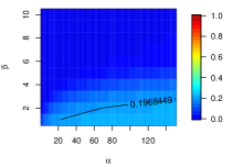
(a) $R_{0}=1.3$

(b) $R_{0}=2.5$

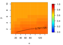
(c) $R_{0}=5.0$

Figure 11. Dependence of $V^{*}$ on $\alpha$ and $\beta$ via numerical simulation of approach to interior equilibrium. $c_{v}=1$, $c_{i}=12$, $V_{0}=0.5$ and $tol=10^{-5}$.

6. Discussion

The problem of designing effective public policy for inducing people to vaccinate against vaccine-preventable diseases is of great societal urgency [29]. To solve this problem, we need to understand how people really make vaccination decisions and how certain factors that enter this process influence the outcome.

The work presented here focuses on the role of imitation of successful others, which has been well-documented to be an important component of human decision-making [2]. Our model builds on the version of the model in [16] that assumed uniform mixing in the population. The only difference is including an additional parameter $\alpha$ in the functional form for the probability of switching to another strategy. This parameter can be loosely interpreted as a degree of open-mindedness and has parallels in functional forms of these probabilities that were empirically derived in [37].

Our results demonstrate that for sufficiently high values of $\alpha$ the predicted equilibrium coverage will be arbitrarily close to the societally optimal value $V_{hit}$ that gives herd immunity. They were confirmed both analytically for large regions of the parameter space in Theorem 3 and by numerical explorations of the equilibria predicted in the proof of this theorem (Subsection 5.2) and the equilibria that are being approached in simulated evolution of the vaccination coverages (Subsection 5.3). They stand in stark contrast to the results reported in [16] for the standard Fermi functions, which under the uniform mixing assumption imitation leads to vaccination coverage even below the Nash equilibrium when the cost of vaccination is small relative to the cost of infection. As we deliberately kept our model as basic as possible and excluded all other factors, such as community structure, incentives, or misperceptions, these radical differences in the predictions can be due only to choosing a high value of $\alpha$. We conclude that “open-minded imitation,” based on switching probabilities of the form (3) with suitable choices of $\alpha$, provides a possible avenue for attenuating the vaccination dilemma.

The findings presented here open up a number of avenues for future research, in at least four directions. The first would be to try tightening some of our theoretical results by proving analogues under weaker assumptions. More specifically, conditions (15) and (16) of Theorem 3 are sufficient, but not necessary, as our numerical explorations in Subsections 5.2 and 5.3 indicate that the conclusion of the theorem remains valid under significantly weaker assumptions. Similarly, Lemma 7 gives only sufficient conditions for stability of the interior equilibrium $V^{*}$ and monotone approach to it. Our numerical explorations in Subsection 5.1 indicate that these conditions already give us a qualitatively accurate picture; it would be of some intrinsic mathematical interest to find conditions that are simultaneously sufficient and necessary.

The second direction would be to examine the effect of the parameter $\alpha$ in extensions of our model that incorporate a number of additional aspects of voluntary vaccination dynamics that have been deliberately set aside here. We have already done some preliminary work on extending our model to the case when the vaccine has an efficacy of less than 100% and found a similar pattern as the one reported here in that equilibrium coverage can get arbitrarily close to the societal optimum. However, the dependence of the optimal choice of $\alpha$ on $\beta$ is more complicated than in Theorem 3 and still needs to be worked out in more detail. Other aspects that might be incorporated into more detailed versions of our model are restrictions of disease transmission and/or imitation to edges of contact networks, as has already been studied for the case of classical Fermi functions in [16] and a number of related papers; see [39] for a review. Similarly, one can study the effects of a mixture of rational decision-making and imitation [12, 31], incentives [27, 44, 45], misperceptions of costs [4, 9, 10, 32, 38], altruism [34, 36, 46], peer pressure [23, 42], presence of individuals who remain committed to vaccinating or not vaccinating without ever imitating others [19, 28], the effects of other available control measures or treatment options [1, 8, 24, 26, 27, 41], or variability of $\mathcal{R}_{0}$ from season to season. One can also study the effects of our parameter $\alpha$ when imitation is based on comparison with the average cost of a larger sample of other individuals [18, 23, 25, 27], or when weighted averages of costs over a number of previous seasons are being compared [43].

The third direction would be to study applications of our functional form (3) to domains other than vaccination games. The paper [47] considers prisoner’s dilemma games in a finite population with switching probabilities of the form $\frac{1}{1+e^{-\beta(C(i)-C(j))-\tau_{s}}}$, where $\tau_{s}$ depends on the strategy of the focal player. These can be considered rescaled versions of (3) (see the discussion at the end of Subsection 3.2). The authors of [47] obtained a number of analytical results, but their focus is on fixation probabilities, time to fixation, and stochastic stability of the equilibria, which is different from ours. The literature on applications of evolutionary games with the structure of a prisoner’s dilemma is vast, and vaccination games are only a small part of it. So it seems likely that our version of (3) or its counterpart in [47] could find many applications outside of vaccination games. Let us also remark that there may be some applications to evolutionary computation [13] as well. In this field the balance between exploration and exploitation is of paramount importance, and our interpretation of high $\alpha$ as open-mindedness bears some resemblance to shifting this balance towards the former for high values of this parameter.

Finally, it would be important to get a better understanding of how our parameter $\alpha$ relates to actual decision-making by real people and how public policy could enhance more “open-minded” decision-making about vaccination in the sense captured by this parameter. This fourth direction of suggested follow-up work would require a multidisciplinary effort that goes far beyond the realm of mathematical modeling.

7. Appendix A: Some technical results and proof of Theorem 1

7.1. Some technical results

Here we prove some elementary technical facts that are used in several of our arguments.

Proposition 8.

For all $x\in(0,1)$ the following inequalities hold:

(38) $$-2<\frac{(x-x^{2})\ln(1-x)}{x+(1-x)\ln(1-x)}<0.$$

Proof: Let $f(x)=(1-x)\ln(1-x)+x$ be the denominator of the above fraction. Then on $(0,1)$,

$$\begin{split}f^{\prime}(x)&=-\ln(1-x)-(1-x)\frac{1}{1-x}+1=-\ln(1-x)>0,\\ f(x)&>f(0)=0,\\ (x-x^{2})\ln(1-x)&=x(1-x)\ln(1-x)<0.\end{split}$$

Thus, we have proved the inequality on the right-hand side of (38).

For the inequality on the left-hand side of (38), for $x\in(0,1)$,

$$\begin{split}&\frac{(x-x^{2})\ln(1-x)}{(1-x)\ln(1-x)+x}>-2\\ &\Leftrightarrow\frac{(x-x^{2})\ln(1-x)+(2-2x)\ln(1-x)+2x}{f(x)}>0\\ &\Leftrightarrow(-x^{2}-x+2)\ln(1-x)+2x>0\\ &\Leftrightarrow\ln(1-x)>\frac{2x}{x^{2}+x-2}.\end{split}$$

Let $h(x)=g_{1}(x)-g_{2}(x)$, where $g_{1}(x)=\ln(1-x)$ and $g_{2}(x)=\frac{2x}{x^{2}+x-2}$. Our goal is to show that $h(x)>0$ on $(0,1)$.

Note that $g_{1}(0)=g_{2}(0)=h(0)=0$. On $(0,1)$,

$$\begin{split}g_{1}^{\prime}(x)&=\frac{1}{x-1}=\frac{(x+2)(x^{2}+x-2)}{(x^{2}+x-2)^{2}}=\frac{x^{3}+3x^{2}-4}{(x^{2}+x-2)^{2}},\\ g_{2}^{\prime}(x)&=\frac{-2x^{2}-4}{(x^{2}+x-2)^{2}},\\ h^{\prime}(x)&=g_{1}^{\prime}(x)-g_{2}^{\prime}(x)=\frac{x^{2}(x+5)}{(x^{2}+x-2)^{2}}>0.\end{split}$$

We conclude that the left hand side of (38) holds. $\Box$

Proposition 9.

The function $f(x):=x+\frac{(x^{2}-x)\ln(1-x)}{x+(1-x)\ln(1-x)}$ is decreasing on $(0,1)$.

Proof: Notice that $f$ can be rewritten as

$$\begin{split}f(x)&=x+\frac{(x^{2}-x)\ln(1-x)}{x+(1-x)\ln(1-x)}\\ &=\frac{x^{2}-(x^{2}-x)\ln(1-x)+(x^{2}-x)\ln(1-x)}{x-(x-1)\ln(1-x)}\\ &=\frac{x^{2}}{x-(x-1)\ln(1-x)}.\end{split}$$

To show that $f(x)$ is decreasing on $(0,1)$, we examine its derivative:

$$\begin{split}f^{\prime}(x)&=\frac{2x(x-(x-1)\ln(1-x))-x^{2}(x-(x-1)\ln(1-x))^{\prime}}{(x-(x-1)\ln(1-x))^{2}}\\ &=\frac{2x^{2}-(2x^{2}-2x)\ln(1-x)-x^{2}(1-1-\ln(1-x))}{(x-(x-1)\ln(1-x))^{2}}\\ &=\frac{2x^{2}-(x^{2}-2x)\ln(1-x)}{(x-(x-1)\ln(1-x))^{2}}.\end{split}$$

The denominator $(x-(x-1)\ln(1-x))^{2}$ of $f^{\prime}(x)$ is always positive on $(0,1)$. Thus it suffices to show that the numerator

$$g(x):=2x^{2}-(x^{2}-2x)\ln(1-x)$$

is negative on $(0,1)$. Observe that

$$\begin{split}g^{\prime}(x)&=4x-\frac{x^{2}-2x}{x-1}-2(x-1)\ln(1-x),\\ &=\frac{3x^{2}-2x}{x-1}-2(x-1)\ln(1-x),\\ g^{\prime\prime}(x)&=\frac{(6x-2)(x-1)-3x^{2}+2x}{(x-1)^{2}}-2-2\ln(1-x),\\ &=\frac{6x^{2}-8x+2-3x^{2}+2x-2x^{2}+4x-2}{(x-1)^{2}}-2\ln(1-x),\\ &=\frac{x^{2}-2x}{(x-1)^{2}}-2\ln(1-x)=1-\frac{1}{(x-1)^{2}}-2\ln(1-x),\\ g^{\prime\prime\prime}(x)&=\frac{2}{(x-1)^{3}}-\frac{2}{x-1}=\frac{2-2x^{2}+4x-2}{(x-1)^{3}}\\ &=\frac{2x(2-x)}{(x-1)^{3}}<0\ \ \mbox{on}\ (0,1).\end{split}$$

Since $g(0)=g^{\prime}(0)=g^{\prime\prime}(0)=0$, we conclude that $g$ is concave down with $g^{\prime}(x)<0$ and $g(x)<0$ on $(0,1)$. $\Box$

7.2. Proof of Theorem 1

We will consider the sign of the derivative

(39) $$\frac{d\,PC}{d\,V}=c_{v}-c_{i}x+\frac{d\,x}{d\,V}c_{i}(1-V).$$

We already know that under the assumptions of the theorem we must have $V_{Nash}\in(0,V_{hit})$. Then $c_{v}-c_{i}x=c_{v}-c_{i}x(V_{Nash})=0$ by the definition of a Nash equilibrium, and $\frac{d\,x}{d\,V}(V_{Nash})<0$. Thus $\frac{d\,PC}{d\,V}(V_{Nash})<0$, which means that the societal cost can be decreased by increasing the vaccination coverage above Nash equilibrium.

For $V\in(0,V_{Nash})$,

$$\begin{split}\frac{dPC}{dV}&=c_{v}-c_{i}x(V)+\frac{dx}{dV}c_{i}(1-V)\\ &\leq c_{v}-c_{i}x(V_{Nash})+\frac{dx}{dV}c_{i}(1-V)=\frac{dx}{dV}c_{i}(1-V)<0.\end{split}$$

This proves part (a).

For the proof of parts (c) and (d), recall that we already know that $V_{opt}\in[0,V_{hit}]$. We only need to exclude the possibility that $V_{opt}=V_{hit}$. It is not immediately clear though whether $\frac{d\,x}{d\,V}(V_{hit})$ exists. Thus we want to investigate

(40) $$\lim_{V\rightarrow V_{hit}^{-}}\frac{d\,PC}{d\,V}(V)=c_{v}+c_{i}(1-V)\lim_{V\rightarrow V_{hit}^{-}}\frac{d\,x}{d\,V}(V).$$

By implicitly differentiating the second line of (10) we obtain:

(41) $$\begin{split}\frac{d\,(1-x)}{d\,V}&=\frac{d}{d\,V}e^{-\mathcal{R}_{0}(1-V)x}\\ -\frac{d\,x}{d\,V}&=e^{-\mathcal{R}_{0}(1-V)x}\frac{d}{d\,V}(-\mathcal{R}_{0}(1-V)x)\\ \frac{d\,x}{d\,V}&=\mathcal{R}_{0}(1-x)\frac{d}{d\,V}\left(x(1-V)\right)\\ \frac{d\,x}{d\,V}&=\mathcal{R}_{0}(1-x)\left((1-V)\frac{d\,x}{d\,V}-x\right)\\ \frac{d\,x}{d\,V}\left(1-\mathcal{R}_{0}(1-x)(1-V)\right)&=-\mathcal{R}_{0}(1-x)x\\ \frac{d\,x}{d\,V}&=\frac{-\mathcal{R}_{0}(1-x)x}{\left(1-\mathcal{R}_{0}(1-x)(1-V)\right)}\\ \frac{d\,x}{d\,V}&=\frac{-\mathcal{R}_{0}(1-x)x}{\left(1+\frac{(1-x)\ln(1-x)}{x}\right)}\\ \frac{d\,x}{d\,V}&=\frac{-\mathcal{R}_{0}(x^{2}-x^{3})}{x+(1-x)\ln(1-x))}\\ \lim_{V\rightarrow V_{hit}^{-}}\frac{d\,x}{d\,V}=\lim_{x\rightarrow 0^{+}}\frac{d\,x}{d\,V}&=\lim_{x\rightarrow 0^{+}}\frac{\mathcal{R}_{0}(x^{3}-x^{2})}{x+(1-x)\ln(1-x)}\\ &\stackrel{{\scriptstyle(H)}}{{=}}\lim_{x\rightarrow 0^{+}}\frac{\mathcal{R}_{0}(3x^{2}-2x)}{1-\ln(1-x)-\frac{1-x}{1-x}}\\ &=\lim_{x\rightarrow 0^{+}}\frac{\mathcal{R}_{0}(3x-2)x}{-\ln(1-x)}=-2\mathcal{R}_{0}.\end{split}$$

Now parts (c) and (d) follow from substituting $-2R_{0}$ for $\lim_{V\rightarrow V_{hit}^{-}}\frac{d\,x}{d\,V}$ and $1-V=1-V_{hit}=\frac{1}{\mathcal{R}_{0}}$ in (40).

For the proof of part (b), notice that in view of the above calculations and of the second line of (10):

(42) $$\begin{split}\frac{d\,PC}{d\,V}&=c_{v}-c_{i}\left(x-(1-V)\frac{d\,x}{d\,V}\right)\\ &=c_{v}-c_{i}\left(x-(1-V)\frac{\mathcal{R}_{0}(x^{3}-x^{2})}{x+(1-x)\ln(1-x)}\right)\\ &=c_{v}-c_{i}\left(x+\frac{(x^{2}-x)\ln(1-x)}{x+(1-x)\ln(1-x)}\right).\end{split}$$

By Proposition 9, the function $f(x):=x+\frac{(x^{2}-x)\ln(1-x)}{x+(1-x)\ln(1-x)}$ is decreasing on $(0,1)$. Moreover, by Proposition 8,

$$0<\frac{(x^{2}-x)\ln(1-x)}{x+(1-x)\ln(1-x)}$$

on $(0,1)$. Thus

$$1<x+\frac{(x^{2}-x)\ln(1-x)}{x+(1-x)\ln(1-x)},$$

and it follows that

$$\frac{d\,PC}{d\,V}=c_{v}-c_{i}\left(x+\frac{(x^{2}-x)\ln(1-x)}{x+(1-x)\ln(1-x)}\right)<c_{v}-c_{i}\leq 0$$

for $0\leq V<V_{hit}$ when $c_{i}\geq c_{v}$. $\Box$

8. Appendix B: Description of our software

We coded several programs that allowed us to numerically explore various aspects of some of our models. Here we give brief descriptions of how they work. The codes themselves and complete documentations are available from the authors upon request.

8.1. Code for predicting stability of interior equilibria

Here we have two scripts.

Our codes for predicting stability of $V^{*}$ is based on estimating the derivative $\frac{d\,J(V)}{d\,V}$ as caclculated in (20) and observing that for local stability of $V^{*}$ we need

(43) $$-2\leq H(V^{*})m\frac{dx}{dV}(V^{*}),$$

while for monotone approach to $V^{*}$ we need

(44) $$-1\leq H(V^{*})m\frac{dx}{dV}(V^{*}).$$

8.1.1. critical_R0.m

For given $\alpha$ and a range of $\beta$ values, this script calculates the critical value of $R_{0}$ at which

$$H(V^{*})m\frac{dx}{dV}(V^{*})=-1\ \mbox{or}\ -2$$

so that damped oscillations near the interior equilibrium $V^{*}$ are predicted to appear/disappear or the local stability of $V^{*}$ is predicted to change. The code plots a graph of the dependence of these critical values on $\beta$. .

8.1.2. stability_and_approach.m

This script explores stability of equilibria for a user-defined range of parameter values $(\alpha,\beta)$ when the other parameters are kept fixed.

For given parameters, the script computes the values of $H(V^{*})m\frac{dx}{dV}(V^{*})$ and compares them with $-1$ to check for predicted oscillations near $V^{*}$ (see (44)) and with $-2$ to check for local asymptotic stability of $V^{*}$ (see (43)).

It outputs a color map of $H(V^{*})m\frac{dx}{dV}(V^{*})$ by distinguishing values in certain relevant intervals. More specifically, it displays colors for the function $Int\left(H(V^{*})m\frac{dx}{dV}(V^{*})\right)$ that we defined in the following way:

• $Int\left(H(V^{*})m\frac{dx}{dV}(V^{*})\right)=-4$ if $H(V^{*})m\frac{dx}{dV}(V^{*})<-2$,

• $Int\left(H(V^{*})m\frac{dx}{dV}(V^{*})\right)=-1.5$ if $-2\leq H(V^{*})m\frac{dx}{dV}(V^{*})<-1.05$,

• $Int\left(H(V^{*})m\frac{dx}{dV}(V^{*})\right)=-0.7$ if $-1.05\leq H(V^{*})m\frac{dx}{dV}(V^{*})<-1$,

• $Int\left(H(V^{*})m\frac{dx}{dV}(V^{*})\right)=-0.5$ if $-1\leq H(V^{*})m\frac{dx}{dV}(V^{*})<0$,

• $Int\left(H(V^{*})m\frac{dx}{dV}(V^{*})\right)=2$ if MatLab cannot find $V^{*}$ in $[0,1]$ for given $\alpha$ and $\beta$, or a $V^{*}$ in $[0,1]$ is found but the corresponding $x(V^{*})$ is not in $(0,1)$,

8.2. Code for numerically predicting equilibria

Here we have two scripts.

8.2.1. lowerbd.m

This script calculates the right-hand side of the last line of (19) for a user-specified range of values of the parameters $\alpha$ and $\beta$ and graphically displays these values as a heat map. A black curve in the heat map gives the comparison with $\frac{c_{v}}{c_{i}}\approx 0.0833$.

8.2.2. V_G0_2v_fsolve.m

Computes the vaccination coverage equilibrium $0<V^{*}<1$ that makes $G(V^{*})=0$ if such $V^{*}$ exists based on the formula for $\Delta(n)=V_{n+1}-V_{n}$ that was used in the proof of Theorem 3. It performs these calculations for a user-specified range of values for $\alpha$ and $\beta$ while the other model parameters are kept fixed.

The script outputs a matrix that contains the predicted values of the interior equilibria $V^{*}$ for all pairs $(\alpha,\beta)$ of parameters explored and a heatmap that graphically displays these values.

For each pair of $\alpha$ and $\beta$ the code uses fsolve to numerically find $V^{*}\in(0,1)$ so that $\Delta(n)=V_{n+1}-V_{n}=0$ when $V_{n}=V^{*}$.

8.3. Code for simulating evolution of vaccination coverage

8.3.1. FluVacc

The package FluVacc of MatLab codes allows the user to simulate the dynamics of our model, as well as in several modifications of it that are not yet covered by this preprint. In particular, it allows to monitor time evolution of vaccination coverages and numerically find Nash equilibria.

Input parameters can be specified by means of a GUI. The simulation results reported in this preprint are based on running a modified version FluVacc_Batch05.m of the code that allows for batch processing and uses Model option iBf. Reported Nash equilibria were found using Model option DBf.

8.3.2. Batch Simulation

The software package Batch Simulation is primarily made up of scripts from FluVacc modified to allow for batch simulations over ranges of parameters rather than requiring prompted user inputs. In addition to modified scripts from FluVacc to run the simulations, the package includes a MatLab script simulation_script.m to set up the batch of simulations and the R script surfaces.R that reads in output data of the batch simulations and creates graphics of the results.

• simulation_script.m This is the main file for setting up and running the batch simulations.

• FluVacc_Batch05.m Modified form of FluVacc.m. Modification include:

  • removed GUIs and restricted Model to option iBf and OutForm to option Vc

  • runs simulation until equilibrium which is defined by vaccination coverage changes by $<tol$ (rather than for a fixed number of seasons) or a maximum number of seasons is reached

  • has loops to run simulations for ranges of $\alpha$ and $\beta$

  • saves relevant data to matrix to sensitivity_output

• Surfaces.R
  R-script for reading in sensitivity_output matrix, parsing it into relevant simulation studies and creating graphics of the results.

  Takes as input a folder name, reads in simulation result matrix, and make surface plots of relevant simulations in an output folder. For each combination of certain input parameters, the scripts creates surface plots in the $\alpha$–$\beta$ plane of

  • V:  the Vaccination level of the population at fixed point

  • C:  the overall average Cost to the population at fixed point

  • SEA:  the number of SEAsons that each simulation took to reach fixed point

References

- [1] Andrews MA, Bauch CT (2015) Disease Interventions Can Interfere with One Another through Disease-Behaviour Interactions. PLOS Comput. Biol 11(6):e1004291. doi:10.1371/journal.pcbi.1004291
- [2] Apesteguia J, Huck S, Oechssler J (2007) Imitation—theory and experimental evidence. J. Econ. Theory 136(1):217–235.
- [3] Bauch CT (2005) Imitation dynamics predict vaccination behavior. Proc. R. Soc. B 272(1573):1669–1675.
- [4] Bauch CT, Bhattacharyya S (2012) Evolutionary Game Theory and Social Learning Can Determine How Vaccine Scares Unfold. PLOS Comput. Biol 8(4):e1002452. doi:10.1371/journal.pcbi.1002452
- [5] Bauch CT and Earn DJD (2004). Vaccination and the theory of games. Proc. Natl. Acad. Sci. U.S.A 101(36):13391–13394.
- [6] Bauch CT, Galvani AP, Earn DJD (2003) Group interest versus self-interest in smallpox vaccination policy. Proc. Natl. Acad. Sci. U.S.A 100(18):10564–7.
- [7] Blume LE (1993) The statistical mechanics of strategic interaction. Games and Economic Behavior 5(3):387–424.
- [8] Chen FH (2006) A Susceptible-infected Epidemic Model with Voluntary Vaccinations. J. Math. Biol. 53(2):253–272.
- [9] Coelho FC, Codeco CT (2009) Dynamic Modeling of Vaccinating Behavior as a Function of Individual Beliefs. PLOS Comput. Biol 5(7):e1000425. doi:10.1371/journal.pcbi.1000425
- [10] Cojocaru MG, Bauch CT, Johnston MD (2007) Dynamics of vaccination strategies via projected dynamical systems. Bull. Math. Biol. 69(5):1453–1476.
- [11] Diekmann O, Heesterbeek H, Britton T (2013) Mathematical Tools for Understanding Infectious Diseases. Princeton University Press, Princeton New Jersey.
-
[12]
d’Onofrio A, Manfredi P, Poletti P (2012) The Interplay of Public Intervention and Private Choices in Determining the Outcome of Vaccination Programmes. PLOS ONE 7(10):e45653.
doi: https://doi.org/10.1371/journal.pone.0045653 - [13] Eiben AE and Smith JE (2015) Introduction to Evolutionary Computing. Springer 2nd ed.
- [14] Fine P and Clarkson J (1986) Individual versus public priorities in the determination of optimal vaccination polices. Am. J. Epidemiol. 124(6):1012–1020.
- [15] Forsell LM and Aström JA (2012) An analysis of resistance to change exposed in individuals’ thoughts and behaviors. Comprehensive Psychology 1, 17.
- [16] Fu F, Rosenbloom DI, Wang L and Nowak MA (2011) Imitation dynamics of vaccination behaviour on social networks. Proc. R. Soc. B 278(1702):42–49.
- [17] Fu F, Rosenbloom DI, Wang L and Nowak MA (2011) Electronic Supplementary Material for “Imitation dynamics of vaccination behaviour on social networks”. Proc. R. Soc. B 278(1702):42–49
- [18] Fukuda E, Kokubo S, Tanimoto J, Wang Z, Hagishima A, Ikegaya N (2014) Risk assessment for infectious disease and its impact on voluntary vaccination behavior in social networks. Chaos, Solitons & Fractals 68:1–9.
- [19] Fukuda E, Tanimoto J (2014) Impact of stubborn individuals on a spread of infectious disease under voluntary vaccination policy. Proceedings of the 18th Asia Pacific symposium on intelligent and evolutionary systems 1:1–10.
- [20] Galvani AP, Reluga TC, and Chapman GB (2007) Long-standing influenza vaccination policy is in accord with individual self-interest but not with the utilitarian optimum. Proc. Natl. Acad. Sci. U.S.A 104(13):5692–5697.
- [21] Geoffard P and Philipson T (1997) Disease Eradication: Private versus Public Vaccination. Am. Econ. Rev. 87(1):222–230.
- [22] Hauert C, Szabó G (2005) Game theory and physics. Am. J. Phys 73(5):405–414.
- [23] Ichinose G, Kurisaku T (2017) Positive and negative effects of social impact on evolutionary vaccination game in networks. Physica A: Statistical Mechanics and its Applications 468:84–90.
- [24] Ida Y, Tanimoto J (2018) Effect of noise-perturbing intermediate defense measures in voluntary vaccination games. Chaos, Solitons & Fractals 106:337–341.
- [25] Iwamura Y, Tanimoto J (2018) Realistic decision-making processes in a vaccination game. Physica A: Statistical Mechanics and its Applications 494:236–241.
- [26] Jijón S, Supervie V, Breban R (2017) Prevention of treatable infectious diseases: A game-theoretic approach. Vaccine 35(40):5339–5345.
- [27] Li Q, Li M, Lv L, Guo C, Lu K (2017) A new prediction model of infectious diseases with vaccination strategies based on evolutionary game theory. Chaos Solitons & Fractals 104:51–60.
- [28] Liu XT, Wu ZX, and Zhang L (2012) Impact of committed individuals on vaccination behavior. Phys. Rev. E 86(5 Pt 1):051132.
- [29] Manfredi P, d’Onofrio A. (eds.) (2013) Modeling the interplay between human behavior and the spread of infectious diseases. Springer Science and Business Media.
- [30] Molinari NAM, Ortega-Sanchez IR, Messonnier ML, Thompson WW, Wortley PM, Weintraub E, & Bridges CB (2007) The annual impact of seasonal influenza in the US: Measuring disease burden and costs. Vaccine 25(27):5086-5096.
- [31] Ndeffo Mbah ML, Liu J, Bauch CT, Tekel YI, Medlock J, Meyers LA, Galvani AP (2012) The Impact of Imitation on Vaccination Behavior in Social Contact Networks. PLOS Comput. Biol 8(4):e1002469. doi:10.1371/journal.pcbi.1002469
- [32] Reluga TC, Bauch CT, Galvani AP (2006) Evolving public perceptions and stability in vaccine uptake. Math Biosci 204(2):185–198.
- [33] Rendell L, Boyd R, Cownden D, Enquist M, Eriksson K, Feldman MW, Fogarty L, Ghirlanda S, Lillicrap T, and Laland KN (2010) Why Copy Others? Insights from the Social Learning Strategies Tournament. Science 328(5975):208–213.
- [34] Shim E, Chapman GB, Townsend JP, Galvani AP (2012) The influence of altruism on influenza vaccination decisions. J. Royal Soc. Interface 9(74):2234–2243.
- [35] Szabó G and Fáth G (2007) Evolutionary games on graphs. Phys. Rep 446(4-6):97–216.
- [36] Szolnoki A, Wang Z, and Perc M (2012) Wisdom of groups promotes cooperation in evolutionary social dilemmas. Sci. Rep 2:576.
- [37] Traulsen A, Semmann D, Sommerfeld RD, Krambeck HJ, and Milinski M (2010) Human strategy updating in evolutionary games. Proc. Natl. Acad. Sci. U.S.A 107(7):2962–2966.
- [38] Voinson M, Billiard S, Alvergne A (2015) Beyond Rational Decision-Making: Modelling the Influence of Cognitive Biases on the Dynamics of Vaccination Coverage. PLOS ONE 10(11):e0142990. doi:10.1371/journal.pone.0142990
- [39] Wang Z, Andrews MA, Wu ZX, Wang L, Bauch CT (2015) Coupled disease-behavior dynamics on complex networks: A review. Physics of Life Reviews 15:1–29.
- [40] Wang Z, Bauch CT, Bhattacharyya S, d’Onofrio A, Manfredi P, Perc M, Perra N, Salathé M, Zhao D (2016) Statistical physics of vaccination. Phys. Rep 664:1–113.
- [41] Wang Z, Zhang H, Wang Z (2014) Multiple effects of self-protection on the spreading of epidemics. Chaos, Solitons & Fractals 61:1–7.
- [42] Wu ZX and Zhang HF (2013) Peer pressure is a double-edged sword in vaccination dynamics. EPL 104(1):10002. doi: 10.1209/0295-5075/104/10002
- [43] Zhang H, Fu F, Zhang W, Wang B (2012) Rational behavior is a ‘double-edged sword’ when considering voluntary vaccination. Physica A: Statistical Mechanics and its Applications 391(20):4807–4815.
- [44] Zhang H-F, Wu Z-X, Tang M, Lai Y-C (2014) Effects of behavioral response and vaccination policy on epidemic spreading – an approach based on evolutionary-game dynamics. Sci. Rep 4:5666.
- [45] Zhang HF, Wu ZX, Xu XK, Small M, Wang L, and Wang BH (2013) Impacts of subsidy policies on vaccination decisions in contact networks. Phys. Rev. E 88(1):012813.
- [46] Zhang Y (2013) The impact of other-regarding tendencies on the spatial vaccination game. Chaos, Solitons & Fractals 56:209–215.
- [47] Zhang Y, Fu F, Wu T, Xie G, and Wang L (2011) Inertia in strategy switching transforms the strategy evolution. Phys. Rev. E 84(6 Pt 2):066103.
- [48] Centers for Disease Control and Prevention (CDC) (2010) Estimates of deaths associated with seasonal influenza — United States, 1976-2007. Morbidity and Mortality Weekly Report 59(33):1057–1062.
- [49] Centers for Disease Control and Prevention (CDC) CDC’s Advisory Committee on Immunization Practices (ACIP) Recommends Universal Annual Influenza Vaccination. http://www.cdc.gov/media/pressrel/2010/r100224.htm (Accessed August 22, 2018)
- [50] Centers for Disease Control and Prevention (CDC) Flu Vaccination Coverage, United States, 2014-15 Influenza Season. http://www.cdc.gov/flu/fluvaxview/coverage-1415estimates.htm (Accessed August 22, 2018)