Mixing and entrainment are suppressed
in inclined gravity currents

Abstract

We explore the dynamics of inclined temporal gravity currents using direct numerical simulation, and find that the current creates an environment in which the flux Richardson number $\textit{Ri}_{f}$, gradient Richardson number $\textit{Ri}_{g}$, and turbulent flux coefficient $\Gamma$ are constant across a large portion of the depth. Changing the slope angle $\alpha$ modifies these mixing parameters, and the flow approaches a maximum Richardson number $\textit{Ri}_{\textrm{max}}\approx 0.15$ as $\alpha\rightarrow 0$ at which the entrainment coefficient $E\rightarrow 0$. The turbulent Prandtl number remains $O(1)$ for all slope angles, demonstrating that $E\rightarrow 0$ is not caused by a switch-off of the turbulent buoyancy flux as conjectured by Ellison (1957). Instead, $E\rightarrow 0$ occurs as the result of the turbulence intensity going to zero as $\alpha\rightarrow 0$, due to the flow requiring larger and larger shear to maintain the same level of turbulence. We develop an approximate model valid for small $\alpha$ which is able to predict accurately $\textit{Ri}_{f}$, $\textit{Ri}_{g}$ and $\Gamma$ as a function of $\alpha$ and their maximum attainable values. The model predicts an entrainment law of the form $E=0.31(\textit{Ri}_{\textrm{max}}-\textit{Ri})$, which is in good agreement with the simulation data. The simulations and model presented here contribute to a growing body of evidence that an approach to a marginally or critically stable, relatively weakly stratified equilibrium for stratified shear flows may well be a generic property of turbulent stratified flows.

1 Introduction

Gravity currents are a regular occurrence in nature, e.g. katabatic winds, dense downslope releases in the ocean, pyroclastic flows and ventilation exchange flows between spaces of differing temperatures (Simpson1999). As it propagates, a gravity current exerts a shear on the ambient fluid which, for flows at sufficiently large Reynolds number, consequently leads to turbulence production and mixing, causing ambient fluid to be entrained into the current, generically increasing its characteristic depth $h$. Simultaneously, since the current is more dense than the ambient fluid, such stratification typically suppresses mixing. Therefore, the appropriate nondimensional measure of the rate of entrainment, i.e. the entrainment parameter $E$ (defined in detail below), should be a function of an appropriate bulk ‘Richardson number’ Ri (once again defined in detail below) quantifying the relative importance of the potential energy increase associated with the deepening of the current compared to the kinetic energy of the propagating current.

Turbulent entrainment in inclined gravity currents was first studied experimentally by Ellison1959. Their experimental geometry comprised an inclined channel in which a fluid lighter (heavier) than the ambient was injected which flowed along the channel top (bottom) as a gravity current. By varying the channel inclination angle and thus the bulk Richardson number Ri, an entrainment law of the form $E=f(Ri)$ was observed, which was subsequently parameterised (Turner1986) by

$$E=\frac{(0.08-0.1\textit{Ri})}{(1+5\textit{Ri})}.$$ (1)

Crucially, this parameterisation has at its heart that there is a critical Richardson number at which $E\rightarrow 0$, and so assumes that sufficiently strong stratification ‘switches off’ the entrainment. However, field campaigns of oceanic overflows and several new experimental investigations have since revealed orders of magnitudes difference in the observed values of $E$ (e.g. Wells2010), highlighting a need for further understanding of the physical processes responsible for turbulent entrainment. As discussed by Wells2010, the process of shear-driven entrainment associated with gravity-current-like outflows is one of the key processes determining diapycnal transport in the world’s oceans (Ferrari2009).

It is becoming increasingly apparent that mixing in the vicinity of basin boundaries plays an essential role in the meridional overturning circulation of the world’s oceans (Ferrari2016). Entrainment and mixing associated with gravity currents play a key role in such boundary-located mixing and the associated development of stratification within ocean basins. Evidence from laboratory experiments and simplified bulk models (see for example Wells2005; Wahlin2006) show that entrainment and mixing in gravity currents on slopes can both be strongly sensitive to the slope angle, and also can (naturally) have a leading order effect on the large-scale basin stratification. As such currents can have a significant horizontal extent, and in at least some circumstances can be relatively long-lived, it is timely to consider in controlled circumstances the shear-driven entrainment processes at the top of a propagating gravity current. Crucially, such a current is free of the organised ‘head’ dynamics (see Sher2015, for more details), which dominate the entrainment for starting gravity currents and lock exchange problems.

A particular area of remaining controversy, dating from the seminal work of Ellison1959, is whether sufficiently strong stratification does indeed ‘switch off’ turbulent entrainment completely. Comparison between various studies is made more challenging due to the wide range of possible definitions of Richardson number. It is also important to remember that the processes involved in stratified shear-driven turbulent mixing are inherently three-dimensional, (not least because of the central role played by secondary instabilities in triggering a forward cascade to smaller scales in the vorticity field) so the computation of such flows is highly resource-intensive. However, there is some recent numerical evidence that suggests that, at least in some highly controlled and idealised circumstances, stratified turbulence cannot be sustained at sufficiently high Richardson number.

Deusebio2015 considered stratified plane Couette flow, i.e. the flow in a plane channel of depth $2H$ between two horizontal planes which are maintained at constant (statically stable and different) density $\rho_{a}\mp\rho_{0}$ and velocity $\pm U_{0}$. (Here, $\rho_{a}$ is a reference density and the so-called Boussinesq approximation is valid, in that $\rho_{0}\ll\rho_{a}$.) As well as the Prandtl number $Pr=\nu/\kappa$ ($\nu$ being the kinematic viscosity and $\kappa$ being the diffusivity of the density respectively) this flow has two key parameters: the bulk Richardson number $Ri_{0}$, and the Reynolds number $Re$, here defined as

$$Ri_{0}=\frac{g\rho_{0}H}{\rho_{a}U_{0}^{2}},\ Re=\frac{U_{0}H}{\nu}.$$ (2)

Such flows have the particular attraction that they satisfy the underlying assumptions of Monin-Obukhov (M-O) similarity theory (Obukhov1971; Monin1954), namely that the boundary conditions enforce a constant (vertical) flux of buoyancy throughout the channel gap. Effectively, there is a constant-with-depth vertical transport of density determined by the imposed boundary conditions. Deusebio2015 observed that, consistent with this theory, the equilibrium streamwise flow velocity $u_{e}$ and density distribution $\rho_{e}$ (corresponding to horizontal and temporal averages in the simulations) approached self-similar (and inherently coupled) functional forms well-described by the M-O theory. Importantly, these coupled profiles naturally lead to an ‘equilibrium’ Richardson number

$$Ri_{e}=\frac{-\frac{g}{\rho_{a}}\frac{d\rho_{e}}{dz}}{\left(\frac{du_{e}}{dz}\right)^{2}},$$ (3)

which is approximately constant, at least sufficiently far from the boundaries, an observation that is robust for a range of flow Prandtl numbers, as demonstrated by Zhou2017. Significantly, (see for example figure 18 of Deusebio2015 and figure 7a of Zhou2017) $Ri_{e}\lesssim 0.2$ for arbitrarily large external Reynolds number. Dynamically, no matter how high the external i.e. associated with the wall forcing) Reynolds number is, turbulence (and associated turbulent mixing and vertical transport) cannot be sustained for large stratification. The turbulence becomes intermittent, thus suggesting that, at least in such a self-similar and idealised flow, turbulence (and the ensuing vertical transport) can be ‘switched off’ by strong stratification.

Further evidence for this ‘switch-off’ is provided in Krug2017, who study the fractal properties of the turbulent-nonturbulent interface (TNTI) using data from Direct Numerical Simulation (DNS) of a temporal inclined gravity current (vanReeuwijk2017). In this study, it was found that the fractal dimension $\beta$ of the TNTI depends linearly on the gradient Richardson number $\textit{Ri}_{b}$, as $\beta=1.60(\textit{Ri}_{g}-0.15)$, thus suggesting a critical $\textit{Ri}_{g}$ at 0.15 (note that this is the 2D fractal dimension, i.e. based on analysis of the line contour of two-dimensional transects). This observation was linked to the anisotropy in the horizontal and vertical length scales, with horizontal lengths scaling with the layer thickness $h$ and the vertical lengths scaling with the shear length scale $e^{1/2}/S$, where $e$ is the turbulence kinetic energy and $S$ is the strain rate (again defined below). Critically, the anisotropy in the length scales was not related to anisotropy in the turbulence itself – thus clearly suggesting that the ‘switch-off’ is not related to a transition to very strongly stratified or ‘layered anisotropic stratified turbulence’ regime (Falder2016) discussed in Brethouwer2007 and based on the scaling and theoretical arguments of Billant2001 and Lindborg2006.

Although this ‘switch-off’ in itself is apparently consistent with the pioneering modelling work of Ellison1957, it is important to appreciate that the conceptual picture is qualitatively different. Ellison’s vision, reasonably based upon the data available at the time, was that ‘turbulence can be maintained at large values of Ri’, and so, for internal consistency when considering mixing processes, it was necessary that the turbulent Prandtl number $Pr_{T}=\nu_{T}/\kappa_{T}\rightarrow\infty$ in such very stable conditions, so that the mixing and entrainment effects of that turbulence could be ‘switched off’ even when the turbulence is itself active. Not only in the stratified plane Couette flow discussed above, but also in homogeneous sheared stratified turbulence (e.g. see Shih2005, and references therein) and inflectional shear layers unstable primarily either to Kelvin-Helmholtz instability (Salehipour2015) or especially to Holmboe wave instability (Salehipour2018), there is increasing evidence that $Pr_{T}$ does not diverge, but rather asymptotes to an $O(1)$ quantity, and the ultimate suppression of mixing by stratification arises because of the (as yet empirical) observation that there is an equilibrium or stationary Richardson number beyond which turbulence cannot be sustained. These qualitatively different conceptual pictures of how strong stratification might ‘switch off’ entrainment and mixing make it necessary to define carefully what actually is meant by such a ‘switch off’, as discussed further below.

Of course, not least because of the fact that the observed critical value of this equilibrium Richardson number is close to the critical Richardson number ($1/4$) of the Miles-Howard criterion (Miles1961; Howard1961) for the linear stability of steady laminar parallel inviscid stratified shear flow, it has been conjectured that stratified flows adjust to a state of ‘marginal stability’ with Richardson number close to this critical value (Thorpe2009). There is observational evidence in the Equatorial Undercurrent (Smyth2013) that the distribution of measured Richardson numbers is peaked around $1/4$, which is certainly consistent with the ‘marginal stability’ conjecture, although it is also consistent with the picture that turbulence switches off beyond a certain critical value. In particular, for shear flows with sufficiently ‘sharp’ and strong initial stratification so that the flow is primarily susceptible to the Holmboe wave instability, there is strong evidence (see Salehipour2018, for further details) that the ensuing turbulence exhibits ‘self-organized criticality’ (Bak1987), such that the PDF of a notional Richardson number defined using horizontal averages of streamwise velocity and density becomes strongly peaked around $1/4$, irrespective of the initial conditions. Whether this critical value is set by linear instability processes is, it is fair to note, at the moment unclear. Just to mention two open issues, in stratified plane Couette flow, the turbulence, when it becomes intermittent cannot really be characterised by an onset of a linear instability process, while it is also not yet explained why stability calculations based around profiles from horizontal averages of strongly turbulent flows might be well-posed and relevant to the ensuing statistically steady flow dynamics.

The central objective of this paper is to explore in detail the underlying physical reasons for the observed apparent ‘switch-off’ in entrainment. To address this objective, we revisit the temporal gravity current simulations of vanReeuwijk2017; Krug2017, and organise the rest of the paper as follows. In section 2 we describe the set-up of our three-dimensional numerical simulations. In section 3, we demonstrate that the flows exhibit self-similarity, and define various appropriate measures of irreversible mixing and entrainment for these flows. In section 4.1, we then develop a turbulence parameterisation, focussing in particular on the turbulent Prandtl number and an approximate model for small angle. Finally, in sections 5 and 6 we discuss our results, and draw brief conclusions. A nomenclature is provided at the end of the paper.

2 Case setup

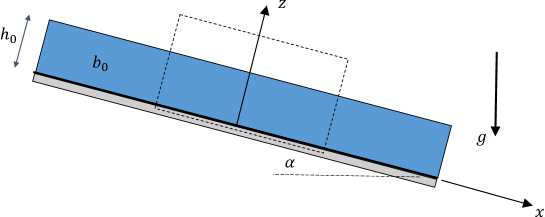
Figure 1: Schematic representation of the simulation setup.

The simulations comprise a temporal version of the classical inclined gravity current experiments of Ellison1959; Krug2013, as outlined in vanReeuwijk2017. Specifically, the problem entails a negatively buoyant (heavy) fluid layer of infinite extent flowing down a slope of angle $\alpha$, as shown schematically in figure 1. The dense fluid layer has an initial buoyancy $b_{0}<0$ and velocity $U_{0}$. Here, buoyancy is defined as $b=g(\rho_{a}-\rho)/\rho_{a}$ where $g$ is the gravitational acceleration and $\rho_{a}$ is the ambient density of the quiescent layer above the current. For an angle $\alpha=90^{o}$, this case represents a plane wall plume. In order to simulate this unbounded problem, a finite size domain is selected (dotted lines in Figure 1) and periodic boundary conditions are imposed on the lateral boundaries in the streamwise and spanwise directions. Because of the flow geometry and the periodic boundary conditions, the flow will remain statistically homogeneous in the $x$ and $y$ direction, and its statistics thus only depend on the wall-normal coordinate $z$ and time $t$ (see also Fedorovich2009). As noted in §1, this geometry removes any ‘head’ dynamics of the gravity current, and focusses exclusively on the shear-induced entrainment of ambient fluid at the top of the current. At the bottom wall, a no-flux (Neumann) boundary condition is enforced for buoyancy. For velocity, both no-slip and free-slip conditions will be considered.

The difference between a temporal and a spatial gravity current is that in the former the problem is spatially homogeneous and evolves in time, whilst in the latter, the problem is spatially inhomogeneous but steady in time. This has implications for the entrainment behaviour and the average position of the turbulent-nonturbulent interface (TNTI). In the temporal case, the TNTI’s average position evolves in time and the mean velocity through the TNTI is zero. In the spatial case, the TNTI’s average position is fixed and there is a mean velocity through the TNTI. However, these two problems are dynamically very similar as the physics of turbulent entrainment is governed by the difference between the TNTI velocity and the flow velocity (DaSilva2014).

The characteristic velocity scale, layer thickness and buoyancy, $u_{T}$, $h$, and $b_{T}$, respectively, are defined as

$$u_{T}h=\int_{0}^{\infty}\overline{u}\textnormal{d}z,\quad\quad u_{T}^{2}h=\int_{0}^{\infty}\overline{u}^{2}\textnormal{d}z,\quad\quad b_{T}h=\int_{0}^{\infty}\overline{b}\textnormal{d}z,$$ (4)

where the overline denotes averaging over the (homogeneous) $x$ and $y$ directions. We note that the integral buoyancy forcing $B_{0}$, defined as

$$B_{0}=-b_{T}h\sin\alpha=-b_{0}h_{0}\sin\alpha,$$ (5)

is a positive conserved quantity for this flow, and that $h$, $u_{T}$ and $b_{T}$ are expected to scale as $h\sim B_{0}^{1/2}t$, $u_{T}\sim B_{0}^{1/2}$, $b_{T}\sim B_{0}^{1/2}t^{-1}$ (vanReeuwijk2017). The flow cases were designed such that $B_{0}$ was identical for all angles; this ensures that the integral forcing in the streamwise momentum equation is identical for all flow cases considered, thus clearly bringing out any differences in the turbulence structure. Here, we are interested in flows where the turbulence (and associated mixing and entrainment) are driven purely by buoyancy effects, and so we are interested in how the flow dynamics vary as $\alpha$ varies, and in particular as it approaches small, yet crucially always finite, values. Since we have chosen to keep $B_{0}$ constant across all cases, our formulation does not allow for the consideration of $\alpha=0$ precisely. However, we aim to identify scalings as $\alpha$ takes very small values, in particular to understand the properties of the turbulence, entrainment and mixing in that limit. It is also important to remember at such shallow angles other physical processes, such as large-scale pressure gradients, hydraulic controls, or indeed substantial bottom roughness, are likely to be much more significant in determining the flow dynamics in geophysically-relevant situations. Here, we are focussed on understanding the properties of buoyancy-driven shear-induced turbulence in such temporal gravity currents.

The simulations are carried out with the direct numerical simulation code SPARKLE, which solves the Navier-Stokes equations in the Boussinesq approximation and is fully parallelised making use of domain decomposition in two directions. The spatial differential operators are discretised using second order symmetry-preserving central differences (Verstappen2003), and time-integration is carried out with an adaptive second order Adams-Bashforth method (vanReeuwijk2008a). Periodic boundary conditions are applied for the lateral directions.

The (bulk) Reynolds number Re and bulk Richardson number Ri are defined as

$$\textit{Re}=\frac{u_{T}h_{0}}{\nu},\quad\quad\textit{Ri}=-\frac{b_{T}h\cos\alpha}{u_{T}^{2}},$$ (6)

Consistent with (vanReeuwijk2017; Krug2017), the simulations were performed at $\Pr=1$ and initial Reynolds number $\textit{Re}_{0}=U_{0}h_{0}/\nu=3890$ on a large domain of $20h_{0}\times 20h_{0}\times 10h_{0}$ to ensure reliable statistics for this transient problem. A resolution of $N_{x}\times N_{y}\times N_{z}=1536^{2}\times 1152$, sufficient for (fully three-dimensional) direct numerical simulation, is employed for all simulations.

Table 1: Simulation data. Simulation domain for all simulations is $20h_{0}\times 20h_{0}\times 10h_{0}$ at a resolution of $1536^{2}\times 1152$. NS, FS: no-slip and free-slip velocity boundary conditions, respectively.

Sim.	$\alpha$	BC	$\textit{Re}_{0}$	$\textit{Ri}_{0}$	$t_{run}/t^{\star}$	$t_{stat}/t^{\star}$	$\textit{Re}_{b}$	$\textit{Re}_{\lambda}$	$\Delta x/\eta_{K}$
S2	2	FS	3890	0.50	55	10	308	75	1.47
S5	5	FS	3890	0.20	40	12	687	99	1.41
S10	10	FS	3890	0.10	40	12	1276	131	1.16
S10N	10	NS	3815	0.10	40	12	1019	78	1.18
S25	25	FS	3890	0.04	25	4	2132	145	1.06
S45	45	FS	3890	0.02	20	6	5437	152	1.09
S90	90	FS	3890	0.00	20	6	$\infty$	166	1.08

Further simulation details can be found in table 1. The simulations were performed for a duration $t_{run}$ and statistics were calculated over an interval $t_{stat}$ at the end of the simulation. Interestingly, over this period the flow is fully self-similar, and the profiles of $\overline{u}$ and $\overline{b}$ are very close to linear in $z$ (vanReeuwijk2017), consistent with laboratory experiments (Odier2009; Krug2015; Odier2014). The typical time scale is defined as $t^{*}=h_{0}/\sqrt{B_{0}}$. The grid is chosen such that $\Delta x/\eta_{K}<1.5$ for all flow cases. Here $\eta_{K}=(\nu^{3}/\varepsilon_{T})^{1/4}$ is the Kolmogorov lengthscale where $\varepsilon_{T}\equiv h^{-1}\int\varepsilon\textnormal{d}z$ is the characteristic dissipation rate. Also shown in table 1 are the buoyancy Reynolds number $\textit{Re}_{b}$ and Taylor Reynolds number $\textit{Re}_{\lambda}$, defined as

$$\textit{Re}_{b}=\frac{\varepsilon_{T}}{\nu\hat{N}^{2}},\quad\quad\textit{Re}_{\lambda}=\frac{u^{\prime}_{T}\lambda_{T}}{\nu}.$$ (7)

Here $N^{2}=\textnormal{d}\overline{b}/\textnormal{d}z\cos\alpha$ is the square buoyancy frequency where $(\hat{\cdot})$ denotes averaging over the ‘outer layer’ interval $z/h\in[1/2,1]$, $\lambda_{T}=\sqrt{10\nu e_{T}/\varepsilon_{T}}$ is the Taylor length scale and $u^{\prime}_{T}=\sqrt{2e_{T}/3}$ where $e_{T}\equiv h^{-1}\int e\textnormal{d}z$ is the characteristic turbulence kinetic energy (Tennekes1972, pp. 67-68). Both $\textit{Re}_{b}$ and $\textit{Re}_{\lambda}$ become constant as a function of time, and the values presented here are the typical values once a fully self-similar flow evolution is established. For an impression of the flow field and a characterisation of the turbulent-nonturbulent interface, see Krug2017.

3 Self-similarity and measures of mixing

3.1 Dependence on boundary conditions

Before considering all the cases, we first focus on the mixing behaviour for $\alpha=10^{o}$ and examine the differences between no-slip boundary conditions (simulation S10N) and free-slip boundary conditions (S10). In particular, we will demonstrate: 1) that the outer layer behaviours of S10 and S10N are practically indistinguishable with respect to their mixing behaviour; and 2) that the mixing characteristics are practically uniform in the outer layer of the flow – something which seems to be a unique feature of temporal gravity currents.

It is clear that free-slip boundaries do not occur in nature, but if the entrainment between the current and the ambient fluid is dominated by outer (effectively shear-driven) processes, the influence of velocity boundary conditions should be small. We do not address here the important question of the interplay between turbulence generated by bottom roughness and turbulence generated by shear-driven processes at the interface between the current and ambient (see Wells2010 for further discussion), or indeed driving mechanisms of a current other than the buoyancy force associated with a finite (albeit potentially exceptionally small) slope angle.

The evolution of $h$ and Ri are shown in figures 2(a,b). The layer thickness $h$ grows a little faster for S10 than for S10N, indicating, perhaps unsurprisingly, slightly higher entrainment for flows with no-slip boundary conditions. The evolution of Ri in time shows an initial growth to a maximum, after which Ri reduces monotonically and approaches a steady state for $t/t^{*}>30$; the final value of Ri is once again slightly higher for simulation S10N than for simulation S10.

The approach to a constant value of Ri is qualitatively similar to the behaviour observed for turbulent plumes, where plumes attain a constant value of the appropriately defined Ri far away from the source, i.e. they attain ‘pure plume balance’. If the flow has an excess of momentum at the source the plume is referred to as being forced (Morton1973), while if it has a deficiency of momentum flux it is referred to as being lazy (Hunt2001), although it has also been interpreted in a geophysical context as rising from a too large or ‘distributed’ source (Caulfield1995). In either case, the pure plume balance solution is a global attractor in an unstratified ambient (Caulfield1998), and the flow inevitably adjusts itself due to the work done by gravity until it attains pure plume balance. Restricting attention to $t/t_{*}>7$ (when the flow has transitioned to turbulence), the gravity current is ‘lazy’, approaching ‘pure’ behaviour for $t/t^{*}$ greater than (approximately) 30.

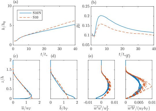
Figure 2: Time variation of: a) layer thickness $h$; and bulk Richardson number Ri, as defined in (6). Scaled wall-normal variation of scaled and spatially-averaged: c) $\overline{u}$; d) $\overline{b}$; e) $\overline{u^{\prime}w^{\prime}}$; and f) $\overline{w^{\prime}b^{\prime}}$ at time intervals $t/t_{*}=0.7$. Note that the multiple profiles for $\overline{u}$ and $\overline{b}$ show strong self-similarity, are approximately linear in particular away from the wall, and extend beyond $z/h=1$. Results for simulations S10N and S10 are shown with solid blue and dashed red lines respectively.

The (strong) self-similarity of the spatially-averaged velocity $\overline{u}$ and buoyancy $\overline{b}$ profiles are shown in figures 2(c,d), although, unsurprisingly, the solutions are very different near the wall in the ‘inner layer’. In particular, the ‘toe’ observed in the buoyancy profile for S10N is caused by the fact that the turbulence shear production $P_{S}$ defined as

$$P_{S}=-\overline{w^{\prime}u^{\prime}}\frac{\partial\overline{u}}{\partial z},$$ (8)

is zero at the velocity maximum and that as a consequence turbulence levels are low. This implies that buoyancy is ‘trapped’ near the (smooth) wall for flows with no-slip boundary conditions, an effect reported by Ellison1959. Importantly though, the flow profiles sufficiently far from the wall are very similar for the two simulations. Figures 2(e,f) show the wall normal transport of the streamwise momentum and buoyancy, respectively. It is apparent that there is a large negative momentum flux for simulation S10N, associated with the particular near wall dynamics in the inner layer, and in general, the free-slip fluxes are slightly larger than the no-slip fluxes, while there is not such a strong collapse as for the $\overline{u}$ and $\overline{b}$ profiles.

The fundamental budget of interest for mixing is the budget of turbulence kinetic energy $e$, which for the temporal gravity current is given by

$$\frac{\partial e}{\partial t}=\underbrace{-\overline{w^{\prime}u^{\prime}}\frac{\partial\overline{u}}{\partial z}}_{P_{S}}\ \ \underbrace{-\overline{u^{\prime}b^{\prime}}\sin\alpha+\overline{w^{\prime}b^{\prime}}\cos\alpha}_{P_{B}}-\varepsilon.$$ (9)

where $P_{S}$ is the shear production and $P_{B}$ is the buoyancy production of turbulent kinetic energy with dissipation rate $\varepsilon=\nu\overline{(\partial u_{i}^{\prime}/\partial x_{j})^{2}}$. Since we are considering a flow upon a slope, there is a choice to be made as to the definition of the important mixing parameters known as the flux Richardson number $\textit{Ri}_{f}$, the turbulent flux coefficient $\Gamma$ (osborn80) and the gradient Richardson number $\textit{Ri}_{g}$. We define these quantities as follows:

$$\quad\textit{Ri}_{f}(z,t)=\frac{-P_{B}}{P_{S}},\quad\quad\Gamma(z,t)=\frac{-P_{B}}{\varepsilon},\quad\quad\textit{Ri}_{g}(z,t)=\frac{{\partial\overline{b}}/{\partial z}\cos\alpha}{\left({\partial\overline{u}}/{\partial z}\right)^{2}}.$$ (10)

For the gradient Richardson number $\textit{Ri}_{g}$ we have chosen to use the component of the density gradient in the direction of gravity in the numerator, which is a self-consistent generalisation of the conventional interpretation of a gradient Richardson number as a quantification of the relative importance of destabilising shear to stabilising density gradients.

For the two (potentially related) flux quantities $\textit{Ri}_{f}$ and $\Gamma$ we have chosen to use the full buoyancy production of turbulent kinetic energy, which for non-zero $\alpha$ (as always considered here) has in general a non-zero along-slope component. This choice means that the energy-based interpretation of these terms must be done with care, particularly for larger values of $\alpha$. Indeed, for sufficiently steep angles, it is to be expected that the buoyancy production term will change sign and become negative as the dense flow down the slope will actually lead to an increase in the turbulent kinetic energy, rather than a decrease (ultimately due to an exchange into the potential energy reservoir). It is important to appreciate that the quantities in (10) are in general functions of $z$ and $t$, involving as they do only horizontal averages, and so there is not necessarily a simple way to relate $\Gamma$ and $\textit{Ri}_{f}$, or indeed to compare with other studies of related flows, such as the experimental flows with the same slope angle discussed in Odier2014. (See Wells2010 for a further discussion of this subtle, and often not appreciated point.)

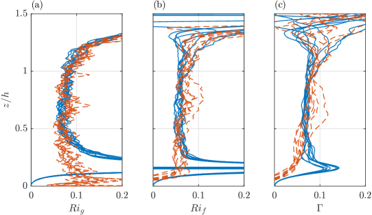
Figure 3: Scaled wall-normal variation (over time interval documented in Table 1) of: (a) Gradient Richardson number $\textit{Ri}_{g}$; (b) Flux Richardson number $\textit{Ri}_{f}$; and (c) turbulent flux coefficient $\Gamma$ as defined in (10) for simulation S10N (red lines) and simulation S10 (blue lines).

For the temporal gravity current, both the mean and turbulence kinetic energy are expected to scale with $B_{0}$ and are therefore independent of time in the fully self-similar regime. The turbulence kinetic energy budget will then be in a statistically steady state, and thus the two production terms when appropriately integrated in the wall-normal direction must balance the wall-normal-integrated dissipation rate:

$$\mathcal{P}_{S}+\mathcal{P}_{B}=\mathcal{E}$$ (11)

Here, the caligraphic scripts denote quantities integrated over the wall-normal direction, i.e. $\mathcal{P}_{S}=\int_{0}^{\infty}P_{S}\textnormal{d}z$, $\mathcal{P}_{B}=\int_{0}^{\infty}P_{B}\textnormal{d}z$ and $\mathcal{E}=\int_{0}^{\infty}\varepsilon\textnormal{d}z$. Note that this implies that

$$\langle\textit{Ri}_{f}\rangle\simeq\frac{\langle\Gamma\rangle}{1+\langle\Gamma\rangle},$$ (12)

where the angle brackets denote quantities calculated from the integral properties. The quantity $\langle\textit{Ri}_{f}\rangle$ quantifies the proportion of the energy injected into the flow which has led to increases in the potential energy through irreversible mixing processes, and $\mathcal{P}_{B}$ is expected to be a sink of kinetic energy ultimately leading to an increase in the flow potential energy, although particularly for flows where the Boussinesq approximation does not apply, the energy pathways are more convoluted (see Tailleux2013; Scotti2015, for detailed discussions). Understanding and parameterising such partitioning is a central challenge in oceanography (see Ivey2008; Ferrari2009, for reviews).

It is apparent from figure 3 that the values of these three quantities are quite similar for the two simulations with different wall boundary conditions yet small angle $\alpha=10^{\circ}$, except in the near wall inner layer $z/h\lesssim 0.3$, and indeed are quite close to constant over $0.3<z/h<1.0$. The evidently self-similar (and essentially linear) distributions of $\overline{u}$ and $\overline{b}$ naturally lead to constant values of the gradient Richardson number $Ri_{g}$ over much of the (self-similar) depth of the current. The perhaps more surprising observation is that the flux Richardson number $\textit{Ri}_{f}$ and the (apparently related) turbulent flux coefficient $\Gamma$ are close to constant across the interior of the current for $0.3<z/h<1.0$. Indeed, although as already noted there is no necessity for the simple relationship in (12) to hold, $\Gamma$ is indeed slightly more than $Ri_{f}$.

There is no immediately obvious reason why $\textit{Ri}_{f}(z,t)$ (and $\Gamma(z,t)$) should be approximately constant and similar to $\textit{Ri}_{g}(z,t)$, but it is entirely consistent with the behaviour of the flows in stratified plane Couette flow, where Deusebio2015 found a close to linear relationship between appropriate definitions of a gradient Richardson number and flux Richardson number, which applies at all heights within the flow. Furthermore, this is also evidence (as discussed further below) that the turbulent Prandtl number for this flow is an $O(1)$ constant. The turbulent diffusivities for momentum and buoyancy, (once again in general functions of $z$ and $t$) and the associated turbulent Prandtl number are defined as

$$K_{m}=-\overline{w^{\prime}u^{\prime}}\left(\frac{\partial\overline{u}}{\partial z}\right)^{-1},\quad K_{\rho}=-\overline{w^{\prime}b^{\prime}}\left(\frac{\partial\overline{b}}{\partial z}\right)^{-1},\quad Pr_{T}=\frac{K_{m}}{K_{\rho}},$$ (13)

and so it is straightforward to establish that

$$\textit{Ri}_{f}=\frac{\textit{Ri}_{g}}{Pr_{T}}\left[1-\frac{\overline{u^{\prime}b^{\prime}}}{\overline{w^{\prime}b^{\prime}}}\tan\alpha\right].$$ (14)

Since the angle $\alpha$ is relatively small, the term in the square bracket is close to unity and so the observation that the flux Richardson number $\textit{Ri}_{f}$ is close to constant and similar in magnitude to the constant gradient Richardson number $\textit{Ri}_{g}$ implies that $Pr_{T}\sim O(1)$ and close to constant (with $z$ and $t$). We observe that for all heights in the current sufficiently far away from the wall, the flow ‘chooses’ a balanced coupled configuration for which $\textit{Ri}_{f}$ and $\Gamma$ are constant across the outer layer. This inherently emergent dynamical behaviour of spatially-constant $\textit{Ri}_{f}$ and $\Gamma$ occurs for all simulations, although $\textit{Ri}_{f}$ and $\Gamma$ do have a non-trivial dependency on $\alpha$ as discussed further below, not least because of the increasing influence of the along-slope term in $P_{B}$ as the slope angle increases.

3.2 Dependence on the slope angle

Having established that the boundary conditions have relatively limited influence on turbulent entrainment, at least for such purely buoyancy-driven down-slope gravity currents, we restrict attention to free-slip velocity boundary conditions so that by construction we can focus on outer layer dynamics. We consider simulations with a wide variety of angles $\alpha$ between 2 and 90 degrees. It is important to appreciate that the simulation with $\alpha=90^{\circ}$ closely resembles the flow of a temporal plume, and is in a very real sense a qualitatively different flow than a temporal gravity current.

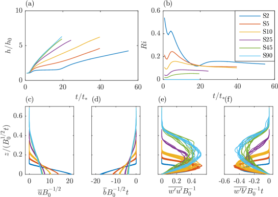
Figure 4: Properties of the results of free-slip simulations for a range of slope angles, as marked with different line types. Time variation of: (a) $h$; and (b) Ri. Scaled wall-normal variation of spatially-averaged: (c) $\overline{u}$; (d) $\overline{b}$; (e) $\overline{u^{\prime}w^{\prime}}$; and (f) $\overline{w^{\prime}b^{\prime}}$ over the time interval documented in Table 1.

Figure 4(a) shows the time evolution of the current depth $h$ for simulations with a range of angles, showing that the depth grows approximately linearly with time as expected. It is also clear that $h$ grows more rapidly as the angle $\alpha$ is increased. As shown in figure 4(b), the bulk Richardson number Ri approaches a constant value once the flow is self-similar, with the asymptotic value decreasing with increasing angle.

The extents of the self-similarity of various spatially-averaged characteristics of the flows are shown in figures 4(c-f). In contrast to figure 2, $B_{0}$ and $t$ are used to scale both the wall-normal coordinate and the various flow characteristics instead of $u_{T}$ and $b_{T}$, so that it is possible to identify the differences in absolute amplitudes between simulations with relatively small angles (i.e. $\alpha=2^{\circ},5^{\circ},10^{\circ}$) and relatively larger angles (i.e. $\alpha=25^{\circ},45^{\circ},90^{\circ}$). Clearly, the currents from simulations with relatively low angles are shallower and have higher amplitudes of $\overline{u}$ and $\overline{b}$ compared to the currents along relatively steeper slopes. Flows along slopes with small $\alpha$ require more work to be done for an increase in potential energy, and so the flow will accelerate until this can be achieved, and the self-similarity is at least approximately achieved. As is apparent in figures 4(e,f), the turbulent fluxes are also close to self-similar, and it is striking that the maximum amplitude is similar for all values of $\alpha$, although the location of the maximum does depend on $\alpha$, with the maximum being closer to the wall for flows with smaller slope angle $\alpha$.

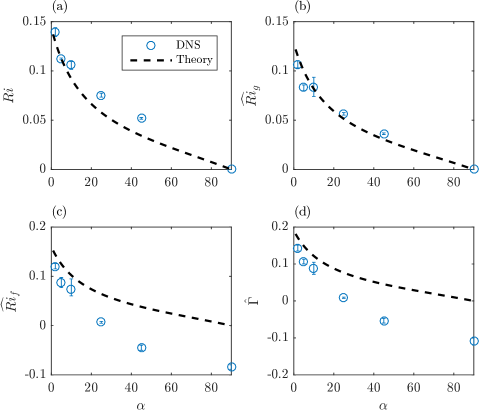
Figure 5: Variation with slope angle $\alpha$ of the numerical data (marked with circles) and theoretical predictions (marked with dashed lines) for: (a) Ri, modelled by (35); (b) $\widehat{\textit{Ri}_{g}}$, modelled by (35); (c) $\hat{\textit{Ri}_{f}}$, modelled by (36); and (d) $\hat{\Gamma}$, modelled by (36). A hat denotes an average over the outer layer interval $z/h=[1/2,1]$.

In Figure 5, the observed dependence of the mixing parameters on the slope angle $\alpha$ is presented by circles. Here, the hatted quantities denote average values over the outer layer interval $z/h=[1/2,1]$ (see Figure 3). The error bars show the difference between the largest and smallest value within the time window $t_{stat}$ over which statistics were gathered (the statistics were gathered at intervals $t/t_{*}=0.7$). Shown with the dashed line are results from a theoretical model which will be introduced in §4.2. Clearly, all indicators display similar behaviour in the sense that their values increase as the slope angle reduces. Importantly, though, the values remain bounded and well below the critical linear stability threshold of $\textit{Ri}=1/4$. $\widehat{Ri}_{f}$ and $\hat{\Gamma}$ are positive only for the three low-angle (but still finite slope) cases. For $\alpha>25^{o}$, the along-slope turbulence kinetic energy contribution of $P_{B}$ becomes larger than the perpendicular contribution, and thus both $\widehat{Ri}_{f}$ and $\hat{\Gamma}$ will become negative. As already discussed, in such a regime, the flux Richardson number $\textit{Ri}_{f}$ and the turbulent flux coefficient $\Gamma$ are not appropriately defined.

3.3 Turbulent entrainment

Turbulent entrainment, as quantified by the entrainment parameter (vanReeuwijk2017)

$$E=\frac{1}{u_{T}}\frac{\textnormal{d}h}{\textnormal{d}t},$$ (15)

is naturally closely related to turbulent mixing. In figure 6(a), we plot the temporal variation of $E$ for all six simulations. Clearly, $E$ increases with $\alpha$. Since $\alpha$ is directly related to the bulk Richardson number Ri through its definition (6), this relationship suggests, analogously to the classic parameterisation of Ellison & Turner discussed in §1, that $E$ has a functional dependence on Ri. Despite keeping $B_{0}$ the same for all simulations, quantifying $E$ in the simulations at the smallest (yet crucially still finite, as noted above) angles is challenging since there is a lower turbulence intensity (not shown) as a result of the (relatively) stronger stratification. This is particularly evident in the data extracted from simulation S2, in which the flow almost completely relaminarises after the initial burst associated with Kelvin-Helmholtz-like shear instabilities as the flow accelerates from its initial condition. However, the very low, but inherently transient, level of turbulence (evident for $t/t_{*}\simeq 10$) implies that the fluid layer will accelerate due to the low level of dissipation until a second transition occurs after which ‘pure’ behaviour emerges for $t/t_{*}>40$. This second transition appears to lead to a quasi-stationary turbulent state. Therefore, it is not appropriate to interpret this flow as exhibiting ‘intermittent’ turbulence, but rather that our chosen initial conditions are in some sense imbalanced, and so there is a relatively long initial transient evolution, exhibiting non-monotonic turbulence intensity, until the flow self-organises into its eventual quasi-stationary turbulent state.

The entrainment law $E(\textit{Ri})$ is shown in the bottom plot of figure 6, together with the Ellison and Turner entrainment law defined in (1). Here, Ri is the value associated with the ‘pure’ gravity current after initial transients have decayed, and the velocity and buoyancy distributions have evolved into the clearly coupled (and close to linear) distributions as shown in figure 4(c). Precisely, the value of $E$ was calculated by averaging over the interval $t_{stat}$ (table 1), and the horizontal and vertical error bars denote the maximum and minimum observed values of Ri and $E$ over this time interval.

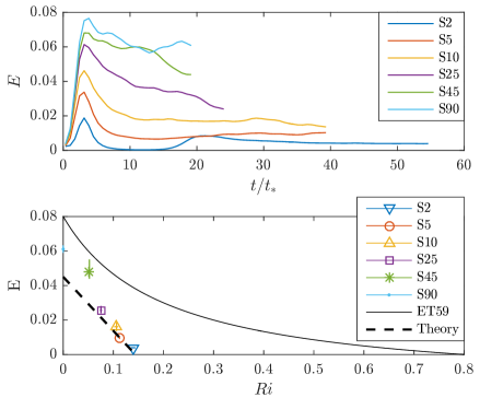
Figure 6: (a) Variation with time of the entrainment parameter $E$ as defined in (15) for various simulations, plotted with different line types. (b) Variation with Ri of the averaged entrainment parameter $E$ as defined in (15) for various simulations, plotted with different symbols. The classical empirical parameterisation ET59 as defined in (1) is plotted with a solid line, while the new proposed parameterisation (16) is plotted with a dashed line.

Interestingly, Ri remains constrained between $0<\textit{Ri}<0.2$ for all angles. Crucially, when defined in this way, we observe that it is impossible to reach the higher values of Ri observed in the Ellison1959 experiments: the coupled velocity and buoyancy distributions inevitably force the Richardson number to be bounded above by $0.2$ when there is any observable turbulence at all, consistently with the recent observations of Deusebio2015 and Zhou2017 in plane Couette flow. Furthermore, the values of $E$ as quantified from our numerical simulations are lower than those reported experimentally by Ellison1959 and Odier2014 although direct quantitative comparison is challenging, not least due to the different forcing mechanisms of the different flows.

Of course, the spatially evolving experimental flow geometry is qualitatively different from the inherently temporal flow geometry considered here. It is also at least plausible that the gravity current in their experiments was not yet ‘pure’ in a statistically steady state, which would go some way to explain their higher observed values for Ri and $E$. Furthermore, as noted in §1, it is also conceivable that their experimental data were contaminated by end-effect mixing at a ‘head’ being swept back along the current, as such mixing is expected to be substantially stronger, as investigated in detail by Sher2015. Whatever the reason for the mismatch, it is apparent that there is a marked decrease in $E$ with Ri, and there is a clear ‘switch-off’ of entrainment (quantified in this way) at a maximum value of Ri.

Focusing on the simulations S2, S5 and S10 with relatively small slope angles, (where the buoyancy production $P_{b}<0$, and so the expected sink of turbulent kinetic energy due to mixing occurs) the entrainment law can be reasonably well approximated by a linear relation of the form

$$E=a(\textit{Ri}_{\max}-\textit{Ri});\ a=0.31,\ \textit{Ri}_{\max}=0.15,$$ (16)

as marked in figure 6(b) by the dashed line. We present a detailed theoretical justification for this model in §4.2, but we once again stress that for these simulations, the mean velocity and buoyancy profile are both close to linear and appear to be coupled in a way which strongly suggests that there is a maximum value of Ri beyond which turbulence cannot be sustained, at least in the flows considered here, purely driven by buoyancy forces down slopes of small (but still finite) angle.

4 Model development

4.1 Turbulence parameterisation

As demonstrated in Krug2017, the vertical length scale is proportional to $\hat{e}^{1/2}/\hat{S}$, which implies that the turbulence is ‘shear-dominated’ (Mater2014). It is thus natural to investigate whether a turbulence parameterisation can be constructed using the strain rate $S=|\partial\overline{u}/\partial z|$ and the turbulence kinetic energy $e$ to scale the eddy diffusivity calculated from three simulations with relatively small slope angles, i.e. the simulations S2, S5 and S10. For the turbulent diffusivities defined in (13), this suggests that

$$K_{m}=c_{m}e/S,\quad\quad K_{\rho}=c_{\rho}e/S.$$ (17)

In figure 7(a), we plot $K_{m}S/e$ for all three small-slope simulations as a function of $z/h$ at a range of times. The vertical dashed line shows $c_{m}=0.25$, demonstrating that this parameterisation is an excellent fit for a wide range of times for all three simulations, particularly sufficiently far away from the wall, i.e. $0.3<z/h<1$. Conversely, in figure 7(d) by plotting $K_{m}/(u_{T}h)$, we demonstrate that there is no collapse when scaled with the similarity variables. Similarly, for the turbulent scalar diffusion $K_{\rho}$, we observe a collapse upon plotting $K_{\rho}S/e$, as shown in figure 7(b), with an approximately constant value sufficiently far away from the wall of $c_{\rho}=0.31$ (as plotted with a vertical dashed line). This implies that for three lowest angle cases, the turbulent Prandtl number $\Pr_{T}=K_{m}/K_{\rho}=c_{m}/c_{\rho}=0.8$ independent of the flow angle, thus clearly suggesting that $Pr_{T}$ remains finite, and indeed is of $O(1)$. Once more there is no collapse upon scaling $K_{m}$ by $u_{T}h$, as shown in figure 7(e).

Similarly, we predict that the dissipation rate $\varepsilon$ can also be scaled appropriately with $e$ and the strain rate $S$, which on dimensional grounds implies that

$$\varepsilon=c_{\varepsilon}eS,$$ (18)

for some constant $c_{\varepsilon}$. We plot $\varepsilon/(eS)$ in figure 7(c), and once again there is a clear collapse, with an approximate value of $c_{\varepsilon}=0.21$ away from the immediate vicinity of the wall, as marked on the figure with a dashed line. Conversely, as shown in figure 7(f), there is no collapse of $\varepsilon$ when scaling with $u_{T}^{3}/h$.

It is also interesting to note, using the definitions of $\textit{Ri}_{f}$, $\Gamma$, $P_{S}$ (10), and $K_{m}$ (13), as well as the (verified) parameterisation (17), that

$$\varepsilon=\left(\frac{\textit{Ri}_{f}}{\Gamma}\right)P_{S}=\left(\frac{\textit{Ri}_{f}}{\Gamma}\right)K_{m}S^{2}\quad\Rightarrow\quad\varepsilon=\underbrace{\left(\frac{\widehat{\textit{Ri}}_{f}}{\hat{\Gamma}}\right)c_{m}}_{c_{\varepsilon}}eS.$$ (19)

Comparing this relationship to the empirical observation that $c_{\varepsilon}=0.21$ and $c_{m}=0.25$, this suggests $\widehat{\textit{Ri}}_{f}/\hat{\Gamma}=0.84$ and thus that $\widehat{\textit{Ri}}_{f}<\hat{\Gamma}$, consistently with (12).

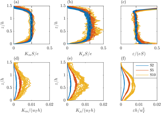
Figure 7: Variation with scaled height $z/h$ for the three simulations S2 (blue lines), S5 (red lines) and S10 (yellow lines) at several time instants (see Table 1 for time interval) for: (a) $K_{m}S/e$; (b) $K_{\rho}S/e$; (c) $\varepsilon/(eS)$; (d) $K_{m}/(u_{T}h)$; (e) $K_{\rho}/(u_{T}h)$; (f) $\varepsilon h/u_{T}^{3}$. In panels (a-c) there is clear collapse, and the relevant empirical constants of proportionality $c_{m}=0.25$, $c_{\rho}=0.31$ and $c_{\varepsilon}=0.21$ are marked with vertical dashed lines.

It is apparent that for the key properties of the turbulence in this flow, the appropriate scalings are not based around the conventional integral velocity scale $u_{T}$ and $h$. This is clearly demonstrated in figure 8(a), where $u_{T}$ and $e_{T}^{1/2}$ are displayed as a function of the slope angle $\alpha$. As mentioned earlier, these quantities are both expected (and observed) to scale according to $B_{0}^{1/2}$ in the self-similar regime. It is striking that $e_{T}$ is virtually independent of $\alpha$, but $u_{T}$ increases dramatically as the slope angle reduces. Indeed, the structure of the $u_{T}$ variation is consistent with $u_{T}$ diverging as $\alpha\rightarrow 0$. As is apparent from the definition (5) of the integral forcing $B_{0}$, the forcing buoyancy $b_{0}h_{0}$ must diverge as $\alpha\rightarrow 0$ to ensure the distinguished limit that $B_{0}$ remains constant, and so it is perhaps unsurprising that $u_{T}$ becomes very large as $\alpha$ approaches small values. The physical picture that emerges is that the flows with higher Richardson numbers for lower slope angles $\alpha$ require higher shear (and thus higher $u_{T}$) to sustain a similar level of turbulence. This will be explained in detail by the conceptual model we develop in the next section. What will not be revealed by the model is why the turbulence level $e_{T}/B_{0}^{1/2}$ is virtually independent of $\alpha$. In figure 8(b), we plot the variation of $(3/2)(\overline{w^{\prime}w^{\prime}}/e)$ with slope angle $\alpha$ to quantify the extent of anisotropy within the flow. Unsurprisingly, due to the inherent greater magnitude of the streamwise velocity $u$, this quantity is always less than one, and exhibits only a slight dependence on angle when scaled in this way, decreasing slightly as $\alpha$ tends to small values, due naturally to the stabilising effect of stratification becoming somewhat more significant. However, there are no signs of a transition to strongly stratified turbulence, and this cannot be an explanation for the observation of $E\rightarrow 0$ as $\alpha$ tends towards zero.

In figure 8(c) and (d), we plot the variation with slope angle $\alpha$ of the three key terms $\mathcal{P}_{S}$, $4\mathcal{P}_{B}$ (the prefactor is included for visual purposes only) and $\mathcal{E}$ in the integral turbulent kinetic energy equation 11 and averaged over the time interval $t_{stat}$ (Table 1). In figure 8(c), the various terms are scaled using $(B_{0}^{3})^{-1/2}$, which reveals the appropriate and expected dynamics for small angles, showing that the actual production of turbulence increases. This can be understood from the fact that the velocity gradient is much larger (see figure 4) as the flow will keep accelerating until an essentially equilibrium state is attained. As mentioned earlier, the buoyancy production term $\mathcal{P}_{B}$ is negative for the smallest three angles and changes sign around $\alpha=20^{o}$, which can be understood in terms of the relative size of the two terms in $\mathcal{P}_{B}$ (9), with the contribution of the first (generally positive) term dominating for large $\alpha$ and the second (generally negative) term for small $\alpha$. Clearly, not least because of the opposing effects of these two terms, the main overall balance is between shear production $\mathcal{P}_{S}$ and dissipation $\mathcal{E}$, and $\mathcal{P}_{B}$ only makes a relatively small contribution to the overall budget.

Although it is apparent from figure 8(c) that the magnitude of the various key terms in the integral turbulent kinetic energy equation 11 increase as $\alpha$ decreases, their rate of increase is clearly significantly smaller than that exhibited by $u_{T}$ as shown in figure 8(a). Figure 8(d) shows once more the integral turbulence kinetic energy budget but this time scaled by $u_{T}^{3}$. Scaled in this way, as $\alpha\rightarrow 0$ the production of turbulent kinetic energy appears to go to zero, although it is more appropriate to interpret this figure as implying that the production of turbulent kinetic energy becomes effectively insignificant as $\alpha\rightarrow 0$. Significantly, even though $P_{B}$ increases in terms of $B_{0}$, the relative production tends to zero as $\alpha\rightarrow 0$. This has profound implications for the entrainment as there will be no energy available for turbulent mixing.

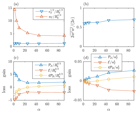
Figure 8: Variation with slope angle of (a) the characteristic velocities $u_{T}$ and turbulence $e_{T}^{1/2}$, (b) the anisotropy of the turbulence and (c,d) the vertically integrated terms in the turbulent kinetic energy equation: shear production $\mathcal{P}_{S}$ (marked with blue triangles); dissipation rate $\mathcal{E}$ (red inverted triangles); buoyancy production $4\mathcal{P}_{B}$ (yellow circles). In panel (c) these quantities are scaled with $(B_{0}^{3})^{1/2}$, while in panel (d) they are scaled with $u_{T}^{3}$.

4.2 An approximate integral model for small $\alpha$

Since we observe apparently coupled and essentially linear profiles of velocity and buoyancy, we now construct a model for entrainment based around this central observation, in an attempt to predict the apparent ‘switch-off’ of the entrainment, particularly for the simulations associated with a low slope angle. The conservation equations for mean momentum, buoyancy and turbulent kinetic energy are given by, respectively

$$\frac{\partial\overline{u}}{\partial t} =-\frac{\partial\overline{{w}^{\prime}{u}^{\prime}}}{\partial z}-\overline{b}\sin\alpha,$$ (20)

$$\frac{\partial\overline{b}}{\partial t} =-\frac{\partial\overline{{w}^{\prime}{b}^{\prime}}}{\partial z},$$ (21)

$$\frac{\partial e}{\partial t} =-\overline{w^{\prime}u^{\prime}}\frac{\partial\overline{u}}{\partial z}+\overline{w^{\prime}b^{\prime}}\cos\alpha-\varepsilon.$$ (22)

Here, we have neglected the term $\overline{u^{\prime}b^{\prime}}\sin\alpha$ describing the along-slope turbulent production by buoyancy in the turbulent kinetic energy equation. This limits the validity of the approximation to small values of $\alpha$, as we are interested in the dynamical behaviour of the system where the dominant effect of the buoyancy is to extract kinetic energy due to vertical mixing associated with entrainment. The system of equations is closed using our parameterisations of the eddy diffusivities of momentum and buoyancy, and the scaling of the dissipation rate in terms of the turbulent kinetic energy and the mean shear, i.e. (17) and (18).

Furthermore, since we observe that the profiles of $u$ and $b$ appear to be self-similar, we assume a solution of the form

$$\overline{u}=\underbrace{a_{u}B_{0}^{1/2}}_{u_{T}}f_{u}(\eta),\quad\quad\overline{b}=\underbrace{{-}a_{b}\frac{B_{0}}{h\sin\alpha}}_{b_{T}}f_{b}(\eta),\quad\quad e=\underbrace{a_{e}B_{0}}_{e_{T}}f_{e}(\eta)$$ (23)

where the scaled wall-normal distance $\eta=z/h$ is the natural similarity variable and $a_{u}$, $a_{b}$ and $a_{e}$ are coefficients that will need to be determined. Given the relative complexity of the equations we will not attempt to obtain closed-form solutions. Instead we employ the Von Karman-Pohlhausen method (Lighthill1950; Spalding1954; Schlichting2000) to construct an approximate solution to the system of coupled PDES using an ansatz

$$f_{u}=f_{b}=\frac{2}{\eta_{1}^{2}}(\eta_{1}-\eta),\quad\quad f_{e}=\frac{6\eta}{\eta_{1}^{3}}(\eta_{1}-\eta),$$ (24)

on the interval $\eta\in[0,\eta_{1}]$. These profiles are constructed such that $\int_{0}^{\infty}f_{u}\textnormal{d}\eta=\int_{0}^{\infty}f_{b}\textnormal{d}\eta=\int_{0}^{\infty}f_{e}\textnormal{d}\eta=1$ in order to enforce consistency with $u_{T}$, $b_{T}$ and $e_{T}$.

Using (23) and (24), the key integrals of the volume, momentum and buoyancy in the current take the forms

$$\int_{0}^{\infty}\overline{u}dz =B_{0}^{1/2}h\int_{0}^{\eta_{1}}f_{u}d\eta=a_{u}B_{0}^{1/2}h,$$ (25)

$$\int_{0}^{\infty}\overline{u}^{2}dz =B_{0}h\int_{0}^{\eta_{1}}f_{u}^{2}d\eta=\frac{4}{3}a_{u}^{2}B_{0}h,$$ (26)

$$\int_{0}^{\infty}\overline{b}\sin\alpha dz =-B_{0}\int_{0}^{\eta_{1}}f_{b}d\eta=-a_{b}B_{0}.$$ (27)

From the fact that the buoyancy integral is conserved and equal to $-B_{0}$, it follows directly that $a_{b}=1$. From the definition of $h$ (4), it follows that $\eta_{1}=4/3$. Making the further scaling assumption that $h=aB_{0}^{1/2}t$, for a further empirical constant $a$, we obtain the following expressions for the main quantities of interest:

$$u_{T} =\frac{M}{Q}=a_{u}B_{0}^{1/2}, E =\frac{1}{u_{T}}\frac{dh}{dt}=\frac{a}{a_{u}}$$ (28)

$$\hat{N}^{2} =\frac{\partial\overline{b}}{\partial z}\cos\alpha=\frac{9}{8}\frac{B_{0}}{h^{2}\tan\alpha}, \hat{S} =\left|\frac{\partial\overline{u}}{\partial z}\right|=\frac{9}{8}\frac{B_{0}^{1/2}a_{u}}{h},$$ (29)

Ri $$=-\frac{b_{T}h\cos\alpha}{u_{T}^{2}}=\frac{1}{a_{u}^{2}\tan\alpha}, \widehat{\textit{Ri}}_{g} =\frac{\hat{N}^{2}}{\hat{S}^{2}}=\frac{8}{9}\frac{1}{a_{u}^{2}\tan\alpha},$$ (30)

$$\widehat{\textit{Ri}}_{f} =\frac{8}{9}\frac{1}{a_{u}^{2}\Pr_{T}\tan\alpha}, \hat{\Gamma} =\frac{8}{9}\frac{c_{m}}{c_{\varepsilon}\Pr_{T}a_{u}^{2}\tan\alpha}.$$ (31)

Here, the hat emphasises that these quantities represent the expected average value in the outer layer.

Equations for the various empirical constants can be determined by integrating (20) and (22) from $\eta=0$ to $\eta=\eta_{1}$, leading ultimately to

$$aa_{u} =1,$$ (32)

$$\frac{9a_{u}}{8}(c_{m}-c_{\varepsilon})-\frac{c_{m}}{a_{u}\tan\alpha Pr_{T}} =a.$$ (33)

Analogous integration of the buoyancy equation (21) does not provide any further information, confirming that the chosen profiles are a priori consistent with (21). Solving for $a_{u}$ and $a^{2}$ results in

$$a_{u} =\frac{1}{a}, a^{2} =\frac{9}{8}\frac{Pr_{T}(c_{m}-c_{\varepsilon})\tan\alpha}{\tan\alpha\Pr_{T}+c_{m}}$$ (34)

Interestingly, the empirical constant $a_{e}$ remains free, implying that these results are not directly sensitive to the actual magnitude of the turbulent kinetic energy fluctuations.

For the mixing parameters, the model thus predicts that

Ri $$=\frac{9}{8}\frac{c_{m}-c_{\varepsilon}}{\tan\alpha+c_{\rho}}, \widehat{\textit{Ri}}_{g} =\frac{c_{m}-c_{\varepsilon}}{\tan\alpha+c_{\rho}},$$ (35)

$$\widehat{\textit{Ri}}_{f} =\frac{c_{m}-c_{\varepsilon}}{\tan\alpha\Pr_{T}+c_{m}}, \hat{\Gamma} =\frac{c_{m}}{c_{\varepsilon}}\frac{c_{m}-c_{\varepsilon}}{\tan\alpha\Pr_{T}+c_{m}}.$$ (36)

Note that these expressions are fully consistent with relations (14), (19) derived above in sections 3 and 4.1 respectively. Figure 5 shows how these theoretical predictions compare to the simulation data.

Both Ri and $\widehat{\textit{Ri}}_{g}$ compare well across the entire range of simulations, even – somewhat surprisingly – for the large angle cases. This suggests that the along-slope buoyancy production is not significant for these two parameters, although it also could just be a straightforward consequence of the fact that both Ri and $\hat{\textit{Ri}}_{f}$ tend to zero as $\alpha\rightarrow 90^{o}$. Conversely, $\widehat{\textit{Ri}}_{f}$ and $\hat{\Gamma}$ only really compare well to the numerical simulation data for the three relatively low-angle cases. For $\alpha>25^{o}$, the theoretical and numerically simulated values start deviating strongly, due presumably to the omission of the along-slope turbulent kinetic energy production due to buoyancy, as is clear from the fact that both quantities change sign for the numerical simulation data. As already discussed, in such a regime, the flux Richardson number $\textit{Ri}_{f}$ and the turbulent flux coefficent $\Gamma$ are not appropriately defined.

The model predicts that the maximal attainable values for the mixing parameters occur as $\alpha\rightarrow 0$ and are given by

$$\textit{Ri}_{\max} =\frac{9}{8}\frac{c_{m}-c_{\varepsilon}}{c_{\rho}}\approx 0.15, \widehat{\textit{Ri}}_{g;\max} =\frac{c_{m}-c_{\varepsilon}}{c_{\rho}}\approx 0.13,$$ (37)

$$\widehat{\textit{Ri}}_{f;\max} =\frac{c_{m}-c_{\varepsilon}}{c_{m}}\approx 0.16, \hat{\Gamma}_{\max} =\frac{c_{m}-c_{\varepsilon}}{c_{\varepsilon}}\approx 0.19.$$ (38)

The entrainment parameter $E=a^{2}$, and the angle $\alpha$ will need to be eliminated in order to obtain the entrainment law. This can be achieved by using the equation for Ri in (35), which can be rearranged to yield

$$\tan\alpha=\frac{9}{8}\frac{c_{m}-c_{\varepsilon}}{\textit{Ri}}-\frac{c_{m}}{\Pr_{T}}.$$ (39)

Substituting this relationship into the expression for $a^{2}$ (34), it follows that the entrainment parameter $E$ is given by

$$E=\frac{c_{m}}{\Pr_{T}}(\textit{Ri}_{\max}-\textit{Ri}).$$ (40)

Using the empirically determined values $c_{\varepsilon}=0.21$, $c_{m}=0.25$ and $\Pr_{T}=0.8$, we find that

$$E=0.31(\textit{Ri}_{\max}-\textit{Ri}),\quad\quad\textit{Ri}_{\max}=0.15.$$ (41)

Interestingly, this entrainment prediction is in very good agreement with the simulation results for the low angle cases as is clear from figure 6(b), strongly suggesting that this model is appropriate, and that there is indeed a (particular kind of) ‘switch-off’ of entrainment in these flows for sufficiently large Ri. Crucially, this particular ‘switch-off’ is not associated with a suppression of the turbulence: for all cases, the turbulence levels $e_{T}$ were similar, and finite. Rather it is the scaled intensity of the turbulence $e_{T}^{1/2}/u_{T}$ which tends to zero as $\textit{Ri}\rightarrow\textit{Ri}_{\max}$. This key phenomenology is captured by the theoretical model, which predicts that for $\alpha\ll 1$, $e_{T}\sim B_{0}$ and $u_{T}\sim B_{0}^{1/2}\alpha^{-1/2}$, from which it follows that $e_{T}^{1/2}/u_{T}\rightarrow 0$ in the limit of $\alpha\rightarrow 0$. This in itself can be understood by the fact that the flow will keep accelerating such that the characteristic integral velocity scale $u_{T}$ defined in (4) increases until the shear is sufficiently large to produce a sufficient amount of turbulence to be steady. It is apparent that there is a critical Richardson number beyond which this steady balance cannot be attained. Once again, it is important to remember that this ‘switch off’ is not associated with a complete suppression of turbulence, but rather that the turbulence becomes proportionally very small compared to the characteristic scale of velocity of the current. Therefore, though analyses of such quantities are beyond the scope of this paper, other quantities associated with turbulence, such as the buoyancy flux and turbulent drag also remain finite as this ‘switch off’ is approached. Critically, however, the central point remains that quasi-steady turbulence cannot apparently be sustained for flows with characteristic Richardson number larger than the critical value of $\textit{Ri}_{\max}=0.15$.

5 Discussion

As already noted, there is a clear analogy of the temporal gravity current with the behaviour observed in stratified plane Couette flow by Deusebio2015 and Zhou2017, where the mean flow is observed to adjust so that $\textit{Ri}\lesssim 0.2$. In that flow geometry, there is by construction a constant (with distance from the walls) vertical heat flux, leading to self-similarity in the mean velocity and buoyancy profiles which can be then described well using classical Monin-Obukhov similarity theory. Importantly, the observation that there is a maximum possible Richardson number in this flow irrespective of the externally imposed parameter values (e.g. of the flow’s Reynolds number) arises in the limit where the interior of the flow is assumed to be not directly affected by the near-wall dynamics, suggesting some possibility for generalisation, although it is also important to appreciate that the specific numerical value of this maximum possible Richardson number is determined using empirical constants essential to the Monin-Obukhov theory. A key characteristic is that the velocity and buoyancy mean profiles can be well-modelled as linear functions of height, and that characteristic appears also to be observed in the simulations reported here.

The key parameter to compare these temporal gravity current flows with stratified plane Couette flows, as discussed in §1, is the Obukhov length, which characterises the relative importance of shear production and vertical buoyancy flux. For the flows under consideration here, a local Obukhov scale can be calculated, following Nieuwstadt1984, as

$$L_{o}=-\frac{\overline{w^{\prime}u^{\prime}}|\overline{w^{\prime}u^{\prime}}|^{1/2}}{\overline{w^{\prime}b^{\prime}}}.$$ (42)

For scales smaller than $L_{o}$, the dynamics are expected to be dominated by shear, while scales larger than $L_{o}$ are expected to be increasingly affected by the (in this context stabilising) effects of buoyancy. The prediction from the model developed in §4 for this scale is

$$\begin{split}L_{o}&=\frac{K_{m}}{K_{\rho}}\frac{\hat{S}\cos{\alpha}}{\hat{N}^{2}}K_{m}^{1/2}\hat{S}^{1/2}=\frac{8}{9}Pr_{T}^{2}\widehat{\textit{Ri}}_{f}^{-1}\cos{\alpha}\left(\frac{9}{8}a_{e}c_{m}\right)^{1/2}ah,\end{split}$$ (43)

where $e$ has been replaced by its maximum value (with $z$), which occurs at $z/h=\eta_{I}/2$, where $e=9/8a_{e}B_{0}^{1/2}$.

In figure 9(a), the variation with $z/h$ of $h/L_{o}$ is plotted for the various simulations. It is apparent that $h/L_{o}$ is close to constant across the main part of the current, and also $h/L_{o}$ increases as $\alpha$ decreases, implying naturally that buoyancy becomes more significant across the main depth of the current as the slope angle decreases. This observation is further confirmed by considering the variation with depth of $\textit{Ri}_{f}$ for the same simulations, as shown in figure 9(b). Here, the near-constancy of $\textit{Ri}_{f}$ as a function of $z$ can be understood by the fact that $\overline{u}$ is approximately linear, and that $\overline{w^{\prime}u^{\prime}}$ and $\overline{w^{\prime}b^{\prime}}$ have a similar (approximately parabolic) shape, resulting in $\textit{Ri}_{f}\approx\textrm{constant}$ from small $\alpha$. The increase of $\textit{Ri}_{f}$ to a maximum value $\alpha\rightarrow 0$ is consistent with figure 5. In figure 9(c), $\textit{Ri}_{f}(z)$ is plotted against $h/L_{o}(z)$ for $0.2<z/h<1.2$ (the interval is denoted by the dashed lines in figure 9(a,b)) for all cases. For the flows with smaller angles $\alpha$, these two quantities prove to be highly correlated, with excellent agreement to the theoretical prediction given by (43). From the definition of the flux Richardson number (10), it is thus apparent that such flows continue to have non-zero buoyancy flux and turbulent drag as $\alpha\rightarrow 0$.

The correlation displayed in figure 9(c) is highly reminiscent of the behaviour of stratified plane Couette flow, as shown for example in figure 7 of Zhou2017. In particular, both flows demonstrate the fact that as $h/L_{o}$ diverges, and so stratification becomes increasingly important, $\textit{Ri}_{f}$ (and Ri from (14) and the observation that $Pr_{T}\rightarrow 0.8$)) approach a finite value $\textit{Ri}_{f,\max}\simeq 0.16$, largely consistent with the upper bound proposed, on semi-empirical grounds by osborn80.

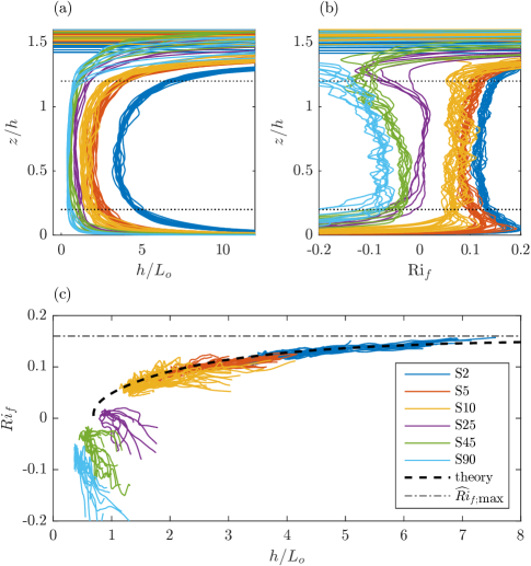
Figure 9: a) Variation with $z/h$ of $h/L_{o}$, as defined in (43); b) Variation with $z/h$ of $\textit{Ri}_{f}$ as defined in (10); c) Variation of $\textit{Ri}_{f}$ with $h/L_{o}$ for various simulations, as denoted in the legend. The theoretical prediction (43) is plotted with a dashed line, and the theoretical maximum value $\textit{Ri}_{f,max}$ is plotted with a dot-dashed line. For the time interval over which results are presented see Table 1 .

It is important to appreciate however that the connection is not complete. In the temporal gravity current flows considered here, we do not observe a transition to intermittency as Ri increases above its critical value, in contrast to the dynamics observed in stratified plane Couette flow by Deusebio2015. Rather the temporal gravity current flows still sustain turbulence, just the entrainment ceases to be significant. This might indicate a difference between flows driven via a body force or via boundary forcing, with temporal gravity currents falling in the former and stratified Couette flow falling in the latter category.

Another important issue to consider is that the observed numerical value of $Ri_{max}\simeq 0.15$ is quite close to $1/4$, the value at the heart of the well-known Miles-Howard criterion for linear normal mode stability of inviscid parallel steady stratified shear flows, and consistent with observations of Ri close to 1/4 in the equatorial undercurrent (Smyth2013). Thorpe2009 conjectured that this is not a coincidence, with the flow being in a state of ‘marginal’ stability. As soon as the mean flow properties are perturbed such that the Richardson number drops below $1/4$, shear instabilities are triggered which, through enhanced dissipation and mixing, push the mean flow properties back towards conditions corresponding to $\textit{Ri}\simeq 1/4$.

Such a ‘kind of equilibrium’ was actually also hypothesised by Turner1973, and is also at least somewhat related to the concept of ‘self-organized criticality’ discussed in §1. At this stage, it is not possible to confirm or disprove the conjecture of the relevance of the Miles-Howard criterion, although within these particular gravity current flows, there are at least two characteristics which challenge this conjecture. First, there is always turbulence present, and so in particular the mean profiles are never actually realised precisely by the flow, calling into question whether it is actually appropriate to consider their linear stability. Second, we do not observe the assumed ‘bursting’ of shear instabilities as the Richardson number drops below some value instantaneously, rather the flow sustains turbulence in a regime where Ri remains sufficiently small, and nontrivially smaller than $1/4$ in point of fact.

It also is interesting to note that Krug2015 reported an equilibrium Richardson number of approximately 0.1 for two spatially developing gravity currents with different initial Richardson number $\textit{Ri}(0)$ and observed a cyclic buildup of velocity and density gradients followed by their destruction by mixing and molecular diffusion. This is somewhat reminiscent of Thorpe’s marginal stability interpretation, even though, as is the case in the present study, the flow never relaminarizes. The cyclic behavior observed in Krug et al. (2015) exhibits local bursts of vigorous turbulence followed by more quiescent periods. For the stronger stratification case, the flow experiences stronger excursions (i.e. higher gradients), but flow states inevitably revolved about the same central equilibrium of buoyancy versus shear.

Nevertheless, despite these caveats, the simulations presented here constitute further evidence that such an approach to a relatively weakly stratified equilibrium for stratified shear flows may well be a generic property of turbulent stratified flows. This has profound implications for the parameterization and interpretation of mixing, and certainly suggests that the classical hypotheses of Ellison1957 concerning the accessibility of large values of the turbulent Prandtl number should be revisited critically.

6 Conclusions

In this paper, we have revisited the classical entrainment experiments of Ellison1959 for gravity currents on inclined slopes, focussing exclusively on the shear-driven entrainment and mixing across the ‘top’ of the gravity current. Using direct numerical simulations that are run for durations long enough for the flow to reach both self-similarity in mean profiles of velocity and buoyancy, and a dynamical equilibrium between the competing effects of buoyancy and shear, we can demonstrate that the net effect of inner layer processes on entrainment and mixing in the outer layer is very small. In all simulations we found that the turbulence is in a local equilibrium in that turbulence production (primarily due to shear) is in equilibrium with dissipation and TKE transport is insignificant. We observed that for the simulations with $\alpha\leq 10^{o}$ the turbulent diffusivity and dissipation rate can be parameterised using the turbulence kinetic energy $e$ and strain rate $S$, which can be used to predict the mixing parameters $\textit{Ri}_{f}$, $\textit{Ri}_{g}$ and $\Gamma$ as a function of $\alpha$.

Both the simulations and the model point to a critical Richardson number $\textit{Ri}_{\textrm{max}}$ as $\alpha\rightarrow 0$, which cannot be exceeded. The model predicts an entrainment law $E=0.31(\textit{Ri}_{\textrm{max}}-\textit{Ri})$, where $\textit{Ri}_{\textrm{max}}\simeq 0.15$ which is in good agreement with our numerical results. This entrainment law hence predicts that $E\rightarrow 0$, i.e. entrainment switches off, for $\textit{Ri}\rightarrow\textit{Ri}_{\textrm{max}}$. One of the main objectives of the paper was to understand better what happens at this critical $\textit{Ri}_{\max}$ when $E\rightarrow 0$. We showed that under these conditions, although the entrainment apparently ‘switches off’, the turbulence itself does not switch off, but rather becomes effectively insignificant. Thus, even though $\Gamma$, $\textit{Ri}_{f}$ and indeed even $\textit{Ri}_{g}$ become maximal as the slope angle $\alpha\rightarrow 0$, the entrainment itself becomes higher order, and effectively negligible. This is because the mean flow parameters, i.e. $S$ and $N$ become larger. This is due to the body force in our particular flow, since as $\alpha$ decreases to very small values the flow continues to accelerate until the shear is sufficiently large to produce a sufficient amount of turbulence. Thus, quantities scaled with mean flow parameters like $e_{T}/u_{T}^{2}\rightarrow 0$, and hence the turbulence becomes ineffective. Ellison’s conjecture was that turbulence could continue to be maintained at large Ri and thus, since $\textit{Ri}_{f}\leq 1$, from (14), the turbulent Prandtl $Pr_{T}$ has to diverge in order to switch off entrainment. We showed that turbulence indeed remains active as $\textit{Ri}\rightarrow\textit{Ri}_{\max}$, but it becomes insignificant and $Pr_{T}\simeq 0.8$ remains finite.

In a fundamental fluid dynamical context, the findings in this paper are consistent with those of previous work which focussed on the small-space aspects associated with the outer interface separating turbulent and non-turbulent regions that controls the mass flux of outer fluid into the turbulent region. This so-called turbulent-nonturbulent interface (TNTI) involves viscous diffusion of vorticity at a rate that is governed by the local energy dissipation rate and kinematic viscosity. The TNTI drives a local entrainment velocity $v_{n}$ that is proportional to the Kolmogorov velocity scale $u_{\eta}$ over its convoluted surface area $A_{\eta}$. We can write the entrainment rate (Krug2013; vanReeuwijk2017) as $E=v_{n}A_{\eta}/(u_{T}A)$, which involves the product of the ratio between the local entrainment velocity and outer velocity scale and the ratio between the surface area of the TNTI and its projected area $A$. Both ratios were shown to decrease with stratification level in Krug2013 and vanReeuwijk2017 hence depleting $E$. The present study suggests that, at critical $Ri$, $v_{n}/u_{T}\rightarrow 0$ because turbulence intensity goes to zero, while we also have that $A_{\eta}/A\rightarrow 1$ because the scaling exponent of the TNTI goes to zero (Krug2017). The latter is caused by the fact that the vertical dimension of the interface scales as $e^{1/2}/S$ for this flow, which tends to zero as $\textit{Ri}\rightarrow\textit{Ri}_{\text{max}}$. Thus, the micro-scale and macro-scale viewpoints are fully consistent, as one would expect them to be.

We conjecture that at least some of the aspects of this flow may be generic among different stratified flows (including for example plane Couette flow). The critical aspect appears to be that the velocity field and buoyancy field adjust so that they reach a balance and direct effects of buoyancy production on turbulence and mixing are relatively small, thus leading to mixing properties consistent with Osborn’s classical mixing parameterisation, and a turbulent Prandtl number $Pr_{T}\sim O(1)$. In particular, there is no evidence of scaled mixing, quantified by such quantities as the flux Richardson number $\textit{Ri}_{f}$ and the turbulent flux coefficient $\Gamma$, exhibiting non-monotonic variation with stratification as commonly observed experimentally (Linden1979). Just as in plane Couette flow (Zhou2017), such flows can only access the weakly stratified ‘left flank’ of such mixing curves. In the nomenclature of Mater2014, these flows are ‘shear-dominated’, and indeed they appear never to be able to be in the ‘buoyancy-dominated’ regime. It is still unclear why the particular value of $\textit{Ri}_{\textrm{max}}\simeq 0.15$ is selected as the critical value, in particular as to whether it has any relationship to the Miles-Howard criterion, and further research is undoubtedly needed to understand why this value arises, and why the mixing dynamics appears to be inevitably located on this inherently ‘shear-dominated’ ‘left flank’.

Furthermore, it is also important to remember that in this paper we have focussed exclusively on one specific entrainment and mixing mechanism associated with gravity currents, the shear-driven mixing at the top of a current, driven by buoyancy when propagating down a slope of finite, yet potentially small, angle. Naturally, in geophysical contexts, other processes are significant, and may indeed be leading order. Such processes include of course, turbulence induced by other mechanisms, for example bottom roughness, tidal motions, and breaking waves. Furthermore, mixing may be dominated by the dynamics in the immediate vicinity of the gravity current’s head, while the current itself may be forced by pressure gradients or indeed other mechanisms not directly related to the along-slope component of the buoyancy force, which slope is often extremely small, and generically not constant. The results presented here could thus be interpreted as demonstrating when the potential significance of such shear-driven entrainment should be considered when assembling a full picture of the entrainment and mixing dynamics of geophysically relevant gravity current flows.