Cool core disturbed: Observational evidence for coexistence of sub-sonic sloshing gas and stripped shock-heated gas around the core of RX J1347.5–1145

Abstract

RX J1347.5–1145 ($z=0.451$) is one of the most luminous X-ray galaxy clusters, which hosts a prominent cool core and exhibits a signature of a major merger. We present the first direct observational evidence for sub-sonic nature of sloshing motion of the cool core. We find that a residual X-ray image from the Chandra X-ray Observatory after removing the global emission shows a clear dipolar pattern characteristic of gas sloshing, whereas we find no significant residual in the Sunyaev-Zel’dovich effect (SZE) image from the Atacama Large Millimeter/submillimeter Array (ALMA). We estimate the equation of state of perturbations in the gas from the X-ray and SZE residual images. The inferred velocity is $420^{+310}_{-420}$ km s^-1, which is much lower than the adiabatic sound speed of the intracluster medium in the core. We thus conclude that the perturbation is nearly isobaric, and gas sloshing motion is consistent with being in pressure equilibrium. Next, we report evidence for gas stripping of an infalling subcluster, which likely shock-heats gas to high temperature well in excess of 20 keV. Using mass distribution inferred from strong lensing images of the Hubble Space Telescope (HST), we find that the mass peak is located away from the peak position of stripped gas with statistical significance of $>5\sigma$. Unlike for the gas sloshing, the velocity inferred from the equation of state of the excess hot gas is comparable to the adiabatic sound speed expected for the 20 keV intracluster medium. All of the results support that the southeast substructure is created by a merger. On the other hand, the positional offset between the mass and the gas limits the self-interaction cross section of dark matter to be less than $3.7~{}h^{-1}~{}{\rm cm^{2}~{}g^{-1}}$ (95% CL).

1 Introduction

Galaxy clusters are the largest gravitationally-bound and virialized objects in the universe. They are located at the knots of filaments in the large-scale structure and provide us with unique cosmological information. Galaxy clusters are also dynamically young and are continuously growing through mergers between smaller clusters. Such merger activities induce various high-energy phenomena in the hot and optically thin plasma, i.e., the intracluster medium (ICM), in the gravitational potential well of clusters.

A large amount of observational and numerical studies have suggested that mergers lead to shock-heating of the gas (e.g., Ricker & Sarazin, 2001; Markevitch et al., 2002; Takizawa, 2005, 2006; Bourdin et al., 2013), production of cold fronts (e.g., Markevitch et al., 2001; Ascasibar & Markevitch, 2006; ZuHone et al., 2010; Roediger et al., 2011; Blanton et al., 2011; Ueda et al., 2017; Hitomi Collaboration et al., 2018), ram-pressure stripping of the gas from infalling galaxies (e.g., David & Kempner, 2004; Roediger & Brüggen, 2007; Sasaki et al., 2016), non-equilibrium ionization of the ICM (e.g., Akahori & Yoshikawa, 2008, 2010, 2012; Inoue et al., 2016), and (re-) acceleration of relativistic particles (e.g., Feretti et al., 2012; Akamatsu & Kawahara, 2013; Brunetti & Jones, 2014; van Weeren et al., 2017). The entire picture of merging processes is however still far from clear; for example, heating mechanisms and dynamics of the ICM are under debate. Observational studies in multi-wavelength are therefore crucial for understanding the physics of galaxy cluster mergers.

RX J1347.5–1145 is one of the most luminous X-ray galaxy clusters and is located at the redshift of $z=0.451$. It was thought to be a relaxed cluster when it was discovered in the ROSAT all sky survey (Schindler et al., 1997). Komatsu et al. (1999) made the first measurements of the Sunyaev-Zel’dovich effect (SZE: Sunyaev & Zeldovich, 1972) toward this cluster with the James Clerk Maxwell Telescope (JCMT) at 350 GHz as well as with the 45 m Nobeyama Radio Telescope at 21 and 43 GHz. A higher angular resolution observation of the SZE was performed by Komatsu et al. (2001) using the Nobeyama Bolometer Array (NOBA) and they found a prominent substructure which has no counterpart in the soft X-ray image by ROSAT. The presence of the substructure has been confirmed by Chandra and XMM-Newton (e.g., Allen et al., 2002; Gitti & Schindler, 2004) as well as by more recent SZE measurements (Mason et al., 2010; Korngut et al., 2011; Plagge et al., 2013; Adam et al., 2014; Kitayama et al., 2016). Allen et al. (2002) measured the mean temperature of the ICM to be over 10 keV, which is relatively high compared to other typical clusters. Kitayama et al. (2004) and Ota et al. (2008) found a very hot ($>20$ keV) component of the ICM in this cluster. In addition, the radial profile and spatial distribution of the ICM temperature indicate that the temperature drops to $\sim 6$ keV toward the cluster center so that the cool core is formed (e.g., Allen et al., 2002; Ota et al., 2008; Kreisch et al., 2016). A disturbed morphology is furthermore supported by the radio synchrotron observations (e.g., Ferrari et al., 2011) and the gravitational lensing maps (e.g., Köhlinger & Schmidt, 2014). The total mass of RX J1347.5–1145 within $r_{200}$ is estimated to be $\sim 1.5\times 10^{15}\,h^{-1}$ $M_{\odot}$ by using the weak-lensing analysis, where $r_{200}$, the radius within which the mean mass density is 200 times the critical density of the universe, is $1.85\,h^{-1}$ Mpc (Lu et al., 2010) for this galaxy cluster.

It is considered that the hot component is most likely associated with a past major merger event (e.g., Johnson et al., 2012; Kreisch et al., 2016), although its specific nature, such as geometry and dynamics of the collision, is still unclear. Recently, Kitayama et al. (2016) presented the SZE image observed by Atacama Large Millimeter/submillimeter Array (ALMA) with angular resolution of 5″. Such high angular resolution enables us to remove the emission of the central active galactic nucleus (AGN) and to reconstruct an accurate SZE map. Kitayama et al. (2016) found that the shape of the SZE is elongated toward the southeast and the peak position of the SZE is located at 11″ southeast from the central AGN. The ALMA high-resolution SZE image motivates us to directly compare it with high-quality data in other wavelengths by Chandra and Hubble Space Telescope (HST). In this paper, we investigate the merger phenomena and merger history in RX J1347.5–1145 by combining the data of Chandra, ALMA, and HST.

We adopt $\Omega_{\rm m}=0.3$ and $\Omega_{\rm\Lambda}=0.7$. We use the dimensionless Hubble constant ($h\equiv H_{0}/100\,$km s^-1 Mpc^-1); given controversial results on the value of $h$ (e.g., Planck Collaboration et al., 2016; Riess et al., 2016), we do not fix it unless stated otherwise. In this cosmology, an angular size of $1^{\prime\prime}$ corresponds to a physical scale of 4.04 $h^{-1}$ kpc at the redshift $z=0.451$. Unless stated otherwise, quoted errors correspond to 1$\sigma$.

2 Observations and Data Reductions

We used the X-ray data of RX J1347.5–1145 taken with the Advanced CCD Imaging Spectrometer (ACIS; Garmire et al., 2003) on board Chandra. Two out of six datasets we used were taken by ACIS-S (ObsID: 506 and 507) and the others were by ACIS-I (ObsID: 3592, 13516, 13999, and 14407). All the datasets are the same as used in our previous study (Kitayama et al., 2016). The data reduction is also the same as in Kitayama et al. (2016), except that we used the updated versions, 4.9 and 4.7.5.1, of Chandra Interactive Analysis of Observations (CIAO; Fruscione et al., 2006) and the calibration database (CALDB), respectively. The background data were extracted from the region between $2.5^{\prime}$ and $3.5^{\prime}$ from the peak position of the cluster. Unless stated otherwise, we used XSPEC version 12.9.1$l$ (Arnaud, 1996) and the atomic database for plasma emission modeling (AtomDB) version 3.0.9 in the X-ray spectral analysis, assuming that the ICM is in a collisional ionization equilibrium. The Galactic absorption was fixed at $N_{\rm H}=4.6\times 10^{20}$ cm^-2 (Kalberla et al., 2005). We adopted the abundance table of Anders & Grevesse (1989) in the X-ray spectral analysis.

The ALMA SZE data used in this paper are the same as those in Kitayama et al. (2016), except that an updated version, 5.1.1, of the Common Astronomy Software Applications (CASA: McMullin et al., 2007) was adopted in the imaging analysis.

We also used the data of HST observations of RX J1347.5–1145 obtained with the Advanced Camera for Surveys (ACS) to study the central mass distribution from strong lensing (SL). These data were provided by the Space Telescope Science Institute (STScI) and no additional data reduction was applied in this study. The data consisted of F475W, F814W, and F850LP images from the ACS, which were used in Halkola et al. (2008), Köhlinger & Schmidt (2014), and Zitrin et al. (2015).

3 X-ray and SZE Analyses

3.1 X-ray and SZE imaging analysis

Figure 1 shows the X-ray surface brightness (left) and the SZE image (right) of RX J1347.5–1145, respectively, both of which clearly exhibits a substructure in the southeast direction. First, we computed the mean X-ray surface brightness over an ellipse, excluding the southeast quadrant (i.e., the substructure), following Ueda et al. (2017). To accurately model the mean surface brightness profile, we searched for the ellipse that minimizes the variance of the X-ray surface brightness relative to its mean in a $15^{\prime\prime}<\bar{r}<35^{\prime\prime}$ annulus, where $\bar{r}$ is the geometrical mean of the semi-major and semi-minor axis lengths around the X-ray peak. The range of $\bar{r}$ was chosen to match the position of the excess emission in the excluded southeast quadrant and to eliminate the impact of the bright core ($\bar{r}<10^{\prime\prime}$) of this cluster on the overall shape. We find that the axis ratio of the ellipse is 0.66 and its position angle is $-8.7^{\circ}$ . The resultant annulus is shown in the left panel of Figure 1. We then calculated the mean X-ray brightness over the ellipse at each $\bar{r}$, excluding the southeast quadrant, and subtracted it from the entire brightness. The left panel of Figure 2 shows an X-ray residual image of RX J1347.5–1145.

We also applied the same procedure for the SZE image. The obtained SZE residual image is shown in the right panel of Figure 2. Note that we used the unsmoothed SZE image with the synthesized beam size of $4.1^{\prime\prime}\times 2.5^{\prime\prime}$ FWHM (Kitayama et al., 2016) in the SZE imaging analysis. The smoothed images are shown only for display purposes.

Figure 2 clearly shows an excess signal in the southeast quadrant both in the X-ray and SZE images. Thanks to the high-resolution data, we find that the excess SZE signal has the average FWHM of $\sim 28^{\prime\prime}$ (113 $h^{-1}$ kpc), which is significantly more extended than that of $\sim 17^{\prime\prime}$ (69 $h^{-1}$ kpc) in the X-ray residual image. This indicates that a high temperature region has a larger extent than seen in X-rays. We will present more detailed analyses and results on this region using two independent methods in Section 3.2 and Section 3.3.

A dipolar pattern around the central AGN is apparent only in the X-ray residual image (the left panel of Figure 2). The dipolar pattern consists of a northern positive excess and a southern negative excess. The fraction of each component against the mean brightness is roughly 20 %. The dipolar pattern is clearly distinct from the excess in the southeast quadrant and extends over a spatial scale of $\sim 100$ $h^{-1}$ kpc. We will describe more detailed results in Section 3.4.

We assessed the uncertainty in subtracting the mean profile of the X-ray and SZE images by the following two methods. One is the same method as described above, except that the subtraction of the mean profile is done after smoothing the X-ray image to the same angular resolution as the ALMA image. The other is that we assumed circular symmetry for the mean profile of X-rays and SZE instead of the ellipse. In this check, we do not use any smoothed images. We then find that 1) a difference of angular resolution between Chandra and ALMA does not affect the residual images, and 2) the geometry of the mean profile does not affect the substructure in the southeast quadrant, while it slightly modifies the shape of the dipolar pattern in the core.

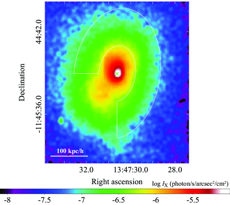
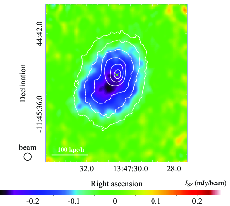
Figure 1: Surface brightnesses of the X-ray (left) and the SZE (right) of RX J1347.5–1145. The green cross corresponds to the position of the central AGN identified by ALMA at 92 GHz. Left: The X-ray surface brightness in the $0.4-7.0$ keV band is shown as the logarithm value in units of photon sec^-1 arcsec^-2 cm^-2. This image is smoothed by the Gaussian kernel with $2.3^{\prime\prime}$ FWHM. Overlaid is a white elliptical annulus within which variation of this surface brightness is minimized at the mean radius between $15^{\prime\prime}$ and $35^{\prime\prime}$, excluding the southeast quadrant. Right: The SZE surface brightness overlaid with the contours of the X-ray surface brightness, corresponding to 64, 32, 18, 8, 4, and 2 $\%$ of the peak value, after being smoothed by the Gaussian kernel with $2.3^{\prime\prime}$ FWHM. Colors indicate the ALMA SZE map in mJy beam^-1 smoothed to a beam size of $5^{\prime\prime}$ FWHM. The beam size is presented as a black circle out of the map.

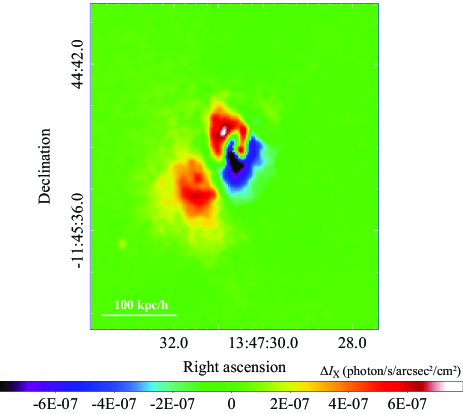
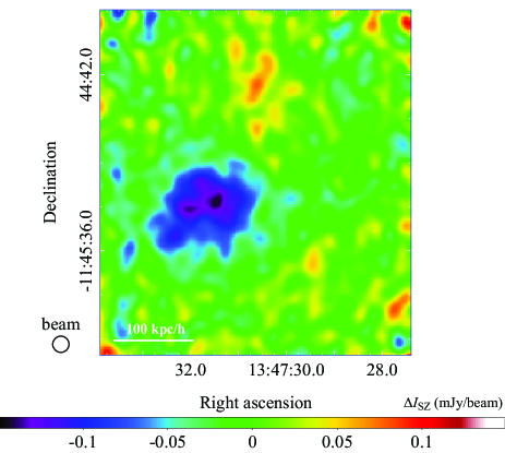
Figure 2: Residual images of the X-ray and SZE surface brightness. Left: The residual image of Chandra X-ray surface brightness after subtracting the mean profile, excluding the southeast quadrant. The original surface brightness is the same as the left panel of Figure 1. For reference, the position of the central AGN is marked by a cross. Right: Same as the left panel but for the ALMA 92 GHz brightness in mJy beam^-1 with the effective beam size of $5^{\prime\prime}$ FWHM. The original surface brightness is shown in the right panel of Figure 1.

3.2 X-ray spectral analyses of the southeast substructure

To understand the origin and thermodynamic properties of the ICM in the southeast substructure, we performed X-ray spectral analyses. We defined nine regions covering the excess and its surrounding along the ellipse as in Section 3.1 (i.e., Region 1a, 1b, 1c, 2a, $\cdots$, 3b, and 3c) and three regions covering the remaining parts of the ellipse (i.e., Region 1d, 2d, and 3d) as illustrated in Figure 3. First, we assumed, for simplicity, that the ICM in each region consists only of a single component over the entire line-of-sight. Its temperature ($kT_{\rm single}$) was measured using a model phabs * apec in XSPEC, where phabs represents the Galactic absorption (Balucinska-Church & McCammon, 1992). The photon counts in $0.4-7.0$ keV and the best-fit parameters are summarized in Table 1.

Second, we adopted a two-component model in which an excess component is embedded in an ambient component in the nine regions. The ambient component was assumed to have the same temperature as the gas temperature in an annulus at the same $\bar{r}$ (i.e., $kT_{\rm single}$ of Region 1d, 2d, and 3d). We then measured the temperature of the excess component ($kT_{\rm excess}$) by using the two apec model, fixing the temperature of the ambient component at the best-fit value of $kT_{\rm single}$ in Region 1d, 2d, and 3d, respectively. The spectral normalization of the ambient component was scaled by each interested sky area. The best-fit parameters of the excess component are shown in Table 1. We also estimated the electron density of the excess component ($n_{\rm excess}$) assuming that it is uniform over a line-of-sight extent of $L_{\rm excess}=150$ kpc, which is similar to the projected size of the substructure on the sky. For different values of $L_{\rm excess}$, the electron density scales as $L_{\rm excess}^{-1/2}$. In addition, we calculated the thermal pressure of the excess electrons ($p_{\rm excess}$), i.e., $n_{\rm excess}\times kT_{\rm excess}$. In above analyses, we fixed the metal abundance of the ICM at 0.38 solar based on previous X-ray measurements (Ota et al., 2008).

Figures 4, 5, and 6 show the spatial maps of $kT_{\rm excess},n_{\rm excess}$, and $p_{\rm excess}$ (left panels are their best-fits and right panels are corresponding statistical error), respectively. We find that the electron density of excess component in Region 1b is the highest among the nine regions, which agrees with the peak position in the X-ray residual image. On the other hand, while the statistical error is large, the temperature of the excess component in Region 2b is estimated to be $\sim 30$ keV, which is the highest among the nine regions. The highest temperature region is located at $\sim 27^{\prime\prime}$ away from the center, which is well outside the cool core. Note that the X-ray emission in Region 2b is faint but the SZE signal is prominent. This means that the ALMA SZE data play a crucial role in identifying such excess hot gas. The thermal pressure of the excess electrons ($p_{\rm excess}$) is nearly constant among Regions 1b, 2b, and 1c, as presented in Table 1. This is in good agreement with the excess SZE signal shown in the right panel of Figure 3. The thermal energy of the excess electrons in Region 1b, 2b, and 1c is estimated to be $\sim 1.1\times 10^{61}\,h^{-2}$ erg, $\sim 1.6\times 10^{61}\,h^{-2}$ erg, and $\sim 2.0\times 10^{61}\,h^{-2}$ erg, respectively.

We estimated the Mach number $\cal M$ from the Rankine-Hugoniot jump condition, assuming the ratio of specific heats as $\gamma=5/3$,

$$\frac{T_{2}}{T_{1}}=\frac{5{\cal M}^{4}+14{\cal M}^{2}-3}{16{\cal M}^{2}},$$ (1)

where $T_{1}$ is the pre-shock temperature and $T_{2}$ is the post-shock temperature. Using the observed temperature jump between Region 2a and 2b and propagating the statistical errors, we obtain ${\cal M}=1.68^{+0.69}_{-0.47}$. The adiabatic sound speed of the gas in Region 2a is estimated to be $2140^{+300}_{-180}$ km s^-1, implying a shock speed of the gas in Region 2b as $3590^{+1560}_{-1050}$ km s^-1.

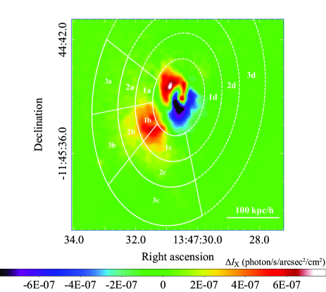
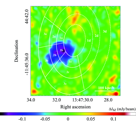
Figure 3: Same as Figure 2, except that elliptical annuli used in the X-ray spectral analysis are overlaid.

Table 1: Best-fit parameters to the X-ray spectra in each region shown in Figure 3. The metal abundance is fixed at each of 0.38 $Z_{\odot}$. The photon counts are background-subtracted. $kT_{\rm single}$ is obtained by a single component model in the 12 regions. $kT_{\rm excess}$ and $n_{\rm excess}$ are obtained by a two-component fit in each region, fixing the temperature of the ambient component at the best-fit values for the same annulus region (i.e., $kT_{\rm single}$ of Region 1d, 2d, and 3d). We show the statistical errors alone.

Region	1a	1b	1c	1d
Photon counts in $0.4-7.0$ keV	4566	8023	10917	21083
$kT_{\rm single}$ (keV)	$18.5^{+2.2}_{-2.1}$	$18.2^{+1.9}_{-1.6}$	$19.5^{+1.6}_{-1.6}$	$15.7^{+0.7}_{-0.7}$
$kT_{\rm excess}$ (keV)	$21.8^{+8.6}_{-4.9}$	$20.3^{+4.7}_{-3.1}$	$24.2^{+6.1}_{-3.8}$	–
$n_{\rm excess}$ ($10^{-2}$ cm-3 $(L_{\rm excess}/150\,{\rm kpc})^{-1/2}$)	$2.53^{+0.06}_{-0.04}$	$3.71^{+0.04}_{-0.04}$	$2.97^{+0.04}_{-0.04}$	–
$p_{\rm excess}$ (keV cm-3 $(L_{\rm excess}/150\,{\rm kpc})^{-1/2}$)	$0.552^{+0.218}_{-0.124}$	$0.753^{+0.175}_{-0.115}$	$0.719^{+0.181}_{-0.113}$	–
Region	2a	2b	2c	2d
Photon counts in $0.4-7.0$ keV	3208	4824	5996	12623
$kT_{\rm single}$ (keV)	$17.8^{+3.1}_{-1.8}$	$24.6^{+4.3}_{-3.6}$	$14.8^{+1.5}_{-1.5}$	$19.5^{+1.6}_{-1.6}$
$kT_{\rm excess}$ (keV)	$17.2^{+4.8}_{-2.9}$	$29.1^{+9.4}_{-6.9}$	$11.7^{+2.0}_{-1.5}$	–
$n_{\rm excess}$ ($10^{-2}$ cm-3 $(L_{\rm excess}/150\,{\rm kpc})^{-1/2}$)	$1.93^{+0.06}_{-0.05}$	$2.55^{+0.06}_{-0.06}$	$1.77^{+0.03}_{-0.03}$	–
$p_{\rm excess}$ (keV cm-3 $(L_{\rm excess}/150\,{\rm kpc})^{-1/2}$)	$0.332^{+0.093}_{-0.057}$	$0.742^{+0.240}_{-0.177}$	$0.207^{+0.036}_{-0.027}$	–
Region	3a	3b	3c	3d
Photon counts in $0.4-7.0$ keV	3337	3682	4281	9987
$kT_{\rm single}$ (keV)	$17.9^{+3.1}_{-2.5}$	$21.3^{+4.0}_{-3.1}$	$17.2^{+2.2}_{-1.1}$	$20.2^{+1.9}_{-1.7}$
$kT_{\rm excess}$ (keV)	$16.5^{+4.9}_{-3.2}$	$22.1^{+8.9}_{-5.2}$	$14.9^{+4.8}_{-3.6}$	–
$n_{\rm excess}$ ($10^{-2}$ cm-3 $(L_{\rm excess}/150\,{\rm kpc})^{-1/2}$)	$1.40^{+0.04}_{-0.04}$	$1.34^{+0.05}_{-0.04}$	$0.88^{+0.03}_{-0.02}$	–
$p_{\rm excess}$ (keV cm-3 $(L_{\rm excess}/150\,{\rm kpc})^{-1/2}$)	$0.231^{+0.069}_{-0.045}$	$0.296^{+0.120}_{-0.070}$	$0.131^{+0.042}_{-0.032}$	–

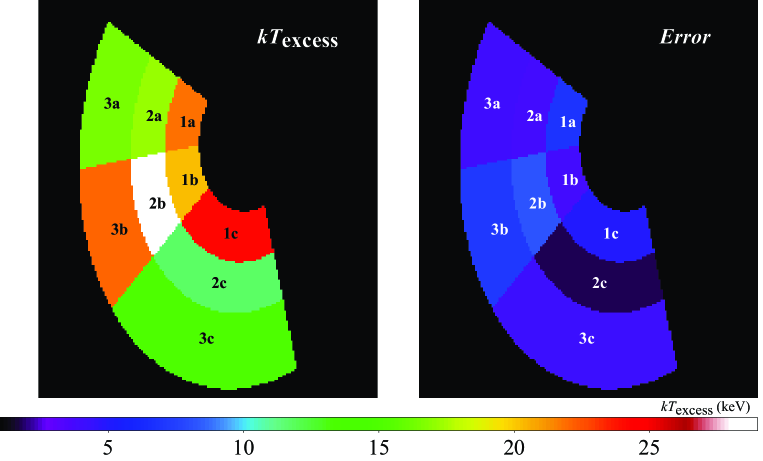
Figure 4: Temperature (left) and average of its statistical error (right) maps of the excess component ($kT_{\rm excess}$) in nine regions in units of keV. All the best-fit values are the same as shown in Table 1, while the error values are the average of upper and lower statistical errors of each region.

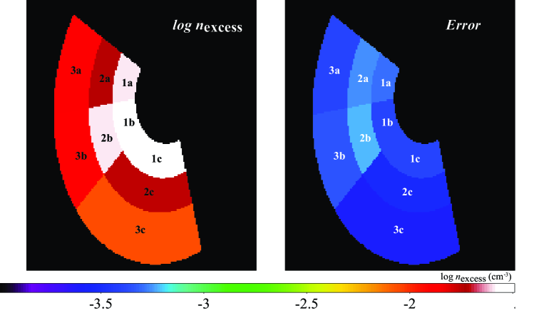
Figure 5: Same as Figure 4 but for the logarithm of electron density of the excess component ($\log n_{\rm excess}$) in units of $\log$ cm^-3. The values are approximately proportional to $(L_{\rm excess}/150\,{\rm kpc})^{-1/2}$.

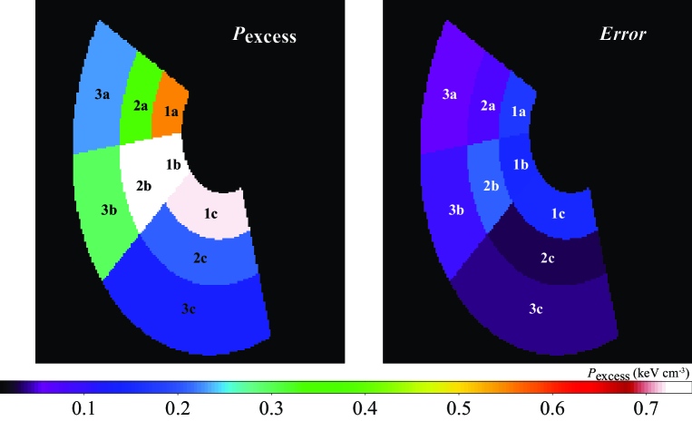
Figure 6: Same as Figure 4 but for the thermal pressure of the excess electrons ($p_{\rm excess}$) in units of keV cm^-3. The values are also approximately proportional to $(L_{\rm excess}/150\,{\rm kpc})^{-1/2}$.

3.3 Combined analysis of SZE and X-ray imaging data for the excess component

As an alternative measure of the gas temperature and electron density, we combined the SZE and X-ray images. We used SPEX version 3.04.00 for the X-ray data analysis and CASA version 5.1.1 for the SZE data analysis. Note that the analysis in this section does not rely on X-ray spectra and is fully independent of that presented in Section 3.2.

We measured the intensities of X-ray ($\Delta I_{\rm X}$) and SZE ($\Delta I_{\rm SZ}$) of the X-ray and SZE residual images shown in Figure 2. Both images were binned so that the angular resolutions of Chandra and ALMA have a common pixel size of $5^{\prime\prime}\times 5^{\prime\prime}$. The two intensities are then described as

$$\Delta I_{\rm X} \propto n_{\rm excess}^{2}\times\Lambda(T_{\rm excess})\times L_{\rm excess},$$ (2)

$$\Delta I_{\rm SZ} \propto n_{\rm excess}\times kT_{\rm excess}\times L_{\rm excess}\times f_{r}(T_{\rm excess})\times f_{c},$$ (3)

respectively, where $\Lambda$ is the X-ray emissivity over the energy range $0.4-7.0$ keV, $f_{r}$ is the relativistic correction to the SZE intensity (Itoh & Nozawa, 2004), and $f_{c}$ is a correction factor for the missing flux in the ALMA data. We set $f_{c}$ to be equal to the parameter $c_{1}=0.88$ in Equation (2) of Kitayama et al. (2016) derived from detailed imaging simulations for RX J1347.5–1145. We then solved Equations (2) and (3) for $n_{\rm excess}$ and $kT_{\rm excess}$, respectively, assuming $L_{\rm excess}=150$ kpc as in Section 3.2. For different values of $L_{\rm excess}$, they approximately scale as $kT_{\rm excess}\propto L_{\rm excess}^{-1/2}$ and $n_{\rm excess}\propto L_{\rm excess}^{-1/2}$, if weak dependences of $\Lambda$ and $f_{r}$ on temperature is neglected. We focused on the high significance pixels for which the signal-to-noise ratios (S/N) of $\Delta I_{\rm X}$ and $\Delta I_{\rm SZ}$ are both over $4\sigma$. Figure 7 shows the measured temperature of the excess component (left) and its statistical error (right). Figure 8 is the same as Figure 7 but for the electron density of the excess component. The typical errors of temperature and electron density are about 4 keV and $0.05\times 10^{-2}$ cm^-3, respectively.

We find that the highest temperature region is located in Region 2b. This result is consistent with that measured with an independent method using the X-ray spectra (Section 3.2). We also find that the highest electron density region is in Region 1b. In addition, we estimate the thermal energy of the excess electrons to be $(1.9\pm 0.1\,({\rm stat.})\pm 0.7\,({\rm sys.}))\times 10^{61}$ $h^{-2}$ erg from the SZE residual image directly, within a radius of 50 $h^{-1}$ kpc around the peak of the SZE residual signal. Further details of the systematic uncertainty are mentioned in Section 3.5. The angular resolution and sensitivity of the previous SZE observations did not match those of the X-ray data. The ALMA SZE data allow us, for the first time, the detailed comparison with the X-ray data with comparable resolution and sensitivity.

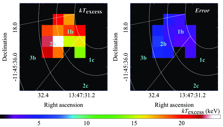
Figure 7: Temperature of the excess component in units of keV (left) and its statistical error (right) inferred from the ALMA SZE and Chandra X-ray images, assuming a constant line-of-sight length of $L_{\rm excess}=150$ kpc. The values are approximately proportional to $(L_{\rm excess}/150\,{\rm kpc})^{-1/2}$. Regions for which S/N of either data are less than $4\sigma$ are left blank (black colored). For reference, the elliptical annuli shown in Figure 3 are overlaid. Note that X-ray spectra are not used in computing the quantities plotted in this figure.

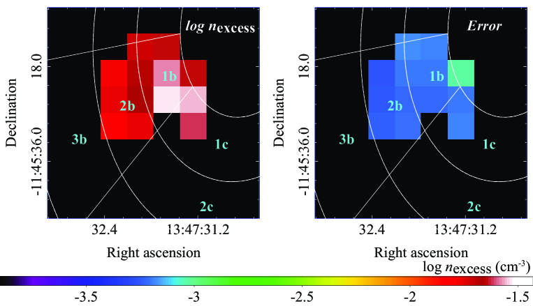
Figure 8: Same as Figure 7, but for the logarithm of electron density (left) and its statistical error (right) in units of cm^-3. The values are also approximately proportional to $(L_{\rm excess}/150\,{\rm kpc})^{-1/2}$.

3.4 Nature of gas sloshing in the core

The spatial scale of the dipolar pattern is estimated to be $40\,h^{-1}$ kpc by applying the definition of the size described in Ueda et al. (2017). We analyzed the X-ray spectra of the ICM in the region of the dipolar pattern to examine its thermodynamic property. The temperature toward the positive and the negative excess is estimated as $8.8^{+0.2}_{-0.2}$ keV and $10.6^{+0.4}_{-0.3}$ keV, respectively. The metal abundances are $0.47^{+0.03}_{-0.03}$ $Z_{\odot}$ for the positive excess and $0.37^{+0.05}_{-0.05}$ $Z_{\odot}$ for the negative excess. These properties are as expected for gas sloshing, i.e., metal rich, cool, and dense gas is moving around the central galaxy. On the other hand, we find the absence of excess SZE signal in the core, which provides the first direct evidence that the disturbed gas is nearly in pressure equilibrium. This indicates that the gas sloshing motion is sub-sonic.

Here, we shall introduce the “equation of state” of the perturbation in gas, $w\equiv\Delta p/\Delta\rho$. For similar analyses, see Churazov et al. (2016), Khatri & Gaspari (2016), and references therein. If the perturbation is adiabatic, then $w$ is equal to the sound speed squared, i.e., $w=c_{s}^{2}$. If the perturbation is isobaric, we should find $w\ll c_{s}^{2}$. The SZE residual image gives an estimate of the pressure perturbation $\Delta p$, whereas the X-ray residual image gives an estimate of the density perturbation $\Delta\rho$ as

$$\frac{|\Delta I_{\rm X}|}{\langle I_{\rm X}\rangle}\simeq\frac{\Delta\langle n^{2}\rangle}{\langle n^{2}\rangle}\simeq\frac{2\Delta\rho}{\sqrt{\langle\rho^{2}\rangle}}$$ (4)

because $|\Delta I_{\rm X}|\ll\langle I_{\rm X}\rangle$, where $\langle I_{\rm X}\rangle$ is the mean X-ray surface brightness, $\langle n^{2}\rangle$ is the mean square electron number density, and $\langle\rho^{2}\rangle$ is the mean square gas mass density. First, to cover the dipolar pattern in the X-ray residual image, we used the ellipse with the same geometry as mentioned in Section 3.1, with a semi-major axis length of $22^{\prime\prime}$, excluding the southeast quadrant. We extracted the X-ray spectrum for this elliptical sector and carried out the X-ray spectral analysis. Assuming the line-of-sight depth of 100 kpc, the mean ICM temperature and the mean electron number density, $\sqrt{\langle n^{2}\rangle}$, in this region are $9.8\pm 0.2$ keV and $(8.24\pm 0.02)\times 10^{-2}$ cm^-3, respectively. Next, using the X-ray and SZE residual images and assuming the line-of-sight depth of 100 kpc, we measured $\Delta\rho$, $\Delta p$, and their statistical errors within the same elliptical sector. We then find that the velocity inferred from the equation of state is $\sqrt{w}=420^{+310}_{-420}$ km s^-1. This inferred velocity is much lower than the adiabatic sound speed of the 10 keV ICM, $\sim 1630$ km s^-1. The motion of gas sloshing is therefore consistent with being sub-sonic and isobaric.

3.5 Systematic uncertainty of the ICM properties

The systematic uncertainty of the ICM temperature measured with the ACIS is estimated to be $\sim 20$ % for galaxy clusters with high temperature (over 10 keV) ICM like RX J1347.5–1145 (e.g., Reese et al., 2010; Nevalainen et al., 2010; Schellenberger et al., 2015). Note that the statistical uncertainty of the temperature of the excess component is $20\sim 30$ % in the nine regions. We evaluated the impact of the systematic uncertainty on the X-ray and the SZE data for the combined analysis. We applied the 4 % uncertainty of the ACIS effective area , the 6 % uncertainty of the ALMA flux calibration (see Section 2 of Kitayama et al., 2016), and 1.3 $\mu$Jy arcsec^-2 for the ALMA missing flux correction (see Section 4.2 of Kitayama et al., 2016) to the data. The error of the ICM temperature and density including the systematic uncertainty is about twice larger than that shown in the right panels of Figure 7 and 8; for example, the error for the highest temperature region (23.2 keV) changes from $\pm 3.9$ keV to $\pm 8.1$ keV. Note that these systematic uncertainties are only relevant to the absolute values of derived parameters but not their relative trends, in which we are mainly interested.

4 HST strong-lensing analysis

4.1 Central mass distribution

To reveal the geometry of mergers in RX J1347.5–1145, we analyzed the central mass distribution derived by SL. We used the GLAFIC software package (Oguri, 2010) for our mass modeling. GLAFIC adopts a parametrized mass model and derives the best-fit mass map that reproduces the observed positions of SL multiple images. The software has been used for SL mass modeling of many massive clusters (e.g., Oguri et al., 2012; Kawamata et al., 2016) and has also been shown to recover central mass distributions of simulated clusters remarkably well (Meneghetti et al., 2017).

We followed the standard procedure to model massive clusters in which we adopted a few dark halo components, cluster member galaxies, and the external perturbations on the lens potential (see e.g., Kawamata et al., 2016). For dark halo components, we assumed an elliptical extension of the Navarro-Frenk-White (NFW) model (Navarro et al., 1997). Each dark halo component is characterized by a set of parameters including the virial mass, the concentration parameter, positions, the eccentricity of ellipse, and its position angle as model parameters. For member galaxies, we used the scaling relations to reduce the number of model parameters. We constructed a cluster member galaxy catalog by selecting galaxies near the red-sequence in the HST F475W-F814W color-magnitude diagram, where the magnitudes are MAG_APER of SExtractor (Bertin & Arnouts, 1996) with $1^{\prime\prime}$ diameter aperture. The mass distribution of the member galaxies was assumed to follow pseudo-Jaffe ellipsoids whose velocity dispersions and truncation radii scale with galaxy luminosity $L_{\rm gal}$ as $\sigma\propto L_{\rm gal}^{1/4}$ and $r_{\rm trunc}\propto L_{\rm gal}^{1/2}$, respectively. The normalizations of these two scaling relations were treated as model parameters. In addition, to improve the fit, we included external perturbations described by a multipole Taylor expansion of the form $\phi\propto r^{2}\cos m(\theta-\theta_{*})$. We included terms with $m=2$ (external shear), $3$, and $4$. Each term is specified by its amplitude and position angle as model parameters.

For observational constraints, we used the positions of 21 multiple images from six multiple image sets of the lensed galaxies. These multiple images are identified in previous work on this cluster (Halkola et al., 2008; Köhlinger & Schmidt, 2014; Zitrin et al., 2015). In this paper, we reexamined the validity of the previous multiple image identifications in the course of our own mass modeling, and adopted only secure multiple images for our analysis. The redshift of one multiple image set was fixed as the spectroscopic value, whereas for those of four multiple image sets, we included Gaussian priors based on their photometric redshifts. We assumed a positional error of $0\farcs 5$ for all the multiple images, which is a standard value in SL mass modeling (e.g., Kawamata et al., 2016). Table 2 summarizes the data of multiple images for our SL analyses.

Table 2: Data of 21 multiple images from six multiple image sets of the lensed galaxies used for our SL analyses.

ID	R.A. (deg)	Dec. (deg)	$z_{\rm obs}$	Reference
1.1	206.887550	-11.757544	$2.2\pm 0.3$	1
1.2	206.878783	-11.753378
1.3	206.877675	-11.759375
1.4	206.885183	-11.748411
1.5	206.869604	-11.747325
2.1	206.882608	-11.764414	$1.75$	1, 2
2.2	206.871675	-11.760722
2.3	206.872312	-11.761255
3.1	206.874179	-11.745133	$4.1\pm 0.3$	1, 2
3.2	206.872500	-11.746467
3.3	206.871162	-11.748361
3.4	206.872271	-11.757350
3.5	206.891250	-11.760539
3.6	206.876079	-11.744372
4.1	206.884138	-11.741794	$3.6\pm 0.3$	1
4.2	206.882975	-11.741230
4.3	206.892412	-11.751589
5.1	206.878429	-11.749203	NA	1
5.2	206.878317	-11.749703
6.1	206.882320	-11.742199	$6.6\pm 0.3$	3
6.2	206.875980	-11.741229

Our fiducial model contains two dark halo components, which are supposed to model mass distributions near the brightest cluster galaxy (BCG) of the main cluster and the second BCG (hereafter 2nd BCG) that is considered to be the BCG of the subcluster, respectively. This model contains 37 model parameters, which are constrained by 46 observational data points. We also considered another model which contains three dark halo components, as such model may reveal a mass component which does not correspond to either the BCG or the 2nd BCG. In this model, the number of model parameters increases to 43. We evaluated statistical errors of model parameters, such as masses of dark halo, concentration parameters, and mass peaks with Markov chain Monte Carlo (MCMC) methods.

The surface mass density map obtained from the two dark halo components is shown in the left panel of Figure 9. The best-fit parameters are summarized in Table 3. The locations of the two mass peaks are treated as free parameters, while we find that the two mass peaks are in good agreement with the positions of the BCG and the 2nd BCG. The estimated virial masses are $7.2^{+2.1}_{-1.9}\times 10^{14}$ $h^{-1}$$M_{\odot}$ for the main cluster and $2.8^{+2.4}_{-1.1}\times 10^{14}$ $h^{-1}$$M_{\odot}$ for the subcluster. Their concentration parameters are estimated to be $c=6.6^{+1.0}_{-0.9}$ and $c=4.8^{+2.2}_{-1.6}$, respectively. The obtained mass and concentration parameter are correlated strongly, therefore the systematic uncertainty of the mass estimates might be large. Nevertheless their mass ratio indicates that RX J1347.5–1145 is a major merging cluster. The total mass of the subcluster has been previously estimated using the excess X-ray flux and applying the luminosity - mass relation to be $(3.4\pm 1.7)\times 10^{14}$ $h^{-1}$ $M_{\odot}$ (Johnson et al., 2012) and $\sim 2.3\times 10^{14}$ $h^{-1}$ $M_{\odot}$ (Kreisch et al., 2016), which are consistent with that by our SL analysis. The entire mass distribution of RX J1347.5–1145 is slightly elongated along the northeast direction.

The right panel of Figure 9 shows the surface mass density map obtained from the three dark halo components. The mass of the third component is weakly constrained to be $1.4\times 10^{14}$ $h^{-1}$ $M_{\odot}$ (95% CL). The location of the third component is also poorly determined, but it lies to the northeast of the BCG. These indicate that the mass distribution of dark matter (DM) near the center and in the southeast quadrant of RX J1347.5–1145 is well modeled by the two dark halo components. We therefore neglect the third dark halo component in the rest of this paper.

Table 3: Best-fit parameters of mass distributions of the main cluster and the subcluster measured by SL

	Main cluster	Subcluster
Mass ($10^{14}\,h^{-1}$$M_{\odot}$)	$7.2^{+2.1}_{-1.9}$	$2.8^{+2.4}_{-1.1}$
Concentration parameter	$6.6^{+1.0}_{-0.9}$	$4.8^{+2.2}_{-1.6}$
Offset of mass peak relative to each BCG (arcsec)	($0.2^{+0.8}_{-0.8}$, $0.1^{+1.0}_{-0.8}$)	($0.5^{+1.8}_{-2.3}$, $3.7^{+2.9}_{-3.9}$)
Semi-minor to semi-major axis ratio	$0.62^{+0.04}_{-0.05}$	$0.31^{+0.06}_{-0.06}$
Position angle (deg)	$1.1^{+4.6}_{-5.0}$	$31.7^{+2.0}_{-2.2}$

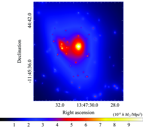
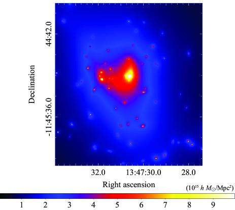
Figure 9: Surface mass density map of RX J1347.5–1145 measured with SL assuming two dark halo components (left) or three ones (right) in units of $10^{15}$ $h$ $M_{\odot}$ Mpc^-2. The entire morphology is nearly unchanged by an addition of the third dark matter component.

4.2 Gas stripping and sloshing

We find a clear offset between the mass peak of the subcluster and the position of the substructure in X-rays and the SZE (the bottom panels of Figure 10). The second mass peak is away from the peak position of the X-ray substructure with statistical significance of $5.5\sigma$. The second DM component is most likely associated with the infalling subcluster, suggesting that the gas that was originally in the subcluster is stripped by ram-pressure of the main cluster.

The top left panel of Figure 10 shows that the X-ray centroid coincides with the mass peak of the main cluster even though the ICM in the cool core is sloshing. The mass peak of the main cluster is located at the interface between the positive and the negative excesses of the dipolar pattern (see the bottom left panel of Figure 10). These features indicate that part of the gas in the cool core is moving around the BCG, but the DM distribution is not disturbed.

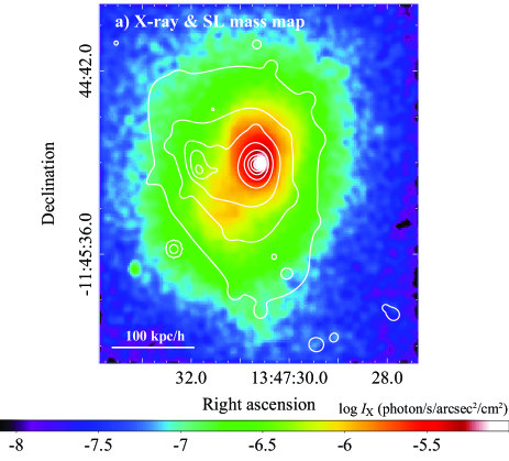
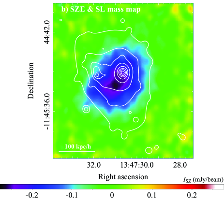
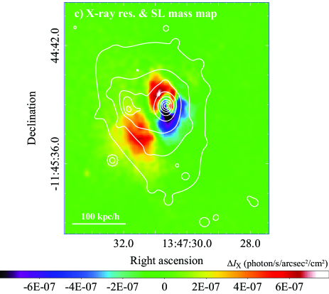
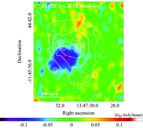
Figure 10: Comparison of morphology between the surface mass density map derived from two dark halo components and other wavelength images. Top left: White contours of the surface mass density map are overlaid on the X-ray surface brightness image. The contours indicate levels of 2.0, 3.0, 4.0, $\cdots$, 9.0, $10.0\times 10^{15}$ $h$ $M_{\odot}$ Mpc^-2, respectively. This X-ray image is the same as the left panel of Figure 1. The mass peak of the main cluster coincides with the X-ray centroid, while no X-ray counterparts are found at the mass peak of the subcluster. Top right: Same as the top left panel but for the SZE image. This SZE image is the same as the right panel of Figure 1. No SZE counterparts are found at the mass peak of the subcluster. Bottom left: Same as the top left panel but for the X-ray residual image. This X-ray residual image is the same as the left panel of Figure 2. The clear offset between the mass peak of the subcluster and the X-ray substructure is found. Bottom right: Same as the top left panel but for the SZE residual image. This SZE residual image is the same as the right panel of Figure 2. As shown in this top right panel, the offset between the SZE substructure and the mass peak of the subcluster is found.

5 Discussion

5.1 Origin of the excess hot ICM

The presence of very hot ICM in excess of 20 keV is inferred in RX J1347.5–1145 for the earlier SZE and X-ray observations (Kitayama et al., 2004; Ota et al., 2008). Combining the X-ray data of Chandra with the SZE data of ALMA, we have confirmed the temperature of the excess hot ICM by two independent methods and have improved precision of its position. The excess hot ICM is located at a distance of $27^{\prime\prime}$ (or $\sim 109\,h^{-1}$ kpc) to the southeast from the cluster center.

Following Section 3.4, we also measure the equation of state of the excess hot ICM. We compute $\Delta p$ and $\Delta\rho$ for an elliptical region with semi-major and semi-minor axis lengths of $14^{\prime\prime}$ and $12^{\prime\prime}$, respectively, and a position angle of $-70^{\circ}$ around the centroid of the excess SZE signal. We assume the line-of-sight depth of 150 kpc. Given that $\Delta I_{\rm X}>\langle I_{\rm X}\rangle$ in this region, we adopt $n_{\rm excess}$ given in Equation (2) as a better proxy for $\Delta\rho$ than Equation (4). On the other hand, $\Delta p$ is directly computed from the SZE residual signal, $\Delta I_{SZ}$. We analyze the X-ray spectrum in this region using the same procedure as described in Section 3.2. The electron number density and temperature of the excess hot ICM is $(3.29\pm 0.02)\times 10^{-2}$ cm^-3 and $20.2^{+2.1}_{-1.8}$ keV, respectively. We then find that the velocity inferred from the equation of state of the excess hot ICM is $1970\pm 150$ km s^-1, which matches $\sim 85$ % of the adiabatic sound speed of the 20 keV ICM, $\sim 2310$ km s^-1. This supports picture that the pressure perturbation in the southeast quadrant is induced by shock.

The excess hot ICM in the southeast quadrant is most likely associated with a major merger. The result of SL analysis indicates that the mass peak of the subcluster is offset from the location of the southeast substructure. Our results imply that the gas that was originally in the subcluster is stripped by ram-pressure of the main cluster. As mentioned above, the pressure perturbation of the southeast substructure in the SZE residual image is consistent with that created by shock, so it is plausible that this stripped gas has been heated during the major merger. Details of shock-heating processes in RX J1347.5–1145 using numerical simulations will be presented elsewhere.

5.2 Major merger and sloshing cool core

We have also found a dipolar pattern in the core of RX J1347.5–1145 in its X-ray residual image. This is direct evidence that the core is experiencing gas sloshing, whose presence was suggested before by Johnson et al. (2012) and Kreisch et al. (2016). We find that the ICM properties of the disturbed gas obtained by the X-ray spectral analysis are consistent with those expected by gas sloshing. In addition, we find that the equation of state of disturbed gas is consistent with being isobaric, i.e., the motion of gas sloshing is in pressure equilibrium. The morphology of this dipolar patter seems to be a spiral. If so, the direction of the sloshing motion is in the plane of the sky. Such dipolar spiral patterns are often found in local cool core clusters (e.g., Churazov et al., 2003; Clarke et al., 2004; Sanders et al., 2014; Ueda et al., 2017), which show no apparent feature of a major merger. Those indicate that their gas sloshing is induced by a minor merger. RX J1347.5–1145, however, has a subcluster and the excess hot ICM in its central 150 $h^{-1}$ kpc. RX J1347.5–1145 is therefore the first cluster ever known to host both a major merger and gas sloshing in the cool core.

The size of the dipolar pattern is a factor of $2\sim 3$ smaller than that often found in local cool core clusters (e.g., Ueda et al., 2017). Since the size tends to evolve with time after the passage of a subcluster (e.g., ZuHone et al., 2010), gas sloshing in this cluster is expected to have occurred recently. The dipolar spiral pattern indicates that the orbit of the major merger is in the plane of the sky. This is in accord with the fact that the redshift difference of the 2nd BCG from the BCG is less than 100 km s^-1 by optical observations (Lu et al., 2010). The stripped gas locates behind the subcluster, which indicates the infalling subcluster is in the first passage. It is unclear, however, whether or not the infalling subcluster is the origin of gas sloshing. If the direction of the passage is from southwest to northeast, it seems to be hard to disturb and create a rotational motion of the gravitational potential well of the main cluster. A possibility that the subcluster is in the first passage and gas sloshing is induced by another earlier merger, was suggested by Kreisch et al. (2016). In this paper, we can not constrain their scenario.

5.3 Self-interaction cross section for dark matter

As discussed above, it seems that the merger in RX J1347.5–1145 is in the plane of the sky. Following Markevitch et al. (2004), an offset in the positions of galaxies, DM halos, and the ICM allows us to constrain the self-interaction cross section of DM. We estimated the surface mass density of DM ($\Sigma_{s}$) in the subcluster using its mass distribution shown in the left panel of Figure 9. We measured the mean $\Sigma_{s}$ within a radius of 25 $h^{-1}$ kpc from the second mass peak. We also subtracted the contribution of the main cluster based on the parameters listed in Table 3. Assuming the scattering depth of $\tau_{s}=\Sigma_{s}\times\sigma_{\rm DM}/m<1$ for DM, we obtain the upper limit of the self-interaction cross section for DM to be $\sigma_{\rm DM}/m<2.1\,h^{-1}$ cm² g^-1, where $\sigma_{\rm DM}$ is the DM collision cross section and $m$ is the mass of a DM particle. To derive more conservative upper limit, we further considered the uncertainty of the surface mass density map of RX J1347.5–1145. We subtracted the $2\sigma$ value of the rms noise obtained in Section 4 from the original surface mass density map and re-estimated the cross section in the same manner as mentioned above. The $2\sigma$ (95% CL) upper limit of the cross section is then $\sigma_{\rm DM}/m<3.7\,h^{-1}$ cm² g^-1. The derived upper limits are comparable to those reported in the studies of other clusters (e.g., Markevitch et al., 2004; Harvey et al., 2015).

6 Conclusions

We have studied RX J1347.5–1145, one of the well-known major merging clusters, combining the high angular resolution, multi-wavelength data taken by Chandra, ALMA, and HST. The conclusions of this paper are summarized as follows.

• The residual image of the X-ray surface brightness shows a clear dipolar pattern in the cluster center, whereas, we find no excess SZE signal in the central region in the SZE residual image. The dipolar pattern indicates that a fraction of the gas in the cool core is disturbed by gas sloshing. We have estimated the equation of state of the perturbation in gas using the X-ray and SZE residual images. We find that the inferred velocity is $420^{+310}_{-420}$ km s^-1, which is much lower than the adiabatic sound speed of the 10 keV ICM inside the core; thus, the perturbation is consistent with being isobaric. This is the first direct evidence of sub-sonic nature of gas sloshing motion.

• Both X-ray and SZE residual images show an excess component in the southeast substructure. We find that the peak of excess hot ($\sim 30$ keV) ICM is located at $27^{\prime\prime}$ ($109\,h^{-1}$ kpc) to the southeast from the cluster center. This region is faint in X-rays but bright in the SZE. The X-ray inferred thermal pressure of the excess component is nearly constant among the regions where the SZE signal is prominent. The velocity inferred from the equation of state of the excess hot ICM is $1970\pm 150$ km s^-1, which is comparable to the adiabatic sound speed of the 20 keV ICM. This result supports a picture that the perturbation in the southeast is generated by shock.

• The mass distribution of RX J1347.5–1145 obtained with SL is reproduced well by the two dark halo components. Their mass peaks are in good agreement with the positions of the BCG and the 2nd BCG. The mass peak of the main cluster matches the X-ray centroid, while the mass peak of infalling subcluster is offset from the substructure in X-rays and the SZE. This indicates that the gas originated in the subcluster is stripped by ram-pressure of the main cluster and shock heated during an on-going major merger.

• In our scenario, this major merger is likely in the first passage. RX J1347.5–1145 is therefore an exceptional cluster in which the excess hot gas, on-going major merger, and the sloshing cool core coexist within the central $150$ $h^{-1}$ kpc.

• We have also constrained the self-interaction cross section of DM. The resulting upper limit of the cross section is $\sigma_{\rm DM}/m<3.7\,h^{-1}$ cm² g^-1 (95% CL).

References

- Adam et al. (2014) Adam, R., Comis, B., Macías-Pérez, J. F., et al. 2014, A&A, 569, A66
- Akahori & Yoshikawa (2008) Akahori, T., & Yoshikawa, K. 2008, PASJ, 60, L19
- Akahori & Yoshikawa (2010) —. 2010, PASJ, 62, 335
- Akahori & Yoshikawa (2012) —. 2012, PASJ, 64, 12
- Akamatsu & Kawahara (2013) Akamatsu, H., & Kawahara, H. 2013, PASJ, 65, 16
- Allen et al. (2002) Allen, S. W., Schmidt, R. W., & Fabian, A. C. 2002, MNRAS, 335, 256
- Anders & Grevesse (1989) Anders, E., & Grevesse, N. 1989, Geochim. Cosmochim. Acta, 53, 197
- Arnaud (1996) Arnaud, K. A. 1996, in Astronomical Society of the Pacific Conference Series, Vol. 101, Astronomical Data Analysis Software and Systems V, ed. G. H. Jacoby & J. Barnes, 17
- Ascasibar & Markevitch (2006) Ascasibar, Y., & Markevitch, M. 2006, ApJ, 650, 102
- Balucinska-Church & McCammon (1992) Balucinska-Church, M., & McCammon, D. 1992, ApJ, 400, 699
- Bertin & Arnouts (1996) Bertin, E., & Arnouts, S. 1996, A&AS, 117, 393
- Blanton et al. (2011) Blanton, E. L., Randall, S. W., Clarke, T. E., et al. 2011, ApJ, 737, 99
- Bourdin et al. (2013) Bourdin, H., Mazzotta, P., Markevitch, M., Giacintucci, S., & Brunetti, G. 2013, ApJ, 764, 82
- Bradač et al. (2008) Bradač, M., Schrabback, T., Erben, T., et al. 2008, ApJ, 681, 187
- Brunetti & Jones (2014) Brunetti, G., & Jones, T. W. 2014, International Journal of Modern Physics D, 23, 30007
- Churazov et al. (2016) Churazov, E., Arevalo, P., Forman, W., et al. 2016, MNRAS, 463, 1057
- Churazov et al. (2003) Churazov, E., Forman, W., Jones, C., & Böhringer, H. 2003, ApJ, 590, 225
- Clarke et al. (2004) Clarke, T. E., Blanton, E. L., & Sarazin, C. L. 2004, ApJ, 616, 178
- David & Kempner (2004) David, L. P., & Kempner, J. 2004, ApJ, 613, 831
- Feretti et al. (2012) Feretti, L., Giovannini, G., Govoni, F., & Murgia, M. 2012, A&A Rev., 20, 54
- Ferrari et al. (2011) Ferrari, C., Intema, H. T., Orrù, E., et al. 2011, A&A, 534, L12
- Fruscione et al. (2006) Fruscione, A., McDowell, J. C., Allen, G. E., et al. 2006, in Proc. SPIE, Vol. 6270, Society of Photo-Optical Instrumentation Engineers (SPIE) Conference Series, 62701V
- Garmire et al. (2003) Garmire, G. P., Bautz, M. W., Ford, P. G., Nousek, J. A., & Ricker, Jr., G. R. 2003, in Society of Photo-Optical Instrumentation Engineers (SPIE) Conference Series, Vol. 4851, Society of Photo-Optical Instrumentation Engineers (SPIE) Conference Series, ed. J. E. Truemper & H. D. Tananbaum, 28–44
- Gitti & Schindler (2004) Gitti, M., & Schindler, S. 2004, A&A, 427, L9
- Halkola et al. (2008) Halkola, A., Hildebrandt, H., Schrabback, T., et al. 2008, A&A, 481, 65
- Harvey et al. (2015) Harvey, D., Massey, R., Kitching, T., Taylor, A., & Tittley, E. 2015, Science, 347, 1462
- Hitomi Collaboration et al. (2018) Hitomi Collaboration, Aharonian, F., Akamatsu, H., et al. 2018, PASJ, 70, 9
- Inoue et al. (2016) Inoue, S., Hayashida, K., Ueda, S., et al. 2016, PASJ, 68, S23
- Itoh & Nozawa (2004) Itoh, N., & Nozawa, S. 2004, A&A, 417, 827
- Johnson et al. (2012) Johnson, R. E., Zuhone, J., Jones, C., Forman, W. R., & Markevitch, M. 2012, ApJ, 751, 95
- Kalberla et al. (2005) Kalberla, P. M. W., Burton, W. B., Hartmann, D., et al. 2005, A&A, 440, 775
- Kawamata et al. (2016) Kawamata, R., Oguri, M., Ishigaki, M., Shimasaku, K., & Ouchi, M. 2016, ApJ, 819, 114
- Khatri & Gaspari (2016) Khatri, R., & Gaspari, M. 2016, MNRAS, 463, 655
- Kitayama et al. (2004) Kitayama, T., Komatsu, E., Ota, N., et al. 2004, PASJ, 56, 17
- Kitayama et al. (2016) Kitayama, T., Ueda, S., Takakuwa, S., et al. 2016, PASJ, 68, 88
- Köhlinger & Schmidt (2014) Köhlinger, F., & Schmidt, R. W. 2014, MNRAS, 437, 1858
- Komatsu et al. (1999) Komatsu, E., Kitayama, T., Suto, Y., et al. 1999, ApJ, 516, L1
- Komatsu et al. (2001) Komatsu, E., Matsuo, H., Kitayama, T., et al. 2001, PASJ, 53, 57
- Korngut et al. (2011) Korngut, P. M., Dicker, S. R., Reese, E. D., et al. 2011, ApJ, 734, 10
- Kreisch et al. (2016) Kreisch, C. D., Machacek, M. E., Jones, C., & Randall, S. W. 2016, ApJ, 830, 39
- Lu et al. (2010) Lu, T., Gilbank, D. G., Balogh, M. L., et al. 2010, MNRAS, 403, 1787
- Markevitch et al. (2004) Markevitch, M., Gonzalez, A. H., Clowe, D., et al. 2004, ApJ, 606, 819
- Markevitch et al. (2002) Markevitch, M., Gonzalez, A. H., David, L., et al. 2002, ApJ, 567, L27
- Markevitch et al. (2001) Markevitch, M., Vikhlinin, A., & Mazzotta, P. 2001, ApJ, 562, L153
- Mason et al. (2010) Mason, B. S., Dicker, S. R., Korngut, P. M., et al. 2010, ApJ, 716, 739
- McMullin et al. (2007) McMullin, J. P., Waters, B., Schiebel, D., Young, W., & Golap, K. 2007, in Astronomical Society of the Pacific Conference Series, Vol. 376, Astronomical Data Analysis Software and Systems XVI, ed. R. A. Shaw, F. Hill, & D. J. Bell, 127
- Meneghetti et al. (2017) Meneghetti, M., Natarajan, P., Coe, D., et al. 2017, MNRAS, 472, 3177
- Navarro et al. (1997) Navarro, J. F., Frenk, C. S., & White, S. D. M. 1997, ApJ, 490, 493
- Nevalainen et al. (2010) Nevalainen, J., David, L., & Guainazzi, M. 2010, A&A, 523, A22
- Oguri (2010) Oguri, M. 2010, PASJ, 62, 1017
- Oguri et al. (2012) Oguri, M., Bayliss, M. B., Dahle, H., et al. 2012, MNRAS, 420, 3213
- Ota et al. (2008) Ota, N., Murase, K., Kitayama, T., et al. 2008, A&A, 491, 363
- Plagge et al. (2013) Plagge, T. J., Marrone, D. P., Abdulla, Z., et al. 2013, ApJ, 770, 112
- Planck Collaboration et al. (2016) Planck Collaboration, Ade, P. A. R., Aghanim, N., et al. 2016, A&A, 594, A27
- Reese et al. (2010) Reese, E. D., Kawahara, H., Kitayama, T., et al. 2010, ApJ, 721, 653
- Ricker & Sarazin (2001) Ricker, P. M., & Sarazin, C. L. 2001, ApJ, 561, 621
- Riess et al. (2016) Riess, A. G., Macri, L. M., Hoffmann, S. L., et al. 2016, ApJ, 826, 56
- Roediger & Brüggen (2007) Roediger, E., & Brüggen, M. 2007, MNRAS, 380, 1399
- Roediger et al. (2011) Roediger, E., Brüggen, M., Simionescu, A., et al. 2011, MNRAS, 413, 2057
- Sanders et al. (2014) Sanders, J. S., Fabian, A. C., Hlavacek-Larrondo, J., et al. 2014, MNRAS, 444, 1497
- Sasaki et al. (2016) Sasaki, T., Matsushita, K., Sato, K., & Okabe, N. 2016, PASJ, 68, 85
- Schellenberger et al. (2015) Schellenberger, G., Reiprich, T. H., Lovisari, L., Nevalainen, J., & David, L. 2015, A&A, 575, A30
- Schindler et al. (1997) Schindler, S., Hattori, M., Neumann, D. M., & Boehringer, H. 1997, A&A, 317, 646
- Sunyaev & Zeldovich (1972) Sunyaev, R. A., & Zeldovich, Y. B. 1972, Comments on Astrophysics and Space Physics, 4, 173
- Takizawa (2005) Takizawa, M. 2005, ApJ, 629, 791
- Takizawa (2006) —. 2006, PASJ, 58, 925
- Ueda et al. (2017) Ueda, S., Kitayama, T., & Dotani, T. 2017, ApJ, 837, 34
- van Weeren et al. (2017) van Weeren, R. J., Andrade-Santos, F., Dawson, W. A., et al. 2017, Nature Astronomy, 1, 0005
- Zitrin et al. (2015) Zitrin, A., Fabris, A., Merten, J., et al. 2015, ApJ, 801, 44
- ZuHone et al. (2010) ZuHone, J. A., Markevitch, M., & Johnson, R. E. 2010, ApJ, 717, 908