Neural Task Planning with
And-Or Graph Representations

Abstract

This paper focuses on semantic task planning, i.e., predicting a sequence of actions toward accomplishing a specific task under a certain scene, which is a new problem in computer vision research. The primary challenges are how to model task-specific knowledge and how to integrate this knowledge into the learning procedure. In this work, we propose training a recurrent long short-term memory (LSTM) network to address this problem, i.e., taking a scene image (including pre-located objects) and the specified task as input and recurrently predicting action sequences. However, training such a network generally requires large numbers of annotated samples to cover the semantic space (e.g., diverse action decomposition and ordering). To overcome this issue, we introduce a knowledge and-or graph (AOG) for task description, which hierarchically represents a task as atomic actions. With this AOG representation, we can produce many valid samples (i.e., action sequences according to common sense) by training another auxiliary LSTM network with a small set of annotated samples. Furthermore, these generated samples (i.e., task-oriented action sequences) effectively facilitate training of the model for semantic task planning. In our experiments, we create a new dataset that contains diverse daily tasks and extensively evaluate the effectiveness of our approach.

I Introduction

Automatically predicting and executing a sequence of actions given a specific task is an ability that is quite expected for intelligent robots [1, 2]. For example, to complete the task of “make tea” under the scene shown in Figure 1, an agent needs to plan and successively execute a number of steps, e.g., “move to the tea box” and “grasp the tea box”. In this paper, we aim to train a neural network model to enable this capability, which has rarely been addressed in computer vision research.

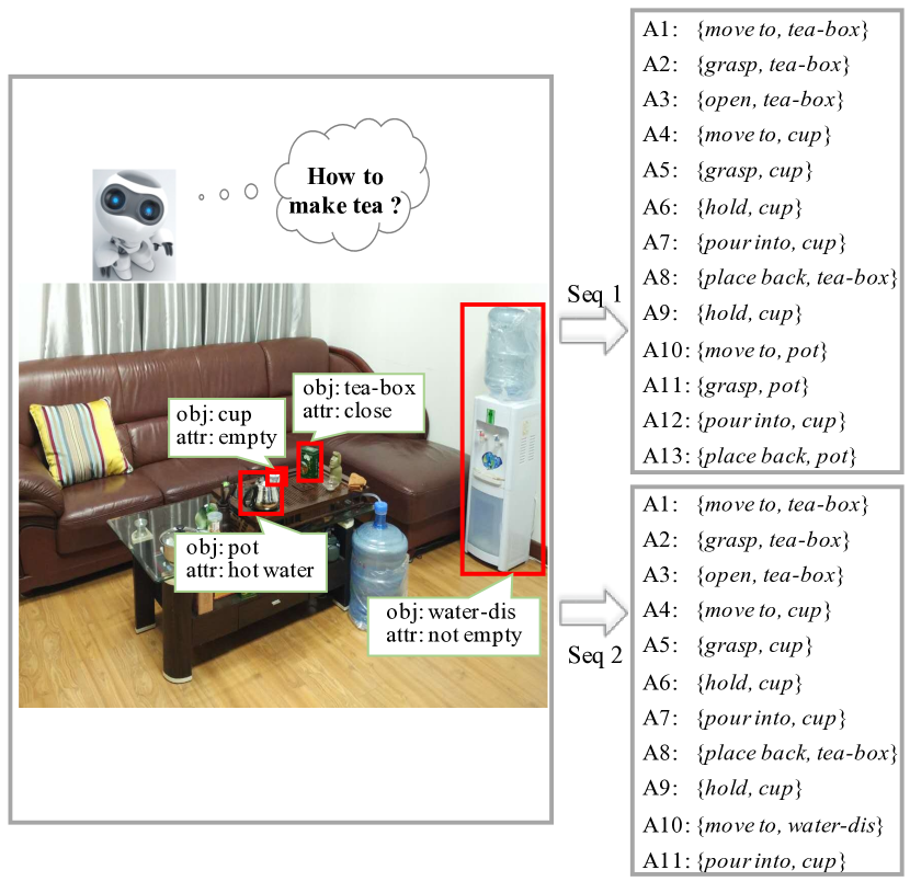
Figure 1: Two alternative action sequences, inferred according to the joint understanding of the scene image and task semantics, for completing the task “make tea” under a given office scene. An agent can achieve this task by successively executing either of the sequences.

We regard the aforementioned problem as semantic task planning, i.e., predicting a sequence of atomic actions toward accomplishing a specific task. Furthermore, we consider an atomic action to be a primitive action operating on an object, denoted by a two-tuple $A=(action,object)$. Therefore, the prediction of action sequences depends on not only the task semantics (i.e., how the task is represented and planned) but also the visual scene image parsing (e.g., recognizing object categories, states and their spatial relations in the scene). Considering the task of a robot pouring a cup of water from a pot, the predicted sequence varies according to the properties of the objects in the scene such as the relative distances among the agent, cup and pot and the state of the cup (empty or not). If the robot is located far from the cup, it should first move close to the cup and then grasp the cup. If the cup is full of water, the robot will have to pour the water out before filling the cup with water from the pot. Since recent advanced deep convolutional neural networks (CNNs) [3, 4, 5, 6] have achieved great successes in object categorization [7, 8, 9, 10, 11, 12, 13] and localization [14, 15, 16, 17], we assume that objects are correctly located and that the initial states of the objects are known in the given scene in this work. However, this problem remains challenging due to the diversity of action decomposition and ordering, long-term dependencies among atomic actions, and large variations in object states and layouts in the scene.

In this work, we develop a recurrent long short-term memory (LSTM) [18] network to address the problem of semantic task planning because LSTM networks have been demonstrated to be effective in capturing long-range sequential dependencies, especially for tasks such as machine translation [19] and image/video captioning [20, 21]. These approaches generally adopt an encoder-decoder architecture, in which an encoder first encodes the input data (e.g., an image) into a semantic-aware feature representation and a decoder then decodes this representation into the target sequence (e.g., a sentence description). In this work, we transform the input image into a vector that contains the information about the object categories and locations and then feed this vector into the LSTM network (named Action-LSTM) with the specified task. This network is capable of generating the action sequence through the encoder-decoder learning.

In general, large numbers of annotated samples are required to train LSTM networks, especially for complex problems such as semantic task planning. To overcome this issue, we present a two-stage training method by employing a knowledge and-or graph (AOG) representation [22, 23, 24]. First, we define the AOG for task description, which hierarchically decomposes a task into atomic actions according to their temporal dependencies. In this semantic representation, an and-node represents the chronological decomposition of a task (or sub-task), an or-node represents the alternative ways to complete the certain task (or sub-task), and leaf nodes represent the pre-defined atomic actions. The AOG can thus contain all possible action sequences for each task by embodying the expressiveness of grammars. Specifically, given a scene image, a specific action sequence can be generated by selecting the sub-branches at all of the or-nodes in a depth-first search (DFS) manner. Second, we train an auxiliary LSTM network (named AOG-LSTM) to predict the selection at the or-nodes in the AOG and thus produce a large number of new valid samples (i.e., task-oriented action sequences) that can be used for training the Action-LSTM network. Notably, training the AOG-LSTM network requires only a few manually annotated samples (i.e., scene images and the corresponding action sequences) because making a selection in the context of task-specific knowledge (represented by the AOG) is seldom ambiguous.

Note that a preliminary version of this work has been presented at a conference [25]. In this paper, we inherit the idea of integrating task-specific knowledge via a two-stage training method, and we extend the initial version from several aspects to strengthen our method. First, we extend the benchmark to involve more tasks and include more diverse scenarios. Moreover, because the automatically augmented set includes some difficult samples with uncertain and even incorrect labels, we further incorporate curriculum learning [26, 27] to address this issue by starting the training with only easy samples and then gradually extending to more difficult samples. Finally, more detailed comparisons and analyses are conducted to demonstrate the effectiveness of our proposed model and to verify the contribution of each component.

The main contributions of this paper are two-fold. First, we present a new problem called semantic task planning and create a benchmark (that includes 15 daily tasks and 1,284 scene images). Second, we propose a general approach for incorporating complex semantics into the recurrent neural network (RNN) learning, which can be generalized to various high-level intelligent applications.

The remainder of this paper is organized as follows. Section II provides a review of the most-related works. Section III presents a brief overview of the proposed method. We then introduce the AOG-LSTM and Action-LSTM modules in detail in Sections IV and V, respectively, with thorough analyses of the network architectures, training and inference processes of these two modules. Extensive experimental results, comparisons and analyses are presented in Section VI. Finally, Section VII concludes this paper.

II Related work

We review the related works following three main research streams: task planning, action recognition and prediction, and recurrent sequence prediction.

II-A Task planning

In the literature, task planning (also referred to as symbolic planning [28]) has traditionally been formalized as deduction [29, 30] or satisfiability [31, 32] problems for long periods. Sacerdoti et al. [33] introduced hierarchical planning, which first performed planning in an abstract manner and then generated fine-level details. Yang et al. [34] utilized the standard Planning Domain Definition Language (PDDL) representation for actions and developed an action-related modeling system to learn an action model from a set of observed successful plans. Some work also combined symbolic planning with motion planning [35]. Cambon et al. [36] regarded symbolic planning as a constraint and proposed a heuristic function for motion planning. Plaku et al. [37] extended the work and planned using geometric and differential constraints. Wolfe et al. [38] proposed a hierarchical task and motion planning algorithm based on hierarchical transition networks. Although those algorithms performed quite well in controlled environments, they required encoding every precondition for each operation or domain knowledge, and they can hardly be generalized to unconstrained environments with large variances [28]. Recently, Sung et al. [28, 39] represented an environment with a set of attributes and proposed using a Markov random field (MRF) [40] to learn the sequences of controllers to complete the given tasks. Xiong et al. [23] developed a stochastic graph-based framework, which incorporated spatial, temporal and causal knowledge, for a robot to understand tasks, and they successfully applied this framework to a cloth-folding task.

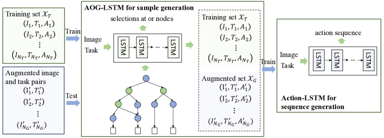
Figure 2: An overall introduction of the proposed method. The AOG-LSTM network is trained using the samples from the small training set, and it can be used to generate a relatively large augmented set. The augmented set, together with the training set, is used to train the Action-LSTM network, which can directly predict the action sequence to complete a given task under a certain scene.

Some other works also manually defined the controller sequences for completing certain tasks, including baking cookies [41], making pancakes [42], and folding laundry [43]. In these works, the controller sequences were selected from several predefined sequences or retrieved from a website. For example, in the work [42], the robot retrieved instructions for making pancakes from the Internet to generate the controller sequence. Although they often achieve correct sequences in controlled environments, these methods cannot scale up to a large number of tasks in unconstrained household environments because each task requires defining complicated rules for the controller sequence to adapt to various environments.

Recently, a series of works [44, 45] developed learning-based planners for semantic visual planning tasks. Gupta et al. [45] proposed a cognitive mapper and planner for visual navigation, therein constructing a top-down belief map of the world and applying a differentiable neural network planner to produce the next action at each time step. Zhu et al. [44] formulated visual semantic planning as a policy learning problem and proposed an interaction-centric solution that offered crucial transferability properties for semantic action sequence prediction. In addition to visual semantic planning, the deep neural networks were also adopted to address the tasks of robotic control planning [46, 47, 48]. For example, Agrawal et al. [47] developed a joint forward and inverse models for real-world robotic manipulation tasks. The inverse model provided supervision to construct informative visual features, which the forward model then predicted and in turn regularized the feature space for the inverse model. Pascanu et al. [46] introduced an imagination-based planner that could learn to construct, evaluate, and execute plans.

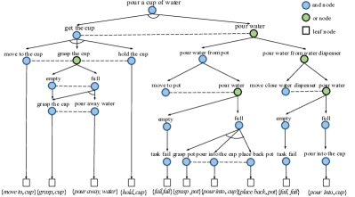
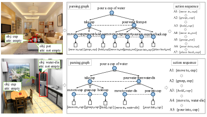
Figure 3: An example of a knowledge and-or graph for describing the task “pour a cup of water” shown in (a) and two parsing graphs and their corresponding action sequences under two specific scenes shown in (b).

II-B Action recognition and prediction

The problem studied in this paper is also related to action recognition and prediction, where the former attempts to recognize action categories performed by persons from a fully observed video/image [49, 50, 51, 52, 53] and the latter targets predicting an action that humans are likely to perform in the future within given scenarios [54, 55, 56]. Note that our work differs from the aforementioned methods in the goal of the problem, which is to automatically infer potential action sequences that can be used to complete the task at hand in the specific environment. Note that action recognition and prediction can be beneficial to our work because they provide a better understanding of the interaction between humans and the environment for the robots for task planning.

II-C Recurrent sequence prediction

RNNs [57], particularly LSTM [18], were developed for modeling long-term temporal dependencies. Recently, RNNs have been extensively applied to various sequence prediction tasks, including natural language generation [58, 59, 60], neural machine translation [19, 61, 62, 63], and image and video captioning [20, 64, 65, 66, 21]. These works adopted a similar encoder-decoder architecture for solving sequence prediction. Tang et al. [60] encoded the contexts into a continuous semantic representation and then decoded the semantic representation into context-aware text sequences using RNNs. Cho et al. [19] mapped a free-form source language sentence into the target language by utilizing the encoder-decoder recurrent network. Vinyals et al. [20] applied a similar pipeline for image captioning, therein employing a CNN as the encoder to extract image features and an LSTM network as the decoder to generate the descriptive sentence. Pan et al. [66] further adapted this pipeline to video caption generation by developing a hierarchical recurrent neural encoder that is capable of efficiently exploiting the video temporal structure in a longer range to extract video representations.

III Overview

In this section, we give an overall introduction to the proposed method. First, we represent the possible action sequences for each task with an AOG. Based on this AOG, a parsing graph, which corresponds to a specific action sequence, can be generated by selecting the sub-branches at all the or-nodes searched in a DFS manner given a scene image. An LSTM (namely, AOG-LSTM) is learned to make predictions at these or-nodes given a large number of new scene image and automatically produce a relatively large number of valid samples. Finally, these automatically generated samples are used to train another LSTM (namely, Action-LSTM) that directly predicts the action sequence to complete a given task under a certain scene. An overall illustration is presented in Figure 2.

IV Semantic Task Representation

IV-A Atomic action definition

An atomic action refers to a primitive action operating on an associated object, and it is denoted as a two-tuple set $A=(action,object)$. To ensure that the learned model can generalize across different tasks, the primitive action and associated object should satisfy two properties [39]: 1) each primitive action should specialize an atomic operation, such as open, grasp or move to, and 2) the primitive actions and associated objects should not be specific to one task. With these role-specific and generalizable settings, large numbers of high-level tasks can be completed using the atomic actions defined on a small set of primitive actions and associated objects. In this work, $B_{a}=$12 primitive actions and $B_{o}=$12 objects are involved, as described in Section VI-A.

IV-B Knowledge and-or graph

The AOG is defined as a 4-tuple set $\mathcal{G}=\{S,V_{N},V_{T},P\}$, where $S$ is the root node denoting a task. The non-terminal node set $V_{N}$ contains both and-nodes and or-nodes. An and-node represents the decomposition of a task to its sub-tasks in chronological order. An or-node is a switch, deciding which alternative sub-task to select. Each or-node has a probability distribution $\mathbf{p}_{t}$ (the $t$-th element of $P$) over its child nodes, and the decision is made based on this distribution. $V_{T}$ is the set of terminal nodes. In our definition of AOG, the non-terminal nodes refer to the sub-tasks and atomic actions, and the terminal nodes associate a batch of atomic actions. In this work, we manually define the structure of the AOG for each task.

According to this representation, the task “pour a cup of water” can be represented as the AOG shown in Figure 3(a). The root node denotes the task, where is first decomposed into two sub-tasks, i.e., “get the cup” and “pour water”, under the temporal constraint. The “get the cup” node is an and-node and can be further decomposed into “move to the cup”, “take the cup” and “hold the cup” in chronological order. The “pour water” node is an or-node, and it has two alternative sub-branches, i.e., “pour water from the water dispenser” and “pour water from the pot”. Finally, all the atomic actions are treated as the primitive actions and associated objects, which are represented by the terminal nodes. In this way, the knowledge AOG contains all possible action sequences of the corresponding task in a syntactic manner.

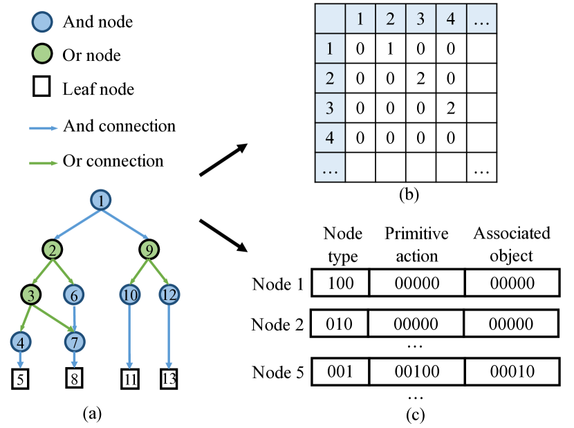
Figure 4: Illustration of the AOG encoding process. The nodes in the AOG are first numbered (a). Then, an adjacency matrix is employed to encode the structure of the graph, with a value of 1 for an and connection, 2 for an or connection and 0 otherwise (b). The content of each node contains a one-hot vector denoting the node type, two one-hot vectors representing the primitive action and the associated object of the associated atomic action for the leaf node, and two zero vectors for the and- and or-nodes.

IV-C Sample generation with and-or graph

In addition to capturing the task semantics, the AOG representation enables the generation of a large number of valid samples (i.e., action sequences extracted from the AOG), which are important for the RNN learning process. According to the definition of the AOG, a parsing graph, which corresponds to a specific action sequence (e.g., Figure 3(b)), will be generated by selecting the sub-branches for all the or-nodes searched in a DFS manner given a new scene image. Since explicit temporal dependencies exist among these or-nodes, we can recurrently activate these selections using an LSTM network, i.e., AOG-LSTM.

AOG encoding. Before discussing the AOG-LSTM, we first introduce how to encode the AOG into a feature vector because this is a crucial process for integrating the AOG representation into the LSTM. Concretely, the AOG features should contain both graph structure and node content information, and the encoding process consists of three steps, as illustrated in Figure 4. First, we number all the nodes in the AOG, as shown in Figure 4(a). Second, an adjacency matrix [67] is utilized to encode the graph structure that depicts whether and how two nodes are connected. Consistent with the situation whereby and- and or-nodes exist in the AOG and they represent completely different meanings, we define an and connection to signify a connection of an and-node to its child and an or connection to signify that of an or-node to its child. Suppose that the adjacency matrix is $M$, with $M_{ij}$ being the value of row $i$ and column $j$; $M_{ij}$ is set to 1 for the and connection of the and-node $i$ to its child $j$, 2 for the or connection and 0 otherwise (see Figure 4(b)). Third, we extract the features for each node to encode its node type and related atomic action information. There are three types of nodes in the AOG, i.e., and, or and leaf nodes, and we utilize one-hot vectors to represent these nodes. As indicated in the definition of the AOG, a leaf node is connected to a specific atomic action, and we employ two one-hot vectors to represent the primitive action and associated object of the atomic action. Then, we append the two vectors after the node type vector to obtain the features of this node. In contrast, the and- and or-nodes do not connect to the specific atomic action directly; thus, we simply pad zeros after the node type vector (see Figure 4(c)). Finally, the adjacency matrices are re-arranged to a vector, and the vector is concatenated with all the node features to achieve the final representation of the AOG.

According to the AOG definition, we search the or-nodes based on the depth-first and from left-to-right manner. As illustrated in Figure 5, our model first extracts the features of the given scene image and the task, and it maps them to a feature vector, which serves as the initial hidden state of the AOG-LSTM. The model then encodes the initial AOG as a feature vector, which is fed into the AOG-LSTM to predict the sub-branch selection of the first or-node. Meanwhile, the AOG is updated by pruning the unselected sub-branches. Note that the AOG is updated based on the annotated and predicted selections during the training and test stages, respectively. Based on the updated AOG, the same process is conducted to predict the selection of the second or-node. This process is repeated until all or-nodes have been visited, and a parsing graph is then constructed. We denote the image and task features as $\mathbf{f}^{I}$ and $\mathbf{f}^{T}$, respectively, and we denote the AOG features at time step $t$ as $\mathbf{f}_{t}^{AOG}$. The prediction at time step $t$ can be expressed as follows:

$$\begin{split}&\mathbf{f}_{IT}=[\mathrm{relu}(\mathbf{W}_{fI}\mathbf{f}^{I}),\mathrm{relu}(\mathbf{W}_{fT}\mathbf{f}^{T})]\\ &\mathbf{c}_{0}=\mathbf{0};\ \mathbf{h}_{0}=\mathbf{W}_{hf}\mathbf{f}_{IT}\\ &[\mathbf{h}_{t},\mathbf{c}_{t}]=\mathrm{LSTM}(\mathbf{f}^{AOG}_{t},\mathbf{h}_{t-1},\mathbf{c}_{t-1})\\ &\mathbf{p}_{t}=\mathrm{softmax}(\mathbf{W}_{hp}\mathbf{h}_{t}+\mathbf{b}_{p})\end{split}$$ (1)

where $\mathrm{relu}$ is the rectified linear unit (ReLU) function [68] and $\mathbf{p}_{t}$ is the probability distribution over all child branches of the $t$-th or-node, where the branch with the maximum value is selected. $\mathbf{W}_{fI}$, $\mathbf{W}_{fT}$, $\mathbf{W}_{hf}$, and $\mathbf{W}_{hp}$ are the parameter matrices, and $\mathbf{b}_{p}$ is the corresponding bias vector. $\mathbf{f}^{I}$ are the image features containing the information of the class labels, initial states, and locations of the objects in image $I$. More concretely, suppose that there are $B_{o}$ categories of objects and $k$ attributes. For each object in an given image, we utilize a $B_{o}$-dimension one-hot vector to denote its class label information, $k$ vectors to denote the initial states of the $k$ attributes, and a 4-dimension vector to denote the bounding box of the object region. Thus, each object can be represented by a fixed dimension feature vector, and the feature vectors of all objects are concatenated to obtain an image feature vector. However, the number of objects varies in different images, leading to image feature vectors with different dimensions. To address this issue, we first extract the features for the image with the maximum number of objects, and we apply zero padding to each feature vector so that each vector has the same dimensions as the feature vector of the image with the maximum number of objects. $\mathbf{f}^{T}$ is a one-hot vector denoting a specific task. $\mathbf{f}^{I}$ and $\mathbf{f}^{T}$ are first processed using two separated fully connected layers followed by the ReLU function to generate two 256-D feature vectors. The initial memory cell $\mathbf{c}_{0}$ is set as a zero vector. The two vectors are then concatenated and mapped to a 256-D feature vector using a fully connected layer, which serves as the initial hidden state of the LSTM. $\mathbf{f}^{AOG}_{t}$ are the AOG feature vectors at time step $t$, which are also pre-processed to a 256-D feature vector via a fully connected layer and then fed to the AOG-LSTM. The size of the hidden layer of the LSTM is 256 neurons.

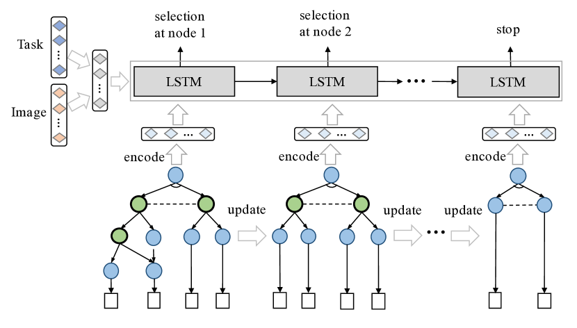
Figure 5: The AOG-LSTM architecture for selecting the sub-branches at all of the or-nodes in a knowledge and-or graph.

AOG-LSTM training. Making a selection at the or-nodes is less ambiguous because the AOG representation effectively regularizes the semantic space. Thus, we can train the AOG-LSTM using only a small number of annotated samples. Specifically, we collect a small set of samples annotated with the selections of all or-nodes given a scene image for each task, i.e., $\mathcal{X}_{T}=\{I_{n},T_{n},\mathbf{s}_{n}\}_{n=1}^{N_{T}}$, in which $I_{n}$ and $T_{n}$ are the $n$-th given image and task, respectively, and $\mathbf{s}_{n}=\{s_{n1},s_{n2},\dots,s_{n{K_{n}}}\}$ is a set whereby $s_{nb}$ denotes the selection for the $t$-th or-node and $K_{n}$ is the number of or-nodes. $N_{T}$ is the number of annotated samples in $\mathcal{X}_{T}$. Given the predicted probability $\mathbf{p}_{nt}=\{p_{nt1},p_{nt2},\dots,p_{ntB}\}$ for the $t$-th or-node, we define the objective function as the sum of the negative log-likelihood of correct selections over the entire training set, which is formulated as

$$\mathcal{L}_{aog}=-\sum_{n=1}^{N_{T}}\sum_{t=1}^{K_{n}}\sum_{b=0}^{B}{\mathbf{1}(s_{nb}=b)\log{p_{ntb}}},$$ (2)

where $\mathbf{1}(\cdot)$ is an indicator function whose value is 1 when the expression is true and 0 otherwise and $B$ is the number of sub-branches. In our experiment, because the maximum number of sub-branches is 3, we simply set $B$ to 3.

Sample generation. Once the AOG-LSTM is trained, we use it to predict the sub-branch selections for all the or-nodes in the AOG given different scene images and generate the corresponding action sequences. In this way, a relatively large set of $\mathcal{X}_{G}=\{I_{n},T_{n},\mathcal{A}_{n}\}_{n=1}^{N_{G}}$ is obtained, where $I_{n}$, $T_{n}$, and $\mathcal{A}_{n}$ represent the image, task and predicted sequence for the $n$-th sample, respectively, and $N_{G}$ is the number of generated samples. More importantly, it can also generate samples of unseen tasks using an identical process in which the AOG structures for the new tasks are also manually defined. These newly generated samples effectively alleviate the problem of manually annotating large numbers of samples in practice.

V Recurrent action prediction

We formulate the problem of semantic task planning in the form of the probability estimation $p(A_{1},A_{2},...,A_{n}|I,T)$, where $I$ and $T$ are the given scene image and the task, respectively, and $\{A_{1},A_{2},...,A_{n}\}$ denotes the predicted sequence. Based on the chain rule, the probability can be recursively decomposed as follows:

$$p(A_{1},A_{2},...,A_{n}|I,T)=\prod_{t=1}^{n}p(A_{t}|I,T,\mathcal{A}_{t-1}),$$ (3)

where $\mathcal{A}_{t-1}$ denotes $\{A_{1},A_{2},...,A_{t-1}\}$ for convenience of illustration. The atomic action is defined as $A_{i}=(a_{i},o_{i})$. Since an atomic action is composed of a primitive action and an associated object, there are large numbers of atomic actions that have few samples because action-object co-occurrence is infrequent in the training samples. Thus, a fundamental problem in atomic action prediction is learning from very few samples. Fortunately, although the atomic action might occur rarely in the samples, its primitive action and associated object independently appear quite frequently. Thus, in this work, we simplify the model by assuming independence between the primitive actions and the associated objects and predict them separately [69]. The probability can be expressed as follows:

$$p(A_{t}|I,T,\mathcal{A}_{t-1})=p(a_{t}|I,T,\mathcal{A}_{t-1})p(o_{t}|I,T,\mathcal{A}_{t-1}).$$ (4)

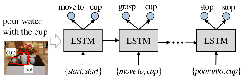
Figure 6: The Action-LSTM architecture for predicting the atomic action sequence given a specific task.

Here, we develop the Action-LSTM network to model the probability distribution, i.e., equation (3). Specifically, the Action-LSTM network first applies a process similar to that of AOG-LSTM to extract the features of the task and image, which is also used to initialize the hidden state of the LSTM. At each time step $t$, two softmax layers are utilized to predict the probability distributions $\mathbf{p}(a_{t})$ over all primitive actions and $\mathbf{p}(o_{t})$ over all associated objects. The conditions on the previous $t-1$ actions can be expressed by the hidden state $h_{t-1}$ and memory cell $c_{t-1}$. The action prediction at time step $t$ can be computed as follows:

$$\begin{split}&\mathbf{f}_{IT}=[\mathrm{relu}(\mathbf{W}_{fI}\mathbf{f}^{I}),\mathrm{relu}(\mathbf{W}_{fT}\mathbf{f}^{T})]\\ &\mathbf{c}_{0}=\mathbf{0};\ \mathbf{h}_{0}=\mathbf{W}_{hf}\mathbf{f}_{IT}\\ &[\mathbf{h}_{t},\mathbf{c}_{t}]=\mathrm{LSTM}(\mathbf{f}^{A}_{t},\mathbf{h}_{t-1},\mathbf{c}_{t-1})\\ &\mathbf{p}(a_{t})=\mathrm{softmax}(\mathbf{W}_{ah}\mathbf{h}_{t}+\mathbf{b}_{a})\\ &\mathbf{p}(o_{t})=\mathrm{softmax}(\mathbf{W}_{oh}\mathbf{h}_{t}+\mathbf{b}_{o})\end{split}$$ (5)

where $\mathrm{relu}$ is the ReLU function. $\mathbf{W}_{fI}$, $\mathbf{W}_{fT}$, $\mathbf{W}_{hf}$, $\mathbf{W}_{ah}$, and $\mathbf{W}_{oh}$ are the parameter matrices, and $\mathbf{b}_{a}$ and $\mathbf{b}_{o}$ are the corresponding bias vectors. Figure 6 presents an illustration of the Action-LSTM network. $\mathbf{f}^{I}$ and $\mathbf{f}^{T}$ carry exactly the same information as explained for the AOG-LSTM, and they are pre-processed using an identical process except that the last fully connected layer has 512 output neurons and thus generates a 512-D feature vector. Additionally, this feature vector is considered to be the initial hidden state of the Action-LSTM. $\mathbf{f}^{A}_{t}$ is a feature vector that encodes the input atomic action at time step $t$, which is concatenated by two one-hot vectors denoting its primitive action and associated object. Note that the atomic action is the ground truth and predicted atomic action of the previous time step during the training and test stages, respectively. Because directly predicting the atomic action is considerably more complicated, we set the size of the hidden layer of the LSTM to 512 neurons.

Action-LSTM training. In the training stage, we leverage the entire training set, including the manually annotated samples and the automatically generated samples, to optimize the network. However, some difficult samples with uncertain or even incorrect labels exist, and these samples may severely impact the model convergence and lead to inferior results. Meanwhile, skipping too many difficult training samples leads to a risk of overfitting on the small set of easy samples, resulting in a poor generalization ability to unseen testing data. To strike a better balance, we employ a curriculum learning algorithm [26, 27] that starts the training process using the most reliable samples and then gradually increases the sample difficulty.

To determine the difficulty of a particular sample, we consider the uncertainty of making selections at the or-nodes during the sample generation stage. Concretely, a probability distribution is predicted when performing selections at an or-node, and the entropy of this distribution well measures the uncertainty [70, 71]. Thus, we define the uncertainty of a sample by averaging the entropies of the predicted distributions over all the or-nodes. In this way, a sample having a higher uncertainty means that it is more difficult. We create a curriculum of $X_{G}$ by sorting the samples according to their uncertainty values and set a threshold $\tau$ to exclude the samples with uncertainty values that are higher than $\tau$. The curriculum is updated by decreasing $\tau$ to include more difficult samples during the training stage.

Formally, we are given the manually annotated and automatically generated sets, i.e., $\mathcal{X}_{T}=\{I_{n},T_{n},\mathcal{A}_{n}\}_{n=1}^{N_{T}}$ and $\mathcal{X}_{G}=\{I_{n},T_{n},\mathcal{A}_{n}\}_{n=1}^{N_{G}}$, where $I_{n}$ and $T_{n}$ are the given image and task of the $n$-th sample, respectively, and $\mathcal{A}_{n}=\{A_{n1},A_{n2},...,A_{n{W_{n}}}\}$ is the atomic action sequence, with $W_{n}$ denoting the number of atomic actions. $A_{nt}=\{a_{nt},o_{nt}\}$ is the $t$-th atomic action, with $a_{nt}$ and $o_{nt}$ denoting its primitive action and associated object, respectively. Similarly, we define the objective function as the sum of the negative log-likelihood of correct sequences over all the samples in the manually annotated set and the selected samples in the automatically generated set. Given the predicted distribution of the primitive action $\mathbf{p}_{n}(a_{t})=\{p_{n1}(a_{t}),p_{n2}(a_{t}),\dots,p_{n{B_{a}}}(a_{t})\}$ and associated object $\mathbf{p}_{n}(o_{t})=\{p_{n1}(o_{t}),p_{n2}(o_{t}),\dots,p_{n{B_{o}}}(o_{t})\}$ for the $t$-th step, the objective function can be expressed as

$$\mathcal{L}_{action}=-\sum_{n=1}^{N_{T}}\sum_{t=1}^{W_{n}}\ell_{nt}-\sum_{n^{\prime}=1}^{N_{G}}\sum_{t^{\prime}=1}^{W_{n^{\prime}}}\mathbf{1}(H_{n^{\prime}}<\tau)\ell_{{n^{\prime}}{t^{\prime}}},$$ (6)

where

$$\ell_{nt}=\sum_{j=0}^{B_{a}}{\mathbf{1}(a_{nt}=j)\log{p_{nj}}(a_{t})}+\sum_{j=0}^{B_{o}}{\mathbf{1}(o_{nt}=j)\log{p_{nj}}(o_{t})}.$$ (7)

In these equations, $B_{a}$ and $B_{o}$ are the numbers of involved primitive actions and associated objects, $H_{n^{\prime}}$ is the uncertainty of sample $n^{\prime}$, and $\mathbf{1}(\cdot)$ is also an indicator function whose value is 1 if the expression is true and 0 otherwise. Note that we directly use all the samples in $\mathcal{X}_{T}$ because these samples are manually annotated and can effectively avoid samples with uncertain or incorrect labels.

Sequence prediction. Once the Action-LSTM is trained, it is utilized to recurrently predict the atomic action sequence conditioning on the given task and input scene image. Concretely, the Action-LSTM takes a special atomic action $(start,start)$ as input to predict the probability distributions of the primitive action and associated object, and we select the primitive action and associated object with maximum probabilities to achieve the first atomic action, which is fed into the LSTM to predict the second atomic action. This process is repeated until a $(stop,stop)$ atomic action is generated.

methods	primitive actions
	move to	grasp	place back	pour into	open	pour away	hold	heat	close	turn on	clean	put into	task fail	overall
NN	88.0	70.4	36.3	36.8	54.3	61.4	71.2	30.0	39.4	42.1	93.8	43.0	32.9	63.9
MLP	98.4	93.9	86.9	87.1	92.1	100.0	96.8	88.6	83.3	100.0	93.8	87.0	90.4	93.5
RNN	98.6	96.0	94.6	95.6	76.4	95.3	97.2	92.8	72.7	100.0	100.0	78.0	94.5	95.6
Ours w/o AOG	98.6	95.8	93.6	93.0	87.1	95.3	96.9	87.9	97.0	100.0	87.5	94.0	79.5	95.4
Ours w/ AOG	97.9	97.0	95.6	95.7	89.3	89.8	95.4	93.8	93.9	100.0	93.8	84.0	95.9	96.1

methods	associated objects
	cup	pot	water-dis	tea-box	water	bowl	easer	board	washing machine	teapot	clothes	closet	task fail	overall
NN	77.0	47.2	36.8	74.8	39.6	96.0	93.8	97.9	77.6	31.2	79.8	57.1	32.9	65.2
MLP	97.8	90.6	94.4	96.2	89.7	92.0	92.7	95.8	97.8	89.6	87.9	71.4	91.8	94.2
RNN	97.7	94.5	100.0	96.2	91.8	98.7	99.0	100.0	93.5	92.2	86.4	79.8	94.5	95.6
Ours w/o AOG	97.3	94.7	94.4	95.5	90.2	100.0	95.8	95.8	97.4	98.7	98.0	90.5	79.5	95.8
Ours w/ AOG	97.6	96.4	88.9	92.4	93.0	100.0	95.8	95.8	100.0	97.4	97.0	86.9	95.9	96.6

TABLE I: Accuracy of the primitive actions and associated objects of our method with and without and-or graph (Ours w/ and w/o AOG, respectively) and the three baseline methods (i.e., RNN, MLP, and NN).

VI Experiments

In this section, we introduce the newly collected dataset in detail and present extensive experimental results to demonstrate the superiority of the proposed model. We also conduct experiments to carefully analyze the benefits of the critical components.

VI-A Dataset construction

To well define the problem of semantic task planning, we create a large dataset that contains 15 daily tasks described by AOGs and 1,284 scene images, with 500 images captured from various scenarios of 7 typical environments, i.e., lab, dormitory, kitchen, office, living room, balcony, and corridor, and the remaining 784 scenes are searched from the Internet, e.g., using Google Image Search. All the objects in these images are annotated with their class labels and initial property. As described above, the atomic action is defined as a two-tuple, i.e., a primitive action and its associated object. In this dataset, we define 12 primitive actions, i.e., “move to”, “grasp”, “place back”, “pour into”, “open”, “pour away”, “hold”, “heat”, “close ”, “turn on ”, “clean”, and “put into”, and 12 associated objects, i.e., “cup”, “pot”, “water dispenser”, “tea box”, “water”, “bowl”, “easer”, “board”, “washing machine”, “teapot”, “clothes”, and “closet”. Some scenarios exist in which a task cannot be completed. For example, a robot cannot complete the task of “pour a cup of water from the pot” if the pot in the scenario is empty. Thus, we further define a specific atomic action $(taskfail,taskfail)$, and the robot will predict this atomic action when faced with this situation.

The dataset includes three parts, i.e., the training set, the testing set and an augmented set generated from the AOGs. The training set contains 215 samples for 12 tasks with the annotations (i.e., the selections of all the or-nodes in the corresponding AOGs), and this training set is used to train the AOG-LSTM. The augmented set contains 2,600 samples of ${(I,T,\mathcal{A}^{p})}$, in which $\mathcal{A}^{p}$ is the predicted sequence. For training the Action-LSTM, we combine the augmented set and training set. The testing set contains 983 samples of ${(I,T,\mathcal{A})}$ for the performance evaluation.

VI-B Experimental settings

Implementation details. We implement both LSTMs using the Caffe framework [72], and we train the AOG-LSTM and Action-LSTM using stochastic gradient descent (SGD) [73] with a momentum of 0.9, weight decay of 0.0005, batch size of 40, and initial learning rates of 0.1. For curriculum learning, we empirically initialize $\tau$ as 0.2 and add 0.2 to it after training for 100 epochs. The model with the lowest validation error is selected for evaluation.

Evaluation metrics. We utilize the accuracies of the primitive actions and associated objects, atomic actions, and action sequences as the metrics to evaluate our proposed method. The metrics are described in detail below. We regard the predicted primitive action as correct if it is exactly the same as the annotated primitive action at the corresponding time step. In addition, the accuracy of the primitive action is defined as the fraction of correctly predicted primitive actions with respect to all primitive actions. The accuracy of the associated object is defined similarly. We regard the predicted atomic action as correct if both the primitive action and its associated object are correct. The accuracy of the atomic action is defined as the fraction of correctly predicted atomic actions with respect to all atomic actions. Finally, we regard the action sequence as correct if the atomic action at each time step is correct. The accuracy of the action sequence is defined as the fraction of correctly predicted sequences with respect to all sequences.

methods	mean acc.
NN	66.9
MLP	90.6
RNN	92.8
Ours w/o AOG	93.5
Ours w/ AOG	96.0

TABLE II: Mean accuracy over all atomic actions of our method with and without the and-or graph (Ours w/ and w/o AOG) and the three baseline methods (i.e., RNN, MLP, and NN).

methods	task 1	task 2	task 3	task 4	task 5	task 6	task 7	task 8	task 9	task 10	task 11	task 12	overall
NN	44.0	12.9	66.7	81.2	25.4	35.7	27.9	42.0	31.2	42.1	22.5	35.7	33.6
MLP	56.0	67.7	100.0	84.4	83.0	86.7	83.8	85.3	89.6	97.4	92.5	53.6	83.6
RNN	84.0	71.0	66.7	93.8	86.4	90.2	86.0	86.0	92.2	97.4	70.0	25.0	84.8
Ours w/ self aug	64.0	58.1	100.0	90.6	97.2	90.9	95.5	94.4	94.8	100.0	92.5	67.9	91.5
Ours w/o AOG	92.0	80.6	100.0	93.8	86.9	87.4	93.3	90.9	88.3	100.0	70.0	57.1	88.1
Ours w/ AOG	100.0	64.5	100.0	93.8	96.6	94.4	93.3	95.8	94.8	100.0	92.5	78.6	93.7

TABLE III: Sequence accuracy of our method with and without the and-or graph (Ours w/ and w/o AOG), Ours w/ self aug, and the three baseline methods (i.e., RNN, MLP, and NN). We utilize task 1 to task 12 to denote the “pour the water in the cup into the bowl”, “make tea with the cup”, “make tea with the cup using water from the water dispenser”, “clean the board”, “get a cup of hot water”, “get a cup of hot water from the pot”, “pour a cup of water”, “pour a cup of water from the pot”, “pour a cup of tea from the teapot”, “wash the clothes with the washing machine”, “wash the clothes in the washing machine”, and “put the clothes in the closet” tasks.

VI-C Baseline methods

To verify the effectiveness of our model, we implement three baseline methods that can also be used for semantic task planning for comparison.

VI-C1 Nearest Neighbor (NN)

NN retrieves the most similar scene image and obtains the action sequence that can complete the given task under this image as its output. Concretely, given a new image and task, we extract the image feature and compare it with those on the training set. The sample, which shares the most similar feature with the given image, is taken, and its annotated action sequence regarding the given task is regarded as the final output. The image features are extracted in a similar manner for the AOG-LSTM, as discussed in Section IV-C.

VI-C2 Multi-Layer Perception (MLP)

We implement an MLP [74] that predicts the $t$-th atomic action by taking the task features, image features, and previous $t-1$ predicted atomic actions as input. Moreover, it repeats the process until a stop signal is obtained. The MLP consists of two stacked fully connected layers, in which the first layer maps the input to a 512-D feature vector followed by the ReLU function and the second layer maps two vectors followed by softmax layers, which indicate the score distribution of the primitive action and the associated object, respectively.

VI-C3 Recurrent Neural Network (RNN)

The training and inference processes and the input features of the RNNs are exactly the same as those of our Action-LSTM. Our method utilizes a traditional hidden state unit rather than an LSTM unit. For a fair comparison, the RNN also has one hidden layer of 512 neurons.

The two baseline methods are also implemented using the Caffe library [72], and they are trained using SGD with a momentum of 0.9, weight decay of 0.0005, batch size of 40, and initial learning rate of 0.1. We also select the models with the lowest validation error for a fair comparison.

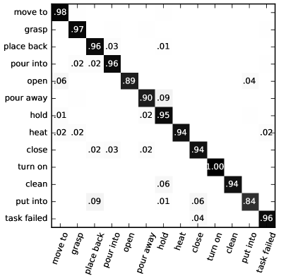
Figure 7: The confusion matrices of the (a) primitive actions and (b) associated objects. Our method can accurately predict both the primitive actions and associated objects.

VI-D Comparisons with the baseline models

We first evaluate the performance of our model for recognizing the primitive actions and associated objects. Figure 7 presents the confusion matrices for these two elements, where our model achieves very high accuracies for most classes. Table I further depicts the detailed comparison of our model against the baseline methods. Our model can predict the primitive actions and associated objects with overall accuracies of 96.1% and 96.6%, outperforming the baseline methods. We also present the mean accuracy of the atomic action in Table II. Here, we compute the accuracy of each atomic action and compute the mean over the accuracies of all the atomic actions. As shown, our model also achieves the highest accuracy compared with the baseline methods.

Then, we evaluate the sequence accuracy of all the methods, as reported in Table III. Our model can correctly predict complete action sequences with an overall probability of 93.7%, evidently outperforming the baseline methods on most tasks (11/12) and improves the overall accuracy by 8.9%.

Some atomic action sequences generated by our method are presented in Figure 8. As shown, our method is capable of accurately predicting the action sequences for various tasks across different scenarios.

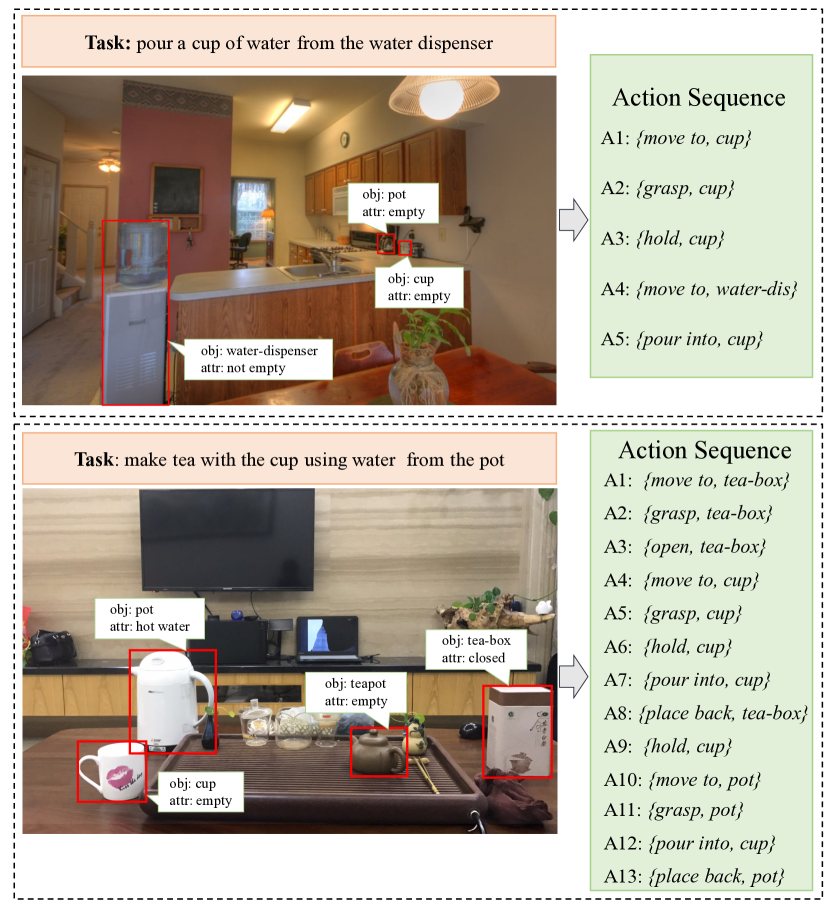
Figure 8: Some atomic action sequences regarding given scene images and tasks generated by our method. Our method is able to correctly predict the action sequence for various tasks across different scenarios.

VI-E Generalization to related tasks

Here, we define “related tasks” as tasks that have similar atomic actions or temporal context to the existing tasks in the training set. For example, “pour a cup of water from the water dispenser” is a task related to “pour a cup of water ”. Thus, it would be interesting to see how our trained model can be generalized to related tasks. In particular, for each related task, we have its AOG representation but no annotated training samples. In this experiment, the models of “Ours without AOG” are all trained on the training set, which only contains samples of task 1 to task 12, as described above. For our model with AOG, we first train the AOG-LSTM with the same set of annotated samples as the other competing models. Subsequently, we utilize the trained AOG-LSTM to produce samples for all tasks, including tasks 13, 14 and 15, and then, we use these samples to train the Action-LSTM. The results of the three tasks are presented in Table IV. We find that the performances of the method without using AOG are extremely unsatisfying on both tasks. These results clearly demonstrate the excellent generalization ability of our model, which improves the sequence accuracy by 63.2%. We also present the sequence accuracy of the AOG-LSTM, i.e., 82.8%, which is also worse than the proposed model.

methods	task 13	task 14	task 15	overall
Ours w/ self aug	6.2	84.6	84.6	70.0
Ours w/o AOG	0.0	26.9	30.8	22.1
Ours w/ AOG	62.5	92.3	92.3	85.3

TABLE IV: Sequence accuracy of our model with and without and-or graph (Ours w/ and w/o AOG) and the Ours w/ self aug. Tasks 13, 14 and 15 denote the “make tea with the cup using water from the pot”, “get a cup of hot water from the water dispenser”, and “pour a cup of water from the water dispenser” tasks, respectively.

VI-F Ablation Study

In this subsection, we perform ablative studies to carefully analyze the contributions of the critical components of our proposed model.

VI-F1 Benefit of using and-or graph

In this experiment, we empirically evaluate the contribution of introducing AOG to the neural network learning. Here, we train the Action-LSTM with and without using the augmented sample set, and we report the results in the last two rows of Table I and Table III, i.e., Ours w/ and w/o AOG. It can be observed that the results using AOGs show a notable improvement in both atomic action recognition and sequence prediction. The performance improvements clearly demonstrate the effectiveness of adopting the augmented set. In particular, generating samples from AOG representations enables us to better capture the complex task variations and is an effective way of compensating the neural network learning. Moreover, note that the Action-LSTM network performs better than the traditional RNN model because LSTM is better able to memorize long-term dependencies among actions.

As discussed above, the trained Action-LSTM can also generate pseudo-labels for unseen samples, and it does not require manually defined AOGs. To see whether the AOGs actually improve the performance, we further implement another baseline (namely, Ours w/ self aug) that uses the Action-LSTM trained on the annotated set to automatically generate a large number of training samples, and then, we train another Action-LSTM using both the annotated and automatically augmented sets. As shown in Table III, this achieves an overall sequence accuracy of 91.5%, better than the baseline Action-LSTM but much worse than our network, i.e., 93.7%. In addition, when generalizing to unseen tasks, our method has an even more notable improvement over this baseline, i.e., 85.3% by ours and 70% by this baseline as shown in Table IV.

VI-F2 Analysis of AOG-LSTM

The AOG-LSTM can also generate action sequences by collecting the leaf nodes after all the or-nodes have been selected. Here, we analyze the performance of the AOG-LSTM network. As shown in Table V, if both are trained only with the annotated set, the Action-LSTM network performs worse than the AOG-LSTM network. This is because making a selection at the or-nodes is less ambiguous because the AOG representation effectively regularizes the semantic space. Thus, the AOG-LSTM network can achieve a reasonable performance despite being trained using a small number of samples. However, when trained with both the annotated and augmented sets, the Action-LSTM network, in turn, outperforms the AOG-LSTM network. One possible reason is as follows. If giving sufficient training samples, the Action-LSTM network may implicitly learn the semantic structures of the And-Or Graph. Moreover, the Action-LSTM model directly predicts the atomic action, and thus, the predicted atomic action in the previous step may provide strong guidance for the subsequent atomic action prediction. However, the or-node prediction of the AOG-LSTM may not have such a property. Moreover, the Action-LSTM is a more flexible and general framework, and it can also achieve reasonable results without the AOG representation (see Ours w/ AOG). Introducing AOG augmentation can further boost its performance, especially for unseen tasks (see Table IV).

Some samples of or-node selection and the corresponding atomic sequences are presented in Figure 9. We find that, for most cases, the AOG-LSTM network can predict the or-node selections correctly, but it is possible to make incorrect predictions if the objects in the image are too complex.

Methods	Sequence acc.
AOG-LSTM w/o aug	91.8
AOG-LSTM w/ aug	92.4
Action-LSTM w/o aug	88.1
Action-LSTM w/ aug	93.7

TABLE V: Sequence accuracy of the AOG-LSTM network trained with and without augmented set and Action-LSTM trained with and without augmented set.

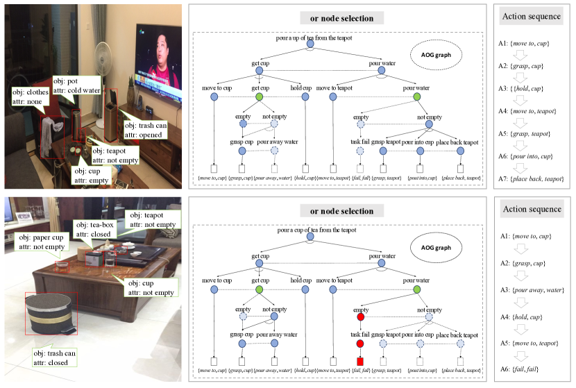
Figure 9: Some samples of or-node selection and the corresponding atomic sequences. The nodes of the unselected branch are denoted as circles with dotted line, and the nodes of incorrectly selected branch are denoted as circles filled with red.

VI-F3 Benefit of curriculum learning

In this part, we perform an experiment to analyze the contribution of employing the curriculum learning algorithm. Here, we train the Action-LSTM network directly using the entire augmented sample set, and we compare it with our network trained using curriculum learning. The results are reported in Table VI. As shown, training the network using curriculum learning clearly improves the performance on both atomic action recognition and sequence prediction. This comparison clearly demonstrates the benefit of applying curriculum learning. Concretely, starting the training of the network using the most reliable samples can effectively avoid disturbances incurred by the difficult samples with uncertain or even incorrect labels and thus produce a network with better initialization performance. In this way, we can better utilize the augmented sample set to train the Action-LSTM network.

Methods	Sequence acc.
Ours w/o CL	92.9
Ours w/ CL	93.7

TABLE VI: Sequence accuracy of by our model with and without the curriculum learning (CL) algorithm. Here, we report the sequence accuracy averaged over task 1 to task 12.

VI-F4 Benefit of predicting the primitive action and associated object independently

To address the problem whereby few samples exist for many atomic actions, we simplify the network by assuming the independence of primitive actions and associated objects, and we predict them separately. Here, we conduct an experiment to evaluate the benefit of this simplification. Because there are 35 atomic actions in total, we first remove the two softmax layers in the Action-LSTM network and employ a 35-class softmax layer to directly predict the atomic action, with the other layers left unchanged. We present the sequence accuracy results in Table VII. Predicting the primitive action and associated object independently can achieve higher sequence accuracies. In particular, this simplification is beneficial for avoiding learning from very few samples and thus enables learning a more robust network.

As discussed in Section V, predicting the primitive action and associated object separately depends on the independence assumption between these two factors. To verify the reasonability of this simplification, we also design some variants that predict the action first and, conditioned on it, predict the object. More concretely, we implement two variants: 1) Action-LSTM with object condition shares the same architecture with the proposed Action-LSTM network except that, at each step, it first predict the score vector of the action and then concatenates it with the hidden state of this step to predict the score vector of the object. 2) Stacked LSTM with object condition employs two stack LSTM networks, in which the first network predicts the score vector of the action, and then, the score vector together with the hidden state is fed to the second network to predict the score vector of the object. For a fair comparison, we set the dimension of the hidden state as 512 and train the two variants in an identical manner. As shown in Table VII, the two variants perform slightly worse than the proposed methods. One possible reason for this may be that the prediction of the object also depends on the predicted action, and these dependencies are also rare in the training set. These comparisons show that this simplification can simplify the network while also improving performance.

Methods	Sequence acc.
Action-LSTM (joint)	91.3
Action-LSTM (condition)	92.3
Stacked LSTM (condition)	92.6
Action-LSTM	93.7

TABLE VII: Sequence accuracy of Action-LSTM predicting primitive action and associated object separately (Action-LSTM), directly predicting the atomic action (Action-LSTM (joint)), Action-LSTM with object condition (Action-LSTM (condition)) and Stacked LSTM with object condition (Stacked LSTM (condition)). Here, we report the sequence accuracy averaged over task 1 to task 12.

VI-F5 Evaluation of task embedding

In this work, we use the one-hot vector for task encoding because there are only 15 tasks, and this simple method can well represent each task. To compare this method with other embedding methods, we also conduct an experiment that utilizes semantic embedding for the tasks. Concretely, we use the trained GloVe model [75] to encode a semantic vector for each word of a specific task and average the vectors of all words to achieve the representation of this task. We use this representation to replace the one-hot encoding and re-train the AOG-LSTM and Action-LSTM. We find that the overall sequence accuracy drops from 93.7% to 92.3%, as shown in Table VIII. One possible reason for this may be as follows. There are only 15 tasks; simple one-hot encoding can well represent each task. If using the more complex semantic representation, by learning from merely 15 sentences, it may be difficult to capture the differences among different tasks.

Methods	Sequence acc.
Ours (GloVe)	92.3
Ours (one-hot)	93.7

TABLE VIII: Sequence accuracy of our method using Glove and one-hot encoding for task embedding. Here, we report the sequence accuracy averaged over task 1 to task 12.

VI-G Results for noisy environments

The above-mentioned experiments are conducted under the assumption of perfect object/attribute detection. It is more practical to evaluate the method in noisy environments. To this end, we further conduct an experiment on noise settings. Specifically, we add Gaussian noise to the one-hot vector of the class label and those of the attributes, and thus, the one-hot vector becomes the score vector, with each element denoting the confidence of the corresponding category or state. We regard the score vector as positive if the bit corresponding to the ground-truth labels has the largest value; otherwise, it is regarded as negative. We add different levels of noise to obtain different negative ratios (e.g., 10% and 20%) in both the training and test set, and we re-train the Action-LSTM network. As shown in Table IX, our network with negative ratios of 10% and 20% error labels achieves sequence accuracies of 46.2% and 41.2%, respectively.

To better evaluate the performance in a real vision system, we further train a Faster R-CNN detector [14] on the training set to automatically detect objects in the given image. We still train the AOG-LSTM and Action-LSTM networks using the annotated objects and evaluate on the test set using the objects detected by the detector. As shown in Table IX, our network can also achieve reasonable results, e.g., an overall sequence accuracy of 55.0%.

Methods	Sequence acc.
Ours w/ 10% noise	46.6
Ours w/ 20% noise	41.2
Ours using detector	55.0
Ours w/o noise	93.7

TABLE IX: Sequence accuracy of our model under the setting of perfect detection, 10%noise and 20% noise (Ours w/o noise, Ours w/ 10% noise, and Ours w/ 20% noise), and automatic detection (Ours using detector). Here, we report the sequence accuracy averaged over task 1 to task 12, where the networks are only trained with the manually annotated set.

VII Conclusion

In this paper, we address a challenging problem, i.e., predicting a sequence of actions to accomplish a specific task under a certain scene, by developing a recurrent LSTM network. To alleviate the issue of requiring large amounts of annotated data, we present a two-stage model training approach by employing a knowledge AOG representation. From this representation, we can produce a large number of valid samples (i.e., task-oriented action sequences) that facilitate learning of the LSTM network. Extensive experiments on a newly created dataset demonstrate the effectiveness and flexibility of our approach.

This is an early attempt to address the task of semantic task planning, but there are certain limitations that prevent the proposed method from extending to more realistic setups. First, the images are pre-processed into a handcrafted feature vector that contains information about the object categories and locations. This pre-processing prevents the model from using end-to-end training and being robust to inference, and these low-dimensional features can only capture limited characteristics of the visual scene. Second, the model was only evaluated on still images; it is unclear if it can easily be extended to a real robot to perform tasks. Third, the structure of the AOG is manually defined; this can be expensive to collect and is a less flexible option. In future work, we will resort to simulation platforms such as AI2-THOR [76, 77] to collect large numbers of annotated samples to train the detectors and classifiers. In this way, we can extricate the model from dependencies on handcrafted image pre-processing, automatically detect objects in a scene and predict their initial states of the attributes. Moreover, we can also enable an agent to interact with objects and perform tasks on these platforms to evaluate our model. On the other hand, we will also explore automatically learning the AOG structure from annotated samples, thereby improving the flexibility and extendibility of the proposed method.

Tianshui Chen received his B.E. degree from the School of Information and Science Technology, Sun Yat-sen University, Guangzhou, China, in 2013. He is currently pursuing his Ph.D. degree in computer science with the School of Data and Computer Science. His current research interests include computer vision and machine learning. He was the recipient of Best Paper Diamond Award in IEEE ICME 2017.

Riquan Chen received his B.E. degree from the School of Mathematics, Sun Yat-sen University, Guangzhou, China, in 2017, where he is currently pursuing his Master’s Degree in computer science with the School of Data and Computer Science. His current research interests include computer vision and machine learning.

Lin Nie is an Assistant Researcher with the Center for Shared Experimental Education, Sun Yat-Sen University (SYSU), China. She received her B.S. degree from the Beijing Institute of Technology (BIT), China in 2004 and her M.S. degree from the Department of Statistics, University of California, Los Angeles (UCLA). Her research focuses on data mining and pattern recognition.

Xiaonan Luo was the Director of the National Engineering Research Center of Digital Life, Sun Yat-sen University, Guangzhou, China. He is currently a Professor with the School of Computer Science and Information Security, Guilin University of Electronic Technology, Guilin, China. He received the National Science Fund for Distinguished Young Scholars granted by the National Nature Science Foundation of China. His research interests include computer graphics, CAD, image processing, and mobile computing.

Xiaobai Liu is an Assistant Professor of Computer Science at San Diego State University (SDSU), San Diego, U.S.A. He received his PhD from the Huazhong University of Science and Technology (HUST), China. His research interests focus on the development of theories, algorithms, and models for core computer vision problems, including image parsing, 3D vision, and visual tracking. He has published 50 peer-reviewed articles in top-tier conferences (e.g.,ICCV and CVPR) and leading journals (e.g., TPAMI and TIP). He received a number of awards for his academic contributions, including the outstanding thesis award by CCF (China Computer Federation).

Liang Lin (M’09, SM’15) is the Executive Research Director of SenseTime Group Limited and a full Professor of Sun Yat-sen University. He is the Excellent Young Scientist of the National Natural Science Foundation of China. From 2008 to 2010, he was a Post-Doctoral Fellow at University of California, Los Angeles. From 2014 to 2015, as a senior visiting scholar, he was with The Hong Kong Polytechnic University and The Chinese University of Hong Kong. He currently leads the SenseTime R&D teams in developing cutting-edge and deliverable solutions on computer vision, data analysis and mining, and intelligent robotic systems. He has authored and co-authored more than 100 papers in top-tier academic journals and conferences (e.g., 10 papers in TPAMI/IJCV and 40+ papers in CVPR/ICCV/NIPS/IJCAI). He has been serving as an associate editor of IEEE Trans. Human-Machine Systems, The Visual Computer and Neurocomputing. He served as Area/Session Chair for numerous conferences such as ICME, ACCV, and ICMR. He was the recipient of Best Paper Runner-Up Award in ACM NPAR 2010, the Google Faculty Award in 2012, the Best Paper Diamond Award at IEEE ICME 2017, and Hong Kong Scholars Award in 2014. He is a Fellow of IET.

References

- [1] S. Thrun, W. Burgard, and D. Fox, Probabilistic robotics. MIT press, 2005.
- [2] L. E. Parker, “L-alliance: Task-oriented multi-robot learning in behavior-based systems,” Advanced Robotics, vol. 11, no. 4, pp. 305–322, 1996.
- [3] A. Krizhevsky, I. Sutskever, and G. E. Hinton, “Imagenet classification with deep convolutional neural networks,” in Advances in neural information processing systems, 2012, pp. 1097–1105.
- [4] M. D. Zeiler and R. Fergus, “Visualizing and understanding convolutional networks,” in Proceedings of European conference on computer vision. Springer, 2014, pp. 818–833.
- [5] K. Simonyan and A. Zisserman, “Very deep convolutional networks for large-scale image recognition,” arXiv preprint arXiv:1409.1556, 2014.
- [6] K. He, X. Zhang, S. Ren, and J. Sun, “Deep residual learning for image recognition,” in Proceedings of the IEEE conference on computer vision and pattern recognition, 2016, pp. 770–778.
- [7] A. Wang, J. Lu, J. Cai, T.-J. Cham, and G. Wang, “Large-margin multi-modal deep learning for rgb-d object recognition,” IEEE Transactions on Multimedia, vol. 17, no. 11, pp. 1887–1898, 2015.
- [8] A. H. Abdulnabi, G. Wang, J. Lu, and K. Jia, “Multi-task cnn model for attribute prediction,” IEEE Transactions on Multimedia, vol. 17, no. 11, pp. 1949–1959, 2015.
- [9] B. Zhao, X. Wu, J. Feng, Q. Peng, and S. Yan, “Diversified visual attention networks for fine-grained object classification,” IEEE Transactions on Multimedia, vol. 19, no. 6, pp. 1245–1256, 2017.
- [10] T. Chen, Z. Wang, G. Li, and L. Lin, “Recurrent attentional reinforcement learning for multi-label image recognition,” in Proc. of AAAI Conference on Artificial Intelligence, 2018, pp. 6730–6737.
- [11] Z. Wang, T. Chen, G. Li, R. Xu, and L. Lin, “Multi-label image recognition by recurrently discovering attentional regions,” in Proceedings of the IEEE international conference on computer vision, 2017.
- [12] T. Chen, L. Lin, R. Chen, Y. Wu, and X. Luo, “Knowledge-embedded representation learning for fine-grained image recognition,” in Proc. of International Joint Conference on Artificial Intelligence, 2018, pp. 627–634.
- [13] T. Chen, W. Wu, Y. Gao, L. Dong, X. Luo, and L. Lin, “Fine-grained representation learning and recognition by exploiting hierarchical semantic embedding,” in Proc. of ACM International Conference on Multimedia, 2018.
- [14] S. Ren, K. He, R. Girshick, and J. Sun, “Faster r-cnn: Towards real-time object detection with region proposal networks,” in Advances in neural information processing systems, 2015, pp. 91–99.
- [15] J. Li, Y. Wei, X. Liang, J. Dong, T. Xu, J. Feng, and S. Yan, “Attentive contexts for object detection,” IEEE Transactions on Multimedia, vol. 19, no. 5, pp. 944–954, 2017.
- [16] T. Chen, L. Lin, X. Wu, N. Xiao, and X. Luo, “Learning to segment object candidates via recursive neural networks,” IEEE Transactions on Image Processing, 2018.
- [17] T. Chen, L. Lin, L. Liu, X. Luo, and X. Li, “Disc: Deep image saliency computing via progressive representation learning.” IEEE Trans. Neural Netw. Learning Syst., vol. 27, no. 6, pp. 1135–1149, 2016.
- [18] S. Hochreiter and J. Schmidhuber, “Long short-term memory,” Neural computation, vol. 9, no. 8, pp. 1735–1780, 1997.
- [19] K. Cho, B. Van Merriënboer, C. Gulcehre, D. Bahdanau, F. Bougares, H. Schwenk, and Y. Bengio, “Learning phrase representations using rnn encoder-decoder for statistical machine translation,” in Proceeding of Empirical Methods in Natural Language Processing, 2014.
- [20] O. Vinyals, A. Toshev, S. Bengio, and D. Erhan, “Show and tell: A neural image caption generator,” in Proceedings of the IEEE conference on computer vision and pattern recognition, 2015, pp. 3156–3164.
- [21] L. Gao, Z. Guo, H. Zhang, X. Xu, and H. T. Shen, “Video captioning with attention-based lstm and semantic consistency,” IEEE Transactions on Multimedia, vol. 19, no. 9, pp. 2045–2055, 2017.
- [22] L. Lin, H. Gong, L. Li, and L. Wang, “Semantic event representation and recognition using syntactic attribute graph grammar,” Pattern Recognition Letters, vol. 30, no. 2, pp. 180–186, 2009.
- [23] C. Xiong, N. Shukla, W. Xiong, and S.-C. Zhu, “Robot learning with a spatial, temporal, and causal and-or graph,” Proceedings of the IEEE International Conference on Robotics and Automation, 2016.
- [24] W. Li, J. Joo, H. Qi, and S.-C. Zhu, “Joint image-text news topic detection and tracking by multimodal topic and-or graph,” IEEE Transactions on Multimedia, vol. 19, no. 2, pp. 367–381, 2017.
- [25] L. Lin, L. Huang, T. Chen, Y. Gan, and H. Chen, “Knowledge-guided recurrent neural network learning for task-oriented action prediction,” in Proceedings of IEEE International Conference on Multimedia & Expo, 2017.
- [26] Y. Bengio, J. Louradour, R. Collobert, and J. Weston, “Curriculum learning,” in Proceedings of the 26th annual international conference on machine learning. ACM, 2009, pp. 41–48.
- [27] F. Khan, B. Mutlu, and X. Zhu, “How do humans teach: On curriculum learning and teaching dimension,” in Advances in Neural Information Processing Systems, 2011, pp. 1449–1457.
- [28] J. Sung, B. Selman, and A. Saxena, “Learning sequences of controllers for complex manipulation tasks,” in Proceedings of the International Conference on Machine Learning, 2013.
- [29] J. F. Allen, “Planning as temporal reasoning.” in Principles of Knowledge Representation and Reasoning, vol. 91, 1991, pp. 3–14.
- [30] D. E. Smith and D. S. Weld, “Temporal planning with mutual exclusion reasoning,” in Proceedings of the International Joint Conference on Artificial Intelligence, vol. 99, 1999, pp. 326–337.
- [31] H. A. Kautz, B. Selman et al., “Planning as satisfiability.” in Proceedings of the European Conference on Artificial Intelligence, vol. 92, 1992, pp. 359–363.
- [32] J. Rintanen, K. Heljanko, and I. Niemelä, “Planning as satisfiability: parallel plans and algorithms for plan search,” Artificial Intelligence, vol. 170, no. 12-13, pp. 1031–1080, 2006.
- [33] E. D. Sacerdoti, “Planning in a hierarchy of abstraction spaces,” Artificial intelligence, vol. 5, no. 2, pp. 115–135, 1974.
- [34] Q. Yang, K. Wu, and Y. Jiang, “Learning action models from plan examples using weighted max-sat,” Artificial Intelligence, vol. 171, no. 2, pp. 107–143, 2007.
- [35] S. Kambhampati, M. R. Cutkosky, M. Tenenbaum, and S. Lee, “Combining specialized reasoners and general purpose planners: A case study.” in Proceedings of the Association for the Advancement of Artificial Intelligence, 1991, pp. 199–205.
- [36] S. Cambon, R. Alami, and F. Gravot, “A hybrid approach to intricate motion, manipulation and task planning,” The International Journal of Robotics Research, vol. 28, no. 1, pp. 104–126, 2009.
- [37] E. Plaku and G. Hager, “Sampling-based motion and symbolic action planning with geometric and differential constraints,” in Proceedings of the IEEE International Conference on Robotics and Automation, 2010, pp. 5002–5008.
- [38] J. Wolfe, B. Marthi, and S. Russell, “Combined task and motion planning for mobile manipulation.” in Proceedings of the International Conference on Automated Planning and Scheduling, 2010, pp. 254–258.
- [39] J. Sung, B. Selman, and A. Saxena, “Synthesizing manipulation sequences for under-specified tasks using unrolled markov random fields,” in Proceedings of the IEEE/RSJ International Conference on Intelligent Robots and Systems. IEEE, 2014, pp. 2970–2977.
- [40] S. Z. Li, “Markov random field models in computer vision,” in Proceedings of the European conference on computer vision. Springer, 1994, pp. 361–370.
- [41] M. Bollini, J. Barry, and D. Rus, “Bakebot: Baking cookies with the pr2,” in The PR2 workshop: results, challenges and lessons learned in advancing robots with a common platform, IROS, 2011.
- [42] M. Beetz, U. Klank, I. Kresse, A. Maldonado, L. Mösenlechner, D. Pangercic, T. Rühr, and M. Tenorth, “Robotic roommates making pancakes,” in Proceedings of the IEEE-RAS International Conference on Humanoid Robots (Humanoids). IEEE, 2011, pp. 529–536.
- [43] S. Miller, J. Van Den Berg, M. Fritz, T. Darrell, K. Goldberg, and P. Abbeel, “A geometric approach to robotic laundry folding,” The International Journal of Robotics Research, vol. 31, no. 2, pp. 249–267, 2012.
- [44] Y. Zhu, D. Gordon, E. Kolve, D. Fox, L. Fei-Fei, A. Gupta, R. Mottaghi, and A. Farhadi, “Visual semantic planning using deep successor representations,” in Proceedings of the IEEE International Conference on Computer Vision, vol. 2, no. 4, 2017, p. 7.
- [45] S. Gupta, J. Davidson, S. Levine, R. Sukthankar, and J. Malik, “Cognitive mapping and planning for visual navigation,” in Proceedings of the IEEE Conference on Computer Vision and Pattern Recognition, 2017, pp. 2616–2625.
- [46] R. Pascanu, Y. Li, O. Vinyals, N. Heess, L. Buesing, S. Racanière, D. Reichert, T. Weber, D. Wierstra, and P. Battaglia, “Learning model-based planning from scratch,” arXiv preprint arXiv:1707.06170, 2017.
- [47] P. Agrawal, A. V. Nair, P. Abbeel, J. Malik, and S. Levine, “Learning to poke by poking: Experiential learning of intuitive physics,” in Advances in Neural Information Processing Systems, 2016, pp. 5074–5082.
- [48] C. Finn and S. Levine, “Deep visual foresight for planning robot motion,” in Robotics and Automation (ICRA), 2017 IEEE International Conference on. IEEE, 2017, pp. 2786–2793.
- [49] B. Wu, C. Yuan, and W. Hu, “Human action recognition based on context-dependent graph kernels,” in Proceedings of the IEEE Conference on Computer Vision and Pattern Recognition, 2014, pp. 2609–2616.
- [50] W. Xu, Z. Miao, X.-P. Zhang, and Y. Tian, “A hierarchical spatio-temporal model for human activity recognition,” IEEE Transactions on Multimedia, vol. 19, no. 7, pp. 1494–1509, 2017.
- [51] S. Samanta and B. Chanda, “Space-time facet model for human activity classification,” IEEE Transactions on Multimedia, vol. 16, no. 6, pp. 1525–1535, 2014.
- [52] Y. Guo, D. Tao, J. Cheng, A. Dougherty, Y. Li, K. Yue, and B. Zhang, “Tensor manifold discriminant projections for acceleration-based human activity recognition,” IEEE Transactions on Multimedia, vol. 18, no. 10, pp. 1977–1987, 2016.
- [53] L. Lin, K. Wang, W. Zuo, M. Wang, J. Luo, and L. Zhang, “A deep structured model with radius–margin bound for 3d human activity recognition,” International Journal of Computer Vision, vol. 118, no. 2, pp. 256–273, 2016.
- [54] Y. Kong, D. Kit, and Y. Fu, “A discriminative model with multiple temporal scales for action prediction,” in Proceedings of the European Conference on Computer Vision. Springer, 2014, pp. 596–611.
- [55] T. Lan, T.-C. Chen, and S. Savarese, “A hierarchical representation for future action prediction,” in Proceedings of the European Conference on Computer Vision. Springer, 2014, pp. 689–704.
- [56] L. Wang, X. Zhao, Y. Si, L. Cao, and Y. Liu, “Context-associative hierarchical memory model for human activity recognition and prediction,” IEEE Transactions on Multimedia, vol. 19, no. 3, pp. 646–659, 2017.
- [57] J. T. Connor, R. D. Martin, and L. E. Atlas, “Recurrent neural networks and robust time series prediction,” IEEE transactions on neural networks, vol. 5, no. 2, pp. 240–254, 1994.
- [58] T.-h. Wen, P.-h. Su, V. David, and S. Young, “Semantically conditioned lstm-based natural language generation for spoken dialogue systems,” in In Proceedings of EMNLP. Association for Computational Linguistics. Citeseer, 2015.
- [59] A. Rush, S. Chopra, and J. Weston, “A neural attention model for abstractive sentence summarization,” arXiv preprint arXiv:1509.00685, 2015.
- [60] J. Tang, Y. Yang, S. Carton, M. Zhang, and Q. Mei, “Context-aware natural language generation with recurrent neural networks,” arXiv preprint arXiv:1611.09900, 2016.
- [61] D. Bahdanau, K. Cho, and Y. Bengio, “Neural machine translation by jointly learning to align and translate,” arXiv preprint arXiv:1409.0473, 2014.
- [62] K. Cho, B. Van Merriënboer, D. Bahdanau, and Y. Bengio, “On the properties of neural machine translation: Encoder-decoder approaches,” arXiv preprint arXiv:1409.1259, 2014.
- [63] Y. Wu, M. Schuster, Z. Chen, Q. V. Le, M. Norouzi, W. Macherey, M. Krikun, Y. Cao, Q. Gao, K. Macherey et al., “Google’s neural machine translation system: Bridging the gap between human and machine translation,” arXiv preprint arXiv:1609.08144, 2016.
- [64] L. Yao, A. Torabi, K. Cho, N. Ballas, C. Pal, H. Larochelle, and A. Courville, “Describing videos by exploiting temporal structure,” in Proceedings of the IEEE international conference on computer vision, 2015, pp. 4507–4515.
- [65] Q. You, H. Jin, Z. Wang, C. Fang, and J. Luo, “Image captioning with semantic attention,” in Proceedings of the IEEE Conference on Computer Vision and Pattern Recognition, 2016, pp. 4651–4659.
- [66] P. Pan, Z. Xu, Y. Yang, F. Wu, and Y. Zhuang, “Hierarchical recurrent neural encoder for video representation with application to captioning,” in Proceedings of the IEEE Conference on Computer Vision and Pattern Recognition, 2016, pp. 1029–1038.
- [67] F. Harary, “The determinant of the adjacency matrix of a graph,” Siam Review, vol. 4, no. 3, pp. 202–210, 1962.
- [68] V. Nair and G. E. Hinton, “Rectified linear units improve restricted boltzmann machines,” in Proceedings of the 27th international conference on machine learning, 2010, pp. 807–814.
- [69] Y. Zhu, A. Fathi, and L. Fei-Fei, “Reasoning about object affordances in a knowledge base representation,” in European conference on computer vision. Springer, 2014, pp. 408–424.
- [70] I. Białynicki-Birula and J. Mycielski, “Uncertainty relations for information entropy in wave mechanics,” Communications in Mathematical Physics, vol. 44, no. 2, pp. 129–132, 1975.
- [71] E. T. Jaynes, “Information theory and statistical mechanics,” Physical review, vol. 106, no. 4, p. 620, 1957.
- [72] Y. Jia, E. Shelhamer, J. Donahue, S. Karayev, J. Long, R. Girshick, S. Guadarrama, and T. Darrell, “Caffe: Convolutional architecture for fast feature embedding,” in ACM Multimedia, 2014, pp. 675–678.
- [73] L. Bottou, “Large-scale machine learning with stochastic gradient descent,” in Proceedings of COMPSTAT’2010. Springer, 2010, pp. 177–186.
- [74] M. W. Gardner and S. Dorling, “Artificial neural networks (the multilayer perceptron) - a review of applications in the atmospheric sciences,” Atmospheric environment, vol. 32, no. 14, pp. 2627–2636, 1998.
- [75] J. Pennington, R. Socher, and C. Manning, “Glove: Global vectors for word representation,” in Proceedings of the conference on empirical methods in natural language processing (EMNLP), 2014, pp. 1532–1543.
- [76] Y. Zhu, R. Mottaghi, E. Kolve, J. J. Lim, A. Gupta, L. Fei-Fei, and A. Farhadi, “Target-driven visual navigation in indoor scenes using deep reinforcement learning,” in Robotics and Automation (ICRA), 2017 IEEE International Conference on. IEEE, 2017, pp. 3357–3364.
- [77] E. Kolve, R. Mottaghi, D. Gordon, Y. Zhu, A. Gupta, and A. Farhadi, “Ai2-thor: An interactive 3d environment for visual ai,” arXiv preprint arXiv:1712.05474, 2017.