Nuclear structure studies of double Gamow-Teller strength

Abstract

The double Gamow-Teller strength distributions in even-$A$ Calcium isotopes were calculated using the nuclear shell model by applying the single Gamow-Teller operator two times sequentially on the ground state of the parent nucleus. The number of intermediate states actually contributing to the results was determined. The sum rules for the double Gamow-Teller operator in the full calculation were approximately fulfilled. In the case that the symmetry is restored approximately by introducing degeneracies of the $f$-levels, and the $p$-levels in the $fp$-model space, the agreement with the sum rules was very close.

I Introduction

The double charge-exchange (DCX) processes are a promising tool to study nuclear structure in particular nucleon-nucleon correlations in nuclei. In the 1980s, the DCX reactions using pion beams that were produced in the three meson factories at LAMPF, TRIUMF, and SIN were performed. Studies at lower pion energies ($E\leq 50$ MeV) have indeed produced clear signals of nucleon-nucleon correlations PhysRevLett.52.105 ; PhysRevLett.54.1482 ; PhysRevC.35.1425 ; PhysRevC.37.902 ; WEINFELD199033 and were successfully explained by the theoretical studies PhysRevLett.59.1076 ; PhysRevC.38.1277 . The pion DCX experiments discovered the double isobaric analog states (DIAS) PhysRevC.35.1334 ; PhysRevC.36.1479 . At higher pion energies ($E>300$ MeV), the studies discovered the giant dipole resonances (GDR) built on the IAS PhysRevLett.60.408 ; PhysRevC.38.2709 ; PhysRevC.40.850 ; PhysRevC.43.1111 , and double giant dipole resonances (DGDR) PhysRevLett.61.531 ; PhysRevC.41.202 ; PhysRevC.43.1318 ; PhysRevC.43.R1509 (See Refs. PhysRevLett.60.408 ; PhysRevLett.61.531 for definitions).

At present, there is a renewed interest in DCX reactions, to a large extent due to the extensive studies of double beta-decay, both the decay in which two neutrinos are emitted ($2\nu\beta\beta$) and neutrinoless double beta ($0\nu\beta\beta$) decay. In DCX and $\beta\beta$ decay, two nucleons are involved. The pion, however, interacts weakly with states involving the spin and the pion DCX reactions do not excite the states involving the spin, such as the double Gamow-Teller (DGT) state. The DGT strength is the essential part of the $\beta\beta$ decay transitions. It was suggested in the past that one could probe the DGT state and hopefully the $0\nu\beta\beta$ decay using DCX reactions with light ions ZHENG1990343 ; Cappuzzello2015 .

In present days, DCX reactions are performed using light ions. There is a large program called NUMEN in Catania where reactions with ¹⁸O, and ¹⁸Ne have been done Cappuzzello2018 . The hope is that such studies might shed some light on the nature of the nuclear matrix element of the double beta-decay and serve as a “calibration” for the size of this matrix element. These DCX studies might also provide new interesting information about nuclear structure. One of the outstanding resonances relevant to the $0\nu\beta\beta$ decay is the double Gamow-Teller (DGT) resonance suggested in the past AUERBACH198977 ; ZHENG1990343 . At RIKEN, there is a DCX program using ion beams for the purpose of observing DGT states and other nuclear structure studies UesakaCommu . At Osaka University, the new DCX reactions with light ions were used to excite the double charge exchange state and compare to the pion DCX reaction results. One additional peak appeared in the cross-section suggesting that it is a DGT resonance Ejiri2017 .

The DGT strength distributions in even-$A$ Neon isotopes was discussed in Ref. MUTO199213 and recently the calculation of DGT strength for ⁴⁸Ca was performed in Ref. PhysRevLett.120.142502 . In the present paper, the DGT transition strength distributions in even-$A$ Calcium isotopes are calculated in the full $fp$-model space using the nuclear shell model code NuShellX@MSU BROWN2014115 ; BROWN2001517 . The single Gamow-Teller operator is applied two times sequentially on the ground state of the parent nucleus to obtain the DGT strength. This method is different from the method used in Refs. MUTO199213 ; PhysRevLett.120.142502 .

The properties of the DGT distribution are examined and limiting cases when the SU(4) holds or when the spin orbit-orbit coupling is put to zero are studied. DGT sum rules were derived in Refs. VOGEL1988259 ; PhysRevC.40.936 ; MUTO199213 , and recently discussed in Ref. PhysRevC.94.064325 . The DGT sum rules were used here as a tool to asses whether in our numerical calculations most of the DGT strength is found.

II Method of calculation

The notion of a DGT was introduced in Refs. AUERBACH198977 ; ZHENG1990343 . First of all, the nuclear shell model wave functions of the initial ground state, $J=1^{+}$ intermediate states, and $J=0^{+},2^{+}$ final states were obtained using the shell model code NuShellX@MSU BROWN2014115 ; BROWN2001517 with the FPD6 RICHTER1991325 and KB3G POVES2001157_KB3G interactions, in the complete $fp$-model space. The maximum of the number of intermediate states is 1000. Table 1 shows the total number of final states that is possible in Ti isotopes. If the total number of final states is larger than 5000, the calculations were done up to 5000 final states. As one will see later, that is enough to exhaust almost the total strength.

Table 1: The total number of final states in the $fp$-model space and $f$-model space including the $f_{7/2}$ and the $f_{5/2}$ orbits only.

	42Ti		44Ti		46Ti		48Ti
$J^{\pi}_{f}$	$0^{+}$	$2^{+}$	$0^{+}$	$2^{+}$	$0^{+}$	$2^{+}$	$0^{+}$	$2^{+}$
$fp$-space	4	8	158	596	2343	9884	14177	61953
$f$-space	2	1	29	99	180	741	446	1899

After all wave functions were obtained, the single GT operator was applied two times sequentially. First, all transitions from the parent nucleus $0^{+}$ to all $1^{+}$ intermediate states are calculated and then all transitions from $1^{+}$ intermediate states to each $0^{+}$ or $2^{+}$ in the final nucleus are calculated. Fig. 1 illustrates the method of calculation.

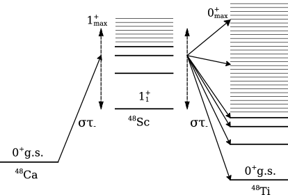
Figure 1: Illustration of the method of calculation described in the text. The notations $1^{+}_{\text{max}}$ and $0^{+}_{\text{max}}$ are the highest states that can be reached in practice.

The single GT operator is denoted as

$$\bm{Y}_{\pm}=\sum_{i=1}^{A}\bm{\sigma}t_{\pm}(i);\quad t_{\pm}=t_{x}\pm it_{y},$$ (1)

with $t_{-}n=p$ and $t_{+}p=n$ where $2t_{x}$ and $2t_{y}$ are the Pauli isospin operators and $\bm{\sigma}$ is Pauli spin operator. Then the single GT transition amplitude from the initial state $|i\rangle$ to the final state $|f\rangle$ is

$$M(GT_{\pm};i\rightarrow f)=\frac{\langle f||\bm{Y}_{\pm}||i\rangle}{\sqrt{2J_{i}+1}},$$ (2)

and the GT transition strength given by

$$B(GT_{\pm})=|M(GT_{\pm};i\rightarrow f)|^{2}$$ (3)

obeys the $"3(N-Z)"$ sum rule:

$$\sum_{f}B(GT_{-})-\sum_{f}B(GT_{+})=S_{GT_{-}}-S_{GT_{+}}=3(N-Z),$$ (4)

where the $\sum_{f}$ means summing over all eigenstates of $J_{f}T_{f}$. Because the $fp$-model space is limited, only the valence neutrons participate in the calculation for Calcium isotopes. Therefore, we have $S_{GT_{+}}=0$.

The dimensionless DGT transition amplitude is defined as

$$M(DGT_{\pm})=\sum_{n}M(GT_{\pm};i\rightarrow n)M(GT_{\pm};n\rightarrow f),$$ (5)

where $n$ are the intermediate states. Note that this is a coherent sum. Finally, the DGT strength is given by

$$B(DGT_{\pm})=|M(DGT_{\pm})|^{2},$$ (6)

or in more detail

$$B(\text{DGT}^{-};i\rightarrow n\rightarrow f)=\frac{1}{2J_{i}+1}\left|\sum_{n}\left\langle f\left|\left|\sum_{i}\bm{\sigma}_{i}t_{-}(i)\right|\right|n\right\rangle\left\langle n\left|\left|\sum_{j}\bm{\sigma}_{j}t_{-}(j)\right|\right|i\right\rangle\right|^{2}.$$ (7)

Note that $B(DGT^{-};i\rightarrow n\rightarrow f)$ depends on $J_{f}$ with $J_{f}=0$ and 2 only. The matrix element in the case $J_{f}=1$ vanishes because the DGT operator changes sign under the interchange of coordinates of two particles.

The DGT sum rule for $J_{f}=0$ is given in Refs. VOGEL1988259 ; PhysRevC.40.936 and $J_{f}=0,2$ are given in Refs. MUTO199213 ; PhysRevC.94.064325 . In summary, the generalization of the sum rules for DGT operators are:

$$S_{\text{DGT}}^{J_{f}=0}=6(N-Z)(N-Z+1)-2\Delta,$$

$$S_{\text{DGT}}^{J_{f}=2}=30(N-Z)(N-Z-2)+5\Delta,$$ (8)

where $\Delta=\sqrt{2}\langle 0|[\bm{Y}_{+}\times\bm{Y}_{-}]^{(1)}\cdot\bm{\varSigma}-\bm{\varSigma}\cdot[\bm{Y}_{-}\times\bm{Y}_{+}]^{(1)}|0\rangle,$ with $\bm{\varSigma}=\sum_{i}\bm{\sigma}(i)$. There is a factor of three difference between our work and the work in Refs. MUTO199213 ; PhysRevLett.120.142502 because the spin operator is not projected in our calculation. The first terms of the sum rules depend only on $N$ and $Z$, and the second terms ($2\Delta$ or $5\Delta$) need to be calculated separately. The sign of the second term makes the first one to be the upper limit for $J_{f}=0^{+}$ and lower limit for $J_{f}=2^{+}$.

III Results and discussions

It is well-known that the single GT strength is quenched (see Ref. RevModPhys.64.491 ). In the shell model calculations, GT strength is fragmented. This is demonstrated in the case of ⁴⁸Ca in Fig. 2 as an example. The results were obtained with two different interactions that are often used in the $fp$-model space FPD6 and KB3G interactions. Within the range of about 17 MeV excitation energy, $S_{GT_{-}}$ is approximately 24 exhausting the $``3(N-Z)"$ sum rule ($S_{GT_{+}}=0$ in our calculation). The cumulative sum of the single GT strength S(GT) as a function of number of ⁴⁸Sc states is shown in Fig. 2. One can expect that there are about 500 intermediate $1^{+}$ states in ⁴⁸Sc that actually contribute to the final results of the DGT strength although the total number of $1^{+}$ states in this nucleus is many thousands.

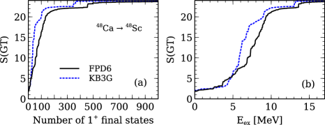
Figure 2: The cumulative sum of the single Gamow-Teller strength B(GT) as a function of the number of $1^{+}$ states (a) and excitation energies (b) of the intermediate nucleus ⁴⁸Sc. The calculation used FPD6 and KB3G interactions in the $fp$-model space.

Table 2: The properties of DGT transition using FPD6 and KB3G interactions in the complete $fp-$model space. $S(\text{DGT})$ is the DGT total strength with the FPD6 interaction. $B_{1}$ is the transition from the g.s. of the parent nucleus to the first $J^{+}$ state of the final nucleus. $\overline{E}$ (MeV) is the average energy (Eq. (9)).

Initial nucleus	42Ca		44Ca		46Ca		48Ca
$J^{\pi}_{f}$	$0^{+}$	$2^{+}$	$0^{+}$	$2^{+}$	$0^{+}$	$2^{+}$	$0^{+}$
$S(\text{DGT})$	1 28.1	1 19.5	102.0	284.0	223.7	752.6	385.0
Sum rule	$\leq 36$	$\geq 0$	$\leq 120$	$\geq 240$	$\leq 252$	$\geq 720$	$\leq 432$
$B_{1}$ (FPD6)	16.172	6.117	0.654	0.000	0.201	0.017	0.109
$B_{1}$ (KB3G)	17.010	5.942	0.895	0.119	0.182	0.057	0.072
$\overline{E}$ (FPD6)	6.1	4.8	16.3	13.2	21.2	18.0	24.6
$\overline{E}$ (KB3G)	6.1	5.5	14.7	12.2	19.0	16.9	21.9

For the study of the DGT, first, we calculated the sum rule using it as a tool to asses whether in our numerical calculations most of the DGT strength is found. The $\Delta$ in Eq. (II) can be obtained directly by subtracting from total sum the first term that depends only on $N$ and $Z$ (see Table 2). In Ref. PhysRevC.40.936 , $\Delta$ was related to the magnetic dipole transition $S(M1)$. Table I in Ref. PhysRevC.40.936 and Table I in Ref. PhysRevC.94.064325 gave the values of the sum rules for even-$A$ isotopes including Calcium isotopes. Our results given in Table 2 are in agreement with them (Note that there is a factor of three difference between our work and Ref. PhysRevC.94.064325 ). It means we exhaust all the DGT strength in the study. Obviously, the total DGT strength does not depend on the choice of interaction.

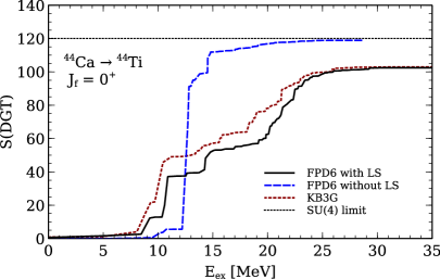
Figure 3: The cumulative sum of the double Gamow-Teller strength $B(\rm{DGT};0^{+}\rightarrow 0^{+})$ in ⁴⁴Ca.

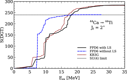
Figure 4: The cumulative sum of the double Gamow-Teller strength $B(\rm{DGT};0^{+}\rightarrow 2^{+})$ in ⁴⁴Ca.

Because all the strengths are obtained, we can show not only the values of the total sum but also the cumulative sums of the DGT. The cumulative sums are given in Fig. 3, and Fig. 4 for ⁴⁴Ca, Fig. 5, and Fig. 6 for ⁴⁶Ca, and Fig. 7 for ⁴⁸Ca. In these figures, the solid lines are the shell model calculations described in Section II using the FPD6 interaction. They are denoted as “FPD6 with LS”. The results using the KB3G interaction are also shown as dotted lines. The long-dash lines are the calculation with the FPD6 interaction in the SU(4) limit. The SU(4) limit in our work is restored approximately by making the $f_{5/2}$ and $f_{7/2}$; $p_{1/2}$ and $p_{3/2}$ degenerate following Ref. PhysRevC.96.044319 . It means there is no spin-orbit coupling and therefore they were denoted as “FPD6 without LS”. We want to show that in the SU(4) limit, the cumulative sums approach the horizontal lines (denoted as the “SU(4) limit”) that represent the values of the terms that depend only on $N$ and $Z$ in Eq. (II). It is in agreement with the fact that $\Delta$ vanishes in the SU(4) limit according to Ref. PhysRevC.39.2370 . In the cases of ⁴⁴Ca (Fig. 3, and Fig. 4), the sum rules are totally exhausted because all intermediate states and all final states can be taken into account. In the cases of ⁴⁶Ca, and ⁴⁸Ca (Figs. 5–7), the cumulative sums are still increasing. For the case of the DGT to the $2^{+}$ in ⁴⁸Ca, we choose not to do the calculation because the total number of final states are too large. The result is not convergent using the standard NUSHELLX@MSU code BrownCommu .

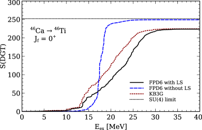
Figure 5: The cumulative sum of the double Gamow-Teller strength $B(\rm{DGT};0^{+}\rightarrow 0^{+})$ in ⁴⁶Ca.

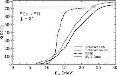
Figure 6: The cumulative sum of the double Gamow-Teller strength $B(\rm{DGT};0^{+}\rightarrow 2^{+})$ in ⁴⁶Ca.

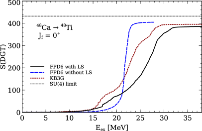
Figure 7: The cumulative sum of the double Gamow-Teller strength $B(\rm{DGT};0^{+}\rightarrow 0^{+})$ in ⁴⁸Ca.

Most of the sum rule is satisfied, and therefore the entire distributions of DGT strength now can be discussed. We remind that Ref. MUTO199213 showed the entire DGT distributions for even-$A$ Neon and recently Ref. PhysRevLett.120.142502 showed the result for ⁴⁸Ca for the first time. For the lightest nucleus, ⁴²Ca, the DGT distributions with FPD6 and KB3G interactions are shown in Table 3 and 4. The difference between the results of the two interactions is not large.

Table 3: $B(\rm{DGT};0^{+}\rightarrow 0^{+})$ for ⁴²Ca using FPD6 and KB3G interactions in the complete $fp$-model space. $E_{ex}$ (MeV) is the excited energy of ⁴²Ti.

	FPD6			KB3G
$E_{ex}$	$B(\rm{DGT})$	$S(\rm{DGT})$	$E_{ex}$	$B(\rm{DGT})$	$S(\rm{DGT})$
0.0	16.172	16.172	0.0	17.010	17.010
6.0	0.442	16.614	5.7	0.281	17.291
10.9	0.782	17.396	11.3	0.120	17.411
14.9	10.692	28.088	15.4	11.085	28.496

Table 4: The same as Table 3, but for $B(\rm{DGT};0^{+}\rightarrow 2^{+})$

	FPD6			KB3G
$E_{ex}$	$B(\rm{DGT})$	$S(\rm{DGT})$	$E_{ex}$	$B(\rm{DGT})$	$S(\rm{DGT})$
0.0	6.117	6.117	0.0	5.942	5.943
2.3	1.536	7.653	2.6	0.520	6.463
5.1	0.125	7.778	5.2	0.009	6.472
6.6	5.523	13.301	7.2	1.355	7.827
7.3	4.916	18.217	7.8	9.679	17.506
9.7	0.071	18.288	10.1	0.188	17.694
11.6	0.039	18.327	11.9	0.017	17.711
14.2	1.148	19.475	14.2	1.047	18.757

In the case $B(\text{DGT};0^{+}\rightarrow 0^{+})$ of ⁴²Ca, the transition from the g.s. of the parent nucleus to the first $J^{+}$ state of the final nucleus ($B_{1}$) is large because the g.s. of ⁴²Ti is the DIAS of the g.s. of ⁴²Ca. Moreover, in the SU(4) limit the g.s. of ⁴²Ti absorbs all the DGT strength (36) following Refs. VOGEL1988259 ; PhysRevC.40.936 .

The DGT distributions are drawn in Figs. 8–12. They contain inserts which show the DGT strength in the low-lying states of ^44,46,48Ti. $B_{1}$ is a very tiny fraction of the total strength. For example, the strength in the ground state of ⁴⁸Ti is only $3\times 10^{-4}$ of the total strength (see Table 2). This strength enters in the calculation of the $\beta\beta$ decay. In Ref. PhysRevLett.120.142502 , it is pointed out that a very good linear correlation between the DGT transition to the ground state of the final nucleus and the $0\mu\beta\beta$ decay matrix element exists.

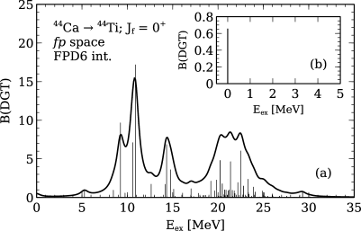
Figure 8: $B(\rm{DGT};0^{+}\rightarrow 0^{+})$ for ⁴⁴Ca as the function of the excitation energy of the final nucleus ⁴⁴Ti (a). The DGT transitions to low-lying states are also shown (b). The strengths were smoothed by using Lorentzian averaging with the width of 1 MeV.

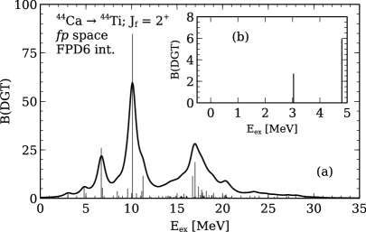
Figure 9: The same as Fig. 8, but for $B(\rm{DGT};0^{+}\rightarrow 2^{+})$.

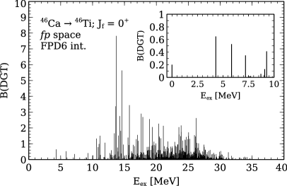
Figure 10: $B(\rm{DGT};0^{+}\rightarrow 0^{+})$ in ⁴⁶Ca.

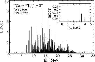
Figure 11: $B(\rm{DGT};0^{+}\rightarrow 2^{+})$ in ⁴⁶Ca.

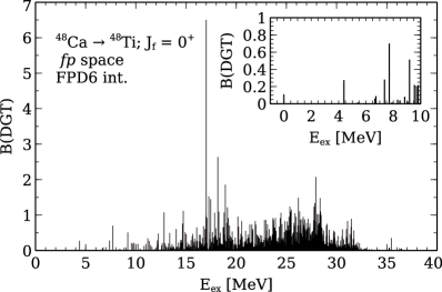
Figure 12: $B(\rm{DGT};0^{+}\rightarrow 0^{+})$ in ⁴⁸Ca.

When the strengths are spread by using the same Lorentzian averaging with the width of 1 MeV to simulate the experimental energy resolution, the results show that the DGT distributions are not single-peaked. The distributions have at least two peaks and in some nuclei as many as four major peaks. We should remind that the single GT resonances have at least two peaks GOODMAN1982241 .

Figs. 13–15 show the dependence of the DGT distributions on the number of intermediate states. We can see that about 100 intermediate states actually contribute to final results in the cases of ⁴⁴Ca (Figs. 13–14). Although the total number of intermediate states in heavier isotopes, including ⁴⁸Ca is many thousands, about 500 intermediate states actually contribute to final results (Fig. 15). The sum rule is useful to determine this number (We remind that the number of intermediate states involved in the calculations for $0\nu\beta\beta$ decay is smaller (see Ref. PhysRevC.88.064312 )).

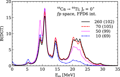
Figure 13: The dependence on the number of intermediate states of $B(\rm{DGT};0^{+}\rightarrow 0^{+})$ in ⁴⁴Ca. The numbers in parentheses are the corresponding total strengths.

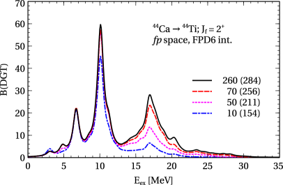
Figure 14: The same as Fig. 13, but for $B(\rm{DGT};0^{+}\rightarrow 2^{+})$ in ⁴⁴Ca.

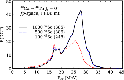
Figure 15: The same as Fig. 13, but for $B(\rm{DGT};0^{+}\rightarrow 0^{+})$ in ⁴⁸Ca.

Fig. 16 and Fig. 17 show the DGT transitions to $J_{f}^{\pi}=0^{+}$ together with the transition to $J_{f}^{\pi}=2^{+}$ in ⁴⁴Ca and ⁴⁶Ca. As one can see the DGT transitions to $J_{f}^{\pi}=2^{+}$ are larger than the transitions to $J_{f}^{\pi}=0^{+}$.

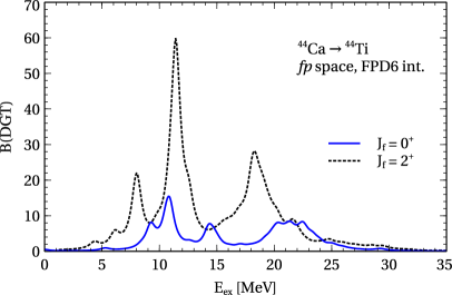
Figure 16: $B(\rm{DGT};0^{+}\rightarrow 0^{+})$ and $B(DGT;0^{+}\rightarrow 2^{+})$ in ⁴⁴Ca.

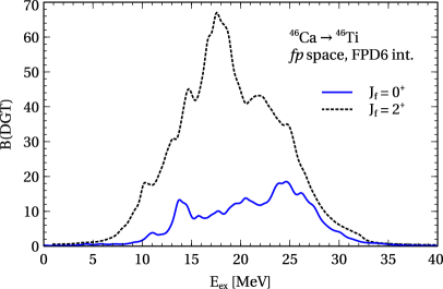
Figure 17: The same as Fig. 16 but for ⁴⁶Ca.

The centroid or average energies of the DGT distributions defined by

$$\overline{E}=\frac{\sum_{f}E_{f}B_{f}(DGT_{-})}{\sum_{f}B_{f}(DGT_{-})}$$ (9)

are given in Table 2. In ⁴⁶Ti, with the FPD6 interaction for example, the average energy for the $J=0^{+}$ is $\overline{E}=21.2$ MeV and for the $J=2^{+}$ it is lower, $\overline{E}=18.0$ MeV. In ⁴⁸Ti the average energy $J=0^{+}$ is $\overline{E}=24.6$ MeV. In Ref. PhysRevLett.120.142502 , a simple relation between the average energy of the ⁴⁸Ca DGT giant resonance and $0\mu\beta\beta$ decay nuclear matrix element was pointed out. The authors conclude that the uncertainties due to the nuclear interaction in the calculation of the DGT distribution in ⁴⁸Ca are relatively under control. In our work, Figs. 18–20 show the DGT distributions are calculated with FPD6 and KB3G interactions. We see that the distributions and the average energies (see Table 2) using FPD6 and KB3G are similar. Our calculated distribution for ⁴⁸Ca is in agreement with the recent result using the same KB3G interaction but a different method (when the factor of three is taken into account). As one can see in Fig. 20 the DGT giant resonance in ⁴⁸Ca is at the energy around 20-30 MeV. In a recent paper Ejiri2017 the experimental results for the double charge-exchange reaction ⁵⁶Fe(¹¹B, ¹¹Li) were presented. In this reaction, several resonances were excited in agreement with the pion DCX studies. In addition, there is a peak at 25 MeV excitation, that the authors indicate that it could be the DGT resonance.

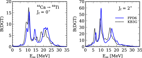
Figure 18: $B(\rm{DGT};0^{+}\rightarrow 0^{+};2^{+})$ in ⁴⁴Ca using FPD6 and KB3G interactions.

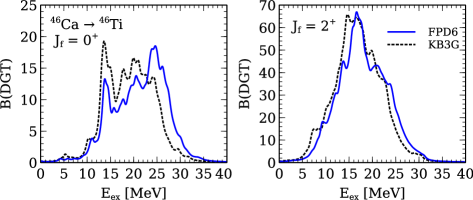
Figure 19: The same as Fig. 18, but for ⁴⁶Ca.

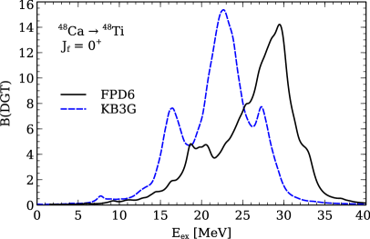
Figure 20: $B(\rm{DGT};0^{+}\rightarrow 0^{+})$ in ⁴⁸Ca using FPD6 and KB3G interactions. The strengths are spread with the width 1 MeV and divided by the factor of 3 for comparing to Ref .PhysRevLett.120.142502 .

In addition, the calculations in the $f$-model space (including the $f_{7/2}$ and the $f_{5/2}$ orbits only) using the same Hamiltonian are given in Fig. 21. For ⁴²Ca, there are two $0^{+}$ DGT states at the excitation energies $0.0$ MeV and $18.3$ MeV. Their strengths are $11.178$ and $13.791$, respectively. There is one $2^{+}$ DGT state at $0.0$ MeV and its strength is $8.658$. Note that the sum rules do not depend on the model space. In the $f$-model space, we obtained exactly the sum rules even for the case of the DGT to $2^{+}$ in ⁴⁸Ca because the calculation can be done without any limitation as now the total number of possible final states is strongly reduced (see Table 2). The DGT distributions in the $f$-model space are much more concentrated. The analytical calculation in the limited $f$-model space helps us know where the DGT strengths concentrate.

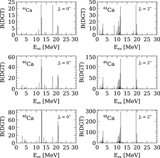
Figure 21: The DGT distributions in the $f$-model space (including the $f_{7/2}$ and the $f_{5/2}$ orbits only) in Calcium isotopes using the FPD6 interaction.

IV Conclusions

The general features and trends of the DGT sum rules in even-$A$ Calcium isotopes are described using the numerical results. The properties of the entire distributions of the DGT are discussed. By studying the stronger DGT transitions, in particular, the DGT giant resonance experimentally and theoretically, the calculations of $\beta\beta$-decay nuclear matrix elements can be calibrated to some extent. There is no doubt that the pion DCX is a sensitive probing tool of nuclear structure. Nowadays the ion DCX reactions have been discussed mainly in the context of $0\nu\beta\beta$, however, the ion DCX reaction itself is a new probing tool of nuclear structure, in particular of spin degrees of freedom. The DGT resonance is just one example. Because two nucleons participate in the DCX reactions with pions or heavy ions, one can expect that the nucleon-nucleon interaction and correlations can be probed, especially for the nucleus that is far from the stability regime.

- (1) I. Navon et al., Phys. Rev. Lett. 52, 105 (1984).
- (2) M. J. Leitch et al., Phys. Rev. Lett. 54, 1482 (1985).
- (3) H. W. Baer et al., Phys. Rev. C 35, 1425 (1987).
- (4) Z. Weinfeld et al., Phys. Rev. C 37, 902 (1988).
- (5) Z. Weinfeld, E. Piasetzky, M. Leitch, H. Baer, C. Mishra, J. Comfort, J. Tinsley, and D. Wright, Phys. Lett. B 237, 33 (1990).
- (6) N. Auerbach, W. R. Gibbs, and E. Piasetzky, Phys. Rev. Lett. 59, 1076 (1987).
- (7) N. Auerbach, W. R. Gibbs, J. N. Ginocchio, and W. B. Kaufmann, Phys. Rev. C 38, 1277 (1988).
- (8) R. Gilman et al., Phys. Rev. C 35, 1334 (1987).
- (9) J. D. Zumbro et al., Phys. Rev. C 36, 1479 (1987).
- (10) S. Mordechai et al., Phys. Rev. Lett. 60, 408 (1988).
- (11) S. Mordechai, N. Auerbach, H. T. Fortune, C. L. Morris, and C. F. Moore, Phys. Rev. C 38, 2709 (1988).
- (12) S. Mordechai et al., Phys. Rev. C 40, 850 (1989).
- (13) S. Mordechai et al., Phys. Rev. C 43, 1111 (1991).
- (14) S. Mordechai et al., Phys. Rev. Lett. 61, 531 (1988).
- (15) S. Mordechai et al., Phys. Rev. C 41, 202 (1990).
- (16) D. L. Watson et al., Phys. Rev. C 43, 1318 (1991).
- (17) S. Mordechai et al., Phys. Rev. C 43, R1509 (1991).
- (18) D. C. Zheng, L. Zamick, and N. Auerbach, Ann. Phys. 197, 343 (1990).
- (19) F. Cappuzzello, M. Cavallaro, C. Agodi, M. Bondì, D. Carbone, A. Cunsolo, and A. Foti, Eur. Phys. J. A 51, 145 (2015).
- (20) F. Cappuzzello, C. Agodi, M. Cavallaro et al., Eur. Phys. J. A 54, 72 (2018).
- (21) N. Auerbach, L. Zamick, and D. C. Zheng, Ann. Phys. 192, 77 (1989).
- (22) T. Uesaka et al., 2015 Riken, RIBF, NP-PAC, NP21512, RIBF141, and private communication.
- (23) K. Takahisa, H. Ejiri, H. Akimune, H. Fujita, R. Matumiya, T. Ohta, T.Shima, M. Tanaka, M. Yosoi, https://arxiv.org/abs/1703.08264v1 (2017).
- (24) K. Muto, Phys. Lett. B 277, 13 (1992).
- (25) N. Shimizu, J. Menéndez, and K. Yako, Phys. Rev. Lett. 120, 142502 (2018).
- (26) B. A. Brown and W. D. M. Rae, Nuclear Data Sheets 120, 115 (2014).
- (27) B. A. Brown, Progress in Particle and Nuclear Physics 47, 517 (2001).
- (28) P. Vogel, M. Ericson, and J. Vergados, Phys. Lett. B 212, 259 (1988).
- (29) D. C. Zheng, L. Zamick, and N. Auerbach, Phys. Rev. C 40, 936 (1989).
- (30) H. Sagawa and T. Uesaka, Phys. Rev. C 94, 064325 (2016).
- (31) W. A. Richter and M. G. Van Der Merwe and R. E. Julies and B. A. Brown, Nucl. Phys. A 523, 325 (1991).
- (32) A. Poves, J. Sánchez-Solano, E. Caurier, and F. Nowacki, Nucl. Phys. A 694, 157 (2001).
- (33) F. Osterfeld, Rev. Mod. Phys. 64, 491 (1992).
- (34) V. Zelevinsky, N. Auerbach, and B. M. Loc, Phys. Rev. C 96, 044319 (2017).
- (35) L. Zamick, D. C. Zheng, and E. M. de Guerra, Phys. Rev. C 39, 2370 (1989).
- (36) B. A. Brown, private communication.
- (37) C. Goodman, Nucl. Phys. A 374, 241 (1982).
- (38) R. A. Sen’kov and M. Horoi, Phys. Rev. C 88, 064312 (2013).