Model-independent Test of the Cosmic Distance Duality Relation

Abstract

A validation of the cosmic distance duality (CDD) relation, $\eta(z)\equiv(1+z)^{2}d_{A}(z)/d_{L}(z)=1$, coupling the luminosity ($d_{L}$) and angular-diameter ($d_{A}$) distances, is crucial because its violation would require exotic new physics. We present a model-independent test of the CDD, based on strong lensing and a reconstruction of the HII galaxy Hubble diagram using Gaussian Processes, to confirm the validity of the CDD at a very high level of confidence. Using parameterizations $\eta(z)=1+\eta_{0}z$ and $\eta(z)=1+\eta_{1}z+\eta_{2}z^{2}$, our best-fit results are $\eta_{0}=0.0147^{+0.056}_{-0.066}$, and $\eta_{1}=0.1091^{+0.1680}_{-0.1568}$ and $\eta_{2}=-0.0603^{+0.0999}_{-0.0988}$, respectively. In spite of these strong constraints, however, we also point out that the analysis of strong lensing using a simplified single isothermal sphere (SIS) model for the lens produces some irreducible scatter in the inferred CDD data. The use of an extended SIS approximation, with a power-law density structure, yields very similar results, but does not lessen the scatter due to its larger number of free parameters, which weakens the best-fit constraints. Future work with these strong lenses should therefore be based on more detailed ray-tracing calculations to determine the mass distribution more precisely.

1 Introduction

The cosmic distance duality (CDD) relation, based on Etherington’s theorem (1933), depends on three essential assumptions: (i) that the spacetime is described by a metric theory of gravity; (ii) that photons travel along null geodesics; and (iii) that their number is conserved along the null geodesics. The CDD is commonly written in the form $\eta(z)=1$, with the definition

$$\eta(z)\equiv(1+z)^{2}\frac{d_{A}(z)}{d_{L}(z)}\ ,$$ (1)

where $d_{A}(z)$ and $d_{L}(z)$ are the angular-diameter and luminosity distances, respectively.

Many attempts have been made to test the validity of the CDD, using several different kinds of data, and/or assumptions. Typically, the angular-diameter distance $d_{A}(z)$ is measured using the angular size of galaxy clusters (Wei et al., 2015; Melia, 2016), while the luminosity distance $d_{L}(z)$ is often inferred from Type Ia SNe. For a non-exhaustive set of references, see Bassett & Kunz (2004); Uzan et al. (2004); Holanda et al. (2010), Holanda et al. (2012); Khedekar & Chakraborti (2011); Li et al. (2011); Nair et al. (2011); Lima et al. (2011); Meng et al. (2012); Ellis et al. (2013); Liao et al. (2016); Yang et al. (2017); Hu & Wang (2018); Melia (2018). But a principal difficulty with using SNe is that the measurement of $d_{L}(z)$ is model-dependent. One can easily see this from the definition of the distance modulus $\mu$, which is given as

$$\mu=5\log d_{L}-5=m_{\mathrm{max}}-M_{\mathrm{max}}\ ,$$ (2)

in terms of the peak magnitude $m_{\mathrm{max}}$ and peak absolute magnitude $M_{\mathrm{max}}$. Every Type Ia SN has almost the same $M_{\mathrm{max}}$, so if $m_{\mathrm{max}}$ is measured, one can obtain the distance modulus $\mu$. The difficulty arises from the scatter in peak magnitudes, which depend rather strongly on the shapes and colors of the SN lightcurves (Guy et al., 2005). To get $m_{\mathrm{max}}$, one of several fitters must be used to parameterize the light curves. For example, one of the most popular parameterizations is (Guy et al., 2007)

$$\mu_{B}(\alpha,\beta,M_{B};z)=m_{B}^{\mathrm{max}}(z)-M_{B}+\alpha x-\beta c\ ,$$ (3)

where $m_{B}^{\mathrm{max}}$ is the rest-frame peak magnitude of the $B$ band, $x$ is the stretch factor that describes the effect of the lightcurve shape on $\mu$, and $c$ is the color parameter representing the influence of intrinsic color and reddening due to dust on $\mu$. The so-called ‘nuisance’ parameters $\alpha$, $\beta$, and $M_{B}$ must be optimized along with all the other parameters in the chosen cosmological model. By now, it is well known that different models are associated with different values of these nuisance variables, so there is no unique way to determine the SN distance moduli in a truly model independent way. It is therefore quite likely that some (or all) of the previously claimed CDD violations may simply be due to unaccounted for influences of the assumed cosmology on $\eta(z)$ (Uzan et al., 2004; Holanda et al., 2010; Li et al., 2011). For a more detailed discussion, see Yang et al. (2013); Melia & Abdelqader (2009); Melia (2012, 2013); Wei et al. (2015); Melia (2018).

In this paper, we steer clear of measurements that require the pre-assumption of particular cosmological models, and instead use strong lenses to measure the ratio of angular-diameter distances, and a reconstruction of the HII galaxy Hubble diagram with Gaussian Processes to obtain the luminosity distance. In the next section, we shall discuss the rationale behind these two kinds of observation, and why one may safely assume model independence in the associated data. Since no model is assumed in any of our analysis, our approach yields a clean measure of the CDD relation.

We shall first briefly summarize the methodology of measuring $\eta(z)$ as a function of redshift using strong lensing and HII galaxies in § 2. We then describe the relevant datasets in § 3, and present the results of our analysis in § 4. We shall demonstrate that this combination of observations confirms the CDD at a very high level of confidence. Finally, we present our conclusions in § 5.

2 Methodology

2.1 Angular-diameter distance from strong lensing

An Einstein ring is formed when the source, lens, and observer are aligned along the same line of sight. For a strong lensing system with a single galaxy as a lens, the Einstein ring’s radius $\theta_{E}$ depends on the ratio of angular-diameter distances between the lens and source, $d_{A}(z_{l},z_{s})$, and the observer and source, $d_{A}(0,z_{s})$, and the mass distribution within the lensing galaxy. The lens galaxy model is sometimes simplified as a single isothermal ellipsoid (SIE) (Ratnatunga et al., 1999; Kochanek et al., 2000). Several prior analyses have shown that a reasonable further simplification may be adequate, in which the ellipsoid is replaced by a sphere (SIS) (Zhang, 2004; Cao et al., 2015; Melia et al., 2015), i.e., with zero ellipticity. To keep the analysis as straightforward as possible, we also adopt this approach for our study in this paper. To gauge the impact of this approximation, however, we shall also compare our results to those obtained with an extended SIE lens model (see § 4.2 below), in which the mass distribution is assumed to be a power-law with optimizable parameters (Koopmans & Mamon, 2005; Cao et al., 2016; Gerhard et al., 2001; Xia et al., 2017).

With the SIS mass distribution, the Einstein radius is expressed as (Schneider et al., 2006; Rana et al., 2017)

$$\theta_{E}=4\pi\frac{d_{A}(z_{l},z_{s})}{d_{A}(0,z_{s})}\left(\frac{\sigma_{\mathrm{SIS}}}{c}\right)^{2}\ ,$$ (4)

where $c$ is the speed of light and $\sigma_{\mathrm{SIS}}$ is the velocity dispersion of the lens mass distribution. Therefore, the quantity that comes directly from observation of a strong lensing system is the distance ratio

$$d_{\mathrm{ratio}} \equiv\frac{d_{A}(z_{l},z_{s})}{d_{A}(0,z_{s})}=\frac{\theta_{E}}{4\pi}\left(\frac{c}{\sigma_{\mathrm{SIS}}}\right)^{2}\ .$$ (5)

In a spatially flat cosmology, one may write for the comoving distance

$$r(z_{l},z_{s})=r(z_{s})-r(z_{l})\;.$$ (6)

Thus, using

$$d_{A}(z)=r(z)/(1+z)\;,$$ (7)

the angular-diameter distance between lens and source, $d_{A}(z_{l},z_{s})$, may be expressed in terms of $d_{A}(z_{l})$ and $d_{A}(z_{s})$:

$$d_{\mathrm{ratio}}=1-\left(\frac{1+z_{l}}{1+z_{s}}\right)\frac{d_{A}(z_{l})}{d_{A}(z_{s})}\ .$$ (8)

Note, however, that for a non-flat cosmology, the comoving distance depends on $\sin$- or $\sinh$-like functions (Räsänen et al., 2015), so a simple relation like Eq. (8) is not possible. Fortunately, most cosmological observations today favor a flat universe (Planck Collaboration et al., 2016), so the spatially flat assumption is not a stringent restriction for our CDD test.

Table 1: Strong-lensing systems used in this paper, sorted by source redshift $z_{s}$

Name	$z_{l}$	$z_{s}$	$\theta_{E}$	Survey	$\sigma_{0}$
			(′′)		(km s-1)
J0219-0829	0.389	2.15	1.3	SL2S	298$\pm$24
J0849-0251	0.274	2.09	1.16	SL2S	279$\pm$35
J0214-0405	0.609	1.88	1.41	SL2S	293$\pm$48
J0217-0513	0.646	1.847	1.27	SL2S	253$\pm$29
J1404+5200	0.456	1.59	2.55	SL2S	342$\pm$20
J0849-0412	0.722	1.54	1.1	SL2S	338$\pm$25
J1406+5226	0.716	1.47	0.94	SL2S	262$\pm$20
J2122+0409	0.626	1.452	1.58	BELLS	326$\pm$56
J0223-0534	0.499	1.44	1.22	SL2S	293$\pm$28
J0830+5116	0.53	1.332	1.14	BELLS	274$\pm$37
J1215+0047	0.642	1.297	1.37	BELLS	266$\pm$46
J0226-0420	0.494	1.232	1.19	SL2S	272$\pm$25
J1631+1854	0.408	1.086	1.63	BELLS	272$\pm$14
J1420+5258	0.38	0.99	0.96	SL2S	252$\pm$24
J2125+0411	0.363	0.978	1.2	BELLS	250$\pm$17
J2303+0037	0.458	0.936	1.02	BELLS	278$\pm$31
J0157-0056	0.513	0.924	0.79	SLACS	308$\pm$49
J0747+5055	0.438	0.898	0.75	BELLS	323$\pm$59
J0747+4448	0.437	0.897	0.61	BELLS	286$\pm$53
J1250+0523	0.232	0.795	1.13	SLACS	257$\pm$14
J1630+4520	0.248	0.793	1.78	SLACS	281$\pm$16
J1531-0105	0.16	0.744	1.71	SLACS	281$\pm$14
J1525+3327	0.358	0.717	1.31	SLACS	264$\pm$26
J1213+6708	0.123	0.64	1.42	SLACS	291$\pm$15
J0037-0942	0.196	0.632	1.53	SLACS	283$\pm$10
J1204+0358	0.164	0.631	1.31	SLACS	275$\pm$17
J1112+0826	0.273	0.63	1.49	SLACS	329$\pm$21
J0324-0110	0.4456	0.6239	0.63	SLACS2017	314$\pm$38
J0946+1006	0.222	0.608	1.38	SLACS	266$\pm$21
J0822+2652	0.241	0.594	1.17	SLACS	264$\pm$15
J0737+3216	0.322	0.581	1	SLACS	339$\pm$17
J1430+4105	0.285	0.575	1.52	SLACS	324$\pm$32
J1020+1122	0.282	0.553	1.2	SLACS	289$\pm$18
J0109+1500	0.294	0.525	0.69	SLACS	259$\pm$20
J0216-0813	0.332	0.524	1.16	SLACS	335$\pm$23
J1627-0053	0.208	0.524	1.23	SLACS	295$\pm$14
J2303+1422	0.155	0.517	1.62	SLACS	254$\pm$16
J1101+1523	0.178	0.5169	1.18	SLACS2017	283$\pm$16
J1205+4910	0.215	0.481	1.22	SLACS	283$\pm$14
J1402+6321	0.205	0.481	1.35	SLACS	268$\pm$17
J0956+5100	0.24	0.47	1.33	SLACS	338$\pm$17
J0955+3014	0.3214	0.4671	0.54	SLACS2017	271$\pm$33
J0935-0003	0.348	0.467	0.87	SLACS	391$\pm$35
J2300+0022	0.228	0.464	1.24	SLACS	285$\pm$17
J1016+3859	0.168	0.439	1.09	SLACS	254$\pm$13
J1106+5228	0.096	0.407	1.23	SLACS	268$\pm$13
J1143-0144	0.106	0.402	1.68	SLACS	264$\pm$13
J1543+2202	0.2681	0.3966	0.78	SLACS2017	288$\pm$16
J0920+3028	0.2881	0.3918	0.7	SLACS2017	293$\pm$17
J1330+1750	0.2074	0.3717	1.01	SLACS2017	251$\pm$12
J0912+0029	0.164	0.324	1.63	SLACS	323$\pm$12
J2324+0105	0.1899	0.2775	0.59	SLACS2017	255$\pm$16
J0044+0113	0.12	0.196	0.79	SLACS	267$\pm$13

2.2 Luminosity distance from GP reconstruction of the HII galaxy Hubble diagram

The hydrogen gas ionized by massive star clusters in HII galaxies emits prominent Balmer lines in $\mathrm{H}\alpha$ and $\mathrm{H}\beta$ (Terlevich & Melnick, 1981; Kunth & Östlin, 2000). The luminosity $L(\mathrm{H}\beta)$ in $\mathrm{H}\beta$ from these structures is strongly correlated with the velocity dispersion $\sigma_{v}$ of the ionized gas (Terlevich & Melnick, 1981), because both the intensity of ionizing radiation and $\sigma_{v}$ increase with the starbust mass (Siegel et al., 2005). The relatively small dispersion in the relationship between $L(\mathrm{H}\beta)$ and $\sigma_{v}$ allows these galaxies and local HII regions to be used as standard candles (Terlevich et al., 2015; Wei et al., 2016; Leaf & Melia, 2018a).

The luminosity of HII galaxies versus their velocity dispersion correlation is (Terlevich et al., 2015)

$$\log L(\mathrm{H}\beta)=\alpha\log\sigma_{v}(\mathrm{H}\beta)+\kappa\ ,$$ (9)

where $\alpha$ and $\kappa$ are constants. As was the case with Type Ia SNe, these two parameters in principle need to be optimized simultaneously with those of the cosmological model. Wei et al. (2016) have shown, however, that their values are insensitive to the adopted model, and appear to be universal. This is the important step that allows us to use the HII galaxy Hubble diagram in a model-independent way. For example, comparing the two distinct cosmologies $R_{\rm h}=ct$ and $\Lambda$CDM, and defining an ‘$H_{0}\text{-}\text{free}$’ logarithmic lumiosity parameter

$$\delta\equiv-2.5\kappa-5\log\left(\frac{H_{0}}{\mathrm{km}\;\mathrm{s}^{-1}\;\mathrm{Mpc}^{-1}}\right)+125.2\ .$$ (10)

Wei et al. (2016) showed that $\alpha=4.86^{+0.08}_{-0.07}$ and $\delta=32.38^{+0.29}_{-0.29}$ for the former, while $\alpha=4.89^{+0.09}_{-0.09}$ and $\delta=32.49^{+0.35}_{-0.35}$ for the latter. Such small differences fall well within the observational uncertainty (note, e.g., that the difference in $\alpha$ is $\sim\sigma/3$). We shall therefore simply use the average values of these ‘nuisance’ parameters, i.e., $\alpha=4.87^{+0.11}_{-0.08}$ and $\delta=32.42^{+0.42}_{-0.33}$. The distance modulus of an HII galaxy is

$$\mu^{\mathrm{obs}}(z)=-\delta+2.5\left[\alpha\log\sigma_{v}(\mathrm{H}\beta)-\log F(\mathrm{H}\beta)\right]\ ,$$ (11)

and the luminosity distance is correspondingly

$$d_{L}^{\mathrm{obs}}(z)=10^{(\mu^{\mathrm{obs}}(z)/5-5)}\;\mathrm{Mpc}\ .$$ (12)

For every $d_{A}(z_{i})$ measurement from a strong-lensing system, we use a model-independent Gaussian Process (GP) reconstruction to get the corresponding $d_{L}(z_{i})$. A description of the GP approach and its use with the HII galaxy Hubble diagram may be found in Yennapureddy & Melia (2017, 2018), based on the pioneering work of Seikel et al. (2012).

It is important to point out an important caveat, however, having to do with possible systematic uncertainties in the HII galaxy probe, specifically the $L(\mathrm{H}\beta)\text{-}\sigma$ correlation, which still needs to be fully understood. Systematic uncertainties in this critical relation include the size of the starburst, its age, the oxygen abundance of HII galaxies and the internal extinction correction (Chávez et al., 2016). The scatter found in the $L(\mathrm{H}\beta)\text{-}\sigma$ relation (Equation  (9)) for HII galaxies suggests that there may exit a possible dependence on a second parameter. Some progress has already been made in trying to mitigate these uncertainties. For example, Chávez et al. (2014) find that for a sample of local HII galaxies, the size of the star-forming region can serve as the second parameter.

Another important consideration is the exclusion of the rotating support for the system (as opposed to purely kinematic support), which would obviously distort the $L(\mathrm{H}\beta)\text{-}\sigma$ relation. Chávez et al. (2014, 2016) have suggested using an upper limit of the velocity dispersion to minimize this possibility, although the catalogue of suitable sources is then greatly reduced. However, even with this limitation, there is no guarantee that this systemic effect will be completely eliminated. Our results in this paper should be viewed with this cautionary consideration, with the hope and expectation that future improvements in our understanding of these systems will make the HII Hubble diagram an even more powerful probe of the integrated distance measure than it is now.

2.3 Measurement of the CDD relation

As one can see from Equations (5) and (8), the lensing measurements provide the values of $\theta_{E}$ and $\sigma_{\mathrm{SIS}}$, which give the ratio of angular-diameter distances to $z_{l}$ and $z_{s}$, i.e. $d_{A}(z_{l})/d_{A}(z_{s})$. For each lens and each source, we then form the ratio given in Equation (1) by calculating the luminosity distance $d_{L}(z_{l})$ and $d_{L}(z_{s})$ from the GP reconstruction of the HII Hubble diagram:

$$\frac{\eta(z_{l})}{\eta(z_{s})} =\frac{(1+z_{l})^{2}}{(1+z_{s})^{2}}\frac{d_{A}(z_{l})}{d_{A}(z_{s})}\frac{d_{L}(z_{s})}{d_{L}(z_{l})}$$

$$=10^{\left[\mu^{\mathrm{obs}}(z_{s})-\mu^{\mathrm{obs}}(z_{l})\right]/5}\left(\frac{1+z_{l}}{1+z_{s}}\right)\times$$

$$\qquad\qquad\left(1-{\theta_{E}\over 4\pi}\left[{c\over\sigma_{\mathrm{SIS}}}\right]^{2}\right).$$ (13)

If the CDD relation is realized in nature, this ratio should always be equal to $1$, independently of $z_{l}$ and $z_{s}$. Our approach uses the strong-lensing and HII galaxy data to ‘measure’ this ratio and test the CDD hypothesis for a broad range of redshift pairs $(z_{l},z_{s})$.

3 Data

We extract our strong lenses from the catalog of 158 sources recently compiled by Leaf & Melia (2018b) (see Table 1 therein.) from the SLACS, BELLS, LSD and SL2S surveys. We keep only strong-lensing systems with $\sigma_{0}\geq 250\,\mathrm{km}\,\mathrm{s}^{-1}$ and $z_{s}\leq 2.33$, which leaves $53$ strong lenses (see Table 1 below). The former condition mitigates the scatter when using the SIS model, while the latter condition is imposed by the limit of the highest redshift in the HII galaxy data, which is $2.33$. The uncertainty in the observed value of $d_{\rm ratio}$ is estimated from the measurement error of the Einstein radius, $\sigma_{\theta_{E}}$, and the velocity dispersion, $\sigma_{\sigma_{0}}$. Using standard error propagation, the corresponding dispersion for $d_{\mathrm{ratio}}$ is

$$\sigma_{d_{\mathrm{ratio}}}=d_{\mathrm{ratio}}\sqrt{\left(\frac{\sigma_{\theta_{E}}}{\theta_{E}}\right)^{2}+4\left(\frac{\sigma_{\sigma_{0}}}{\sigma_{0}}\right)^{2}}\ ,$$ (14)

in which we assume a uniform $5\%$ error for $\sigma_{\theta_{E}}$, following Grillo et al. (2008). There is also the question of how the dispersion $\sigma_{\rm SIS}$ for a SIS model relates to $\sigma_{0}$. Previous work, e.g., by Melia et al. (2015) and Cao et al. (2015), indicates that the statistics of a large sample of lenses is consistent with a SIS model for the lens mass distribution with $\sigma_{\mathrm{SIS}}=\sigma_{0}$. Fits to the data with a more general relation, $\sigma_{\mathrm{SIS}}=f_{e}\sigma_{0}$, with $f_{e}$ a parameter to be optimized, shows that its optimial value is within only a few percentage points of $1$ (Liao et al., 2016).

Nonetheless, recent studies have also shown that a pure SIS model may not be an accurate representation of the lens mass distribution when $\sigma_{0}<250\;\mathrm{km}\;\mathrm{s}^{-1}$ (Leaf & Melia, 2018b) (see Figure 2 therein), for which unphysical values of $d_{\rm ratio}$ are often encountered. Leaf & Melia (2018b) found that ignoring individual variations from a pure SIS structure results in unsatisfactory fitting results. For example, a flattened lens galaxy distribution, corresponding to a small $\sigma_{0}$, deviates significantly from a pure SIS model. To avoid systematics such as this, we shall therefore select from the overall lens sample only those sources with $\sigma_{0}\geq 250\;\mathrm{km}\;\mathrm{s}^{-1}$.

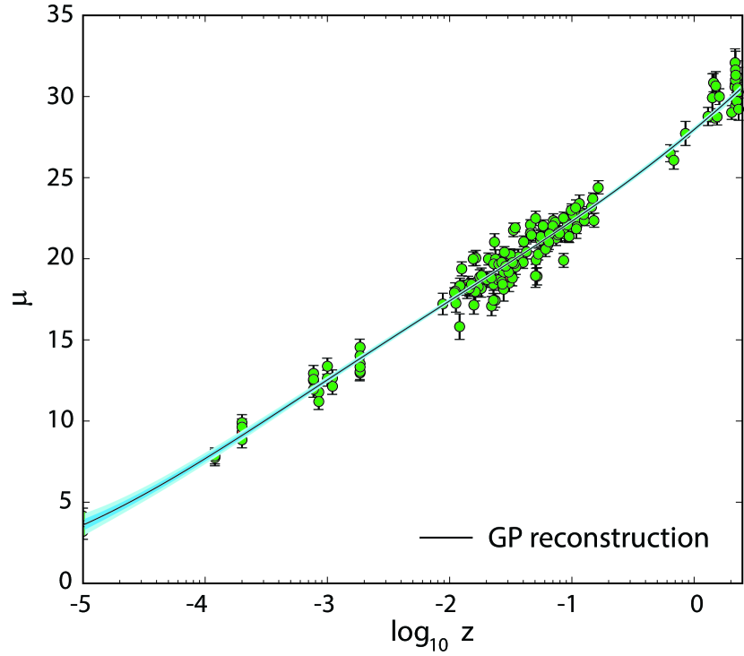
Figure 1: Distance modulus of the currently available HII-region/Galaxy observations, shown with $1\sigma$ error bars, spanning a redshift range up to $\sim 2.33$. The GP reconstructed distance modulus $\mu(z)$ is shown as a solid black curve, with its $1\sigma$ confidence region (shaded swath). (Adapted from Yennapureddy & Melia (2017)). The data sample consists of $25$ high-$z$ HII galaxies, $107$ local HII galaxies, and $24$ giant extragalactic HII regions, for a total of $156$ sources (Terlevich et al., 2015).

For the HII galaxy Hubble diagram, we use the $25$ high-$z$ HII galaxies, $107$ local HII galaxies, and $24$ giant extra galactic HII regions from the catalog compiled by Terlevich et al. (2015). The GP reconstructed distance modulus, $\{z,\;\mu^{\mathrm{obs}}(z),\;\sigma_{\mu^{\mathrm{obs}}}\}$, is calculated from these data following the prescription described and implemented in Yennapureddy & Melia (2017). The distance modulus data and GP reconstruction are shown in figure 1. As one can see in this figure, the error in the reconstructed curve is smaller than that of the individual data points. As discussed more extensively in Yennapureddy & Melia (2017), the confidence region depends on the errors in the data, $\sigma_{\mu_{\mathrm{obs}}}$, on the optimized hyperparameter(s) of the GP method—such as the characteristic ‘bumpiness’ parameter $\sigma_{f}$—and on the product of the covariance matrixes $K_{*}K^{-1}K_{*}^{T}$ between the estimation points and dataset points (see Yennapureddy & Melia (2017)). The reconstructed uncertainty $\sigma_{\mu_{\mathrm{GP}}}(z_{*})$ at the estimation point $z_{*}$ is less than $\sigma_{\mu_{\mathrm{obs}}}$ when, for the point $z_{*}$, there is a large correlation between the data, $K_{*}K^{-1}K_{*}^{T}>\sigma_{f}$, which is most of the time for the HII galaxy data used in this study. As such, the estimated confidence region is smaller than that of the observational data.

The associated $\eta$-ratio errors are estimated from Equation (13) using standard error propagation. Defining

$$k \equiv 10^{[\mu^{\mathrm{obs}}(z_{l})-\mu^{\mathrm{obs}}(z_{s})]/5}\ ,$$ (15)

$$g \equiv\frac{1+z_{l}}{1+z_{s}}(1-d_{\mathrm{ratio}})\ ,$$ (16)

we have

$$\sigma_{k} =k\times\frac{\ln 10}{5}\sqrt{\sigma_{\mu^{\mathrm{obs}}(z_{l})}^{2}+\sigma_{\mu^{\mathrm{obs}}(z_{s})}^{2}}\ ,$$ (17)

$$\sigma_{g} =\frac{1+z_{l}}{1+z_{s}}\sigma_{d_{\mathrm{ratio}}}\ ,$$ (18)

so that

$$\sigma_{\eta(z_{l})/\eta(z_{s})}=\frac{\eta(z_{l})}{\eta(z_{s})}\sqrt{\left(\frac{\sigma_{k}}{k}\right)^{2}+\left(\frac{\sigma_{g}}{g}\right)^{2}}\ .$$ (19)

4 Results and Discussion

4.1 SIS Model

Let us first analyze these data using the simplest SIS model described in § 2.1 above. We shall estimate the impact of changing the mass distribution in the lens by considering an extension to this profile in §4.2. The 53 $\{z_{l},z_{s},\eta(z_{l})/\eta(z_{s})\}$ data points obtained with the use of Equation (13) and the data described in § 3 are plotted as a function of $z_{l}$ in Figure 2, and as a function of $z_{s}$ in Figure 3. As one can see from these distributions, our test of the CDD extends over a significantly large redshift range, with several sources beyond $z_{s}\sim 2$.

To gauge whether these data confirm or reject the CDD, we parameterize $\eta(z)$ using the following two forms:

$$\eta(z) =1+\eta_{0}z\ ,$$ (20)

$$\eta(z) =1+\eta_{1}z+\eta_{2}z^{2}\ ,$$ (21)

in which $\eta_{0},\;\eta_{1}$ and $\eta_{2}$ are all assumed to be constant. The CDD corresponds to $\eta(z)\equiv 1$, i.e., $\eta_{0}=\eta_{1}=\eta_{2}=0$.

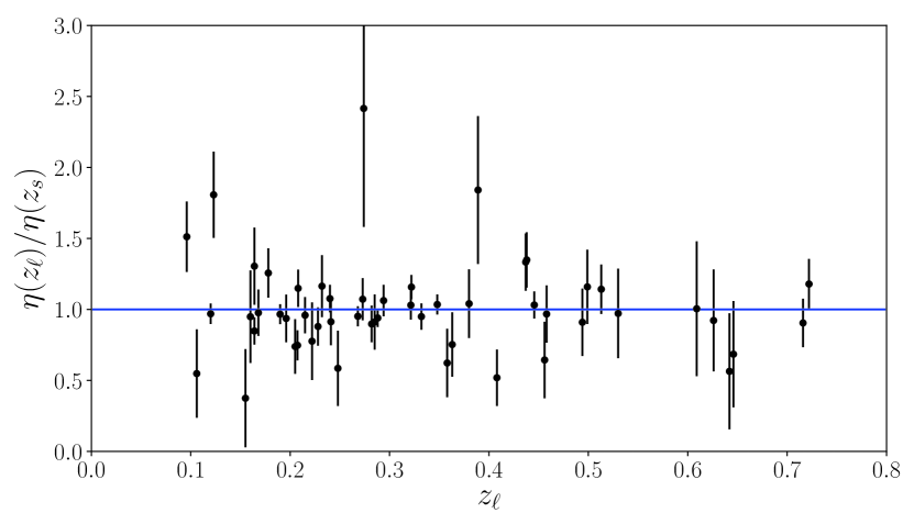
Figure 2: Measured values of the ratio $\eta(z_{l})/\eta(z_{s})$ versus $z_{\ell}$, estimated from strong lensing systems and the GP reconstruction of the HII galaxy Hubble diagram. These data confirm the CDD at a very high level of confidence.

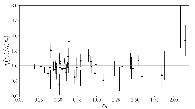
Figure 3: Measured values of the ratio $\eta(z_{l})/\eta(z_{s})$ versus $z_{s}$, estimated from strong lensing systems and the GP reconstruction of the HII galaxy Hubble diagram. These data confirm the CDD at a very high level of confidence.

To find the best-fitting CDD parameters and the confidence regions, we use Bayesian statistical methods and the Markov chain Monte Carlo (MCMC) technique to calculate the posterior probability density function (PDF) of the parameter matrix $\bm{\eta}\equiv\{\eta_{0}\}\ \mathrm{or}\ \{\eta_{1},\eta_{2}\}$, which is

$$p(\bm{\eta}|\text{eta ratio data})\propto\mathcal{L}(\bm{\eta},\text{eta ratio data})\times p(\bm{\eta})\ ,$$ (22)

where

• $p(\bm{\eta})$ is the prior and (assumed) uniform distribution;

• $\mathcal{L}\propto\exp(-\chi^{2}/2)$ is the likelihood function, and

  $$\chi^{2}=\sum_{i}\left\{\frac{\left[\eta(z_{l,i})/\eta(z_{s,i})\right]^{\text{obs}}-\eta(\bm{\eta};z_{l})/\eta(\bm{\eta};z_{s})}{\sigma_{\eta(z_{l,i})/\eta(z_{s,i})}}\right\}^{2}$$ (23)

  is the $\chi^{2}$ function, with $\eta(\bm{\eta};z)\equiv 1+\eta_{0}z$ or $1+\eta_{1}z+\eta_{2}z^{2}$, as the case may be.

The MCMC method uses the Metropolis-Hastings algorithm to generate Markov chains of sample points in parameter space from the posterior probability (Ivezić et al., 2014). We use the emcee Python module (Foreman-Mackey et al., 2013) that implements Markov chain Monte Carlo to sample from the posterior distribution of parameters ($\eta_{0}$, or $\eta_{1}$ and $\eta_{2}$). For the two sets of data used in this analysis, we find that the optimized values of the parameters in $\eta(z)$, and their $1\sigma$ errors, are

$$\eta_{0} =0.0147^{+0.056}_{-0.066}\ ,$$ (24)

$$\eta_{1} =0.1091^{+0.1680}_{-0.1568}\ ,\quad\eta_{2}=-0.0603^{+0.0999}_{-0.0988}\ .$$ (25)

The PDF plots are shown in Figure 4 and 5. The contours were plotted using the Python package “GetDist”. As one can see, the best-fit values of both $\eta_{0}$, and $\eta_{1}$ and $\eta_{2}$, are entirely consistent with the CDD at a very high level of confidence. Specifically, the strong lensing data, in combination with the HII galaxy Hubble diagram, show that $\eta_{0}$ deviates from zero by less than $\sim\sigma/4$, while $\eta_{1}$ and $\eta_{2}$ deviate from zero by less than $\sim 2\sigma/3$.

Notice, however, that the parameterization in Equation (20) appears to give a more accurate result than that in Equation (21). A quick inspection of Figures 2 and 3 suggests why the simpler parameterization in the former appears to confirm the CDD more strongly than that in the latter. Though the $\eta(z_{l})/\eta(z_{s})$ data points fluctuate across $\eta(z)=1$ throughout the redshift range of interest, some points clearly deviate from this value by $1\sigma-2\;\sigma$. This scatter produces enhanced fluctuation in the redshift dependence of the parameterized $\eta(z)$ function when a higher-order polynomial is used, which accounts for the fact that both $\eta_{1}$ and $\eta_{2}$ differ from zero by a larger fraction of their $\sigma$ than does $\eta_{0}$.

Unfortunately, this residual scatter is due to the over-simplifying assumption that all lens mass distributions follow the SIS, as noted earlier by Leaf & Melia (2018b). For example, all lens systems with $d_{A}(z_{l})>d_{A}(z_{s})$—which is clearly unphysical—have a small velocity dispersion $\sigma_{0}\leq 233\,\mathrm{km}\,\mathrm{s}^{-1}$. And, as shown in Figure 2 of Leaf & Melia (2018b), there is an obvious correlation between the velocity dispersion $\sigma_{0}$ and $d_{\mathrm{ratio}}$, i.e., a correlation between the mass distribution of the lens galaxy and the lens and source’s distance ratio, which cannot be accounted for in the SIS model. This significant correlation is a hint that the SIS approximation is reliable only for strong lensed systems. We have largely mitigated this effect by restricting our analysis to systems with $\sigma_{0}\geq 250$ km s^-1, but variations away from the pure SIS model are apparently present even for this reduced sample. Our results already provide compelling evidence that the CDD is realized in nature, but we suggest that a parameterization such as that in Equation (21) can do even better in the future if the lens mass distribution were to be determined more accurately (say, with ray tracing), rather than the adoption of a simple SIS model.

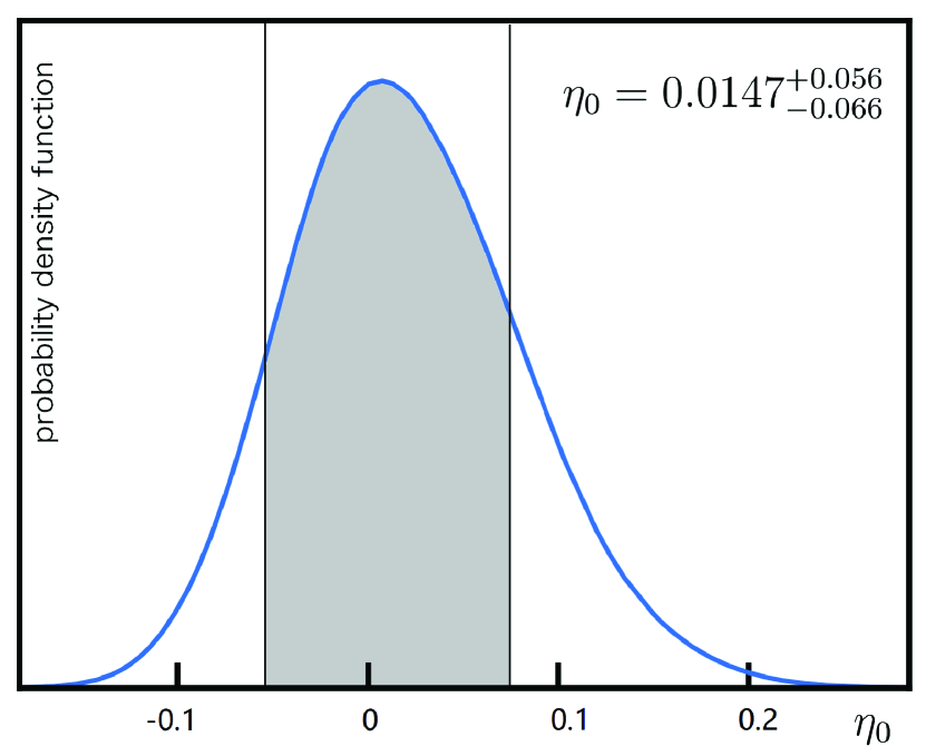
Figure 4: Posterior probability density function of the parameter $\eta_{0}$ in the CDD parameterization $\eta(z)=1+\eta_{0}z$. Its optimized value is consistent with $0$ to within $\sim\sigma/4$.

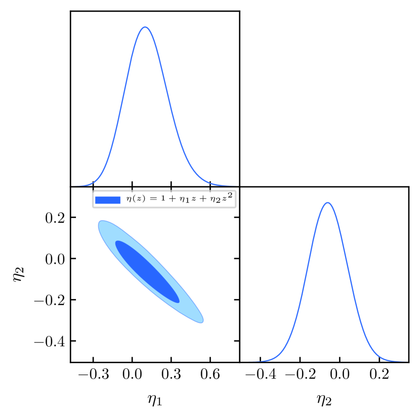
Figure 5: Posterior probability density function of the parameters $\eta_{1}$ and $\eta_{2}$ in the CDD parameterization $\eta(z)=1+\eta_{1}z+\eta_{2}z^{2}$. Both of the optimized values are consistent with $0$ at better than $\sim 2\sigma/3$.

Of course, the uncertainties of the HII galaxy data that provide the luminosity distance also contribute to the $\eta$-ratio’s scatter. But as one can see from Figure 1 and the discussion of the GP reconstruction in Section 3, the relative uncertainty in the GP reconstructed HII galaxy distance modulus is much smaller than that of the strong lensing data. The dominant contribution to the error in Equation  (19) therefore comes from the lens data rather than the HII galaxy data.

4.2 Extended SIE Model

As noted earlier, we can explore this hypothesis further by examining how a change in the lens model affects the scatter seen in figs. 2 and 3. To do so, however, we need to rexamine how one converts the observable quantities of strong lensing systems, such as the Einstein radius $\theta_{E}$ and the central velocity dispersion $\sigma$ of the lensing galaxy, into the angular-diameter distance. For the SIS model, the relation between these observables and $d_{A}$ is Equation (4) or (5). The simplest SIE model introduced a phenomenological parameter $f_{e}$ to account for any possible difference between the true velocity dispersion and that of the SIS model:

$$\theta_{E}=4\pi\frac{d_{A}(z_{l},z_{s})}{d_{A}(0,z_{s})}\left(\frac{f_{e}\sigma}{c}\right)^{2}$$ (26)

but, as mentioned in § 3, the optimal value of $f_{e}$ is very close to $1$ so it does not provide any effective variation away from a pure SIS.

To understand the influence of the lensing galaxy’s mass distribution on our CDD test, we therefore also consider an extended SIE model based on an assumed power-law density profile $\rho(r)$ and a luminosity density of stars $\nu(r)$ (Koopmans & Mamon, 2005):

$$\rho(r) =\rho_{0}\left(\frac{r}{r_{0}}\right)^{-\tau}\ ,$$ (27)

$$\nu(r) =\nu_{0}\left(\frac{r}{r_{0}}\right)^{-\gamma}\ ,$$ (28)

where $r$ is the spherical radial coordinate from the center of the lensing galaxy; and $\tau$ and $\gamma$ are adjustable free parameters. The observed velocity dispersion $\sigma_{0}$ can provide a dynamical estimate of the mass, based on this power-law density profile. The corresponding central velocity disperion of the extended-SIE model is (Cao et al., 2016)

$$\sigma_{\text{ex-SIE}}^{2}= \left(\frac{c^{2}}{4}\frac{d_{A}(0,z_{s})}{d_{A}(z_{l},z_{s})}\theta_{E}\right)\frac{2}{\sqrt{\pi}(\xi-2\beta)}\left(\frac{\theta_{\mathrm{ap}}}{\theta_{E}}\right)^{2-\tau}$$

$$\times\left[\frac{\lambda(\xi)-\beta\,\lambda(\xi+2)}{\lambda(\tau)\,\lambda(\gamma)}\right]\frac{\Gamma(3-\xi/2)}{\Gamma(3-\gamma/2)}\ ,$$ (29)

where

• $\beta$ characterizes the anisotropic distribution of the three-dimensional velocity dispersion, which appears to be Gaussian with $\beta=0.18\pm 0.13$, based on a sample of local elliptical galaxies (Gerhard et al., 2001);

• $\theta_{\mathrm{ap}}$ is the spectrometer aperture radius;

• $\xi\equiv\tau+\gamma-2$;

• $\lambda(x)\equiv\Gamma\left(\frac{x-1}{2}\right)\Big{/}\Gamma\left(\frac{x}{2}\right)$ is the ratio of Euler’s gamma functions.

We use the distances $d_{A}(0,z_{s})$ and $d_{A}(z_{l},z_{s})$ to extract $\sigma$ from the above equation, with the help of the CDD relation $d_{A}(z)={d_{L}(z)\,\eta(z)}/{(1+z)^{2}}$ and the HII galaxy data. The result is

$$\frac{d_{A}(0,z_{s})}{d_{A}(z_{l},z_{s})} =\frac{1}{d_{\mathrm{ratio}}}=\left[1-\frac{1+z_{l}}{1+z_{s}}\frac{d_{A}(z_{l})}{d_{A}(z_{s})}\right]^{-1}$$ (30)

$$=\left[1-\frac{1+z_{s}}{1+z_{l}}\frac{\eta(z_{l})}{\eta(z_{s})}\frac{d_{L}(z_{l})}{d_{L}(z_{s})}\right]^{-1}$$ (31)

$$=\left[1-\frac{1+z_{s}}{1+z_{l}}\frac{\eta(z_{l})}{\eta(z_{s})}10^{(\mu^{\mathrm{obs}}(z_{l})-\mu^{\mathrm{obs}}(z_{s}))/5}\right]^{-1}\ .$$ (32)

But notice that we now have two more free parameters (i.e., $\tau$ and $\gamma$) in the extended SIE model, than we did with the simple SIS. The overall number of adjustable variables is now large enough to create degeneracy in the optimization. As such, we restrict our attention solely to the formulation $\eta(z)=1+\eta_{0}z$ (i.e., Eq. 20) to mitigate this excessive flexibility.

Our optimization strategy now relies on identifying the best-fit values of $\tau$ and $\gamma$, for which the relevant $\chi^{2}$ function is

$$\chi^{2}=\sum_{i=1}^{53}\left[\frac{\sigma^{\text{ex-SIE}}_{i}(\tau,\gamma,\beta;\eta_{0})-\sigma_{i}^{\mathrm{obs}}}{\sigma_{\sigma_{0,i}}}\right]^{2}\ ,$$ (33)

where the sum is taken over the 53 strong lens systems identified in Table 1 above.

The 1D and 2D marginalized distribution plots produced with this procedure are shown in fig. 6 for the CDD parameter $\eta_{0}$ and the power-law indices $\tau$ and $\gamma$. The corresponding $68\%$ confidence limits are

$$\eta_{0} =0.0093^{+0.1520}_{-0.0939}\ ,$$ (34)

$$\tau =1.8990^{+0.0521}_{-0.0526}\ ,$$ (35)

$$\gamma =2.3680^{+0.1185}_{-0.1305}\ .$$ (36)

Our optimized values of $\tau$ and $\gamma$ are consistent with those found in previous work Xia et al. (2017), in which the reported results were $\tau=1.97\pm 0.04$ and $\gamma=2.40\pm 0.13$. We note that Xia et al. (2017) used the model dependent Type Ia SN data with the CDD to extract the angular-diameter distance, whereas we have used the HII galaxy Hubble diagram, yet the use of an optimized power-law lens model has not changed the outcome significantly. The best-fit value of $\eta_{0}$ is still fully consistent with the CDD, but the confidence limit is much wider than that of a pure SIS model (compare Eqs. 24 and 34). This slight weakening of the CDD constraint is entirely due to the larger number of free parameters in the extended SIE model. We conclude from this comparison that the use of a more elaborate SIE lens model (such as the extended power-law profile we have examined here) will probably not improve the results we have obtained with a simple SIS, in spite of the lingering scatter associated with this simplified mass profile (see figs. 2 and 3). A more direct empirical determination of the mass distribution within the lenses will be required to significantly refine the results reported here.

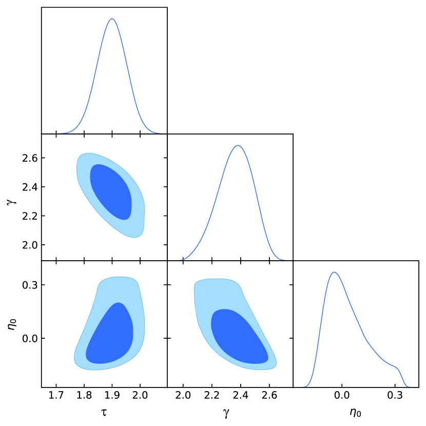
Figure 6: Posterior probability density function of the parameter $\eta_{0}$, and the power-law lens model indices $\tau$ and $\gamma$.

5 Conclusion

A commonly used method of testing the CDD has been to compare the luminosity distance derived from Type Ia SNe with the angular-diameter distance measured using galaxy clusters. But these are no longer the only standard candles and rulers available today. Seeking alternatives is desirable because the older approach requires the pre-assumption of specific cosmological models in order to optimize the ‘nuisance’ parameters in the distance-redshift relation. This limiting factor can lead to additional uncertainty and bias, which may explain why some earlier work with the CDD has produced conflicting results. A summary of previous inconsistencies may be found in Melia (2018).

In this paper, we have chosen a new combination of standard candles (HII galaxies) and rulers (strong lenses) to test the CDD without the need to pre-assume any particular cosmology. The fact that our analysis shows consistency with the CDD at a very high level of confidence is therefore quite compelling because we have avoided introducing unknown systematics associated with particular models. We do note, however, that we have assumed spatial flatness throughout our analysis, which appears to be consistent with a broad range of cosmological measurements. Nevertheless, this is a caveat to keep in mind, should any new evidence emerge that the Universe is not spatially flat.

Another important benefit of our model-independent study is that the additional flexibility in fitting the data otherwise present when cosmology-dependent parameterizations are introduced is absent from our approach. Our test is therefore straightforward and clean because any possible variations in $\eta(z)$ away from $1$ cannot be attributed to the cosmology itself. Were we to find that $\eta(z)\neq 1$, the evidence in favor of new physics would therefore have been stronger with our method than what would be found using model-dependent data.

The results in this paper fully confirm another recent model-independent test of the CDD carried out by Melia (2018). In that work, the standard ruler was provided by compact quasar cores. We are therefore starting to see a consistent pattern of results in which model-independent tests all agree that the CDD is realized in nature.

The principal caveat of our work is the irreducible scatter in our CDD data stemming from the use of a simplified single isothermal sphere (SIS) model for the lens. We have attempted to mitigate the impact of an imprecisely known mass distribution in the lens by also considering an extended SIE model, in which the internal structure of the lens is characterized by power laws for the mass and luminosity densities, with two adjustable indices. While this allows greater freedom in modeling the lens itself, however, the downside with such an approach is the additional degeneracy offered by the greater flexibility with the overall optimization of the parameters. Our results for both the simple SIS and the extended SIE lens models confirm the CDD all the way out to $z\sim 2.3$, with a violation no bigger than $\eta_{0}\sim 0.01-0.015$, in a parameterization $\eta(z)=1+\eta_{0}z$. But the CDD constraint is actually weaker with the extended SIE lens (i.e., $\eta_{0}=0.0093^{+0.1520}_{-0.0939}$ versus $\eta_{0}=0.0147^{+0.056}_{-0.066}$) due to the less precise confidence range of the best fit values resulting from the adjustable power-law distributions.

In future work with strong lensing, it would be desirable to determine the lens mass distribution more accurately, e.g., using ray tracing, rather than simply relying on a SIS model, which appears to produce irreducible scatter in the results due to its over-simplification of the lens structure. Eventually, this improvement should yield a better measurement of the angular-diameter distance, allowing us to test the CDD with even higher precision than is available today.

References

- Bassett & Kunz (2004) Bassett, B. A., & Kunz, M. 2004, Phys. Rev. D, 69, 101305, doi: 10.1103/PhysRevD.69.101305
- Cao et al. (2015) Cao, S., Biesiada, M., Gavazzi, R., Piórkowska, A., & Zhu, Z.-H. 2015, ApJ, 806, 185, doi: 10.1088/0004-637X/806/2/185
- Cao et al. (2016) Cao, S., Biesiada, M., Yao, M., & Zhu, Z.-H. 2016, Monthly Notices of the Royal Astronomical Society, 461, 2192, doi: 10.1093/mnras/stw932
- Chávez et al. (2016) Chávez, R., Plionis, M., Basilakos, S., et al. 2016, Monthly Notices of the Royal Astronomical Society, 462, 2431, doi: 10.1093/mnras/stw1813
- Chávez et al. (2014) Chávez, R., Terlevich, R., Terlevich, E., et al. 2014, Monthly Notices of the Royal Astronomical Society, 442, 3565, doi: 10.1093/mnras/stu987
- Ellis et al. (2013) Ellis, G. F. R., Poltis, R., Uzan, J.-P., & Weltman, A. 2013, Phys. Rev. D, 87, 103530, doi: 10.1103/PhysRevD.87.103530
- Etherington (1933) Etherington, I. 1933, The London, Edinburgh, and Dublin Philosophical Magazine and Journal of Science, 15, 761
- Foreman-Mackey et al. (2013) Foreman-Mackey, D., Hogg, D. W., Lang, D., & Goodman, J. 2013, PASP, 125, 306, doi: 10.1086/670067
- Gerhard et al. (2001) Gerhard, O., Kronawitter, A., Saglia, R. P., & Bender, R. 2001, The Astronomical Journal, 121, 1936
- Grillo et al. (2008) Grillo, C., Lombardi, M., & Bertin, G. 2008, A&A, 477, 397, doi: 10.1051/0004-6361:20077534
- Guy et al. (2005) Guy, J., Astier, P., Nobili, S., Regnault, N., & Pain, R. 2005, A&A, 443, 781, doi: 10.1051/0004-6361:20053025
- Guy et al. (2007) Guy, J., Astier, P., Baumont, S., et al. 2007, A&A, 466, 11, doi: 10.1051/0004-6361:20066930
- Holanda et al. (2010) Holanda, R. F. L., Lima, J. A. S., & Ribeiro, M. B. 2010, ApJ, 722, L233, doi: 10.1088/2041-8205/722/2/L233
- Holanda et al. (2012) Holanda, R. F. L., Lima, J. A. S., & Ribeiro, M. B. 2012, A&A, 538, A131, doi: 10.1051/0004-6361/201118343
- Hu & Wang (2018) Hu, J., & Wang, F. Y. 2018, MNRAS, 477, 5064, doi: 10.1093/mnras/sty955
- Ivezić et al. (2014) Ivezić, Ž., Connelly, A. J., VanderPlas, J. T., & Gray, A. 2014, Statistics, Data Mining, and Machine Learning in Astronomy
- Khedekar & Chakraborti (2011) Khedekar, S., & Chakraborti, S. 2011, Phys. Rev. Lett., 106, 221301, doi: 10.1103/PhysRevLett.106.221301
- Kochanek et al. (2000) Kochanek, C. S., Falco, E. E., Impey, C. D., et al. 2000, The Astrophysical Journal, 543, 131
- Koopmans & Mamon (2005) Koopmans, L., & Mamon, G. 2005, Proc. of XXIst IAP Coll. Mass Profiles Shapes of Cosmological Structures, EDP Sciences France
- Kunth & Östlin (2000) Kunth, D., & Östlin, G. 2000, Astronomy and Astrophysics Review, 10, 1, doi: 10.1007/s001590000005
- Leaf & Melia (2018a) Leaf, K., & Melia, F. 2018a, Monthly Notices of the Royal Astronomical Society, 474, 4507, doi: 10.1093/mnras/stx3109
- Leaf & Melia (2018b) Leaf, K., & Melia, F. 2018b, Monthly Notices of the Royal Astronomical Society, sty1365, doi: 10.1093/mnras/sty1365
- Li et al. (2011) Li, Z., Wu, P., & Yu, H. 2011, The Astrophysical Journal Letters, 729, L14
- Liao et al. (2016) Liao, K., Li, Z., Cao, S., et al. 2016, ApJ, 822, 74, doi: 10.3847/0004-637X/822/2/74
- Lima et al. (2011) Lima, J. A. S., Cunha, J. V., & Zanchin, V. T. 2011, ApJ, 742, L26, doi: 10.1088/2041-8205/742/2/L26
- Melia (2012) Melia, F. 2012, The Astronomical Journal, 144, 110 doi: 10.1088/0004-6256/144/4/110
- Melia (2013) Melia, F. 2013, The Astrophysical Journal, 764, 72 doi: 10.1088/0004-637X/764/1/72
- Melia (2016) Melia, F. 2016, Proceedings of the Royal Society of London A: Mathematical, Physical and Engineering Sciences, 472, doi: 10.1098/rspa.2015.0765
- Melia (2018) Melia, F. 2018, ArXiv e-prints, arXiv:1804.09906. https://arxiv.org/abs/1804.09906
- Melia & Abdelqader (2009) Melia, F. & Abdelqader, M. 2009, IJMP-D, 18, 1889 doi: 10.1142/S0218271809015746
- Melia et al. (2015) Melia, F., Wei, J.-J., & Wu, X.-F. 2015, AJ, 149, 2, doi: 10.1088/0004-6256/149/1/2
- Meng et al. (2012) Meng, X.-L., Zhang, T.-J., Zhan, H., & Wang, X. 2012, ApJ, 745, 98, doi: 10.1088/0004-637X/745/1/98
- Nair et al. (2011) Nair, R., Jhingan, S., & Jain, D. 2011, Journal of Cosmology and Astroparticle Physics, 2011, 023
- Planck Collaboration et al. (2016) Planck Collaboration, Ade, P. A. R., Aghanim, N., et al. 2016, A&A, 594, A13, doi: 10.1051/0004-6361/201525830
- Rana et al. (2017) Rana, A., Jain, D., Mahajan, S., Mukherjee, A., & Holanda, R. F. L. 2017, Journal of Cosmology and Astro-Particle Physics, 2017, 010, doi: 10.1088/1475-7516/2017/07/010
- Räsänen et al. (2015) Räsänen, S., Bolejko, K., & Finoguenov, A. 2015, Phys. Rev. Lett., 115, 101301, doi: 10.1103/PhysRevLett.115.101301
- Ratnatunga et al. (1999) Ratnatunga, K. U., Griffiths, R. E., & Ostrander, E. J. 1999, AJ, 117, 2010, doi: 10.1086/300840
- Schneider et al. (2006) Schneider, P., Kochanek, C., & Wambsganss, J. 2006, Gravitational lensing: strong, weak and micro: Saas-Fee advanced course 33, Vol. 33 (Springer Science & Business Media)
- Seikel et al. (2012) Seikel, M., Clarkson, C., & Smith, M. 2012, Journal of Cosmology and Astro-Particle Physics, 2012, 036, doi: 10.1088/1475-7516/2012/06/036
- Siegel et al. (2005) Siegel, E. R., Guzmán, R., Gallego, J. P., Orduña López, M., & Rodríguez Hidalgo, P. 2005, MNRAS, 356, 1117, doi: 10.1111/j.1365-2966.2004.08539.x
- Terlevich & Melnick (1981) Terlevich, R., & Melnick, J. 1981, Monthly Notices of the Royal Astronomical Society, 195, 839, doi: 10.1093/mnras/195.4.839
- Terlevich et al. (2015) Terlevich, R., Terlevich, E., Melnick, J., et al. 2015, MNRAS, 451, 3001, doi: 10.1093/mnras/stv1128
- Uzan et al. (2004) Uzan, J.-P., Aghanim, N., & Mellier, Y. 2004, Phys. Rev. D, 70, 083533, doi: 10.1103/PhysRevD.70.083533
- Wei et al. (2015) Wei, J.-J., Wu, X.-F., & Melia, F. 2015, Monthly Notices of the Royal Astronomical Society, 447, 479, doi: 10.1093/mnras/stu2470
- Wei et al. (2016) Wei, J.-J., Wu, X.-F., & Melia, F. 2016, Monthly Notices of the Royal Astronomical Society, 463, 1144, doi: 10.1093/mnras/stw2057
- Wei et al. (2015) Wei, J.-J., Wu, X.-F., Melia, F., & Maier, R. S. 2015, AJ, 149, 102, doi: 10.1088/0004-6256/149/3/102
- Xia et al. (2017) Xia, J.-Q., Yu, H., Wang, G.-J., et al. 2017, The Astrophysical Journal, 834, 75
- Yang et al. (2017) Yang, T., Holanda, R. F. L., & Hu, B. 2017, ArXiv e-prints. https://arxiv.org/abs/1710.10929
- Yang et al. (2013) Yang, X., Yu, H.-R., Zhang, Z.-S., & Zhang, T.-J. 2013, ApJ, 777, L24, doi: 10.1088/2041-8205/777/2/L24
- Yennapureddy & Melia (2017) Yennapureddy, M. K., & Melia, F. 2017, Journal of Cosmology and Astro-Particle Physics, 2017, 029, doi: 10.1088/1475-7516/2017/11/029
- Yennapureddy & Melia (2018) Yennapureddy, M. K., & Melia, F. 2018, European Physical Journal C, 78, 258, doi: 10.1140/epjc/s10052-018-5746-8
- Zhang (2004) Zhang, T.-J. 2004, ApJ, 602, L5, doi: 10.1086/382480