A note on cosmological features of modified Newtonian potentials

Abstract

Considering some modified Newtonian potentials and the Hubble law in writing the total energy of a test mass located at the edge of a flat Friedmann-Robertson-Walker universe, we obtain several modified Friedmann equations. Interestingly enough, our study shows that the employed potentials, while some of them have some successes in modelling the spiral galaxies rotation curves, may also address an accelerated universe. This fact indicates that dark energy and dark matter may have some common origins and aspects.

I Introduction

One of the interesting problems in cosmology is seeking for modified forms of the Newtonian potential which can cover the results of the general relativity (GR) in the Newtonian framework nc6 ; ncprd ; fes ; yc1 ; yc2 ; yc4 ; yc5 ; yc6 ; yc7 ; yc8 ; yc9 ; roos ; ybh ; ej ; yp ; m1 ; m2 ; m3 ; m4 ; m5 ; m6 ; m7 ; m8 ; ref1 . A famous example, which originally returns to Newton, is m1 ; m2

$$V\left(r\right)=\left(A+\frac{B}{r}\right)V_{\mathrm{N}}\left(r\right),\text{ Type A}$$ (1)

where $V_{\mathrm{N}}\left(r\right)=-GmM/r$ denotes the Newtonian potential and $A$ and $B$ are unknown parameters found by either fitting with the observations m1 ; m2 ; m3 ; m4 ; m5 ; m6 ; m7 ; m8 or using other parts of physics m9 . In cosmological setup, without working in the GR framework, one can still get the Friedmann equations by using the Hubble law and the Newtonian potential in order to write the total energy of a test particle located at the edge of the Friedmann-Robertson-Walker (FRW) universe nm ; nc1 ; nc2 ; nc20 ; nc6 ; nc4 ; nc5 ; ncprd ; roos . Nevertheless, the Newtonian potential cannot provide suitable description for some questions such as the backreaction, dark matter and dark energy problems ncprd ; roos ; nc6 and one needs alternative theories of Newtonian gravity to avoid these difficulties ncprd .

In fact, due to pointed out problems, modified versions of the Newtonian potential such as the Yukawa potential yp have been employed. These potentials lead to interesting results in describing gravitational phenomena ncprd ; fes ; yc1 ; yc2 ; yc4 ; yc5 ; yc6 ; yc7 ; yc8 ; yc9 ; ybh ; ej . Amonog different kinds of modified potentials, the below ones have attracted more attentions in studying the gravitational systems fes ; yc1 ; yp ; ybh ; ej ; m1

$$V\left(r\right)=\left\{\begin{array}[]{ll}V_{\mathrm{N}}\left(r\right)e^{-\alpha r},&\text{Type B}\\ &\\ \left(1+\beta e^{-\alpha r}\right)V_{\mathrm{N}}\left(r\right)&\text{Type C}\end{array}\right.$$ (2)

where $\alpha$ and $\beta$ are some constants. The possible ranges for the values of $\alpha$ and $\beta$ depend on the system. These potentials can support some kinds of black holes ybh . It is also useful to mention that the potentials such as Type C can be obtained either by looking for the Newtonian limits of some modified GR theories yc31 ; yc32 ; yc3 or taking the probable non-local features of the Newtonian gravity into account ynl . Further corrections to the Newtonian potential such as the logarithmic modifications can be found in Refs. ynl ; log1 ; log2 ; log3 ; r1 . The latter correction can successfully describe the spiral galaxies rotation curves. It is also useful to mention here that the gravitational wave (GW) astronomy is a very powerful tool to find out the more comprehensive gravitational theory corda1 ; corda2 .

The ability of the mentioned potentials to describe the current accelerated universe has not been studied yet. So, the question whether the modifications to the Newtonian potential can provide a classical description for the dark energy remains unrevealed. In addition to this query, it is also interesting to study the cosmological consequences of the above potentials to figure out if they can provide acceptable descriptions for various gravitational systems ncprd ; yc1 ; yc2 ; yc4 ; yc5 ; yc6 ; yc7 ; yc8 ; yc9 ; fes ; ybh ; ej ; m1 ; m2 ; m3 ; m4 ; m5 ; m6 ; m7 ; m8 ; m9 .

In the next section, we introduce and study three sets of modified Friedmann equations corresponding to the above introduced potentials. Next, in Sec. III, after addressing a Hook correction to the Newtonian potential and investigating some of its properties, the cosmological consequences of a logarithmic modified Newtonian potential will be studied. The last section is devoted to the summary and conclusion. Throughout this paper, dot denotes the derivative with respect to time and we set $c=\hbar=1$.

II Modified Newtonian models and dark energy

Consider an expanding box with radius $R$, filled by a fluid with energy density $\rho$, while there is a test mass $m$ on its edge roos . In this manner, the Hubble law leads to $v=HR$ ($H$ is the Hubble parameter) for the velocity of the test particle roos . This situation is a non-relativistic counterpart of considering a FRW universe with scale factor $a(t)$ and Hubble parameter $H\equiv\frac{\dot{a}}{a}$, enclosed by its apparent horizon, and filled by a fluid with energy density $\rho$ while the test mass $m$ is located on the apparent horizon roos . For this setup, $r_{h}=a(t)r_{c}\equiv R$ is the radius of the apparent horizon and the system aerial volume is $V=\frac{4\pi}{3}r_{h}^{3}$ where $r_{c}$ denotes the co-moving radius of the apparent horizon ijmpd ; roos ; jhep ; jhep1 . Since WMAP data indicates a flat universe ($r_{h}=\frac{1}{H}$) roos , we only consider the flat universe for which the aerial volume is equal to the real volume jhep ; jhep1 .

For a test particle with mass $m$ located at the apparent horizon (or equally the edge of the expanding box), using the Hubble law, one can write the relation between the particle velocity ($v$), the particle distance ($R=r_{h}$) and the Hubble parameter as $v=Hr_{h}$ and thus roos

$$E=\frac{1}{2}mH^{2}r_{h}^{2}+V(r_{h}),$$ (3)

is the total energy of the test particle. Using the potentials introduced in (1) and (2) and the total mass

$$M=\int\rho dV,$$ (4)

Eq. (3) leads to

$$H^{2}=\left\{\begin{array}[]{ll}-\frac{K}{a^{2}}+\frac{8\pi G}{3}\rho\left(A+\frac{B}{r_{h}}\right)&\text{Type A}\\ &\\ -\frac{K}{a^{2}}+\frac{8\pi G}{3}\rho e^{-\alpha r_{h}},&\text{Type B}\\ &\\ -\frac{K}{a^{2}}+\frac{8\pi G}{3}\rho\left(1+\beta e^{-\alpha r_{h}}\right)&\text{Type C}\end{array}\right.$$ (5)

where $K\equiv-2E/mr_{c}^{2}$ nm ; nc1 ; nc2 ; nc20 ; nc6 ; nc4 ; nc5 ; ncprd ; roos . One could easily confirm that in the absence of the correction terms, relations in (5) recovers the Friedmann equation (at least mathematically) only if the role of curvature constant of the FRW universe is attributed to $K$ nm ; nc1 ; nc2 ; nc20 ; nc6 ; nc4 ; nc5 ; ncprd ; roos . Of course, for type A, we should fix $A=1$. Since we intend to consider the case similar to flat FRW universe, we have to set $K=0$ and $r_{h}=1/H$, so

$$H^{2}=\left\{\begin{array}[]{ll}\frac{8\pi G}{3}\rho\left(1+BH\right)&\text{Type A}\\ &\\ -\frac{8\pi G}{3}\rho e^{-\frac{\alpha}{H}},&\text{Type B}\\ &\\ -\frac{8\pi G}{3}\rho\left(1+\beta e^{-\frac{\alpha}{H}}\right)&\text{Type C}\end{array}\right.$$ (6)

In the remaining of this section, we will study the ability of these models to describe the dark energy effects.

II.1 Type A

By making the definition for density due to type A modification as

$$\rho_{A}=\frac{3H^{2}}{8\pi G}\left(\frac{BH}{1+BH}\right),$$ (7)

one could rewrite the first relation in (6) as

$$3H^{2}=8\pi G\left(\rho+\rho_{A}\right).$$ (8)

So, the density parameter is $\Omega_{A}\equiv 8\pi G\rho_{A}/3H^{2}=BH/\left(1+BH\right)$. Clearly, since $H\geq 0$ during the cosmic evolution, $\Omega_{A}$ is always positive only if $B>0$. Therefore, density parameter $\Omega_{A}$ decreases as $H$ decreases ($d\Omega_{A}/dH>0$). It means that $\rho_{A}$ cannot play the role of dark energy in the current universe.

II.2 Type B

We consider a background filled by a pressureless source nc4 with energy density $\rho=\rho_{0}a^{-3}=\rho_{0}(1+z)^{3}$, where $\rho_{0}$ is the current value of the dust density roos , $a$ is scale factor and $z=a^{-1}-1$ is redshift. Now, using the second relation in (6), and by defining the density parameter $\Omega_{B}=1-e^{\frac{\alpha}{H}}$ (or equally $\rho_{B}=3H^{2}(1-e^{\frac{\alpha}{H}})/8\pi G$), one finds

$$z(\Omega_{B})=\left(\frac{\gamma(1-\Omega_{B})}{\ln^{2}(1-\Omega_{B})}\right)^{1/3}-1,$$ (9)

where $\gamma=3\alpha^{2}/8\pi G\rho_{0}$ is an unknown parameter found by fitting the theory with observations. If the value of $\rho_{0}$ is known, finding possible values for $\gamma$ leads to possible values for $\alpha$. It is also worthwhile mentioning that since $\alpha^{2}$ and $\rho_{0}$ are positive, Eq. (9) implies that $z\geq-1$ for $\Omega_{B}\leq 1$. In addition, by taking the second relation of (6) into account, one can easily obtain

$$3H^{2}=8\pi G\left(\rho+\rho_{B}\right),$$ (10)

$$3H^{2}+2\dot{H}=-8\pi Gp_{B},$$ (11)

where

$$p_{B}=-(\frac{\dot{\rho}_{B}}{3H}+\rho_{B})=$$

$$-\left[\rho_{B}+\frac{\dot{H}}{H^{2}}\left(\rho_{B}(2-\frac{\alpha}{H})+\frac{3\alpha H}{8\pi G}\right)\right],$$ (12)

which clearly shows that $p_{B}\rightarrow-\rho_{B}$ when $\dot{H}\rightarrow 0$. In this manner, it is easy to see that $\Omega_{B}=1-e^{\frac{\alpha}{H}}=8\pi G\rho_{B}/3H^{2}$ is indeed the density parameter corresponding to a fluid with energy density $\rho_{B}$. In fact, by this way, we simulated the modification to Newtonian potential as a hypothetical fluid with energy density $\rho_{B}$ and pressure $p_{B}$ which has no interaction with the pressureless energy source $\rho$. In addition, the deceleration and total state parameters of type B model are also defined as $q_{B}=-1+\frac{1+z}{H(z)}\frac{dH(z)}{dz}$ and $\omega_{B}\equiv\frac{p_{B}}{\rho_{B}+\rho}=\frac{2}{3}(q_{B}-\frac{1}{2})$. Differentiating Eq. (10) with respect to $z$ and using the definitions for $q_{B}$, $\rho\left(z\right)$, $\rho_{B}$ and $\Omega_{B}$ one could obtain

$$q_{B}=\frac{3(1+z)^{3}\Upsilon^{2}}{\gamma(\Omega_{B}-1)(\Upsilon-2)}-1.$$ (13)

where $\Upsilon=\ln(1-\Omega_{B})$.

In Fig. (1), $q_{B}$ and $\Omega_{B}$ have been plotted for $\gamma=12\cdot 9$. For this value of $\gamma$, we have $z_{t}\simeq 0\cdot 68$ where $z_{t}$ is transition redshift at which the universe leaves the matter dominated era and enters an accelerated era (or equally $q(z_{t})=0$). It is remarkable to mention that, for $\gamma>0$, $q_{B}\rightarrow-1$ and $\Omega_{B}\rightarrow 1$ as $z\rightarrow-1$ and $q_{B}\rightarrow\frac{1}{2}$ and $\Omega_{B}\rightarrow 0$ for $z\gg 1$. Therefore, bearing the mutual relation between $\omega_{B}$ and $q_{B}$ in mind, one can easily find that $\omega_{B}(z\rightarrow-1)\rightarrow-1$ and $\omega_{B}(z\gg 1)\rightarrow 0$ that is a desired result. Moreover, our numerical calculations show that whenever $9\cdot 5\leq\gamma\leq 23$, we have $0\cdot 5\leq z_{t}\leq 1$, $0\cdot 771\leq\Omega_{B}(z=0)\leq 0\cdot 847$ and $-0\cdot 1366\leq q_{B}(z=0)\leq-0\cdot 2261$. For the current universe, observations indicate $q_{B}(z=0)\leq-\frac{1}{2}$ roos . This result is obtainable in type B model if $\gamma>23$. However, in this case, $z_{t}>1$ and $\Omega_{B}(z=0)>0\cdot 847$. In order to study the classical stability of the obtained dark energy candidate, one should use the squared speed of sound

$$v_{sB}^{2} = \frac{dp_{B}}{d\rho_{B}}=\frac{dp_{B}/dH}{d\rho_{B}/dH}$$ (14)

$$= \frac{2\Upsilon^{-1}\left(\Upsilon^{-1}-1\right)\left(1-2\Upsilon^{-1}\right)^{-2}}{1-\Omega_{B}\left(1-2\Upsilon^{-1}\right)}.$$

$v_{sB}^{2}$ is plotted in Fig. (1). It shows instability for all $z$ values specially at present time $z=0$. This is a common behavior for many of the models for dark energy stab ; istab ; istab1 .

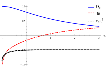
Figure 1: The behaviors of $\Omega_{B}$ (solid line), the deceleration parameter $q_{B}$ (dashed line) and squared speed of sound $v_{sB}^{2}$ (dotted line) in term of $z$ with $\gamma=12\cdot 9$ for type B modified Newtonian model.

II.3 Type C

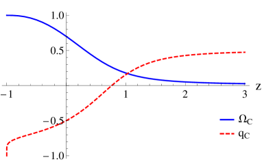
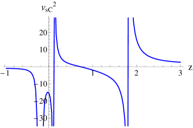
Figure 2: The behaviors of $\Omega_{C}$, $q_{C}$ and $v_{sC}^{2}$ in term of $z$ with $\gamma=108\cdot 843537$ and $\beta=0\cdot 007696$

Now, we focus on the third model obtained by using the second potential in (2). The third relation in (6) can be rewritten as

$$3H^{2}=8\pi G\left(\rho+\rho_{C}\right),$$ (15)

where $\rho_{C}=3\beta H^{2}e^{-\frac{\alpha}{H}}/8\pi G\left(1+\beta e^{-\frac{\alpha}{H}}\right)$. Indeed, we stored the effects of deviation from the Newtonian potential into $\rho_{C}$. Again, we consider a dust source nc4 satisfying ordinary energy-momentum conservation law ($\dot{\rho}_{C}=-3H\rho_{C}$). Thus, if an unknown pressure $p_{C}$ is attributed to the hypothetical fluid with energy density $\rho_{C}$, then we should have

$$\dot{\rho}_{C}+3H(\rho_{C}+p_{C})=0.$$ (16)

Now, combining the above relations with each other, one receives

$$3H^{2}+2\dot{H}=-8\pi Gp_{C},$$ (17)

$$\dot{H}=-4\pi G(\rho+\rho_{C}+p_{C}),$$ (18)

in which

$$p_{C}=-(\frac{\dot{\rho}_{C}}{3H}+\rho_{C})=$$

$$-\frac{\rho_{C}}{3}\left[\frac{\dot{H}}{H^{2}}\left(2+\frac{\alpha}{H}\left(1+\frac{8\pi G}{3}\rho_{C}\right)\right)+3\right].$$ (19)

Eq. (19) shows that $p_{C}\rightarrow-\rho_{C}$ whenever $\dot{H}\rightarrow 0$. It is also remarkable to note that, even without assuming Eq. (16), one can obtain Eq. (17) and the second line of Eq. (19) by combining the time derivative of Eq. (15) with itself and using this fact that the $\rho$ source is pressureless. In summary, we found out that the effects of deviation from the Newtonian potential can be simulated as a hypothetical fluid with energy density $\rho_{C}$ and pressure $p_{C}$. The density parameter of this fluid can be calculated as

$$\Omega_{C}=\frac{8\pi G\rho_{C}}{3H^{2}}=\frac{\beta e^{-\frac{\alpha}{H}}}{1+\beta e^{-\frac{\alpha}{H}}}.$$ (20)

The deceleration and total state parameters of the model can also be obtained by using $q_{C}=-1+(1+z)(dH(z)/dz)/H(z)$ and $\omega_{C}\equiv p_{C}/\left(\rho_{C}+\rho\right)$, respectively. Bearing the $\rho=\rho_{0}(1+z)^{3}$ in mind and combining the above equation with the corresponding Friedmann equation (15), we easily reach

$$z(\Omega_{C})=\left(\frac{\gamma\left(1-\Omega_{C}\right)}{\ln^{2}\left(\frac{\beta\left(1-\Omega_{C}\right)}{\Omega_{C}}\right)}\right)^{1/3}-1.$$ (21)

Eq. (21) implies that $z\geq-1$ for $\Omega_{C}\leq 1$. Calculations for the total state and deceleration parameters also lead to $\omega_{C}=\frac{2}{3}(q_{C}-\frac{1}{2})$ and

$$q_{C}=\frac{1-\Omega_{C}\ln\left(\frac{\Omega_{C}}{\beta(1-\Omega_{C})}\right)}{2+\Omega_{C}\ln\left(\frac{\Omega_{C}}{\beta(1-\Omega_{C})}\right)}.$$ (22)

These results clearly show that $q_{C},\omega_{C}\rightarrow-1$ as $\Omega_{C}\rightarrow 1$ (or equally $z\rightarrow-1$) and also $q_{C}\rightarrow\frac{1}{2}$ and $\omega_{C}\rightarrow 0$ as $\Omega_{C}\rightarrow 0$ (or equally $z\gg 1$).

In Fig. (2), we depict the behaviors of $\Omega_{C}$ and $q_{C}$ with respect to $z$ by choosing suitable constants so that the observation constraints are satisfied. It is worthwhile to note again that the value of $\alpha$ can be found by specifying the value of $\rho_{0}$ from observation and inserting it in $\alpha=\sqrt{8\pi\rho_{0}G\gamma/3}$ (see below Eq. (9)). In Fig. (2), we have plotted the behavior of $v_{sC}^{2}$ given by

$$v_{sC}^{2}=\frac{dp_{C}}{d\rho_{C}}=\frac{dp_{C}/dH}{d\rho_{C}/dH}.$$ (23)

Since the expression for $v_{sC}^{2}$ is too long, we have omitted it here. As one can see from Fig. (2), similar to type B and many of the dark energy models stab ; istab ; istab1 , Type C shows instability at present time too.

III Logarithmic Modification (type D) and Dark Energy

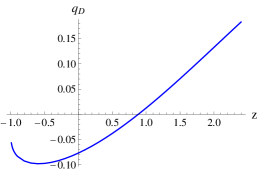
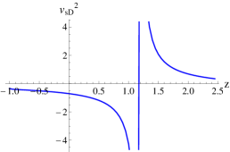
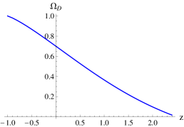
Figure 3: The behaviors of $\Omega_{D}$, $q_{D}$ and $v_{sD}^{2}$ in term of $z$ for $\eta=240$ and $\delta=122.5$ with $H\left(z=0\right)=67$ $km/\left(sMpc\right)$, $G=1$ and the current matter density parameter $\Omega\left(z=0\right)=0\cdot 3$.

Observations indicate that the universe is homogeneous and isotropic in the scales larger than $100$-Mpc. Moreover, the energy density of the dominant cosmic fluid ($\Lambda$) is approximately constant at the mentioned scales roos . In the Newtonian language, these results can be summarized as

$$\frac{1}{r^{2}}\left[\frac{d}{dr}\left(r^{2}\frac{d\phi}{dr}\right)\right]=4\pi G\Lambda,$$ (24)

which finally leads to

$$\phi(r)=\frac{2\pi G}{3}\Lambda r^{2}-\frac{C}{r},$$ (25)

for the modified Kepler potential of the energy source confined to the radius $r$. Here, $C$ is the integration constant, and in order to cover the Kepler potential ($-GM/r$) at the appropriate limit $\Lambda=0$, we should set $C=GM$, where $M$ is the mass content of system. Thus, the modified Newtonian potential felt by the test mass $m$ located at radius $r$ can be written as mz ; h1

$$V(r)\equiv m\phi(r)=\frac{2\pi Gm}{3}\Lambda r^{2}+V_{\mathrm{N}}(r).$$ (26)

It means that if we modify the Newtonian potential by a Hook term at the cosmic scales larger than $100$-Mpc, then the constant energy density obtained by the observations may be justified. Such potential can also be obtained in the non-local Newtonian gravity framework ynl . The light bending problem in the presence of the above potential has also been studied in Ref. mz . More studies on the above potential can be found in Ref. h1 and references therein.

Now, following the recipe used in this paper to find the Friedmann equations in the Newtonian framework, one can easily reach

$$H^{2}=\frac{8\pi G}{3}\left(\rho+\frac{\Lambda}{2}\right),$$ (27)

which has an additional coefficient $1/2$ for the $\Lambda$ term in comparison with the standard Friedmann equation in the presence of the cosmological constant. This additional coefficient will be disappeared if we modify the right hand side of Eq. (24) as $8\pi G\Lambda$. It means that the flux corresponding to the $\Lambda$ source is two times greater than those of the ordinary known sources. In this manner, the modified Kepler potential (25) finally takes the form

$$\phi(r)=\frac{4\pi G}{3}\Lambda r^{2}-\frac{GM}{r}.$$ (28)

Also, the corresponding Friedmann equations will be the same as those of the standard cosmology in the presence of the cosmological constant.

The Kepler potential modified by a logarithmic term which can describe the spiral galaxies rotation curves log1 ; log2 ; log3 is written as

$$\Phi(r)=-\frac{GM}{r}-\delta GM\ln(\eta r),$$ (29)

where $\delta$ and $\eta$ are some constants found by fitting the results with observations log1 ; log2 ; log3 . The potential (29) can be obtained by various ways (see ynl and references therein for details). Multiplying (29) by $m$, one can get the corresponding Newtonian potential felt by the test mass $m$ as

$$V(r)=V_{\mathrm{N}}(r)-\delta GmM\ln(\eta r),\text{ Type D}$$ (30)

in accordance with the results of the non-local Newtonian gravity ynl . Calculations for the cosmological equations corresponding to this potential lead to

$$3H^{2}=8\pi G\left(\rho+\rho_{D}\right),$$ (31)

where the energy density of the pressureless source is $\rho=\rho_{0}(1+z)^{3}$ and

$$\rho_{D}=\frac{3H^{2}}{8\pi G}\left(\frac{\delta\ln(\frac{H}{\eta})}{\delta\ln(\frac{H}{\eta})-H}\right).$$ (32)

One could also obtain

$$3H^{2}+2\dot{H}=-8\pi Gp_{D},$$

where $p_{D}=-\dot{\rho}_{D}/3H-\rho_{D}$ is a pressure originated from the logarithmic term. Hence, the density parameter is $\Omega_{D}=\delta\ln\left(\frac{H}{\eta}\right)/\left(\delta\ln\left(\frac{H}{\eta}\right)-H\right)$. Clearly, whenever $\delta>0$, we have $\Omega_{D}\rightarrow 0$ ($\Omega_{D}\rightarrow 1$) for $H\rightarrow\eta$ ($H\rightarrow 0$).

In Fig. (3), $\Omega_{D}$ and $q_{D}$ have been plotted with respect to $z$. We have not presented the explicit form of $q_{D}=-1+(1+z)(dH(z)/dz)/H(z)$ here since it is too long. Fig. (3) shows that $q_{D}\rightarrow\frac{1}{2}$ when $z\rightarrow z_{\eta}$, where $z_{\eta}$ denotes the redshift at which $H$ reaches its maximum possible value in this model, and hence, the value of $H$ at the beginning of the matter dominated era is a proper candidate for this maximum. Finally, we should note that since the total state parameter of type D is defined as $\omega_{D}\equiv p_{D}/\left(\rho+\rho_{D}\right)=\frac{2}{3}(q_{D}-\frac{1}{2})$, it is obvious that $\omega_{D}$ also exhibits satisfactory behaviors. $v_{sD}^{2}=dp_{D}/d\rho_{D}$ has been plotted in Fig. (3). It is apparent that none of the obtained models are stable for $z<0\cdot 1$.

IV Concluding remarks

Considering various modified Newtonian potentials, the Hubble law and the classical total energy of a test mass located at the edge of the universe, we could obtain some modified forms of the Friedmann equations. In this formalism, it has been obtained that some corrections to the Newtonian potential may model the current accelerated universe, and hence, dark energy. The interesting point is the ability of some of these corrected potentials in describing the spiral galaxies rotation curves. The latter fact signals that dark matter and dark energy may have some common origins and aspects dara . In fact, since all of the obtained models address an accelerated universe, one may conclude that the dark sides of cosmos may have at least some common roots. Consequently, from this standpoint, a more complete modified Newtonian potential may model the dark sides of cosmos simultaneously.

References

- (1) R. I. Ivanov, E. M. Prodanov, in Prof. G. Manev’s Legacy in Contemporary Aspects of Astronomy, Theoretical and Gravitational Physics, eds. V. Gerdjikov, M. Tsvetkov, Heron Press Ltd. Sofia, Articles. 102 (2005).
- (2) S. Kirk, I. Haranas, I. Gkigkitzis, Astrophys. Space. Sci. 344, 313 (2013).
- (3) F. Diacu, V. Mioc, C. Stoica, Nonlinear Anal. 41, 1029 (2000).
- (4) M. C. Anisiu, I. Szücs-Csillik, Astrophys. Space. Sci. 361, 382 (2016).
- (5) J. J. Rawal, J. V. Narlikar, J. Astrophys. Astron. 3, 393 (1982).
- (6) J. V. Narlikar, T. Padmanabhan, J. Astrophys. Astr. 6, 171 (1985).
- (7) I. V. Artemova, G. Bjoernsson, I. D. Novikov, Astrophys. J. 461, 565 (1996).
- (8) P. Fleury, Phys. Rev. D 95, 124009 (2017).
- (9) E. Fischbach, D. Sudarsky, A. Szafer, C. Talmadge, S. H. Aronson, Phys. Rev. Lett. 56, 3 (1986).
- (10) E. Fischbach, C. L. Talmadge, The Search for Non-Newtonian Gravity (Springer, New York 1999).
- (11) J. C. DÓlivo, M. P. Ryan Jr. Class. Quantum. Grav. 4, L 13 (1987).
- (12) C. R. Jamell, R. S. Decca, Int. J. Mod. Phys: Conference Series. Vol. 3, 48 (2011).
- (13) G. L. Klimchitskaya, V. M. Mostepanenko, Grav. Cosm. 20, 3 (2014).
- (14) I. Baldes, T. Konstandin, G. Servant, JHEP. 12, 073 (2016).
- (15) M. Eingorn, Int. J. Mod. Phys. D 26, 1750121 (2017).
- (16) A. Stabile, G. Scelza, Phys. Rev. D 84, 124023 (2011).
- (17) D. Borka, P. Jovanovi, V. Borka Jovanovi, A. F. Zakharov, JCAP. 11, 050 (2013).
- (18) A. F. Zakharov, P. Jovanovic, D. Borka, V. B. Jovanovic, JCAP. 05, 045 (2016).
- (19) I. Haranas and I. Gkigkitzis, Astrophys. Space. Sci. 337, 693 (2012).
- (20) N. Mebarki, F. Khelili, EJTP 5 (19), 65 (2008).
- (21) A. V. Ursulov, T. V. Chuvasheva, Astronomy Reports, 61, 468 (2017).
- (22) Y. Hagihara, Celestial Mechanics (MIT Press 1972).
- (23) M. Roos, Introduction to Cosmology (John Wiley and Sons, UK, 2003).
- (24) H. Bondi, Cosmology, (Camb. Univ. Press, 1952).
- (25) N. E. J. Bjerrum–Bohr, J. F. Donoghue, Holstein, Phys. Rev. D 67, 084033 (2003).
- (26) E. A. Malne, Quart. J. Math, 5, 64 (1934).
- (27) W. H. MacCrea, E. A. Malne, Quart. J. Math, 5, 73 (1934).
- (28) W. H. MacCrea, Rep. Prog. Phys. 16, 321 (1953).
- (29) W. H. MacCrea, Nature. 175, 466 (1955).
- (30) F. J. Tipler, Mon. Not. R. Astron. Soc. 282, 206 (1996).
- (31) R. C. Nunes, H. Moradpour, E. M. Barboza. Jr, E. M. C. Abreu, J. A. Neto, Int. Jour. Geom. Meth. Mod. Phys. 15, 1850004 (2018).
- (32) S. Capozziello, A. Stabile, A. Troisi, Phys. Rev. D 76, 104019 (2007).
- (33) S. Capozziello, E. Piedipalumbo, C. Rubano, P. Scudellaro, A& A 505, 21 (2009).
- (34) N. R. Napolitano, S. Capozziello, A. J. Romanowsky, M. Capaccioli, C. Tortora, The Astrophysical Journal. 748, 87 (2012).
- (35) C. Chicone, B. Mashhoon, Class. Quantum Grav. 33, 075005 (2016).
- (36) J. E. Tohline, Ann. New York Acad. Sci. 422, 390 (1984).
- (37) J. C. Fabris, J. Pereira. Campos, Gen. Relativ. Gravit. 41, 93 (2009).
- (38) L. Chang et al., RAA. 14, 1301 (2014).
- (39) F. A. Abd El-Salam, S. E. Abd El-Bar, M. Rasem, S. Z. Alamri, Astrophys. Space. Sci. 350, 507 (2014).
- (40) C. Corda, Int. J. Mod. Phys. D 18, 2275 (2009).
- (41) C. Corda, Int. J. Mod. Phys. D 27, 1850060 (2018).
- (42) E. Chang-Young, D. Lee, JHEP 1404, 125 (2014).
- (43) M. Eune, W. Kim, Phys. Rev. D 88, 067303 (2013).
- (44) H. Ebadi, H. Moradpour, Int. J. Mod. Phys. D 24, 1550098 (2015).
- (45) Y. S. Myung, Phys. Lett. B 652, 223 (2007).
- (46) W. Yang, S. Pan, J. D. Barrow, Phys. Rev. D 97, 043529 (2018).
- (47) M. Tavayef, A. Sheykhi, K. Bamba and H. Moradpour, Phys. Lett. B. 781, 195 (2018).
- (48) H. Miraghaei, M. Nouri-Zonoz, Gen. Rel. Grav. 42, 2947 (2010).
- (49) L. Calder, O. Lahav, Astronomy & Geophysics, 49, 1.13 (2008).
- (50) F. Darabi, MNRAS, 433, 1729 (2013).