Soliton generation in optical fiber networks

Abstract

We consider the problem of soliton generation in branched optical fibers. A model based on the nonlinear Schrodinger equation on metric graphs is proposed. Number of generated solitons is computed for different branching topologies considering different initial pulse profiles. Experimental realization of the model is discussed.

I Introduction

Optical solitons attracted much attention due to their potential applications in optoelectronics and information technologies. The idea of using optical solitons as carriers of information in high-speed communication systems was first proposed in the pioneering paper by Hasegawa and Tappert Hasegawa . Later due to the advances made in fiber technology it became possible to realize optical solitons experimentally in different versions (bright, dark, etc) Fiber1 -Kivsharbook . This fact caused great interest to finding the soliton solutions of governing nonlinear wave equations, such as nonlinear Schödinger equations with different nonlinearities. An important problem in the context of optical solitons is the problem of soliton generation in optical media. Mathematically, such problem is reduced to the initial value (Cauchy) problem for nonlinear Schödinger equation, which allows to find soliton solution and number of generated solitons using given initial condition. For optical fibers such problem was studied in the Refs.Burzlaff -Zhong1 . In Burzlaff an effective method for finding number of solitons generated in optical fibers was proposed. Later, it was extended for some other initial conditions Kivshar . Strict mathematical treatment of soliton generation on a half line as initial-boundary-value problem was considered presented Fokas . Soliton generation in optical fibers for a dual-frequency input was studied in Panoiu . In Skryabin a theory of the generation of new spectral components in optical fibers pumped with a solitonic pulse and a weak continuous wave was proposed and the wave number matching conditions for this process was derived. In Nishizawa characteristics of wavelength-tunable femtosecond soliton pulse generation using optical fibers in a negative dispersion region are studied experimentally and theoretically using the extended nonlinear Schrödinger equation, in which the wavelength dependence of parameters is considered. A comprehensive analysis of the generation of optical solitons in a monomode optical fibre from a superposition of soliton-like optical pulses at different frequencies in Panoiu1 , where it is found that there exists a critical frequency separation above which wavelength-division multiplexing with solitons is feasible. Soliton generation and their instability are investigated in a system of two parallel-coupled fibers, with a pumped (active) nonlinear dispersive core and a lossy (passive) linear one in Malomed1 . A theory of the generation of new spectral components in optical fibers pumped with a solitonic pulse have been studied. Bright-gap-soliton generation in finite optical lattices was discussed in Carusotto . Despite the fact that certain progress is made on theoretical and experimental study of soliton generation in optical fibers, all the studies are restricted by considering long, unbranched fibers. However, branched fibers are more attractive from the viewpoint of practical applications, as in may cases information-communication systems use optical fiber networks. Modeling of soliton generation and dynamics in optical fiber networks requires solving of nonlinear Schödinger equation on metric graphs.
We note that soliton dynamics described by integrable nonlinear wave equations attracted much attention during past decade Zarif -Karim2018 . In Zarif nonlinear Schödinger equation on metric graphs is studied and condition for integrability is derived in the form of a sum rule for nonlinearity coefficients. In zar2011 such study is extended to Ablowitz-Laddik equation. Stationary Schödinger equation on metric graphs and standing wave soliton in networks are studied in Adami ; noja ; Karim2013 ; Adami16 ; Adami17 . Integrable sine-Gordon equation on metric graphs is studied in caputo14 ; Our1 ; Karim2018 . Linear and nonlinear systems of PDE on metric graphs are considered in Bolte ; KarimBdG ; KarimNLDE .

In this paper we consider the problem of soliton generation in branched optical fibers, or, optical fiber networks described in terms of the initial value problem for nonlinear Schödinger equation on metric graphs. For different given initial conditions, we derive number of solitons generated by considering different network topologies. Unlike linear optical fibers, pulse generation and soliton dynamics in fiber networks strongly depend on the topology of latter. Propagating in such network optical soliton undergo to scattering and transmission through the network branching points that may cause additional effects such as interaction of incoming and scattered solitons, radiation, collisions, etc. Therefore effective transmission of information through the optical fiber networks requires proper tuning both the system architecture and initial pulse profiles. Depending on which branch, or vertex the initial pulse located, the number of solitons and their dynamics can be different. This fact provides powerful tool for tuning of the optical fiber network architecture and optimization of signal and information transmission. This paper is organized as follows. In the next section we briefly recall treatment of the problem of soliton generation for linear (unbrached) optical fibers. In section III we give formulation of the problem and its solution for star branched (Y-junction) optical fibers. Section IV extends the study for other network topologies, modeled by loop and tree graphs. Section V presents some concluding remarks.

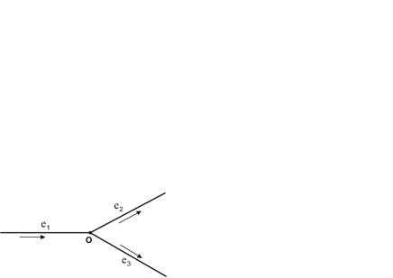
Figure 1: Basic star graph

II Soliton generation in linear optical fibers

Let us first, following the Refs.Burzlaff ; Kivshar , recall solution of the problem for linear, i.e. unbranched optical fibers. The governing equation for the pulse generation and evolution in optical fibers is the following nonlinear Schödinger equation

$$i\frac{\partial\psi}{\partial t}+\frac{1}{2}\frac{\partial^{2}\psi}{\partial x^{2}}+|\psi|^{2}\psi=0,$$ (1)

where $\psi$ is the normalized complex amplitude of the pulse envelope. The problem of soliton generation in optical fibers is reduced to the Cauchy problem for Eq.(1). Such problem can be solved, e.g., using inverse scattering method Burzlaff ; Kivshar ; Panoiu . In Burzlaff it was solved for the initial conditions given by $\psi(x,0)=-iq(x)$, with

$$q(x)=\begin{cases}0,&\text{for}\;\;\;|x|>\frac{1}{2}a\\ b,&\text{for}\;\;\;|x|\leq\frac{1}{2}a\end{cases}\quad\quad\quad b>0.$$ (2)

The evolution of the wave function upon generation of the soliton can be obtained via solving the following eigenvalue problem

$$Au=\lambda u,$$ (3)

where

$$A=\left(\begin{array}[]{cc}i\frac{d}{dx}&\psi(x,0)\\ -\psi^{*}(x,0)&-i\frac{d}{dx}\end{array}\right).$$ (4)

Figure 2: Initial pulse profile in the star branched optical fiber.

Each discrete eigenvalue $\lambda=\xi+i\eta$ with $L^{2}-$ integrable eigenfunction corresponds to the generated soliton with the amplitude $2\eta$ moving with the velocity $2\xi$. It was shown in Burzlaff that number of generated solitons is given by expression

$$N=<\frac{1}{2}+\frac{F}{\pi}>=<\frac{1}{2}+\frac{ab}{\pi}>,$$ (5)

where $F=\int_{-\infty}^{\infty}|\psi(x,0)|dx$ and $<...>$ denotes the integer smaller than the argument. Similar result for the number of solitons was obtained in the Ref.Burzlaff for the initial condition given by

$$q(x)=\beta\text{exp}(-\alpha|x|),\;\;\alpha,\beta>0.$$

Later, Kivshar considered the problem of soliton generation for super Gaussian initial pulse and showed that Eq.(5) is general formula for arbitrary initial profile Kivshar . More detailed treatment of the problem of soliton generation in optical fibers was presented in Panoiu . In particular, the authors of Panoiu analyzed scenarios for soliton generation in an ideal fiber for an input that consists of either two in-phase or out-of-phase solitonlike optical pulses at different frequencies by considering symmetric initial input pulse given by

$$\psi(x,0)=\text{sech}(x)[e^{i\omega x}+e^{-i\omega x}],$$

and asymmetric pulse given by

$$\psi(x,0)=i\text{sech}(x)[e^{i\omega x}-e^{-i\omega x}]$$

with the soliton solutions, respectively given as

$$\psi(x,t)=\xi\eta e^{\phi(\frac{t}{2})}\frac{e^{i\xi x}\cosh\left[\eta(x+\xi t)+i\varphi\right]+e^{-i\xi x}\cosh\left[\eta(x-\xi t)-i\varphi\right]}{\xi^{2}\cosh\eta(x+\xi t)\cosh\eta(x-\xi t)+\eta^{2}\sin\xi(x+i\eta t)\sin\xi(x-i\eta t)},$$

and

$$\psi(x,t)=-i\xi\eta e^{\phi(\frac{t}{2})}\frac{e^{i\xi x}\cosh\left[\eta(x+\xi t)+i\varphi\right]-e^{-i\xi x}\cosh\left[\eta(x-\xi t)-i\varphi\right]}{\xi^{2}\cosh\eta(x+\xi t)\cosh\eta(x-\xi t)+\eta^{2}\cos\xi(x+i\eta t)\cos\xi(x-i\eta t)},$$ (6)

where $\phi(t)=-i(\xi^{2}-\eta^{2})t+\alpha,\,\alpha=\ln|\lambda_{0}|,\,\tan\varphi=\frac{\eta}{\xi}$.

In the next section we extend these studies to the case of branched optical fibers, i.e. fiber networks.

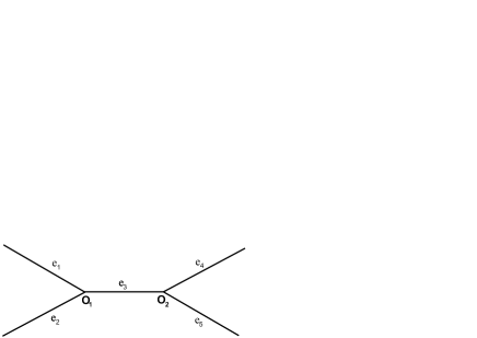
Figure 3: Sketch for the H-graph

III Description of the model for Star shaped network

Soliton dynamics in networks has attracted much attention during past decade. Convenient approach to describe such system is modeling in terms of nonlinear wave equation on a metric graph. The early treatment of the nonlinear Schrodinger equation on metric graphs dates back to the Ref. Zarif , where soliton solutions of the NLSE on metric graphs was obtained and integrability of the problem under certain constraints was shown by proving the existence of an infinite number of conserving quantities.

Here we briefly recall the problem of NLSE in metric star graph following the Ref. Zarif . Consider the star graph with three bonds $e_{j}$ (see, Fig. 1), for which a coordinate $x_{j}$ is assigned. Choosing the origin of coordinates at the vertex, 0 for bond $e_{1}$ we put $x_{1}\in(-\infty,0]$ and for $e_{2,3}$ we fix $x_{2,3}\in[0,+\infty)$. In what follows, we use the shorthand notation $\Psi_{j}(x)$ for $\Psi_{j}(x_{j})$ where $x$ is the coordinate on the bond $j$ to which the component $\Psi_{j}$ refers. The nonlinear Schrödinger equation on each bond $e_{j}$ of such graph can be written as Zarif

$$i\frac{\partial\psi_{j}}{\partial t}+\frac{\partial^{2}\psi_{j}}{\partial x^{2}}+\beta_{j}|\psi_{j}|^{2}\psi_{j}=0.$$ (7)

To solve Eq. (7) one needs to impose the boundary conditions at the branching point. This can be derived from the fundamental physical laws, such as norm and energy conservation, which are given as Zarif

$$\frac{dN}{dt}=0,\quad\frac{dE}{dt}=0,$$ (8)

where

$$N(t)=\int\limits_{-\infty}^{0}|\psi_{1}|^{2}\,dx+\int\limits_{0}^{\infty}|\psi_{2}|^{2}\,dx+\int\limits_{0}^{\infty}|\psi_{3}|^{2}\,dx$$

and

$$E=E_{1}+E_{2}+E_{3},$$

with

$$E_{k}=\int\limits_{e_{k}}\biggl{[}\left|\frac{\partial\psi_{k}}{\partial x}\right|^{2}-\frac{\beta_{k}}{2}|\psi_{k}|^{4}\biggr{]}\,dx.$$

As it was shown in the Ref. Zarif , the conservation laws Eq. (8) lead to the following vertex conditions

$$\sqrt{\beta_{1}}\psi_{1}(0,t)=\sqrt{\beta_{2}}\psi_{2}(0,t)=\sqrt{\beta_{3}}\psi_{3}(0,t),$$ (9)

and generalized Kirchhoff rules

$$\frac{1}{\sqrt{\beta_{1}}}\frac{d\psi_{1}}{dx}|_{x=0}=\frac{1}{\sqrt{\beta_{2}}}\frac{d\psi_{2}}{dx}|_{x=0}+\frac{1}{\sqrt{\beta_{3}}}\frac{d\psi_{3}}{dx}|_{x=0},$$ (10)

where $\beta_{j}$ are nonzero real constants. The asymptotic conditions for Eq. (1) are imposed as

$$\lim_{|x|\to+\infty}\psi_{j}=0.$$ (11)

The single soliton solutions of Eq. (1) fulfilling the vertex boundary conditions (9), (10) and the asymptotic condition, (11) can be written as Zarif

$$\psi_{j}(x,t)=a\,\sqrt{\frac{2}{\beta_{j}}}\,\frac{\exp\bigl{[}i\frac{vx}{2}-i(\frac{v^{2}}{4}-a^{2})t\bigr{]}}{\cosh[a(x-l-vt)]},$$ (12)

where the parameters $\beta_{j}$ fulfill the sum rule Zarif

$$\frac{1}{\beta_{1}}=\frac{1}{\beta_{2}}+\frac{1}{\beta_{3}}.$$ (13)

Here $v$, $l$ and $a$ are bond-independent parameters characterizing velocity, initial center of mass and amplitude of a soliton, respectively.

Consider branched optical fiber having the form of the Y-junction. Such system can be considered as basic star graph presented in Fig. 1. Then the problem of generation of soliton and its propagation can be modeled in terms of the Cauchy problem for nonlinear Schödinger equation on a basic star graph, which is given by Eq.(7) for which the following initial condition is imposed:

$$\psi_{j}(x,0)=-i\sqrt{\frac{2}{\beta_{j}}}q_{j}(x,).$$

Here $\psi_{j}$ is the normalized complex amplitude of the pulse envelope on $j$th bond (branch) of the graph and $q_{j}(x)$ is the initial profile of the amplitude. To solve this equation, one needs to impose the boundary conditions at the branching point (vertex) of the graph and determine the asymptotic of the wave function at the branch ends. These can be written in the form of Eqs. (9), (10) and (11).

Figure 4: Initial pulse profile on the optical fiber H-shaped network

Here we consider the problem of soliton generation for Y-junction of the optical fiber for the initial pulse profile given as (see, Fig. 1)

$$q_{1}(x)=\begin{cases}0,&x<-\frac{1}{2}a\\ b,&-\frac{1}{2}a\leq x\leq 0\end{cases}$$ (14)

$$q_{2,3}=\begin{cases}0,&x>\frac{1}{2}a\\ b,&0\leq x\leq\frac{1}{2}a\end{cases}$$ (15)

Such initial profile implies that soliton is generated around the branching point on each branch. Using the same method as that for linear optical fiber, we can compute the number of generated solitons, $N$ for such profile:

$$N=\left<\frac{1}{2}+\frac{F}{\pi}\right>,$$ (16)

where

$$F=\sum_{j=1}^{3}\int_{e_{j}}|\psi_{j}(x,0)|dx=\frac{ab}{2}\left[\sqrt{\frac{2}{\beta_{1}}}+\sqrt{\frac{2}{\beta_{2}}}+\sqrt{\frac{2}{\beta_{3}}}\right].$$ (17)

We assume that the sum rule is (13) is fulfilled, i.e. the problem is integrable. Difference between Eqs.(5) and (16) comes from the constant factor

$$(\sqrt{2\beta_{1}^{-1}}+\sqrt{2\beta_{2}^{-1}}+\sqrt{2\beta_{3}^{-1}}).$$

This allows tuning the soliton number and dynamics using different choices of the set $\beta_{j},\;(j=1,2,3).$ In addition, for simplicity, the above initial pulse profiles in Eqs.(14) and (15) are given at the vertex and have the same widths, $a$ and heights, $b$. However, in general case one can choose different widths and heights for different bonds. This also provides additional tool for tuning of the soliton number and dynamics.

Another initial pulse profile, for which the soliton number and solutions in a Y-junction fiber can be explicitly obtained is given by

$$\psi_{j}(x,0)=\sqrt{\frac{2}{\beta_{j}}}\text{sech}(x)\left[e^{i\left(\omega x+\frac{\theta}{2}\right)}+e^{-i\left(\omega x+\frac{\theta}{2}\right)}\right],$$ (18)

where $2\omega$ and $\theta$ are the frequency detuning and the phase difference between the two solitons, correspondingly. The two-soliton solution of the problem given by Eqs. (7), (9) and (10)can be written as

$$\psi_{j}(x,t)=\sqrt{\frac{2}{\beta_{j}}}\xi\eta e^{\phi(\frac{t}{2})}\frac{e^{i\xi x}\cosh\left[\eta(x+\xi t)+i\varphi\right]+e^{-i\xi x}\cosh\left[\eta(x-\xi t)-i\varphi\right]}{\xi^{2}\cosh\eta(x+\xi t)\cosh\eta(x-\xi t)+\eta^{2}\sin\xi(x+i\eta t)\sin\xi(x-i\eta t)},$$ (19)

which is valid under the constraint:

$$\frac{1}{\beta_{1}}=\frac{1}{\beta_{2}}+\frac{1}{\beta_{3}},$$ (20)

Corresponding soliton number is given by Eq.(16), where the quantity $F$ can be written as

$$F=2\pi\left(\sqrt{\frac{2}{\beta_{1}}}+\sqrt{\frac{2}{\beta_{2}}}+\sqrt{\frac{2}{\beta_{3}}}\right)\text{sech}\left(\frac{\pi\omega}{2}\right)\cos\left(\frac{\theta}{2}\right)$$

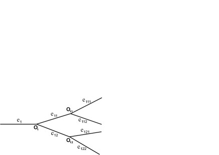
Figure 5: Sketch for tree graph

IV Other network topologies

The above treatment of the problem for soliton generation in optical fiber networks can be extended to the case of more complicated topologies. Here we demonstrate this for so-called $H-$graph and tree graph. For H-graph, presented in Fig.3 the coordinates are defines as $x_{1,2}\in(-\infty;0],\,x_{3}\in[0;L],\,x_{4,5}\in[0;+\infty),$ where $L$ is the length of bond $e_{3}$, i.e. the distance between two vertices.

For NLS equation (7) and the vertex boundary conditions given by

$$\sqrt{\beta_{1}}\psi_{1}(0,t)=\sqrt{\beta_{2}}\psi_{2}(0,t)=\sqrt{\beta_{3}}\psi_{3}(0,t),$$

$$\sqrt{\beta_{3}}\psi_{3}(L,t)=\sqrt{\beta_{4}}\psi_{4}(0,t)=\sqrt{\beta_{5}}\psi_{5}(0,t),$$ (21)

$$\frac{1}{\sqrt{\beta_{1}}}\frac{d\psi_{1}}{dx}|_{x=0}+\frac{1}{\sqrt{\beta_{2}}}\frac{d\psi_{2}}{dx}|_{x=0}=\frac{1}{\sqrt{\beta_{3}}}\frac{d\psi_{3}}{dx}|_{x=0},$$

$$\frac{1}{\sqrt{\beta_{3}}}\frac{d\psi_{3}}{dx}|_{x=L}=\frac{1}{\sqrt{\beta_{4}}}\frac{d\psi_{4}}{dx}|_{x=0}+\frac{1}{\sqrt{\beta_{5}}}\frac{d\psi_{5}}{dx}|_{x=0}.$$ (22)

We consider the following initial conditions:

$$\psi_{j}(x,0)=-i\sqrt{\frac{2}{\beta_{j}}}q_{j}(x)$$

where the initial pulse profiles are given by (see, Fig.4)

$$q_{1,2}(x)=\begin{cases}0,&-\infty<x<-\frac{1}{2}a\\ b_{1},&-\frac{1}{2}a\leq x\leq 0\end{cases}$$ (23)

$$q_{3}(x)=\begin{cases}b_{1},&0\leq x\leq\frac{1}{2}a\\ 0,&\frac{1}{2}a<x<L-\frac{1}{2}a\\ b_{2},&L-\frac{1}{2}a\leq x\leq L\end{cases}$$ (24)

$$q_{4,5}(x)=\begin{cases}b_{2},&0\leq x\leq\frac{1}{2}a\\ 0,&\frac{1}{2}a<x<\infty\end{cases}$$ (25)

Figure 6: Initial pulse profile on the tree-shaped optical fiber network

Then the number of generated optical solitons in such system we have explicit expression:

$$N=\left<\frac{1}{2}+\frac{F_{1}+F_{2}}{\pi}\right>,$$ (26)

where

$$F_{1}=\frac{ab_{1}}{2}\left[\sqrt{\frac{2}{\beta_{1}}}+\sqrt{\frac{2}{\beta_{2}}}+\sqrt{\frac{2}{\beta_{3}}}\right],$$ (27)

and

$$F_{2}=\frac{ab_{2}}{2}\left[\sqrt{\frac{2}{\beta_{3}}}+\sqrt{\frac{2}{\beta_{4}}}+\sqrt{\frac{2}{\beta_{5}}}\right].$$ (28)

Similarly, one can find number of generated solitons for the tree graph, presented in Fig. 6. The vertex boundary conditions for such graph are given by

$$\sqrt{\beta_{1}}\psi_{1}(0,t)=\sqrt{\beta_{2}}\psi_{2}(0,t)=\sqrt{\beta_{3}}\psi_{3}(0,t),$$

$$\sqrt{\beta_{1i}}\psi_{1i}(L_{1i},t)=\sqrt{\beta_{1ij}}\psi_{1ij}(0,t),\,i,j=1,2,$$ (29)

and

$$\frac{1}{\sqrt{\beta_{1}}}\frac{d\psi_{1}}{dx}|_{x=0}=\frac{1}{\sqrt{\beta_{2}}}\frac{d\psi_{2}}{dx}|_{x=0}+\frac{1}{\sqrt{\beta_{3}}}\frac{d\psi_{3}}{dx}|_{x=0},$$

$$\frac{1}{\sqrt{\beta_{1i}}}\frac{d\psi_{1i}}{dx}|_{x=L_{1i}}=\frac{1}{\sqrt{\beta_{1i1}}}\frac{d\psi_{1i1}}{dx}|_{x=0}+\frac{1}{\sqrt{\beta_{1i2}}}\frac{d\psi_{1i2}}{dx}|_{x=0},\,i=1,2.$$ (30)

Furthermore, we choose the initial pulse profile at each vertex ($\psi_{e}(x,0)=-i\sqrt{\frac{2}{\beta_{e}}}q_{e}(x)$) in the forms

$$q_{1}(x)=\begin{cases}0,&-\infty<x<-\frac{1}{2}a\\ b_{1},&-\frac{1}{2}a\leq x\leq 0\end{cases}$$ (31)

$$q_{11}(x)=\begin{cases}b_{1},&0\leq x\leq\frac{1}{2}a\\ 0,&\frac{1}{2}a<x<L_{11}-\frac{1}{2}a\\ b_{2},&L_{11}-\frac{1}{2}a\leq x\leq L_{11}\end{cases}$$ (32)

$$q_{12}(x)=\begin{cases}b_{1},&0\leq x\leq\frac{1}{2}a\\ 0,&\frac{1}{2}a<x<L_{12}-\frac{1}{2}a\\ b_{3},&L_{12}-\frac{1}{2}a\leq x\leq L_{12}\end{cases}$$ (33)

$$q_{1ij}(x)=\begin{cases}b_{i+1},&0\leq x\leq\frac{1}{2}a\\ 0,&\frac{1}{2}a<x<\infty\end{cases}$$ (34)

where $i,j=1,2$, $L_{11}$ and $L_{12}$ are lengths of bonds $e_{11}$ and $e_{12}$ respectively.

Then for the generated soliton number we have

$$N=\left<\frac{1}{2}+\frac{F_{1}+F_{2}+F_{3}}{\pi}\right>,$$ (35)

where

$$F_{1}=\frac{ab_{1}}{2}\left[\sqrt{\frac{2}{\beta_{1}}}+\sqrt{\frac{2}{\beta_{11}}}+\sqrt{\frac{2}{\beta_{12}}}\right]$$ (36)

$$F_{2}=\frac{ab_{2}}{2}\left[\sqrt{\frac{2}{\beta_{11}}}+\sqrt{\frac{2}{\beta_{111}}}+\sqrt{\frac{2}{\beta_{112}}}\right]$$ (37)

$$F_{3}=\frac{ab_{3}}{2}\left[\sqrt{\frac{2}{\beta_{12}}}+\sqrt{\frac{2}{\beta_{121}}}+\sqrt{\frac{2}{\beta_{122}}}\right]$$ (38)

The number of parameters in Eq.(35) is much higher that in the case of star graph. This implies that tree-shaped optical fiber network provides more wider possibility for tuning the generated soliton number and their dynamics.

V Conclusions

In this paper we studied the problem of soliton generation in optical fiber networks using a model based NLS equation on metric graphs. Initial value (Cauchy) problem for NLS equation on metric graphs is solved for different graph topologies, such as star, tree and H-graphs. For branched optical fibers one can choose the initial pulse profile in different ways (e.g., at the vertex or branch, at given vertex or branch, with different shapes at different vertices). Therefore, unlike to linear (unbranched) fibers, soliton generation for optical fiber networks have richer dynamics and tools for manipulation by solitons numbers. The above method can be applied for different network topologies, provided a network has three and more semi-infinite outgoing branches. This allows to use our model for the problem of tunable soliton generation in optical fiber networks, which is of importance for practical applications in the areas, where optical fibers are used for information (signal) transfer.

VI Acknowledgements

This work is supported by the grant of the Ministry for Innovation Development of Uzbekistan (Ref. No. BF2-022).

References

- (1) Hasegawa A and Tappert F 1973 Appl. Phys. Lett. 23 142
- (2) Mollenauer L F, Stolen R H and Gordon J P 1980 Phys. Rev. Lett. 45 1095
- (3) Zakharov V E and Shabat A B 1972 Sov. Phys.-JETP 34 62
- (4) Bullough R K and Caudrey P J (ed) 1980 Solitons (Berlin: Springer)
- (5) Scott A C, Chu F Y F and McLaughlin D W 1973 Proc. IEEE 61 1443
- (6) Satsuma J and Yajima N 1974 Prog. Theor. Phys. Suppl. 55 284
- (7) Hasegawa A and Kodama Y 1981 Proc. IEEE 69 1145
- (8) J. R. Taylor (Ed.) Optical Solitons: Theory and Experiment. (Cambridge University Press, Cambridge, England, 1992).
- (9) A. Hasegawa and Y. Kodama, Solitons in Optical Communications (Oxford University Press, Oxford, 1995).
- (10) Y. Kivshar and G. Agrawal, Optical Solitons: From Fibers to Photonic Crystals (Elsevier Science, 2003).
- (11) T. Dauxois, M. Peyrard, Physics of Solitons (Cambridge University Press, Cambridge, 2006).
- (12) J Burzlaff J. Phys. A: Math. Gen. 21 561 (1988).
- (13) Yu. S Kivshar J. Phys. A: Math. Gen. 22 337 (1989) .
- (14) S. A. Gredeskul and Yu. S. Kivshar, Phys. Rev. Lett., 62 977 (1989).
- (15) A. S. Fokas and A. R. Its, Phys. Rev. Lett., 68 3117 (1992).
- (16) N- C. Panoiu et al, Phys. Rev. A, 60 4 (1999).
- (17) N. Nishizawa, R. Okamura and T. Goto, Japanese J, Appl. Phys., 38 1 (1999).
- (18) N-C. Panoiu, I. V. Mel’nikov, D. Mihalache, C. Etrich and F. Lederer, J. Opt. B, 4 R53 (2002).
- (19) D. V. Skryabin and A. V. Yulin, Phys. Rev. E, 72 016619 (2005).
- (20) R.Ganapathy, B. A. Malomed, K.Porsezian, Phys. Lett. A, 354 366 (2006).
- (21) I. Carusotto, D. Embriaco, G. C. La Rocca, Phys. Rev. A, 65 4 (2002).
- (22) Y. V. Kartoshev et al Optics Lett., 31 15 (2006)
- (23) S. V. Chernikov, and J. R. Taylor, Optics Lett., 19 8 (1994)
- (24) X. Zhong, N. Yao, J. Sheng, K. Cheng, Opt. Laser Tech, 99, 1 (2018).
- (25) X. Zhong, B. Wu, K. Cheng, Optik, 162, 54 (2018).
- (26) Z.Sobirov, D.Matrasulov, K.Sabirov, S.Sawada, and K.Nakamura, Phys. Rev. E 81 , 066602 (2010).
- (27) Z. Sobirov, D. Matrasulov, S. Sawada, and K. Nakamura, Phys.Rev.E 84, 026609 (2011).
- (28) M. Stojanovic, A. Maluckova, Lj. Hadzievski, B.A. Malomed, Physica D 240 1489 (2011).
- (29) R.Adami, C.Cacciapuoti, D.Finco, D.Noja, Rev.Math.Phys, 23 4 (2011).,
- (30) K.K.Sabirov, Z.A.Sobirov, D.Babajanov, and D.U.Matrasulov, Phys.Lett. A, 377, 860 (2013).
- (31) D.Noja, Philos. Trans. R. Soc. A 372, 20130002 (2014).
- (32) J.-G.Caputo , D.Dutykh, Phys. Rev. E 90, 022912 (2014).
- (33) H.Uecker, D.Grieser, Z.Sobirov, D.Babajanov and D.Matrasulov, Phys. Rev. E 91, 023209 (2015).
- (34) D.Noja, D.Pelinovsky, and G.Shaikhova, Nonlinearity 28, 2343 (2015).
- (35) R.Adami, C.Cacciapuoti, D.Noja, J. Diff. Eq., 260 7397 (2016).
- (36) Z.Sobirov, D.Babajanov, D.Matrasulov, K.Nakamura, and H.Uecker, EPL 115 , 50002 (2016).
- (37) R Adami, E Serra, P Tilli, Commun. Math. Phys., 352, 387 (2017).
- (38) A. Kairzhan, D.E. Pelinovsky, J. Phys. A: Math. Theor. 51, 095203 (2018).
- (39) K.K.Sabirov, S. Rakhmanov, D. Matrasulov and H. Susanto, Phys.Lett. A, 382, 1092 (2018).
- (40) J.Bolte and J.Harrison, J. Phys. A: Math. Gen. 36 L433 (2003).
- (41) K.K.Sabirov, J.Yusupov, D. Jumanazarov, D. Matrasulov, Phys.Lett. A, 382, 2856 (2018).
- (42) K.K. Sabirov, D.B. Babajanov, D.U. Matrasulov and P.G. Kevrekidis, Arxiv:1701.05707.