Optimal Planar Electric Dipole Antennas

Abstract

Considerable time is often spent optimizing antennas to meet specific design metrics. Rarely, however, are the resulting antenna designs compared to rigorous physical bounds on those metrics. Here we study the performance of optimized planar meander line antennas with respect to such bounds. Results show that these simple structures meet the lower bound on radiation Q-factor (maximizing single resonance fractional bandwidth), but are far from reaching the associated physical bounds on efficiency. The relative performance of other canonical antenna designs is compared in similar ways, and the quantitative results are connected to intuitions from small antenna design, physical bounds, and matching network design.

I Introduction

Antenna parameters such as gain, Q-factor, and efficiency are limited by the geometry made available for a given design. Given bounds on these parameters under certain constraints, a designer can rapidly assess the feasibility of design requirements. This feasibility assumes the existence of an “optimal antenna” design which approaches the bounds on certain specified parameters. Synthesis of an optimal antenna is not a trivial task, and it remains to be demonstrated how an antenna designed to be optimal in one parameter (e.g., radiation Q-factor) performs relative to bounds on other parameters (e.g., efficiency). The goal of this paper is to discuss the synthesis and analysis of optimal antennas starting from classical antenna topologies.

Many strategies have been employed to optimize antennas. Heuristic optimization methods such as genetic algorithms [1, 2] and particle swarm optimization have the advantage of generating design geometries outside of the antenna designer’s usual catalog [3, 4, 5]. Such techniques have been used to design optimal antennas with radiation Q-factors very close to the physical bounds [6], though the resulting designs are computationally expensive to produce and offer only rough insight into guidelines for designing optimal antennas in volumes with arbitrary shapes and electrical size. Conversely, canonical antenna designs were shown [7, 8] to reach the lower bound on radiation Q-factor, but the question remains whether these designs represent optimal solutions over arbitrary electrical sizes and whether they are optimal in other parameters, e.g., radiation efficiency and input impedance. The cost of matching an optimal antenna design to arbitrary impedances is also unclear, regardless if matching is performed on the antenna itself or through external networks.

In this paper we study whether there exists a simple “recipe” for an optimal planar antenna (Throughout this paper, the term planar means to lie in a plane.) with respect to radiation Q-factor and radiation efficiency. In doing so, we ask whether, when prescribed with some form factor and electrical size, a simple design can be readily employed to achieve an antenna whose properties are sufficiently close to their bounds. The strategy adopted here is to optimize parameterizations of canonical antenna geometries known for good behavior in certain parameters. The examples studied here give quantifiable results to this end, i.e., how to design certain kinds of optimal antennas.

Along the way, we address the crossover of optimality of antennas across different performance parameters, e.g., do minimum radiation Q-factor antennas have inherently high radiation efficiency? Also discussed are the impacts of certain constraints, particularly those related to an antenna’s input impedance, on optimized parameters.

We stress out that this work differs significantly from other works on antenna optimization through parametric, heuristic, or metaheuristic means which typically involves the iterative evaluation and modification of designs until a local optimum or design goal is reached. Here, instead, we focus on designing antenna performance with respect to physical bounds, which provide an absolute measure in judging the quality of the synthesized design.

II Minimum Radiation Q-factor of planar TM antennas

We begin by studying the synthesis of electrically small dipole-like (TM) antennas with minimal radiation Q-factor $Q_{\mathrm{rad}}$ (see Box II and Box II). This leads to increased impedance bandwidth, however, the lower bound on radiation Q-factor increases rapidly as an antenna design region becomes smaller (see Box II). Thus, obtaining low Q-factor $Q_{\mathrm{rad}}$ is a key objective and challenge in the design of electrically small antennas.

[t]

[t]

TABLE I: Lower bounds on radiation Q-factors and efficiency in the limit of electrical size $ka\to 0$ for a sphere, a cylindrical tube, a rectangle, a thin strip dipole and a square loop.

	$(ka)^{3}Q_{\mathrm{rad}}^{\mathrm{lb}}$	$(ka)^{3}Q_{\mathrm{rad}}^{\mathrm{lb,TM}}$	$(ka)^{4}\eta_{0}/R_{\mathrm{s}}\delta$
	1	$\displaystyle\frac{3}{2}$	3
	4.5	4.6	59
	4.3	5.2	42
	16	16	3400
	5.3	7.4	130

II-A Synthesis of meander line antennas

Drawing from the prevalence of meander line antennas in applications requiring electrically small planar antennas [40, 24], as well as previous work studying their optimality in radiation Q-factor [8], we focus on determining whether meander lines present a consistent, simple solution, to obtaining minimum radiation Q-factor at arbitrary frequencies within rectangular design regions. Here, and throughout Section III, we specify a rectangular design region of fixed aspect ratio ($L/W=2$). The impact of varying aspect ratios is demonstrated and discussed in Section II-B.

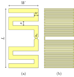
Figure 1: Panel (a) shows a parameterization of a meander line antenna used in this work. The antenna is fed via delta gap source along a horizontal line cutting the center of the meander line. The feeding region contains a taper between the feeding strip of width $d$ and the meander line of width $w$. The angle of the taper’s cut is $45^{\circ}$. Throughout the paper $d=\mathrm{min}\left(w,L/40\right)$ in order to keep the feeding region realistically narrow. Panel (b) shows a meander line antenna design “M1” from [8] within the parametrization used in this paper.

From the many possible meander line shapes (for example, rectangular, triangular, sinusoidal [40]) we have chosen the simple parametrization from Fig. 1. Thin wire versions of such antennas were previously shown to reach the lower bound on radiation Q-factor $Q_{\mathrm{rad}}$ for their corresponding rectangular design regions with electrical sizes near $ka=0.3$ [8]. Here, we use the parameterization in Fig. 1 to optimize the meander line antenna for resonance by requiring the magnitude of the normalized input reactance $X_{\mathrm{in}}/R_{\mathrm{in}}$ to be smaller than a specified tolerance, $\left|X_{\mathrm{in}}/R_{\mathrm{in}}\right|<10^{-3}$. This procedure is repeated at many frequencies (electrical sizes, values of $ka$) to obtain a set of antenna designs, each resonant at a specific frequency. The Q-factors $Q_{\mathrm{rad}}$ of the resulting designs were then calculated in AToM [41] and compared to the bounds discussed in Box II. The comparison is shown in Fig. 2. Note that the value of Q-factor $Q_{\mathrm{rad}}$ is just weakly dependent on dissipation factor (see Box III) provided that dissipation is not exceedingly high.

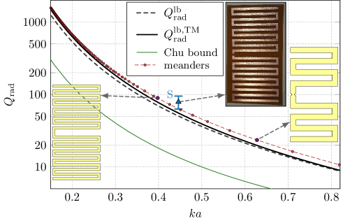
Figure 2: Radiation Q-factors of self-resonant meander line antennas simulated as made of PEC (markers) and the lower bound on radiation Q-factor (see Box II) corresponding to a rectangular region bounding the meander line. All meander lines are designed using the parameterization in Fig. 1 with $w/s=1$ and $L/W=2$. The defining parameters of all meandered dipoles are depicted in Fig. 3. A triangular marker with a corresponding error bar represents measured radiation Q-factor of selected meander line design.

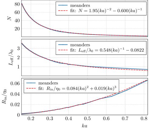
Figure 3: Design curves for the meander line antennas from Fig. 1. The panels show consecutively total number of meanders $N$, total length of the strip $L_{\mathrm{eff}}$ normalized to free-space wavelength, and input resistance $R_{\mathrm{in}}$ normalized to free-space impedance. In all cases $w/s=1$, $L/W=2$ and PEC are considered. One meander line ($N=1$) consists of two horizontal strips and vertical connections, i.e., meander line antennas in Fig. 1 have 3 and 20 meanders, respectively.

In order to verify the computed data in Fig. 2, an antenna design sample with $ka=0.42$ was scaled to $1.4$ GHz and fabricated on a $25\,\mu$m-thick Polyimide film with $17\,\mu$m-thick copper foil bonded by an $25\,\mu$m-thick acrylic adhesive ($\varepsilon_{\mathrm{r}}=4$). Thanks to the very thin profile of the substrate as compared to wavelength, the effect of dielectric can be neglected for a radiation Q-factor evaluation. The input impedance of the prototype was measured using a differential technique [42] and has been used to estimate the Q-factor via the $Q_{\mathrm{Z}}$ formula [12]. Radiation efficiency of the antenna was measured via a multiport near-field method [43] and was used to evaluate radiation Q-factor, and its confidence interval of width equal to two times the standard deviation, see triangular marker and corresponding error bar in Fig. 2.

Figure 2 illustrates that a simple parametrization, such as the one from Fig. 1, is able to closely approach the radiation Q-factor bound limited to TM radiation $Q_{\mathrm{rad}}^{\mathrm{lb,TM}}$ (see Box II) in the entire frequency range of electrically small antennas. From this, it is possible to conclude that a complex design (e.g., the parameterizations found in [44]) is not needed to reach the lower bound.

The absolute lower bound for radiation Q-factor $Q_{\mathrm{rad}}^{\mathrm{lb}}$ is unreachable by this meander line antenna since its planar geometry and single feed scenario does not allow for an efficient excitation of combined TE and TM radiation. This contrasts to three-dimensional (e.g., spherical) geometries [36, 25], where the dual mode behavior can be realized by a single feed network.

Parameters of the self-resonant designs from Fig. 2 are shown in Fig. 3. Design curves are fitted to the optimized parameters using a polynomial fit with good agreement. While some of the curves from Fig. 3 can be found in [40] for several parametrization, here all the designing curves are related back to Fig. 2 in which the Q-factor $Q_{\mathrm{rad}}$ is minimized. The presented data series can therefore be used for designing meandered dipoles approaching lower bounds on radiation Q-factor for TM antennas. It should, however, be noted that design curves from Fig. 3 depends on the used parametrization and are valid only for $L/W=2$ and $w/s\approx 1$.

II-B Varying aspect ratios

Meander line antennas, introduced in the previous section, are now studied for various $L/W$ and $w/s$ aspect ratios and compared against the fundamental bounds calculated for each form factor.

In all cases, the value of radiation Q-factor $Q_{\mathrm{rad}}$ is normalized with respect to the minimal TM radiation Q-factor. Generally, Fig. 4 shows that the minimal values can closely be approached for various $L/W$ aspect ratios. Slightly better performance is observed for higher $L/W$ ratios, however, at the cost of higher absolute bound on radiation Q-factor see top panel of Fig. 4.

With respect to the varying $w/s$ ratio, slightly better performance is observed for higher values, i.e., wider metallic strips. The differences become negligible for small values of $ka$, see Fig. 5. Notice, however, that this behavior is substantially changed when ohmic losses are introduced, mainly since the spatial proximity of out-of-phased currents degrades the radiation and enhance the ohmic losses [45].

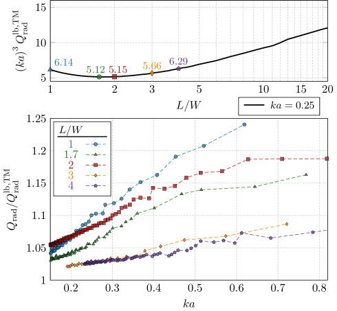
Figure 4: Radiation Q-factor performance of PEC self-resonant meandered dipoles from Fig. 2 for various $L/W$ aspect ratios. The radiation Q-factor is normalized to fundamental bound for a rectangular region which is shown in the top panel as a function of the aspect ratio. The minimum of the fundamental bound is found around ratio $L/W\approx 5/3$. Generally, the higher the $L/W$ ratio, the closer the meander lines are to the bound, however, at the cost of increasing absolute value of radiation Q-factor.

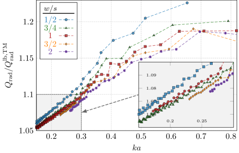
Figure 5: The same study as in Fig. 4 done for various ratios of meander line width $w$ to spacing $s$.

II-C The impact of impedance matching on Q-factor $Q_{\mathrm{rad}}$

The designs obtained above are all self resonant ($X_{\mathrm{in}}\approx 0$), but no constraint was placed on the value of the input resistance $R_{\mathrm{in}}$. In most practical cases, the objective antenna input resistance is not driven by any antenna consideration but is set by the radio frequency electronic equipment to be interfaced with a particular antenna. Transmission lines and active receivers based on Low Noise Amplifiers (LNA) often require matching to $50\,\,\Omega$. However, where devices with complex impedances are used, antenna resonance may not be ideal for conjugate matching and maximum power transfer. For example, a typical Power Amplifier (PA) output impedance is complex [46], with an input resistance lower than $50\,\,\Omega$ and an inductive (positive) reactive component. Similarly, passive RFID receivers based on Schottky diode rectifiers typically exhibit input resistances lower than $50\,\,\Omega$ and strong capacitive (negative) reactance [47]. Examples of nominal impedances $Z_{0}$ for these systems are listed in Table II.

TABLE II: Three impedances of practical significance for antenna system design.

System	Input impedance $Z_{0}$
Power amplifier (PA)	$15+\mathrm{j}50\,\Omega$
RFID chip (passive RX)	$20-\mathrm{j}200\,\Omega$
Low-noise amplifier (LNA)	$50\,\Omega$

Antennas may be designed to have input impedances which conjugate match a desired load. However, any of the designs shown in Fig. 2 can be conjugate matched to an arbitrary complex impedance $Z_{0}$ through an L-network consisting of two reactive components [48]. In many instances, the stored energies within these reactances will raise the radiation Q-factor of the system. To assess the cost of this form of simple matching, we select the design in Fig. 2 corresponding to self resonance at $ka=0.479$. A set of lossless networks was generated to conjugate match the antenna to arbitrary complex impedances and the matched radiation Q-factors were calculated. A typical frequency dependence of this cost is depicted in Fig. 6 while the dependence on matching impedance is depicted in Fig. 7. We observe that it is generally possible to transform the resonant antenna impedance to an arbitrary real value with minimal increase in radiation Q-factor, except when small resistance and high reactance is required. As expected, adding a reactive component to the real-valued (resonant) antenna impedance necessarily increases radiation Q-factor, though this increase is on the order of $30\%$ for the most extreme of the three test impedances (RFID) examined here. Additionally, Fig. 6 shows that it is often possible to move slightly away from the self-resonant frequency and lower the overall radiation Q-factor by a small amount. Nonetheless, the minimum radiation Q-factor of the matched antenna is, for practical values of the matching impedance, within the vicinity of the self-resonance of the antenna.

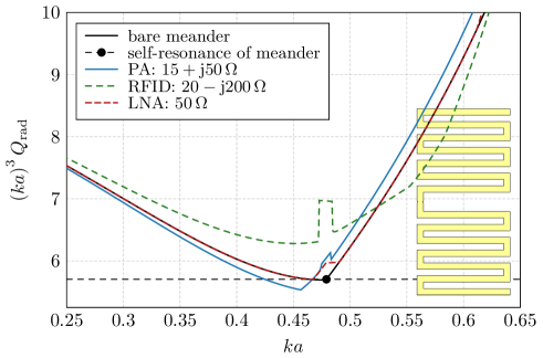
Figure 6: Matched radiation Q-factor of a selected meander line antenna for several impedance matching scenarios listed in Table II. Matching to each impedance is accomplished via a two-element reactive L-network, see inset in Fig. 7 for a schematic. In cases when several L-networks exist for a given matching impedance, the network with the lowest stored energy has been used. Abrupt jumps of the matched radiation Q-factor curves result from non-existence of matching by two inductances in certain frequency ranges. This double inductance matching is the most favorable scenario for a capacitive antenna.

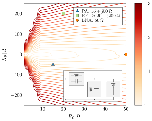
Figure 7: Matched radiation Q-factor of a selected meander line antenna for varying complex matching impedance normalized to radiation Q-factor of bare antenna. For each complex impedance, the meander line is conjugate matched at its self-resonance (circle mark in Fig. 6, $ka\approx 0.479$) using the lossless L-network matching circuit with lowest Q-factor. The markers denote the three impedances from Fig. 6 and Table II.

The importance of Q-factor is its relation to fractional bandwidth which is predicated on simple, single resonance behavior [12]. We demonstrate that the low variance in Q-factor corresponds to consistent realized bandwidth when L-networks are used to conjugate match an antenna to an arbitrary impedance. Figure 8 shows the power delivered $P_{\mathrm{del}}$ to the meander line antenna studied above using a matched source ($Z_{0}=R_{\mathrm{in}}$) as well as with L-networks designed to match the antenna to the three complex impedances of practical interest in Table II. In each case, a network tunes the antenna to the desired (possibly complex) impedance at its natural resonant frequency. The frequency profile of the mismatch factor [48, 49]

$$\tau=\frac{P_{\mathrm{del}}}{P_{\mathrm{cm}}}=\frac{4R^{\mathrm{m}}_{\mathrm{in}}R_{0}}{|Z_{\mathrm{in}}^{\mathrm{m}}+Z_{0}|^{2}}$$ (4)

is nearly identical in all four cases, in agreement with the predictions based on the relatively invariant Q-factor across these cases. Here, $Z_{\mathrm{in}}^{\mathrm{m}}$ is the antenna impedance including the tuning network, $P_{\mathrm{del}}$ is the power delivered to the antenna, and $P_{\mathrm{cm}}$ is the power delivered under a conjugate match condition. It is necessary to point out that we have assumed non-dispersive matching impedances, i.e., $\partial Z_{0}/\partial\omega=0$. In practice, the matching impedance may be dispersive within the band of interest, in which case the relation between Q-factor and bandwidth described in [12] ceases to be valid. However, inclusion of a dispersive load impedance may not necessarily cause major changes to the realized bandwidth due to the already heavily frequency-dependent nature of the impedance of high Q-factor antennas. Despite this simplification, when generating Fig. 8, lumped inductors and capacitors in each tuning network are modeled as frequency dependent impedances.

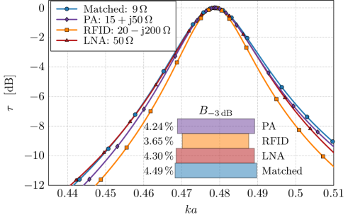
Figure 8: Frequency dependence of normalized power delivered $P_{\mathrm{del}}/P_{\mathrm{cm}}$ to the meander line studied in Figs. 6 and 7. The separate curves correspond to devices exhibiting the three practically relevant impedances from Table II and to a device with impedance corresponding to that of the meander line at its self-resonance (“Matched”). In each case, the antenna is conjugate matched using an L-network at its self resonant frequency, $ka\approx 0.479$. The $-3~{}\mathrm{dB}$ bandwidths $50\%$ power delivered bandwidths $B_{-3~{}\mathrm{dB}}$ for each scenario are also listed.

The results in Figs. 7 and 8 numerically suggest that there is little cost in bandwidth to match a self-resonant antenna to arbitrary impedances. However, further considerations reveal why it is of practical importance to design an antenna with a given impedance, rather than relying on this form of matching. First, the use of lumped components increases complexity and cost of an antenna system and the required component values for the L-networks described in this section may not be realizable. Second, lumped components made of any practical, lossy material (e.g., metallic inductors) increase the net loss in an antenna system while not adding any potential radiation mechanism. This guarantees a decrease in overall efficiency, particularly in high Q-factor antennas [50]. Additionally, tunability or the use of broadband multiple resonance matching may benefit from the design of an antenna with specific impedance characteristics, e.g., to increase the radiation resistance [51, 8].

III Radiation efficiency of Q-optimal antennas

The previous section demonstrated that meander line antennas are nearly optimal with respect to radiation Q-factor, including the cases when matching to realistic complex impedances is desired. This section studies how these antennas perform with respect to another critical antenna metric: radiation efficiency (see Box III). Specifically, we examine their performance with respect to radiation efficiency bounds (see Box III).

Before presenting the radiation efficiency of matched meander line antennas it is necessary to deal with losses in the matching circuit since, similarly to the case of Q-factor, any matching circuit with finite losses will worsen the overall efficiency of the antenna system. Throughout this section we will assume that all matching networks are composed of lossless capacitors and lossy inductors. The inductors are further assumed to be planar, made of the same material (metallic sheet, surface resistivity $R_{\mathrm{s}}$) as the antenna itself. Under such restrictions it is possible to estimate the loss added by a matching network quite precisely using data from Fig. 9, which shows the normalized reactance, $\left(10^{3}/ka_{L}\right)\left(R_{\mathrm{s}}/\eta_{0}\right)\left(X_{\mathrm{L}}/R_{\mathrm{L}}\right)$, of several spiral inductors as a function of their electrical size. Here $\eta_{0}$ denotes the free space impedance. The normalized reactance in Fig. 9 is independent on surface resistance $R_{s}$ and, at small electrical size, just weakly dependent on number of turns and frequency, consistent with classical relations for helical air-core inductors [52]. A conservative value $\left(10^{3}/ka_{\mathrm{L}}\right)\left(R_{\mathrm{s}}/\eta_{0}\right)\left(X_{\mathrm{L}}/R_{\mathrm{L}}\right)=66$ will be used in this section to determine losses of all inductors within the L-matching network, assuming further that inductors are always ten times smaller in electrical size than the antenna, i.e., $a_{L}=a/10$. This last assumption enforces the use of an electrically small, approximately lumped element, matching network.

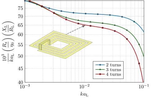
Figure 9: Normalized reactances of selected rectangular spiral inductors. The quantities $X_{\mathrm{L}}$, $R_{\mathrm{L}}$, and $R_{\mathrm{s}}$ denote input reactance, input resistance, and surface resistance, respectively. The radius $a_{\mathrm{L}}$ defines the smallest sphere circumscribing the inductor.

Lossy elements with the above mentioned specifications are used to match the meander studied in Figs. 6–8 to impedance $Z_{0}=50\,\Omega$ over a band of interest near the meander line’s self-resonant frequency. The resulting radiation Q-factor and efficiency (here presented in the form of dissipation factor, $\delta$) are depicted in Fig. 10 as functions of frequency (scaled as electrical size $ka$). The figure reiterates the previously-observed near-optimal performance of meander line antennas with respect to radiation Q-factor, but, surprisingly, shows a rather poor performance with respect to radiation efficiency. This metric is, at the self-resonance frequency of the antenna, almost one order of magnitude worse than the value of the physical bound (see Box III). Similarly to radiation Q-factor, dissipation factor reaches its minimum in the vicinity of the resonance frequency, at least in the case of realistic values of matching impedances used here.

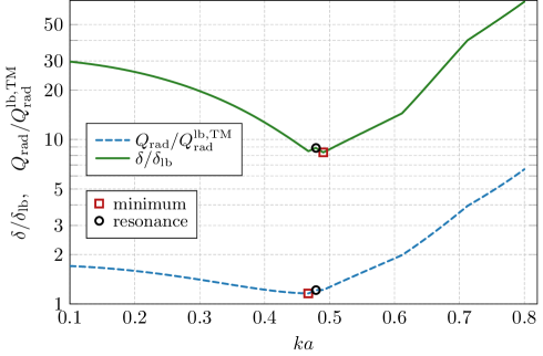
Figure 10: Normalized radiation Q-factor and normalized dissipation factor of a selected meander line antenna matched to $50\,\Omega$ over a range of frequencies (scaled here as electrical size $ka$). The self-resonance of the antenna ($ka=0.47$) is denoted on each trace with a circular marker while the minimum of each trace is also marked. The same data are also plotted as a curve parameterized by frequency in Fig. 11.

Within the used normalization of dissipation factor and radiation Q-factor, it is reasonable to represent the data from Fig. 10 as a two dimensional curve (radiation Q-factor vs. dissipation factor) parametrized by frequency, see Fig. 11. The figure also shows the Pareto front (represented by the black line) evaluated by the method from [53], which demonstrates the optimal trade-off between radiation Q-factor and dissipation factor for the given design geometry and frequency. The Pareto front has been evaluated at $ka=0.5$, but, due to the used normalization, it is almost independent of electrical size. The Pareto front was evaluated for a combination of TM and TE modes which, as normalized to the TM bound $Q_{\mathrm{rad}}^{\mathrm{lb,TM}}$, gives values lower than one. The reason for this particular normalization is that TM bounds represent meaningful limit of one-port planar antennas.

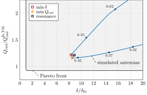
Figure 11: A two-dimensional view of the lower bounds on dissipation factor and radiation Q-factor. A black solid curve denotes the Pareto front describing the trade-off between these quantities and the corresponding feasible region (shaded). The data from Fig. 10 are drawn as a curve parameterized by frequency, with the relevant points in Fig. 10 being similarly marked. The circle markers along the curve representing the simulated antenna show the electrical size $ka$.

The two-dimensional plot in Fig. 11 represents a complete comparison of various antenna designs with respect to matched efficiency and matched radiation Q-factor. An example of such comparison is shown in Fig. 12, where the normalized and frequency-parameterized $Q$–$\delta$ curves are drawn for several small antenna designs within the same design specifications. Figure 12 clearly presents the superior performance in efficiency and Q-factor of simple meander line antennas shown in Fig. 1 with respect to other designs. It also shows that although there exist other meander lines which perform slightly better in radiation efficiency (Palmier pastry type, [54]) this improvement costs much in the radiation Q-factor. In conclusion, simple meander line antennas present the best trade-off between radiation Q-factor and dissipation factor from the depicted antennas when matching to real impedances is demanded. As in the previous section, we note that the use of more advanced matching topology (e.g., folding or impedance transformer) may benefit from alternative antenna designs.

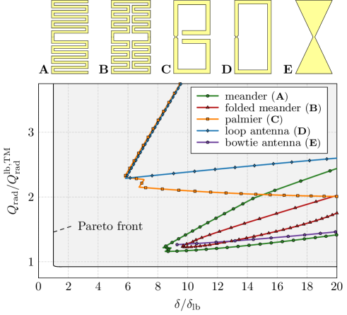
Figure 12: Two dimensional frequency parametrized plot representing the physical bound and several antennas. The matching impedance equals to $50\,\Omega$. The tip of each curve lies in the vicinity of resonance or anti-resonance of the antenna. The electrical sizes at the resonance or anti-resonance frequency are: A ($ka=0.48$, res.), B ($ka=0.85$, res.), C ($ka=0.50$, res.), D ($ka=0.59$, anti-res.), E (no resonance).

Figures 11 and 12 show that the considered antenna structures, which are close to optimal in radiation Q-factor, are far away from the efficiency bounds. This is puzzling since resonant modes optimal in radiation Q-factor and efficiency are similar in nature. However, there are important differences. Radiation Q-factor restricted to TM modes is minimized by separation of charges and inducing dipole like currents [38]. These modes can be tuned to resonance by inducing edge loops along the structure. TM efficiency, on the other hand, is minimized by inducing homogeneous currents [55]. These are similar in nature to the dipole like currents minimizing Q-factor, but the loop currents which minimize TE Q-factor and maximize TE efficiency are fundamentally different. Where low Q-factor loops tend to be confined towards the edges of the structure, high efficiency loops are spread across the whole area [53, Fig. 4]. Such loop currents are naturally restricted as an original simply connected object fully filling a prescribed bounding box is perforated, forcing the current distribution into more inhomogeneous forms. Thus, low Q-factor loops are tolerant of alterations to a structure whereas high efficiency loops are harshly disrupted.

In Fig. 13, the optimal resonant Q-factor and dissipation factor are plotted normalized to the corresponding bounds of a rectangular plate. Data for different shapes made by removing portions of the plate are shown. The currents on the structures in Fig. 13 have been calculated with current optimization without physical feeding. It is clear that removing metal does not greatly affect the achievable radiation Q-factor, at worst reducing it to the TM-only bound. However, when metal is removed from the plate the loss factor is significantly increased, especially for small electrical sizes. Thus, while optimal radiation Q-factor and radiation efficiency modes are fairly similar, removing design space has a much greater effect on the loss factor than the Q-factor in relation to the physical bounds. This can be seen in Fig. 13 where the loss factor of the optimal resonant currents is very high for the structures with slots in them. Consider the meander line antenna which has significantly higher loss factor at electrical sizes $ka<0.4$, here the loop modes are extremely disrupted, however, the Q-factor is hardly affected. The sharp change in the meander line’s loss at around $ka=0.6$ is due to its resonance, where it is possible to induce a resonant dipole mode on the structure. This example illustrates a fundamental challenge in designing efficient small resonant antennas: many of the strategies normally utilized to induce resonance, such as meandering, harshly limit the achievable efficiency.

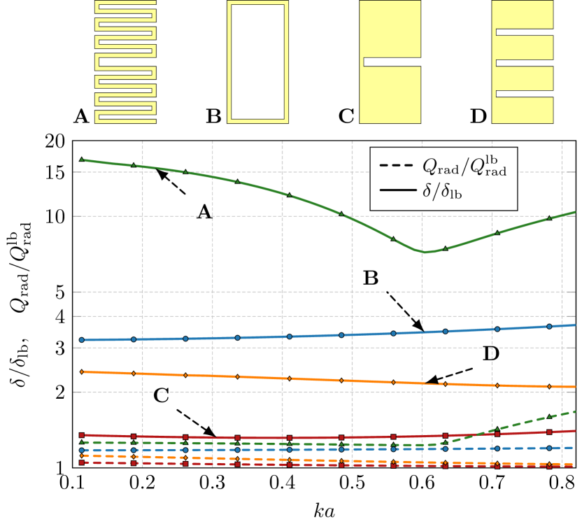
Figure 13: Illustration of how much different metrics deteriorate when a solid plate is permuted. The figure shows four generic shapes, a single slot, three slots, a meander line, and a loop. The ratio between optimal loss factor for different geometries and the optimal loss factor for the full plate are shown in solid lines. The ratio between the optimal mixed mode Q-factor for the same geometries and the optimal mixed mode Q-factor of the full plate are shown in dashed lines.

[t]

[t]

IV Antennas optimal in other parameters

Determining the best possible Q-factor can be formulated as a minimization problem. Therefore it is possible to add different or additional constraints to such an optimization. So far, in this paper, we have considered the constraints of efficiency and impedance matching. Another type of constraints are different kinds of field-shaping requirements of near and/or far-fields [62, 63]. For small antennas it is well known that the radiated far-field tends to resemble a dipole pattern, meander line antenna treated in this paper being no exception, see Fig. 14. However, with these types of Q-factor optimization procedures it is possible to determine the Q-factor cost, to have the antenna radiating with a certain front-to-back ratio or (super-) directivity in a given direction. These classes of bounds indicate that for a limited bandwidth cost it is possible to extend, e.g., the directivity beyond the traditional dipole pattern, see  [62, 63, 64, 65, 66, 67, 68, 69].

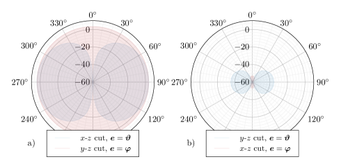
Figure 14: Directivity (in dB scale) with respect to an isotropic radiator of a meander line antenna depicted in Fig. 2 as the very right inset. Antenna is placed in $x$-$z$ plane, with a longer side aligned with $z$-direction.

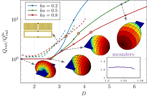
Figure 15: The cost in Q-factor for a desired directivity in a lossless 2:1 shaped antenna. The three line colors represent electrical sizes $ka=\left\{0.2,0.5,0.8\right\}$ and the radiation patterns correspond to the $ka=0.5$ case for the optimal current. All $Q$- vs $D$-values for the meander lines of Fig. 2 are represented in purple, and the relevant region is zoomed in the right bottom inset. Dashed curves show the results for an array composed of a meander line antenna element with one feed and a loop antenna element with two feeds.

To illustrate bounds on superdirectivity, Q-factor optimization for a given directivity described in [62, 63], was solved for a small antenna with length to width ratio of 2:1, infinitesimal thickness, and electrical sizes $ka\in\left\{0.2,0.5,0.8\right\}$. The bounds for low directivities are identical to the lower bound on the Q-factor, where the radiation pattern changes from that of an elliptically polarized dipole with $D\approx 1.5$ to that of a Huygens source with directivity just below $D=3$ and the main beam pointing in the direction of the longest side [21]. Higher directivities require quadrupole and higher order modes which increases the Q-factor rapidly [10]. The direction of the main beam changes from the longest side of the antenna to an endfire pattern along the shortest side at $Q_{\mathrm{rad}}/Q_{\mathrm{rad}}^{\mathrm{lb,TM}}\approx 3$ as indicated by circles in Fig. 15.

Much like bounds on other parameters (e.g., efficiency), it is an open problem if the directivity-constrained limits are reachable for all sizes and desired directivity, even under idealized lossless conditions. As a demonstration of one possible high directivity, low Q-factor design, a three port array composed of a meander line and a loop structure with optimized feeding is presented in relation to the bounds, see Fig. 15. However, high directivity for single port antennas remains, as of yet, far from the bound and new designs ideas that allow a high directivity with larger bandwidth are desired.

V Conclusion

The possibilities how to approach the fundamental bounds on selected antenna metrics were investigated. A planar region of rectangular form factor was considered. It was observed that the lower bound on Q-factor with radiation restricted to TM modes only is closely approached by a meander line antenna for a broad range of electrical sizes. The optimal design parameters were depicted and various aspect ratios of the bounding rectangle were studied together with selected ratios of the strip and slot widths. The simulated results were verified by a measurement of a fabricated prototype. The impedance matching and its impact on the Q-factor of the antenna was studied, concluding that the effect of the impedance matching on radiation Q-factor is minor and, in some cases, that matching the antenna slightly away from its self-resonance can even decrease its Q-factor. Radiation efficiency of the meander line antennas optimal in Q-factor was evaluated, taking into account ohmic losses dissipated in the matching circuit. It was observed that the radiation efficiency of the studied meander line antennas is far from an upper bound of a rectangular patch. Several other planar antennas were similarly evaluated against fundamental bounds yielding consistent conclusions: synthesizing antenna designs which approach the upper bound on radiation efficiency is more difficult than designing those which reach the lower bound on Q-factor. The reason was identified in the high sensitivity of radiation efficiency to the perturbation of ideal constant current density. Namely, when an initial structure fully filling the prescribed bounding box is perforated (as is done in a practical synthesis procedure), the performance of maximum efficiency current distributions drops much faster than that of a minimum Q-factor distribution. Finally, a Pareto-type bound between Q-factor and directivity has been calculated and compared to meander line antennas. An attempt has been made to find an antenna with reasonably low Q-factor and directivity higher than that of an electric dipole type antenna. Nevertheless, no planar antenna with one feed fulfilling these contradictory constraints was found. This task and its feasibility remains as a subject for ongoing research.

The fundamental bounds, i.e., the lower bounds on Q-factor, the upper bounds on radiation efficiency, the Pareto-optimality between Q-factor and efficiency, or Q-factor and directivity, were demonstrated to be powerful tools for judging the performance of the radiating devices. If the realistic designs are compared to the fundamental bounds, designer can assess how far from the optima the design is, therefore, if further improvement is needed. Furthermore, incremental progress in design improvement can be put into context by considering the remaining distance between an antenna’s realized performance and the fundamental bounds. It is the normalized ratio of the actual device’s performance to the fundamental bounds what reveals the real quality of the design.

References

- [1] Y. Rahmat-Samii and E. Michielssen, Eds., Electromagnetic Optimization by Genetic Algorithm. Wiley, 1999.
- [2] R. L. Haupt and D. H. Werner, Genetic Algorithms in Electromagnetics. Wiley-IEEE Press, 2007.
- [3] Y. Rahmat-Samii, J. M. Kovitz, and H. Rajagopalan, “Nature-inspired optimization techniques in communication antenna design,” Proc. IEEE, vol. 100, no. 7, pp. 2132–2144, July 2012.
- [4] G. C. Onwubolu and B. V. Babu, New Optimization Techniques in Engineering. Springer, 2004.
- [5] K. Deb, Multi-Objective Optimization using Evolutionary Algorithms. Wiley, 2001.
- [6] M. Cismasu and M. Gustafsson, “Antenna bandwidth optimization with single frequency simulation,” IEEE Trans. Antennas Propag., vol. 62, no. 3, pp. 1304–1311, 2014.
- [7] M. Gustafsson, C. Sohl, and G. Kristensson, “Illustrations of new physical bounds on linearly polarized antennas,” IEEE Trans. Antennas Propag., vol. 57, no. 5, pp. 1319–1327, May 2009.
- [8] S. R. Best, “Electrically small resonant planar antennas,” IEEE Antennas Propag. Mag., vol. 57, no. 3, pp. 38–47, June 2015.
- [9] 145-2013 – IEEE Standard for Definitions of Terms for Antennas, IEEE Std., March 2014.
- [10] L. J. Chu, “Physical limitations of omni-directional antennas,” J. Appl. Phys., vol. 19, pp. 1163–1175, 1948.
- [11] R. L. Fante, “Quality factor of general antennas,” IEEE Trans. Antennas Propag., vol. 17, no. 2, pp. 151–155, Mar. 1969.
- [12] A. D. Yaghjian and S. R. Best, “Impedance, bandwidth and Q of antennas,” IEEE Trans. Antennas Propag., vol. 53, no. 4, pp. 1298–1324, April 2005.
- [13] R. E. Collin and S. Rothschild, “Evaluation of antenna Q,” IEEE Trans. Antennas Propag., vol. 12, pp. 23–27, Jan. 1964.
- [14] R. F. Harrington and J. R. Mautz, “Control of radar scattering by reactive loading,” IEEE Trans. Antennas Propag., vol. 20, no. 4, pp. 446–454, 1972.
- [15] D. R. Rhodes, “Observable stored energies of electromagnetic systems,” Journal of the Franklin Institute, vol. 302, no. 3, pp. 225–237, 1976.
- [16] R. E. Collin, “Minimum Q of small antennas,” J. Electromagnet. Waves Appl., vol. 12, pp. 1369–1393, 1998.
- [17] G. A. E. Vandenbosch, “Reactive energies, impedance, and Q factor of radiating structures,” IEEE Trans. Antennas Propag., vol. 58, no. 4, pp. 1112–1127, Apr. 2010.
- [18] M. Gustafsson, M. Cismasu, and B. L. G. Jonsson, “Physical bounds and optimal currents on antennas,” IEEE Trans. Antennas Propag., vol. 60, no. 6, pp. 2672–2681, June 2012.
- [19] W. Geyi, Foundations of Applied Electrodynamics. John Wiley & Sons, 2011.
- [20] M. Gustafsson and B. L. G. Jonsson, “Stored electromagnetic energy and antenna Q,” Progress In Electromagnetics Research (PIER), vol. 150, pp. 13–27, 2015.
- [21] M. Capek, M. Gustafsson, and K. Schab, “Minimization of antenna quality factor,” IEEE Transactions on Antennas and Propagation, vol. 65, no. 8, pp. 4115–4123, 2017.
- [22] M. Gustafsson and B. L. G. Jonsson, “Antenna Q and stored energy expressed in the fields, currents, and input impedance,” IEEE Trans. Antennas Propag., vol. 63, no. 1, pp. 240–249, 2015.
- [23] K. Schab, L. Jelinek, M. Capek, C. Ehrenborg, D. Tayli, G. A. Vandenbosch, and M. Gustafsson, “Energy stored by radiating systems,” IEEE Access, vol. 6, pp. 10 553 – 10 568, 2018.
- [24] J. L. Volakis, C. Chen, and K. Fujimoto, Small Antennas: Miniaturization Techniques & Applications. McGraw-Hill, 2010.
- [25] H. L. Thal, “New radiation Q limits for spherical wire antennas,” IEEE Trans. Antennas Propag., vol. 54, no. 10, pp. 2757–2763, Oct. 2006.
- [26] J. S. McLean, “A re-examination of the fundamental limits on the radiation of electrically small antennas,” IEEE Trans. Antennas Propag., vol. 44, no. 5, pp. 672–676, May 1996.
- [27] O. Kim, “Minimum Q electrically small antennas,” IEEE Trans. Antennas Propag., vol. 60, no. 8, pp. 3551–3558, Aug 2012.
- [28] H. A. Wheeler, “Fundamental limitations of small antennas,” Proc. IRE, vol. 35, no. 12, pp. 1479–1484, 1947.
- [29] M. Gustafsson, D. Tayli, and M. Cismasu, Physical bounds of antennas. Springer-Verlag, 2015, pp. 1–32.
- [30] M. Gustafsson, C. Sohl, and G. Kristensson, “Physical limitations on antennas of arbitrary shape,” Proc. R. Soc. A, vol. 463, pp. 2589–2607, 2007.
- [31] A. D. Yaghjian, M. Gustafsson, and B. L. G. Jonsson, “Minimum Q for lossy and lossless electrically small dipole antennas,” Progress In Electromagnetics Research, vol. 143, pp. 641–673, 2013.
- [32] M. Capek and L. Jelinek, “Optimal composition of modal currents for minimal quality factor Q,” IEEE Trans. Antennas Propag., vol. 64, no. 12, pp. 5230–5242, 2016.
- [33] D. F. Sievenpiper, D. C. Dawson, M. M. Jacob, T. Kanar, S. Kim, J. Long, and R. G. Quarfoth, “Experimental validation of performance limits and design guidelines for small antennas,” IEEE Trans. Antennas Propag., vol. 60, no. 1, pp. 8–19, Jan 2012.
- [34] H. L. Thal, “Q Bounds for Arbitrary Small Antennas: A Circuit Approach,” IEEE Trans. Antennas Propag., vol. 60, no. 7, pp. 3120–3128, 2012.
- [35] B. L. G. Jonsson and M. Gustafsson, “Stored energies in electric and magnetic current densities for small antennas,” Proc. R. Soc. A, vol. 471, no. 2176, p. 20140897, 2015.
- [36] S. R. Best, “Low Q electrically small linear and elliptical polarized spherical dipole antennas,” IEEE Trans. Antennas Propag., vol. 53, no. 3, pp. 1047–1053, 2005.
- [37] L. Jelinek and M. Capek, “Optimal currents on arbitrarily shaped surfaces,” IEEE Trans. Antennas Propag., vol. 65, no. 1, pp. 329–341, Jan. 2017.
- [38] M. Gustafsson, D. Tayli, C. Ehrenborg, M. Cismasu, and S. Nordebo, “Antenna current optimization using MATLAB and CVX,” FERMAT, vol. 15, no. 5, pp. 1–29, May–June 2016. [Online]. Available: http://www.e-fermat.org/articles/gustafsson-art-2016-vol15-may-jun-005/
- [39] B. L. G. Jonsson and M. Gustafsson, “Stored energies for electric and magnetic current densities,” ArXiv e-print: 1604.08572, pp. 1–25, 2016.
- [40] K. Fujimoto and H. Morishita, Modern Small Antennas. Cambridge University Press, 2013.
- [41] (2017) Antenna Toolbox for MATLAB (AToM). Czech Technical University in Prague. [Online]. Available: www.antennatoolbox.com
- [42] F. J. R. Meys, “Measuring the impedance of balanced antennas by an s-parameter method.” IEEE Antennas and Propagation, vol. 40, no. 6, pp. 62–65, Dec. 1998.
- [43] H. Raza, J. Yang, and A. Hussain, “Measurement of radiation efficiency of multiport antennas with feeding network corrections,” IEEE Antennas and Wireless Propagation Letters, vol. 11, pp. 89–92, 2012.
- [44] M. F. Pantoja, F. G. Ruiz, A. R. Bretones, R. G. Martin, J. M. Gonzalez-Arbesu, J. Romeu, and J. M. Rius, “GA design of wire pre-fractal antennas and comparison with other euclidean geometries,” IEEE Antennas and Wireless Propagation Letters, vol. 2, pp. 238–241, 2003.
- [45] S. R. Best and J. D. Morrow, “On the significance of current vector alignment in establishing the resonant frequency of small space-filling wire antennas,” IEEE Antennas Wireless Propag. Lett., vol. 2, pp. 201–204, 2003.
- [46] A. Wood and B. Davidson, “RF power device impedances: Practical considerations,” Freescale Semiconductor, Inc., Tech. Rep. AN1526, 1991, rev. 0, 12/1991.
- [47] G. Marrocco, “The art of UHF RFID antenna design: impedance-matching and size-reduction techniques,” IEEE Antennas and Propagation Magazine, vol. 50, no. 1, pp. 66–79, Feb 2008.
- [48] D. M. Pozar, Microwave Engineering, 3rd ed. New York, NY: John Wiley & Sons, 2005.
- [49] S. R. Best, “Optimizing the receiving properties of electrically small HF antennas,” URSI Radio Science Bulletin, vol. 89, no. 4, pp. 13–29, 2016.
- [50] G. S. Smith, “Efficiency of electrically small antennas combined with matching networks,” IEEE Trans. Antennas Propag., vol. 25, pp. 369–373, 1977.
- [51] S. R. Best, “Small and fractal antennas,” Modern antenna handbook, pp. 475–528, 2008.
- [52] H. Nagaoka, “The inductance coefficients of solenoids,” Journal of the College of Science, vol. 27, pp. 1–33, 1909, article 6.
- [53] M. Gustafsson, M. Capek, and K. Schab, “Trade-off between antenna efficiency and Q-factor,” Electromagnetic Theory Department of Electrical and Information Technology Lund University Sweden, Tech. Rep., 2019.
- [54] Palmier, Wikipedia, The Free Encyclopedia. [Online]. Available: https://en.wikipedia.org/wiki/Palmier
- [55] M. Shahpari and D. V. Thiel, “Fundamental limitations for antenna radiation efficiency,” IEEE Trans. Antennas Propag., vol. 66, no. 8, pp. 3894–3901, Aug. 2018.
- [56] R. F. Harrington, “Effects of antenna size on gain, bandwidth, and efficiency,” J. Nat. Bur. Stand., vol. 64-D, pp. 1–12, 1960.
- [57] M. Uzsoky and L. Solymár, “Theory of super-directive linear arrays,” Acta Physica Academiae Scientiarum Hungaricae, vol. 6, no. 2, pp. 185–205, December 1956.
- [58] R. F. Harrington, “Antenna excitation for maximum gain,” IEEE Trans. Antennas Propag., vol. 13, no. 6, pp. 896–903, Nov. 1965.
- [59] L. Jelinek, K. Schab, and M. Capek, “Radiation efficiency cost of resonance tuning,” IEEE Transactions on Antennas and Propagation, vol. 66, no. 12, pp. 6716–6723, December 2018.
- [60] C. Pfeiffer, “Fundamental efficiency limits for small metallic antennas,” IEEE Trans. Antennas Propag., vol. 65, pp. 1642–1650, 2017.
- [61] H. L. Thal, “Radiation efficiency limits for elementary antenna shapes,” IEEE Trans. Antennas Propag., vol. 66, no. 5, pp. 2179–2187, May 2018.
- [62] M. Gustafsson and S. Nordebo, “Optimal antenna currents for Q, superdirectivity, and radiation patterns using convex optimization,” IEEE Trans. Antennas Propag., vol. 61, no. 3, pp. 1109–1118, 2013.
- [63] B. L. G. Jonsson, S. Shi, F. Ferrero, and L. Lizzi, “On methods to determine bounds on the Q-factor for a given directivity,” IEEE Trans. Antennas Propag., vol. 65, no. 11, pp. 5686–5696, 2017.
- [64] F. Ferrero, L. Lizzi, B. L. G. Jonsson, and L. Wang, “A two-element parasitic antenna that approach the minimum Q-factor at a given directivity,” ArXiv e-prints, 1705.02281, pp. 1–11, 2017. [Online]. Available: http://arxiv.org/abs/1705.02281
- [65] S. Shi, L. Wang, and B. L. G. Jonsson, “Antenna current optimization and realizations for far-field pattern shaping,” ArXiv e-print, 1711.09709v2, 2018. [Online]. Available: http://arxiv.org/abs/1711-09709v2
- [66] A. D. Yaghjian, T. H. O’Donnell, E. E. Altshuler, and S. R. Best, “Electrically small supergain end-fire arrays,” Radio Science, vol. 43, no. 3, pp. 1–13, 2008.
- [67] M. Pigeon, C. Delaveaud, L. Rudant, and K. Belmkaddem, “Miniature directive antennas,” International Journal of Microwave and Wireless Technologies, vol. 6, no. 1, pp. 45–50, 2014.
- [68] R. W. Ziolkowski, M.-C. Tang, and N. Zhu, “An efficient, broad bandwidth, high directivity, electrically small antenna,” Microwave and Optical Technology Letters, vol. 55, no. 6, pp. 1430–1434, 2013.
- [69] O. S. Kim, S. Pivnenko, and O. Breinbjerg, “Superdirective magnetic dipole array as a first-order probe for spherical near-field antenna measurements,” IEEE Transactions on Antennas and Propagation, vol. 60, no. 10, pp. 4670–4676, Oct 2012.