Implications of Recent Stellar Wind Measurements

Abstract

Very recent measurements of stellar winds are used to update relations between winds and coronal activity. New wind constraints include an upper limit of $\dot{M}<0.1$ $\dot{M}_{\odot}$ for $\tau$ Ceti (G8 V), derived from a nondetection of astrospheric H I Lyman-$\alpha$ absorption. This upper limit is reported here for the first time, and represents the weakest wind constrained using the astrospheric absorption technique. A high mass loss rate measurement of $\dot{M}=10$ $\dot{M}_{\odot}$ for $\delta$ Pav (G8 IV) from astrospheric Lyman-$\alpha$ absorption suggests stronger winds for subgiants than for main sequence stars of equivalent activity. A very low mass-loss rate of $\dot{M}\approx 0.06$ $\dot{M}_{\odot}$ recently estimated for GJ 436 (M3 V) from Lyman-$\alpha$ absorption from an evaporating exoplanetary atmosphere implies inactive M dwarfs may have weak winds compared with GK dwarfs of similar activity.

1 Introduction

The first stellar wind ever detected was naturally that of our own Sun, by one of the earliest spacecraft [1]. Most stars are now known to possess stellar winds of some sort, but hot coronal winds like that of the Sun are among the hardest to detect. The solar wind is quite weak compared to the stronger and more easily detected winds of hot stars and cool giant/supergiant stars. There has still in fact been no unambiguous direct detection of a coronal wind streaming from another star.

The primary coronal wind detection method that has arisen relies on detecting not the wind itself, but its interaction with the surrounding interstellar medium (ISM), i.e., the stellar astrosphere. This technique relies on detecting H I Lyman-$\alpha$ absorption from the astrosphere, using high resolution UV spectra from the Hubble Space Telescope (HST), specifically from the Goddard High Resolution Spectrograph (GHRS) or Space Telescope Imaging Spectrograph (STIS) instruments. The first such detection was for the nearest star system, $\alpha$ Cen AB [2]. Numerous detections have since followed [3, 4], but not every observed line-of-sight (LOS) has led to a detection. In addition to the astrospheric absorption, absorption from our own heliosphere is also sometimes observed in upwind directions of the ISM flow seen by the Sun, depending on the amount of obscuring absorption from the ISM itself. It is worth noting that in addition to the HST Lyman-$\alpha$ studies of the astrospheres of coronal stars, the astrospheres of other types of stars have been studied using both imaging and spectrocopy [5, 6, 7].

Mass loss rates estimated from astrospheric Lyman-$\alpha$ absorption have been used to assess how coronal winds relate to coronal activity, as quantified by X-ray surface flux, $F_{X}$ [3, 4]. From these results it is possible to infer what the solar wind was like when the Sun was younger and more active. Constraints on wind evolution are also important for understanding how coronal stars shed angular momentum [8]. Wind effects on exoplanets are another motivating factor for improving our understanding of coronal winds. Most of the exoplanets that have been discovered orbit very close to their stars, where they will likely see very high wind fluxes due to their close proximity [9, 10, 11].

2 New Wind Measurements

Table 1: Mass Loss Measurements for Coronal Winds

Star	Spectral	$d$	$V_{ISM}$	$\theta$	$\dot{M}$a	Log Lx	Radius
	Type	(pc)	(km/s)	(deg)	($\dot{M}_{\odot}$)		(R⊙)
OLD MEASUREMENTS
Prox Cen	M5.5 Ve	1.30	25	79	$<0.2$	27.22	0.14
$\alpha$ Cen AB	G2 V+K0 V	1.35	25	79	0.46+1.54	26.99+27.32	1.22+0.86
$\epsilon$ Eri	K2 V	3.22	27	76	30	28.31	0.74
61 Cyg A	K5 V	3.48	86	46	0.5	27.03	0.67
$\epsilon$ Ind	K5 V	3.63	68	64	0.5	27.39	0.73
EV Lac	M3.5 Ve	5.05	45	84	1	28.99	0.30
70 Oph AB	K0 V+K5 V	5.09	37	120	55.7+44.3	28.09+27.97	0.83+0.67
36 Oph AB	K1 V+K1 V	5.99	40	134	8.5+6.5	28.02+27.89	0.69+0.59
$\xi$ Boo AB	G8 V+K4 V	6.70	32	131	0.5+4.5	28.91+28.08	0.86+0.61
61 Vir	G5 V	8.53	51	98	0.3	26.87	0.99
$\delta$ Eri	K0 IV	9.04	37	41	4	27.05	2.58
$\pi^{1}$ UMa	G1.5 V	14.4	43	34	0.5	28.99	0.97
$\lambda$ And	G8 IV-III	25.8	53	89	5	30.82	7.40
DK UMa	G4 III-IV	32.4	43	32	0.15	30.36	4.40
NEW MEASUREMENTS
$\tau$ Ceti	G8 V	3.65	56	59	$<0.1$	26.69	0.77
$\delta$ Pav	G8 IV	6.11	29	72	10	27.29	1.22
GJ 892	K3 V	6.55	49	60	0.5	26.85	0.78
GJ 436	M3 V	9.75	79	97	0.059b	26.76	0.44

^aMass loss rates for individual members of binaries estimated from mass-loss/activity relations (see text). ^bMeasured from absorption from an evaporating exoplanetary atmosphere instead of from astrospheric absorption. It has been over 20 years since the first astrospheric detection, and HST continues to be capable of providing relevant new data. Nevertheless, the number of detections remains relatively small. Table 1 lists the detections and resulting mass-loss rate measurements, $\dot{M}$, in solar units, with $\dot{M}_{\odot}=2\times 10^{-14}$ M_⊙ yr^-1 [3, 4]. The $\dot{M}$ measurements require knowledge of the ISM wind vector seen in the rest frame of the star, so Table 1 also lists the wind speed seen by the star, $V_{ISM}$, and the angle between the upwind direction of the ISM flow vector and our LOS to the star, $\theta$. The final two columns list X-ray luminosities (in erg s^-1 units) and stellar radii.

Nearly all of the detections listed as “Old Observations” are from before 2005 [3], with the exception of $\pi^{1}$ UMa, which is from 2014 [4]. There are a number of reasons for the sparsity of detections post-2005, and the relatively paltry number of detections overall. The distance column in Table 1 provides an indication of one fundamental difficulty. There are only three detections outside 10 pc, and two of those are actually considered marginal [12]. Two major reasons for nondetections are high ISM column densities, meaning that ISM Lyman-$\alpha$ absorption obscures the astrospheric absorption signature; and a surrounding ISM that is fully ionized, meaning that there is no astrospheric Lyman-$\alpha$ absorption at all because no neutral H is injected into the astrosphere. Both of these are far more likely to occur for more distant targets, for reasons now described.

The Sun lies in a region of space called the Local Bubble (LB), a region of generally low ISM density extending roughly 100 pc from the Sun in most directions [13, 14]. Most of the LB is hot and fully ionized. However, there are small, warm, partially neutral clouds embedded within it. It so happens that the Sun resides within one of these, the Local Interstellar Cloud (LIC), which is one of a number of similar clouds in the solar vicinity [15]. Very nearby stars are likely to reside within either the LIC or one of the other nearby clouds. For such stars, there will probably be an astrospheric absorption signature, since the surrouding ISM is likely partly neutral, and there is also a good chance the ISM H I column will not be too high to obscure that signature due to the short LOS.

However, an undetectable astrospheric absorption signature can also arise from a low $V_{ISM}$ value, a disadvantageous astrosphere orientation, or a weak stellar wind. Low $V_{ISM}$ leads to cooler and less decelerated astrospheric H I, which makes the astrospheric absorption narrower and less separable from the ISM absorption. It is not a coincidence that all of the detections in Table 1 have $V_{ISM}$ higher or comparable to the solar value of $V_{ISM}=26.08\pm 0.21$ km s^-1 [16]. As for astrosphere orientation, it is easier to detect astrospheres in upwind directions (i.e., $\theta<90^{\circ}$). All but three of the detections in Table 1 have $\theta<100^{\circ}$. As for the stellar wind, a weak wind naturally means a smaller astrosphere with lower H I column densities, and therefore weaker and narrower astrospheric absorption. Measurements of mass-loss rates from astrospheric absorption rely on this effect.

The low detection fraction of astrospheres, particularly at distances over 10 pc, makes it very difficult to obtain HST observing time explicitly to detect more astrospheres. Most of the detections in Table 1 are actually based on archival HST spectra taken for reasons having nothing to do with astrospheres, or even with the H I Lyman-$\alpha$ line. And this leads to the explanation for why there have been so few detections since 2005. The golden age for this kind of research was 1997–2004, after the STIS instrument was installed on HST (replacing GHRS), but before STIS suffered a failure in 2004. During this period, STIS was the primary UV spectrometer on HST, and many observers used its E140M grating to observe the entire 1150–1700 Å spectral region for various reasons, most having nothing to do with the H I Lyman-$\alpha$ line at 1216 Å. This filled the HST archives with spectra that could be used to search for astrospheric absorption. Except for $\alpha$ Cen and $\pi^{1}$ UMa, all of the “Old Measurements” of astrospheres listed in Table 1 are from data taken during this time period [12].

The STIS instrument was repaired during the last HST servicing mission in 2009, but this mission also installed another UV spectrometer onto HST, the Cosmic Origins Spectrograph (COS). The newer COS has much higher sensitivity than STIS and is therefore now the dominant FUV spectrometer. However, COS observations cannot be used for astrospheric studies, because COS has insufficient spectral resolution and its large apertures let in too much geocoronal Lyman-$\alpha$ emission. Thus, since 2004 the HST archive has not been accumulating high-resolution Lyman-$\alpha$ spectra usable for astrospheric research at the rate it was in 1997–2004.

Nevertheless, there are two very recent astrosphere detections that have been reported just in the past year, for $\delta$ Pav (G8 IV) and GJ 892 (K3 V), as listed in Table 1. For $\delta$ Pav, a mass-loss rate of $\dot{M}=10~{}\dot{M}_{\odot}$ is inferred [17], while for GJ 892 the measurement is $\dot{M}=0.5~{}\dot{M}_{\odot}$ [18]. It is noteworthy that $\delta$ Pav and GJ 892 are both within 7 pc. For targets within 7 pc, there are now 13 independent lines of sight with HST Lyman-$\alpha$ spectra possessing sufficient spectral resolution for a definitive Lyman-$\alpha$ search for astrospheric absorption. (Proxima Cen is a distant companion of $\alpha$ Cen, and so is not considered an independent LOS from $\alpha$ Cen.) Ten of the 13 lines of sight within 7 pc lead to successful detections of astrospheric absorption.

This 76% detection fraction means that the ISM within 7 pc must be nearly or entirely filled with partially neutral ISM material. This has the important ramification that if all stars within 7 pc are surrounded by partially neutral ISM, then meaningful upper limits for $\dot{M}$ can in principle be measured for the nondetections of astrospheric absorption. The primary reason that upper limits are not generally estimated from nondetections is that a likely reason for most of the nondetections (especially beyond 10 pc) is that the surrounding ISM is fully ionized, meaning that there would be no astrospheric Lyman-$\alpha$ absorption regardless of wind strength. A meaningful upper limit can only be made if this explanation can be excluded, as it could for Proxima Cen given that astrospheric absorption is detected for Proxima Cen’s companion, $\alpha$ Cen AB. The only previous $\dot{M}$ upper limit inferred from a nondetection is for Proxima Cen (see Table 1).

The three other nondetections within 7 pc are $\tau$ Ceti (G8 V), 40 Eri A (K1 V), and AD Leo (M3.5 Ve) [12]. Based on the preceding paragraph, meaningful upper limits for $\dot{M}$ can in principle be made from the nondetections of astrospheric absorption in the Lyman-$\alpha$ spectra. However, in practice I exclude 40 Eri A and AD Leo, for very different reasons. For AD Leo, the ISM flow speed is an unfavorably low $V_{ISM}=13$ km s^-1 value. When combined with the surprisingly high ISM column (in cm^-2) of $\log N_{H}=18.47$ for this LOS, which is the highest yet observed within 15 pc, I conclude that any $\dot{M}$ upper limit that might be derived for AD Leo would be too high to be useful.

For 40 Eri A the problem is an extremely high ISM wind velocity of $V_{ISM}=127$ km s^-1. It was emphasized above how a low $V_{ISM}$ speed is bad for astrosphere detectability, but it turns out that an extremely high $V_{ISM}$ value can be a problem as well, as it can make astrospheres so small and the astrospheric H I so hot that H I Lyman-$\alpha$ becomes optically thin [19]. This greatly complicates the task of inferring constraints on the wind from the absorption, so I simply ignore 40 Eri A for now. (See [19] for more details.)

This leaves only $\tau$ Ceti, which has very advantageous values of $V_{ISM}=56$ km s^-1 and $\theta=59^{\circ}$, and a low ISM column density of $\log N_{H}=18.01$. Furthermore, $\tau$ Ceti is particularly close, with $d=3.65$ pc, making it even more likely to be surrounded by partially neutral ISM material like that around the Sun. Thus, an $\dot{M}$ upper limit for $\tau$ Ceti is inferred here for the first time. This requires the assistance of hydrodynamical models of the astrosphere. However, rather than compute new models, which can be time-consuming, existing models for the 61 Vir astrosphere are used instead. These are relevant thanks to the similar $V_{ISM}=51$ km s^-1 value of 61 Vir compared to $\tau$ Ceti’s $V_{ISM}=56$ km s^-1. Note that the recent $\delta$ Pav and GJ 892 $\dot{M}$ measurements were similarly made using existing astrospheric models of other stars as proxies [17].

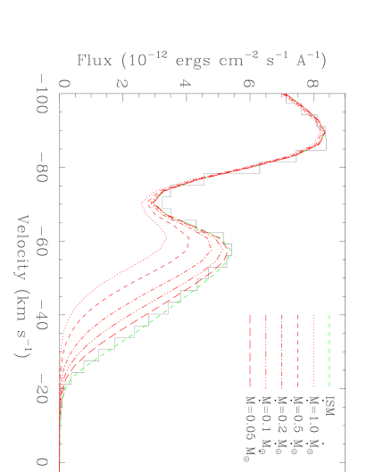
Figure 1: A close-up of the blue side of the H I Lyman-$\alpha$ absorption observed towards $\tau$ Ceti, plotted on a heliocentric velocity scale. The narrow absorption at $-70$ km s^-1 is from interstellar deuterium. The green dashed line shows the ISM absorption, which provides a reasonably good fit to the data. Red lines show additional absorption predicted by astrospheric models assuming different mass-loss rates of $\dot{M}=0.05-1.0~{}\dot{M}_{\odot}$. The $\dot{M}=0.1~{}\dot{M}_{\odot}$ model is assumed to represent an $\dot{M}$ upper limit for $\tau$ Ceti.

The full Lyman-$\alpha$ spectrum and ISM absorption fit to the $\tau$ Ceti data can be found in [12]. Figure 1 zooms into the blue side of the H I Lyman-$\alpha$ absorption profile where the astrospheric absorption would be observed. This is an astrospheric nondetection, meaning that the absorption could be reasonably well fit with ISM absorption alone. Predicted astrospheric absorption is shown for five values of $\dot{M}$, from $\dot{M}=0.05-1.0~{}\dot{M}_{\odot}$. Models actually only exist for $\dot{M}\geq 0.2~{}\dot{M}_{\odot}$, so the $\dot{M}=0.05~{}\dot{M}_{\odot}$ and $\dot{M}=0.1~{}\dot{M}_{\odot}$ models are actually made by extrapolation from the higher $\dot{M}$ models. It is obvious that a $\dot{M}=0.5-1.0~{}\dot{M}_{\odot}$ wind should have yielded easily detectable absorption towards $\tau$ Ceti, but detectability naturally decreases for lower $\dot{M}$ values. It is dubious whether the $\dot{M}=0.05~{}\dot{M}_{\odot}$ model predicts a sufficient amount of absorption to be considered detectable. Relying mostly on subjective judgment, I conclude that it does not and settle on a more conservative $\dot{M}<0.1~{}\dot{M}_{\odot}$ upper limit for $\tau$ Ceti, which is what is reported in Table 1. This is the weakest wind ever measured using the astrospheric absorption technique, slightly lower than the $\dot{M}=0.15~{}\dot{M}_{\odot}$ value for the marginal DK UMa detection [3].

There is one final new $\dot{M}$ measurement listed in Table 1 that has not yet been mentioned, for the transiting exoplanet host star GJ 436 (M3 V). For this star, Lyman-$\alpha$ absorption has been observed during exoplanet transits, implying an evaporating planetary atmosphere, and the amount of absorption has been used to infer the strength of the stellar wind [20]. Thus, this $\dot{M}=0.059^{+0.074}_{-0.040}~{}\dot{M}_{\odot}$ constraint is listed in Table 1 as well, though the measurement is from exoplanetary instead of astrospheric Lyman-$\alpha$ absorption.

3 Revised Wind-Activity Relation

It is natural to look for correlations between wind properties and the properties of the stellar coronae that produce the winds. The most readily available coronal property for comparison is the coronal X-ray luminosity, so values of $\log L_{X}$ are provided in Table 1. Many of these are from ROSAT PSPC measurements [21], but newer Chandra measurements are used when available [22].

Figure 2: A plot of mass loss rate (per unit surface area) versus X-ray surface flux for all main sequence stars with measured winds, analogous to previously published figures [3, 4]. Different symbols are used to represent GK dwarfs, M dwarfs, and subgiant/giant stars. A power law, $\dot{M}\propto F_{X}^{1.29\pm 0.16}$, is fitted to the GK dwarfs where a wind/X-ray relation seems to exist, but this relation seems to fail for stars to the right of the “Wind Dividing Line.” Separate points are plotted for the two members of four binary systems, where for the three less active cases the power law relation is used to estimate the wind contributions of individual stars. In order to yield consistency with stars of similar $F_{X}$, for the $\xi$ Boo binary $\xi$ Boo B is assumed to account for 90% of the wind and $\xi$ Boo A only 10%.

Figure 2 plots mass loss rate per unit surface area versus X-ray surface flux for the stars in Table 1. A correlation is seen for GK dwarfs with $\log F_{X}<6.0$, and a power law relation is fitted to the data. This relation does not extend beyond the $\log F_{X}=6.0$ “Wind Dividing Line,” above which surprisingly weak winds are observed. This figure is very much analogous to similar figures that have been published in the past, including the power law fit and wind dividing line [3, 4]. However, the figure is updated in a number of ways. The most obvious is the inclusion of the four new measurements listed in Table 1. There have also been relatively minor revisions to the X-ray luminosities and stellar radii. The resulting change to the power law relation is insignificant: $\dot{M}\propto F_{x}^{1.29\pm 0.16}$ compared to the previous $\dot{M}\propto F_{x}^{1.34\pm 0.18}$ [3]. The new GJ 892 measurements is completely consistent with the relation. However, the new upper limit for $\tau$ Ceti looks anomalously low. The significance of this inconsistency is marginal, as the $\epsilon$ Ind data point is a similar distance below the power law relation.

Another difference from previous studies lies in our treatment of binary systems. There are four systems listed in Table 1 where both members of the binary lie within the same astrosphere ($\alpha$ Cen AB, 70 Oph AB, 36 Oph AB, and $\xi$ Boo AB), meaning both stellar winds will be contributing to the measured mass-loss rate. For the three binaries that lie entirely to the left of the wind dividing line, the power law relation can be used to estimate the contributions of each individual star to the binary’s collective mass-loss rate, and the results are indicated in both Table 1 and Figure 2. Separate X-ray luminosities are listed for the two stars as well. The most interesting of these three cases is $\alpha$ Cen AB, where the system’s wind is predicted to be dominated by the secondary star, $\alpha$ Cen B, with $\dot{M}=1.54~{}\dot{M}_{\odot}$ compared to $\dot{M}=0.46~{}\dot{M}_{\odot}$ for $\alpha$ Cen A. The $\xi$ Boo AB system is more complicated, with the primary to the left of the dividing line and the secondary to the right. In order for the two stars to be consistent with other stars of similar $F_{X}$, $\xi$ Boo’s wind must be dominated by the secondary. Consistent with past work, a division with $\dot{M}=4.5~{}\dot{M}_{\odot}$ for $\xi$ Boo B and $\dot{M}=0.5~{}\dot{M}_{\odot}$ for $\xi$ Boo A is assumed [23].

The new $\delta$ Pav measurement has interesting implications for the winds of coronal subgiants/giants. Both $\delta$ Pav and $\delta$ Eri imply that inactive subgiants have significantly stronger winds per unit surface area compared to main sequence stars of similar $F_{X}$. This is not a surprising result given that subgiants have lower surface gravities and surface escape speeds than main sequence stars, which should make it easier for coronal material to escape [17]. In contrast, the very active subgiant/giant stars DK UMa and $\lambda$ And seem to have remarkably weak winds, perhaps implying that these stars have strong, global fields that inhibit mass loss in some way.

The GJ 436 measurement in Figure 2 provides a first indication that the winds of inactive M dwarfs may be weaker per unit surface area than GK dwarfs with similar $F_{X}$. Obviously, additional measurements are required to support this conclusion. Fortunately, these measurements should be forthcoming, as a proposed HST Lyman-$\alpha$ survey of 10 M dwarfs within 7 pc has recently been accepted, and these observations should be carried out in the coming year. In the near future, these data will hopefully allow the M dwarf $\dot{M}-F_{X}$ relation to be characterized as well as the GK dwarf relation in Figure 2.

Support for this project was provided by NASA award NNH16AC40I to the Naval Research Laboratory.

References

References

- [1] Neugebauer M, and Snyder C W 1962 Science 138 1095
- [2] Linsky J L, and Wood B E 1996 ApJ 463 254
- [3] Wood B E, Müller H -R, Zank G P, Linsky J L, and Redfield S 2005 ApJ 628 L143
- [4] Wood B E, Müller H -R, Redfield S, and Edelman E 2014 ApJ 781 L33
- [5] van Marle A J, Decin L, and Meliani Z 2014 A&A 561 A152
- [6] Kobulnicky H A et al 2016 ApJS 227 18
- [7] Wood B E, Müller H -R, and Harper G M 2016 ApJ 829 74
- [8] Johnstone C P, Zhilkin A, Pilat-Lohinger E, Bisikalo D, Güdel M, and Lüftinger T 2015 A&A 577 A28
- [9] Lammer H et al 2010 Astrobiology 10 45
- [10] Alvarado-Gómez J D et al 2016 A&A 594 A95
- [11] Shaikhislamov I F et al 2016 ApJ 832 173
- [12] Wood B E, Redfield S, Linsky J L, Müller H -R, and Zank G P 2005 ApJS 159 118
- [13] Sfeir D M, Lallement R, Crifo F, and Welsh B Y 1999 A&A 346 785
- [14] Lallement R, Welsh B Y, Vergely J L, Crifo F, and Sfeir D M 2003 A&A 411 447
- [15] Redfield S, and Linsky J L 2008 ApJ 673 283
- [16] Wood B E, Müller, H -R, and Witte M 2015 ApJ 801 62
- [17] Zachary J, Redfield S, Linsky J L, and Wood B E 2018 ApJ 859 42
- [18] Folsom C P et al 2018 MNRAS in press
- [19] Wood B E, Linsky J L, Müller H -R, and Zank G P 2003 ApJ 591 1210
- [20] Vidotto A A, and Bourrier V 2017 MNRAS 470 4026
- [21] Schmitt J H M H, and Liefke C 2004 A&A 417 651
- [22] Wood B E, Laming J M, Warren H P, and Poppenhaeger K 2018 ApJ in press
- [23] Wood B E, and Linsky J L 2010 ApJ 717 1279