We use higher dimensional bosonization and fermion decoration to construct exactly soluble interacting fermion models to realize fermionic symmetry protected trivial (SPT) orders (which are also known as symmetry protected topological orders) in any dimensions and for generic fermion symmetries $G_{f}$, which can be a non-trivial $Z_{2}^{f}$ extension (where $Z_{2}^{f}$ is the fermion-number-parity symmetry). This generalizes the previous results from group superconhomology of Gu and Wen (arXiv:1201.2648), where $G_{f}$ is assumed to be a trivial $Z_{2}^{f}$ extension. We find that the SPT phases from fermion decoration construction can be described in a compact way using higher groups.

Fermion decoration construction of symmetry protected trivial orders
for fermion systems with any symmetries $G_{f}$ and in any dimensions

I Introduction

We used to think that different phases of matter all come from spontaneous symmetry breaking Landau (1937a, b). In last 30 years, we started to realize that even without symmetry and without symmetry breaking, we can still have different phases of matter, due to a new type of order – topological order Wen (1990); Wen and Niu (1990) (i.e. patterns of long range entanglement Kitaev and Preskill (2006); Levin and Wen (2006); Chen et al. (2010)).

If there is no symmetry breaking nor topological order, it appears that systems must be in the same trivial phase. So it was a surprise to find that even without symmetry breaking and without topological order, systems can still have distinct phases, which are called Symmetry-Protected Trivial (SPT), or synonymously, Symmetry-Protected Topological (SPT) phases Gu and Wen (2009); Chen et al. (2011a). The realization of the existence of SPT orders and the fact that there is no topological order in 1+1D Fannes et al. (1992); Verstraete et al. (2005) lead to a classification of all 1+1D gapped phases of bosonic and fermionic systems with any symmetries Chen et al. (2011b); Schuch et al. (2011); Fidkowski and Kitaev (2011); Chen et al. (2011c), in terms of projective representations Pollmann et al. (2010). It is the first time, after Landau symmetry breaking, that a large class of interacting phases are completely classified.

$G_{f}$	$1+1$D	$2+1$D	$3+1$D	Realization
$Z_{2}\times Z_{2}^{f}$	$\mathbb{Z}_{2}$ [$\mathbb{Z}_{2}$] ($\mathbb{Z}_{2}$)	$\mathbb{Z}_{4}$ [$\mathbb{Z}_{8}$] ($\mathbb{Z}$)	1  [ 1 ] ( 1 )	Double-layer superconductors with layer symmetry
$Z_{4}^{f}$	1  [ ? ] (1)	1  [ ? ] (1)	1  [ ? ] ( 1 )	Charge-$2e$ superconductors with a $180^{\circ}$ spin rotation symmetry or charge-$4e$ superconductors
$Z_{2}^{T}\times Z_{2}^{f}$	$\mathbb{Z}_{4}$ [$\mathbb{Z}_{4}$] ($\mathbb{Z}$)	1  [ 1 ] ( 1 )	1  [ 1 ] ( 1 )	Charge-$2e$ superconductors with coplanar spin order
$Z_{4}^{T,f}$	$\mathbb{Z}_{2}$ [$\mathbb{Z}_{2}$] ($\mathbb{Z}_{2}$)	1  [$\mathbb{Z}_{2}$] ($\mathbb{Z}_{2}$)	$\mathbb{Z}_{4}$ [$\mathbb{Z}_{16}$] ($\mathbb{Z}$)	Charge-$2e$ superconductors with spin-orbital coupling
$(U_{1}^{f}\rtimes_{\phi}Z_{4}^{T,f})/Z_{2}$	1  [ 1 ] (1)	1  [$\mathbb{Z}_{2}$] ($\mathbb{Z}_{2}$)	$\mathbb{Z}_{2}^{3}$ [$\mathbb{Z}_{2}^{3}$] ($\mathbb{Z}_{2}$)	Insulator with spin-orbital coupling
$SU_{2}^{f}$	1  [ 1 ] (1)	$\mathbb{Z}$  [ $\mathbb{Z}$ ] ($\mathbb{Z}$)	1  [ 1 ] ( 1 )	Charge-$2e$ spin-singlet superconductor
$Z_{2}\times Z_{4}\times Z_{2}^{f}$	$\mathbb{Z}_{2}^{3}$ [?] ($\mathbb{Z}_{2}^{7}$)	$8\cdot 16$ [?] ($\mathbb{Z}^{7}$)	$2\cdot 4$ [$\mathbb{Z}_{2}\times\mathbb{Z}_{4}$] (1)

Table 1: A table for $G_{f}$-symmetric fermionic SPT orders obtained via the fermion decoration.Gu and Wen (2014) We either list the group that describes the SPT phases or the number of SPT phases (both including the trivial one). Those fermionic SPT phases have no topological order, i.e. they become trivial if we break the symmetry down to $Z_{2}^{f}$. The numbers in [ ] are results from spin-cobordism approach Kapustin et al. (2015); Freed and Hopkins (2016); Wang et al. (2018). The numbers in ( ) are for non-interacting fermionic SPT phases, Kitaev (2009); Schnyder et al. (2008); Wen (2012). Note that the numbers given in LABEL:K0986,SRF0825,W11116341,KTT1429 are for SIT orders which include both fermionic SPT orders and invertible fermionic topological orders, while the above numbers only include fermionic SPT orders. The number, for example, $8\cdot 16$ means that the $256$ SPT phases can be divided into 8 classes with 16 SPT phases in each class. The SPT phases in the same class only differ by stacking bosonic SPT phases from fermion pairs. The last column indicates how to realize those fermionic SPT phases by electronic systems.

In higher dimensions, the SPT orders, or more generally symmetric invertible topological (SIT) orders, in bosonic systems can be systematically described by group cohomology theory Chen et al. (2013); Vishwanath and Senthil (2013); Wen (2015), cobordism theory Kapustin (2014b); Freed and Hopkins (2016), or generalized cohomology theory Freed and Hopkins (2016); Gaiotto and Johnson-Freyd (2017). The SPT and SIT orders in fermionic systems can be systematically described by group super-cohomology theory Gu and Wen (2014); Cheng et al. (2018); Gaiotto and Kapustin (2016); Kapustin and Thorngren (2017); Wang and Gu (2017), or spin cobordism theory Kapustin et al. (2015); Freed and Hopkins (2016); Wang et al. (2018). In 2+1D, the SPT orders in bosonic or fermionic systems can also be systematically classified by the modular extensions of $\mathcal{R}\mathrm{ep}(G_{b})$ or $\mathrm{s}\mathcal{R}\mathrm{ep}(G_{f})$ Lan et al. (2016). Here $\mathcal{R}\mathrm{ep}(G_{b})$ is the symmetric fusion category formed by representations of the boson symmetry $G_{b}$ where all representations are bosonic, and $\mathrm{s}\mathcal{R}\mathrm{ep}(G_{f})$ is the symmetric fusion category formed by representations of the fermion symmetry $G_{f}=Z_{2}^{f}\leftthreetimes G_{b}$ where the representations with non-zero $Z_{2}^{f}$ charge are fermionic. ($Z_{2}^{f}\leftthreetimes G_{b}$ denote an extension of $G_{b}$ by the fermion-number-parity symmetry $Z_{2}^{f}$.)

For SPT orders in fermionic systems, the modular extension approach in 2+1D can handle generic fermion symmetry $G_{f}=Z_{2}^{f}\leftthreetimes G_{b}$. However, in higher dimensions, the group super-cohomology theory can only handle a special form of fermion symmetry $G_{f}=Z_{2}^{f}\times G_{b}$. In this paper, we will develop a more general group super-cohomology theory for SPT orders of fermion systems based on the decoration constructionChen et al. (2014) by fermions,Gu and Wen (2014) which covers generic fermion symmetry $G_{f}$ beyond $Z_{2}^{f}\times G_{b}$. The symmetry group $G_{f}$ can also include time reversal symmetry, and in this case, the fermions can be time-reversal singlet or Kramers doublet. Our approach works in any dimensions. But our theory does not covers the fermionic SPT orders obtained by decorating symmetry line-defectsCheng et al. (2018); Kapustin and Thorngren (2017); Wang and Gu (2017) with Majorana chains (i.e. the $p$-wave topological superconducting chains Kitaev (2001)).

Our theory is constructive in nature. We have constructed exactly soluble local fermionic path integrals (in the bosonized form) to realize the fermionic SPT orders systematically. The simple physical results of this paper is summarized in Table 1. A mathematical summary of the results is represented Section III (and in Section VIII where more details are given). However, one needs to use mathematical language of cohomology or higher group to state the results precisely.

We note that there are seven non-trivial fermionic $(U_{1}^{f}\rtimes_{\phi}Z_{4}^{T,f})/Z_{2}$-SPT phases in 3+1D, while non-interacting fermions only realize one of them. Other SPT phases are obtained by stacking the bosonic $(U_{1}\rtimes_{\phi}Z_{2}^{T})$-SPT phases formed by electron-hole pairs.

II Notations and conventions

Let us first explain some notations used in this paper. We will use extensively the mathematical formalism of cochains, coboundaries, and cocycles, as well as their higher cup product $\underset{{\scriptscriptstyle k}}{\smile}$, Steenrod square $\text{Sq}^{k}$, and the Bockstrin homomorphism $\beta_{n}$. A brief introduction can be found in Appendix A. We will abbreviate the cup product $a\smile b$ as $ab$ by dropping $\smile$. We will use a symbol with bar, such as $\bar{a}$ to denote a cochain on the classifying space ${\cal B}$ of a group or higher group. We will use $a$ to denote the corresponding pullback cochain on space-time ${\cal M}^{d+1}$: $a=\phi^{*}\bar{a}$, where $\phi$ is a homomorphism of complexes $\phi:{\cal M}^{d+1}\to{\cal B}$. In this paper, when we refer ${\mathbb{R}/\mathbb{Z}}$-valued cocycle or coboundary we really mean ${\mathbb{R}/\mathbb{Z}}$-valued almost-cocycle and almost-coboundary (see Appendix B.

We will use $\overset{\scriptscriptstyle n}{=}$ to mean equal up to a multiple of $n$, and use $\overset{\scriptscriptstyle\hskip 1.0pt\mathrm{d}}{=}$ to mean equal up to $\hskip 1.0pt\mathrm{d}f$ (i.e. up to a coboundary). We will use $\lfloor x\rfloor$ to denote the largest integer smaller than or equal to $x$, and $\langle l,m\rangle$ to denote the greatest common divisor of $l$ and $m$ ($\langle 0,m\rangle\equiv m$).

Also, we will use $Z_{n}=\{1,\hskip 1.0pt\mathrm{e}^{\hskip 1.0pt\mathrm{i}\hskip 1.0pt\frac{2\pi}{n}},\hskip 1.0pt\mathrm{e}^{\hskip 1.0pt\mathrm{i}\hskip 1.0pt2\frac{2\pi}{n}},\cdots,\hskip 1.0pt\mathrm{e}^{\hskip 1.0pt\mathrm{i}\hskip 1.0pt(n-1)\frac{2\pi}{n}}\}$ to denote an Abelian group, where the group multiplication is “$*$”. We use $\mathbb{Z}_{n}=\{\lfloor-\frac{n}{2}+1\rfloor,\lfloor-\frac{n}{2}+1\rfloor+1,\cdots,\lfloor\frac{n}{2}\rfloor\}$ to denote an integer lifting of $Z_{n}$, where “+” is done without mod-$n$. In this sense, $\mathbb{Z}_{n}$ is not a group under “+”. But under a modified equality $\overset{\scriptscriptstyle n}{=}$, $\mathbb{Z}_{n}$ is the $Z_{n}$ group under “+”. Similarly, we will use ${\mathbb{R}/\mathbb{Z}}=(-\frac{1}{2},\frac{1}{2}]$ to denote an $\mathbb{R}$-lifting of $U_{1}$ group. Under a modified equality $\overset{\scriptscriptstyle 1}{=}$, ${\mathbb{R}/\mathbb{Z}}$ is the $U_{1}$ group under “+”. In this paper, there are many expressions containing the addition “+” of $\mathbb{Z}_{n}$-valued or ${\mathbb{R}/\mathbb{Z}}$-valued, such as $a^{\mathbb{Z}_{n}}_{1}+a^{\mathbb{Z}_{n}}_{2}$ where $a^{\mathbb{Z}_{n}}_{1}$ and $a^{\mathbb{Z}_{n}}_{2}$ are $\mathbb{Z}_{n}$-valued. Those additions “+” are done without mod $n$ or mod 1. In this paper, we also have expressions like $\frac{1}{n}a^{\mathbb{Z}_{n}}_{1}$. Such an expression convert a $\mathbb{Z}_{n}$-valued $a^{\mathbb{Z}_{n}}_{1}$ to a ${\mathbb{R}/\mathbb{Z}}$-valued $\frac{1}{n}a^{\mathbb{Z}_{n}}_{1}$, by viewing the $\mathbb{Z}_{n}$-value as a $\mathbb{Z}$-value. (In fact, $\mathbb{Z}_{n}$ is a $\mathbb{Z}$ lifting of $Z_{n}$.)

We introduced a symbol $\leftthreetimes$ to construct fiber bundle $X$ from the fiber $F$ and the base space $B$:

$$pt\to F\to X=F\leftthreetimes B\to B\to pt.$$ (1)

We will also use $\leftthreetimes$ to construct group extension of $H$ by $N$ Morandi (1997):

$$1\to N\to N\leftthreetimes_{e_{2},\alpha}H\to H\to 1.$$ (2)

Here $e_{2}\in H^{2}[H;Z(N)]$ and $Z(N)$ is the center of $N$. Also $H$ may have a non-trivial action on $Z(N)$ via $\alpha:H\to\text{Aut}(N)$. $e_{2}$ and $\alpha$ characterize different group extensions.

We will also use the notion of higher group in some part of the paper. Here we will treat a $d$-group ${\cal B}(\Pi_{1},1;\Pi_{2},2;\cdots)$ as a special one-vertex triangulation of a manifold $K$ that satisfy $\pi_{n}(K)=\Pi_{n}$ (with unlisted $\Pi_{n}$ treated as 0, see LABEL:ZLW and Appendix L). We see that $\Pi_{1}$ is a group and $\Pi_{n}$, $n\geq 2$, are Abelian groups. The 1-group ${\cal B}(G,1)$ is nothing but an one-vertex triangulation of the classifying space of $G$. We will abbreviate ${\cal B}(G,1)$ as ${\cal B}G$. (More precisely, the so called one-vertex triangulation is actually a simplicial set.)

III A brief mathematical summary

In this paper, we use a higher dimensional bosonizationWen (2017); Kapustin and Thorngren (2017) to describe local fermion systems in $d+1$-dimensional space-time via a path integral on a random space-time lattice (which is called a space-time complex that triangulate the space-time manifold). This allows us to construct exactly soluble path integrals on space-time complexes based on fermion decoration constructionGu and Wen (2014) to systematically realize a large class of fermionic SPT orders with a generic fermion symmetry $G_{f}=Z_{2}^{f}\leftthreetimes G_{b}$. This generalizes the previous result of LABEL:GW1441,CG150101313 that only deal with fermion symmetry of form $G_{f}=Z_{2}^{f}\times G_{b}$. The constructed models are exactly soluble since the partition functions are invariant under any re-triangulation of the space-time.

The constructed exactly soluble path integrals and the corresponding fermionic SPT phases are labeled by some data. Those data can be described in a compact form using terminology of higher group ${\cal B}(\Pi_{1},1;\Pi_{2},2;\cdots)$ (see Appendix L for details). We note that, for a $d$-group ${\cal B}(G,1;Z_{2},d)$ (i.e. a complex with only one vertex), its links are labeled by group elements $g\in G$. This gives rise to the so called canonical $G$-valued 1-cochain $\bar{a}$ on the complex ${\cal B}(G,1;Z_{2},d)$. On each $d$-simplex in ${\cal B}(G,1;Z_{2},d)$ we also have a $Z_{2}$ label. This gives us the canonical $\mathbb{Z}_{2}$-valued $d$-cochain $\bar{f}_{d}$ on the complex ${\cal B}(G,1;Z_{2},d)$. Now, we can are ready to state our results:

1. Characterization data without time reversal: For unitary symmetry $G_{f}$, the fermionic SPT phases obtained via fermion decoration are described by a pair $(\varphi,\nu_{d+1})$, where $\varphi:{\cal B}(G_{f}\leftthreetimes SO_{\infty},1)\to{\cal B}_{f}(SO_{\infty},1;Z_{2},d)$ is a homomorphism between two higher groups and $\nu_{d+1}$ is a $\mathbb{R}/\mathbb{Z}$-valued $d+1$-cochain on ${\cal B}(G_{f}\leftthreetimes SO_{\infty},1)$ that trivializes the pullback of a $\mathbb{R}/\mathbb{Z}$-valued $d+2$-cocycle $\bar{\omega}_{d+2}=\frac{1}{2}\text{Sq}^{2}\bar{f}_{d}+\frac{1}{2}\bar{f}_{d}\bar{\text{w}}_{2}$ on ${\cal B}_{f}(SO_{\infty},1;Z_{2},d)$, i.e. $-\text{d}\nu_{d+1}=\text{d}\varphi^{*}\bar{\omega}_{d+2}$.
   Here $\bar{f}_{d}$ is the canonical $d$-cochain on ${\cal B}_{f}(SO_{\infty},1;Z_{2},d)$, and $\bar{\rm w}_{n}$ is the $n^{\text{th}}$ Stiefel-Whitney class constructed from canonical $d$-cochain $\bar{a}$ on ${\cal B}_{f}(SO_{\infty},1;Z_{2},d)$. Note that $\bar{a}$ can be viewed as the $SO_{\infty}$ connection of a $SO_{\infty}$ bundle over ${\cal B}_{f}(SO_{\infty},1;Z_{2},d)$.

2. Characterization data with time reversal: In the presence of time reversal symmetry $G_{f}=G_{f}^{0}\leftthreetimes Z_{2}^{T}$, we find that the fermionic SPT phases obtained via fermion decoration are described by a pair $(\varphi,\nu_{d+1})$, where $\varphi:{\cal B}(G_{f}^{0}\leftthreetimes O_{\infty},1)\to{\cal B}_{f}(O_{\infty},1;Z_{2},d)$ is a homomorphism between two higher groups and $\nu_{d+1}$ is a $\mathbb{R}/\mathbb{Z}$-valued $d+1$-cochain on ${\cal B}(G_{f}^{0}\leftthreetimes O_{\infty},1)$ that trivializes the pullback of a $\mathbb{R}/\mathbb{Z}$-valued $d+2$-cocycle $\bar{\omega}_{d+2}=\frac{1}{2}\text{Sq}^{2}\bar{f}_{d}+\frac{1}{2}\bar{f}_{d}(\bar{\text{w}}_{2}+\bar{\text{w}}_{1}^{2})$ on ${\cal B}_{f}(O_{\infty},1;Z_{2},d)$, i.e. $-\text{d}\nu_{d+1}=\text{d}\varphi^{*}\bar{\omega}_{d+2}$.

3. Model construction and SPT invariant: Using the data $(\varphi,\nu_{d+1})$, we can write down the explicit re-triangulation invariant path integral that describes a local fermion model (in bosonized form) that realized the corresponding SPT phases (see eqn. (VIII.1), eqn. (60), and eqn. (56)). We can also write down the SPT invariantWen (2014); Hung and Wen (2014); Kapustin (2014b); Wen (2015); Kapustin et al. (2015) that characterize the resulting fermionic SPT phase (see eqn. (VIII.2), eqn. (VIII.2), and eqn. (VIII.5)). Those bosonized fermion path integrals, eqn. (VIII.1), eqn. (60), and eqn. (56), and the corresponding SPT invariants, eqn. (VIII.2), eqn. (VIII.2), and eqn. (VIII.5), are the main results of this paper.

4. Equivalence relation: Only the pairs $(\varphi,\nu_{d+1})$ that give rise to distinct SPT invariants correspond to distinct SPT phases. The pairs $(\varphi,\nu_{d+1})$ that give rise to the same SPT invariant are regarded as equivalent. In particular, two homotopically connected $\varphi$’s are equivalent and two $\nu_{d+1}$’s differ by a coboundary are equivalent.

The data $(\varphi,\nu_{d+1})$ cover all the fermion SPT states obtained via fermion decoration. But they do not include the fermion SPT states obtained via decoration of chains of 1+1D topological $p$-wave superconducting states, but may include some fermion SPT states obtained via decoration of sheets of 2+1D topological $p$-wave superconducting state.

IV Exactly soluble models for bosonic SPT phases

Let us first review the construction of exactly soluble models for bosonic SPT orders with on-site symmetry group $G_{b}$ Chen et al. (2013). The same line of thinking will also be used in our discussions of fermionic SPT phases.

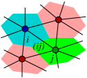
Figure 1: (Color online) The vertices $i$ and $j$ mark the regions with order parameter $g_{i}$ and $g_{j}$. The link labeled by $(ij)$ connects the vertices $i$ and $j$.

IV.1 Constructing path integral

We start with a phase that breaks the $G_{b}$ symmetry completely. Then we consider the quantum fluctuations of the $G_{b}$-symmetry-breaking domains which restore the symmetry. We mark each domain with a vertex (see Fig. 1), which form a space-time complex ${\cal M}^{d+1}$ (see Appendix A for details). So the quantum fluctuations of the domains are described by the degrees of freedom given by $g_{i}\in G_{b}$ on each vertex $i$. In other words, the degrees of freedom is a $G_{b}$-valued 0-cochain field $g\in C^{0}({\cal M}^{d+1};G_{b})$.

In order to probe the SPT orders in a universal way, we can add the symmetry twist to the system (i.e. gauging the symmetry) Levin and Gu (2012); Hung and Wen (2014); Wen (2014); Kapustin (2014b). This is done by adding a fixed $G_{b}$-valued 1-cochain field $A\in C^{1}({\cal M}^{d+1};G_{b})$ with $A^{G_{b}}_{ij}\in G_{b}$ on each link $(ij)$ that connect two vertices $i$ and $j$. The cochain field $A$ satisfy the flat condition

$$(\delta A^{G_{b}})_{ijk}\equiv A^{G_{b}}_{ij}A^{G_{b}}_{jk}A^{G_{b}}_{ki}=1,$$ (3)

where we have assumed $A^{G_{b}}_{ij}=(A^{G_{b}}_{ji})^{-1}$. Those flat 1-cochain field will be called 1-cocycle field. The collection of those $G_{b}$-valued 1-cocycle fields will be denoted by $Z^{1}({\cal M}^{d+1},G_{b})$. We stress that the 1-cocycle field $A$ is a fixed background field that do not fluctuate.

From the dynamical $g$ and non-dynamical background field $A^{G_{b}}$, we can construct an effective dynamic $G_{b}$-valued 1-cocycle field $a^{G_{b}}$ whose values on links are given by

$$a^{G_{b}}_{ij}=g_{i}A^{G_{b}}_{ij}g_{j}^{-1}.$$ (4)

Using such an effective dynamic field, we can construct our model as

$$Z({\cal M}^{d+1},A^{G_{b}})=\sum_{g\in C^{0}({\cal M}^{d+1};{G_{b}})}\hskip-10.00002pt\hskip 1.0pt\mathrm{e}^{\hskip 1.0pt\mathrm{i}\hskip 1.0pt2\pi\int_{{\cal M}^{d+1}}\omega_{d+1}(a^{G_{b}})},$$ (5)

where $\omega_{d+1}(a^{G_{b}})$ is $\mathbb{R}/\mathbb{Z}$-valued $d$-cochain: $\omega_{d+1}(a^{G_{b}})\in C^{d+1}({\cal M}^{d+1};\mathbb{R}/\mathbb{Z})$, whose value on a $d+2$-simplex $(i_{0}i_{1}\cdots i_{d+1})$ is a function of $a^{G_{b}}_{i_{0}i_{1}},a^{G_{b}}_{i_{0}i_{2}},a^{G_{b}}_{i_{1}i_{2}},\cdots$: $(\omega_{d+1})_{i_{0}i_{1}\cdots i_{d+1}}=\omega_{d+1}(a^{G_{b}}_{i_{0}i_{1}},a^{G_{b}}_{i_{0}i_{2}},a^{G_{b}}_{i_{1}i_{2}},\cdots)$. Note that $a^{G_{b}}$ also satisfies the flat condition

$$(\delta a^{G_{b}})_{ijk}\equiv a^{G_{b}}_{ij}a^{G_{b}}_{jk}a^{G_{b}}_{ki}=1.$$ (6)

So we say $a^{G_{b}}\in Z^{1}({\cal M}^{d+1};{G_{b}})$. In this case the function $\omega_{d+1}(a^{G_{b}}_{i_{0}i_{1}},a^{G_{b}}_{i_{0}i_{2}},a^{G_{b}}_{i_{1}i_{2}},\cdots)$ only depends on $a^{G_{b}}_{i_{0}i_{1}},a^{G_{b}}_{i_{1}i_{2}},a^{G_{b}}_{i_{2}i_{3}}$, etc , since other variables are determined from those variables:

$$(\omega_{d+1})_{i_{0}i_{1}\cdots i_{d+1}} =\omega_{d+1}(a^{G_{b}}_{i_{0}i_{1}},a^{G_{b}}_{i_{1}i_{2}},a^{G_{b}}_{i_{2}i_{3}},\cdots).$$ (7)

We note that the assignment of $a^{G_{b}}_{ij}\in{G_{b}}$ on each link $(ij)$ can be viewed as a map $\phi$ (a homomorphism of complexes) from space-time complex ${\cal M}^{d+1}$ to ${\cal B}G_{b}$ which is a simplicial complex that model the classifying space $B{G_{b}}$ of the group ${G_{b}}$. The $d+1$-cochain $\omega_{d+1}(a^{G_{b}})$ can be viewed as a pull back of a cochain $\bar{\omega}_{d+1}(\bar{a}^{G_{b}})$ in the classifying space ${\cal B}{G_{b}}$: $\bar{\omega}_{d+1}(\bar{a}^{G_{b}})\in C^{d+1}({\cal B}{G_{b}};\mathbb{R}/\mathbb{Z})$. Here $\bar{\omega}_{d+1}(\bar{a}^{G_{b}})$ is a function of the canonical 1-cochain $\bar{a}^{G_{b}}$. Note that links in ${\cal B}{G_{b}}$ are labeled by elements of $G_{b}$, which give rise to the canonical 1-cochain $\bar{a}^{G_{b}}$ on ${\cal B}{G_{b}}$ (see LABEL:ZLW and Appendix L). The above can be written as

$$a^{G_{b}} =\phi^{*}\bar{a}^{G_{b}},\ \ \ \$$

$$\omega_{d+1}(a^{G_{b}}) =\phi^{*}\bar{\omega}_{d+1}(\bar{a}^{G_{b}}).$$ (8)

IV.2 Making path integral exactly soluble

To make the model exactly soluble, we require $\omega_{d+1}$ to be a pullback of a cocycle $\bar{\omega}_{d+1}$ in the classifying space $B{G_{b}}$:

$$\hskip 1.0pt\mathrm{d}\bar{\omega}_{d+1}(\bar{a}^{G_{b}})\overset{\scriptscriptstyle 1}{=}0\ \ \text{ or }\ \ \bar{\omega}_{d+1}(\bar{a}^{G_{b}})\in Z^{d+1}({\cal B}{G_{b}};\mathbb{R}/\mathbb{Z}).$$ (9)

Why the above condition make our model exactly soluble? Let us compare two action amplitudes $\hskip 1.0pt\mathrm{e}^{\hskip 1.0pt\mathrm{i}\hskip 1.0pt2\pi\int_{{\cal M}^{d+1}}\omega_{d+1}(a^{G_{b}})}$ and $\hskip 1.0pt\mathrm{e}^{\hskip 1.0pt\mathrm{i}\hskip 1.0pt2\pi\int_{{\cal M}^{d+1}}\omega_{d+1}(a^{G_{b}\prime})}$ for two different field values $a^{G_{b}}$ and $a^{G_{b}\prime}$. We like to show that if $a^{G_{b}}$ and $a^{G_{b}\prime}$ can homotopically deform into each other, then $\hskip 1.0pt\mathrm{e}^{\hskip 1.0pt\mathrm{i}\hskip 1.0pt2\pi\int_{{\cal M}^{d+1}}\omega_{d+1}(a^{G_{b}})}=\hskip 1.0pt\mathrm{e}^{\hskip 1.0pt\mathrm{i}\hskip 1.0pt2\pi\int_{{\cal M}^{d+1}}\omega_{d+1}(a^{G_{b}\prime})}$. But $a^{G_{b}}$ and $a^{G_{b}\prime}$ are discrete fields on discrete lattice. It seems that they can never homotopically deform into each other, in the usual sense.

To define the homotopical deformation for discrete fields on discrete lattice, we try to find a flat connection $\tilde{a}^{G_{b}}$ on a complex ${\cal M}^{d+1}\times I$ in one higher dimension, such that $\tilde{a}^{G_{b}}=a^{G_{b}}$ on one boundary of ${\cal M}^{d+1}\times I$, and $\tilde{a}^{G_{b}}=a^{G_{b}\prime}$ on the other boundary of ${\cal M}^{d+1}\times I$. If such a field $\tilde{a}^{G_{b}}$ exists, then we say $a^{G_{b}}$ and $a^{G_{b}\prime}$ can homotopically deform into each other. In this case, we find that

$$\frac{\hskip 1.0pt\mathrm{e}^{\hskip 1.0pt\mathrm{i}\hskip 1.0pt2\pi\int_{{\cal M}^{d+1}}\omega_{d+1}(a^{G_{b}\prime})}}{\hskip 1.0pt\mathrm{e}^{\hskip 1.0pt\mathrm{i}\hskip 1.0pt2\pi\int_{{\cal M}^{d+1}}\omega_{d+1}(a^{G_{b}})}} =\hskip 1.0pt\mathrm{e}^{\hskip 1.0pt\mathrm{i}\hskip 1.0pt2\pi\int_{{\cal M}^{d+1}\times I}\hskip 1.0pt\mathrm{d}\omega_{d+1}(\tilde{a}^{G_{b}})}$$

$$=\hskip 1.0pt\mathrm{e}^{\hskip 1.0pt\mathrm{i}\hskip 1.0pt2\pi\int_{\phi({\cal M}^{d+1}\times I)}\hskip 1.0pt\mathrm{d}\bar{\omega}_{d+1}(\bar{a}^{G_{b}})},$$ (10)

where $\phi$ is a homomorphism from ${\cal M}^{d+1}\times I$ to ${\cal B}G_{b}$. Therefore $\hskip 1.0pt\mathrm{e}^{\hskip 1.0pt\mathrm{i}\hskip 1.0pt2\pi\int_{{\cal M}^{d+1}}\omega_{d+1}(a^{G_{b}})}=\hskip 1.0pt\mathrm{e}^{\hskip 1.0pt\mathrm{i}\hskip 1.0pt2\pi\int_{{\cal M}^{d+1}}\omega_{d+1}(a^{G_{b}\prime})}$ if $\hskip 1.0pt\mathrm{d}\bar{\omega}_{d+1}(\bar{a}^{G_{b}})\overset{\scriptscriptstyle 1}{=}0$ and if $a^{G_{b}}$ can homotopically deform into $a^{G_{b}\prime}$ without breaking the flat condition eqn. (6).

Let us view $a^{G_{b}}$ and $a^{G_{b}\prime}$ to be equivalent, if they can homotopically deform into each other. This define the “gauge equivalent” configurations. It turns out that two configurations $a^{G_{b}}$ and $a^{G_{b}\prime}$ are equivalent if and only if they are connected by a gauge transformation

$$a^{G_{b}\prime}_{ij}=h_{i}a^{G_{b}}_{ij}h_{j}^{-1},\ \ \ h_{i}\in G_{b}.$$ (11)

Thus the action amplitude $\hskip 1.0pt\mathrm{e}^{\hskip 1.0pt\mathrm{i}\hskip 1.0pt2\pi\int_{{\cal M}^{d+1}}\omega_{d+1}(a^{G_{b}})}$ only depends on the equivalent classes of the field configurations $a^{G_{b}}$. Since the homotopical deformations represent the most but a finite kinds of the fluctuations of $a^{G_{b}}$, there is only a finite number of equivalent classes. Thus the action amplitude $\hskip 1.0pt\mathrm{e}^{\hskip 1.0pt\mathrm{i}\hskip 1.0pt2\pi\int_{{\cal M}^{d+1}}\omega_{d+1}(a^{G_{b}})}$ only dependents on a finite number of equivalent classes of $a^{G_{b}}$, and the partition function $Z({\cal M}^{d+1})$ can be calculated exactly. In this case, we say the model is exactly soluble. We see that different $\omega_{d+1}(a^{G_{b}})\in{\cal Z}^{d+1}(G_{b};\mathbb{R}/\mathbb{Z})$ characterize different exactly soluble models.

The space ${\cal Z}^{d+1}(G_{b};\mathbb{R}/\mathbb{Z})$ is not connected. Each connected piece describes models in the same phase. Thus the different phases of the models are given by $\pi_{0}[{\cal Z}^{d+1}(G_{b};\mathbb{R}/\mathbb{Z})]=H^{d+1}({\cal B}G_{b},\mathbb{R}/\mathbb{Z})$. Those models do not spontaneously break the ${G_{b}}$-symmetry. Without symmetry twist $A^{G_{b}}_{ij}=1$, the volume-independent partition function $Z^{\text{top}}({\cal M}^{d+1})$ Kong and Wen (2014); Wen and Wang (2018) of the above models is $Z^{\text{top}}({\cal M}^{d+1})=1$ for any closed oriented manifolds. So the models have no topological orders, and realize only SPT orders. We see that the SPT orders described by those models are labeled by $H^{d+1}({\cal B}G_{b},\mathbb{R}/\mathbb{Z})$.

IV.3 Including time reversal symmetry $Z_{2}^{T}$

In the above, we did not include time reversal symmetry described by group $Z_{2}^{T}$. In the presence of time reversal symmetry the full symmetry group $G_{b}$ is an extension of $Z_{2}^{T}$: $G_{b}=G_{b}^{0}\leftthreetimes Z_{2}^{T}$, where $G_{b}^{0}$ is the unitary on-site symmetry. In this case, the dynamical variable is still $g_{i}\in G_{b}$, the symmetry twist is still describe by $A^{G_{b}}_{ij}\in G_{b}$. But the symmetry twist satisfy a constraint: The natural projection $G_{b}\to Z_{2}^{T}$ reduce the $G_{b}$ connection $A^{G_{b}}_{ij}$ to a $Z_{2}^{T}$ connection $A^{T}_{ij}\in Z_{2}^{T}$. $A^{T}_{ij}$ describes a $Z_{2}$ bundle over the space-time ${\cal M}^{d+1}$. The tangent bundle of space-time ${\cal M}^{d+1}$ give rise to a $O_{d+1}$ bundle over ${\cal M}^{d+1}$. From the $O_{d+1}$ bundle we can get its determinant bundle, which is also a $Z_{2}$ bundle over ${\cal M}^{d+1}$. Such a $Z_{2}$ bundle must be the homotopic equivalent to the $Z_{2}$ bundle described by the $Z_{2}^{T}$ connection $A^{T}_{ij}$. In other words,

$$A^{T}\overset{\scriptscriptstyle 2,\hskip 1.0pt\mathrm{d}}{=}{\rm w}_{1},$$ (12)

where ${\rm w}_{n}$ is the $n^{\text{th}}$ Stiefel-Whitney class of ${\cal M}^{d+1}$. In addition to the above constraint, we also require the Lagrangian $2\pi\omega_{d+1}(a^{G_{b}})$ to have a time reversal symmetry. As pointed out in LABEL:CGL1314, this can be achieved by requiring $\omega_{d+1}(a^{G_{b}})$ to be a ${\mathbb{R}/\mathbb{Z}}$-valued cocycle where $Z_{2}^{T}$ has a non-trivial action on the value ${\mathbb{R}/\mathbb{Z}}\to-{\mathbb{R}/\mathbb{Z}}$.

We see that, to include time reversal symmetry, we need to extend a space-time symmetry, space-time refection $Z_{2}^{T}$, by the internal symmetry $G_{b}^{0}$ to obtain the full symmetry group $G_{b}$. As shown in LABEL:CGL1314,K1459, in this case, the SPT states are labeled by the elements in $H^{d+1}({\cal B}G_{b},(\mathbb{R}/\mathbb{Z})_{T})$ where time reversal in $G_{b}$ has a non-trivial action on the value $T:\mathbb{R}/\mathbb{Z}\to-\mathbb{R}/\mathbb{Z}$. Also, the differential operator $\hskip 1.0pt\mathrm{d}$ should be understood as the one with this non-trivial action.

IV.4 Classification of bosonic SPT phases

However, $H^{d+1}({\cal B}G_{b},(\mathbb{R}/\mathbb{Z})_{T})$ fail to cover all bosonic SPT orders Vishwanath and Senthil (2013). It misses the SPT orders obtained by decorating Chen et al. (2014) symmetry defects with the invertible bosonic topological orders Kong and Wen (2014); Kapustin (2014b); Freed and Hopkins (2016). This problem can be fixed if we replace ${G_{b}}$ by $G_{bO}=G_{b}^{0}\leftthreetimes O_{\infty}$, where $O_{n}$ is the $n$-dimensional orthogonal group. This generalizes the extension $G_{b}=G_{b}^{0}\leftthreetimes Z_{2}^{T}$ discussed in the last section to include time reversal symmetry. The time reversal symmetry is included in $O_{\infty}$ as the disconnected component, which is denoted by $Z_{2}^{T}$.

After replacing ${G_{b}}$ by ${G_{bO}}$, we can obtain local bosonic models that realize more general SPT states, as well as the bosonic SIT orders Wen (2015):

$$Z({\cal M}^{d+1})=\sum_{g\in C^{0}({\cal M}^{d+1};G_{bO})}\hskip-10.00002pt\hskip 1.0pt\mathrm{e}^{\hskip 1.0pt\mathrm{i}\hskip 1.0pt2\pi\int_{{\cal M}^{d+1}}\omega_{d+1}(a^{G_{bO}})},$$ (13)

where $(a^{G_{bO}})_{ij}=g_{i}A^{bO}_{ij}g_{j}^{-1}$ and $A^{bO}_{ij}\in G_{bO}$. Also $\omega_{d+1}(a^{G_{bO}})$ is the pullback of $\bar{\omega}_{d+1}(\bar{a}^{G_{bO}})\in{\cal Z}^{d+1}[{\cal B}G_{bO};(\mathbb{R}/\mathbb{Z})_{T}]$.

We like to stress that the $A^{bO}_{ij}$ is not the most general connection of a $G_{bO}$ bundle on ${\cal M}^{d+1}$. We may project $A^{bO}_{ij}\in G_{bO}$ to $A^{O}_{ij}\in O_{\infty}$ via the natural projection $G_{bO}\to O_{\infty}$. The resulting $A^{O}_{ij}$ describes a $O_{\infty}$ bundle on ${\cal M}^{d+1}$, and such a $O_{\infty}$ bundle must be the tangent bundle of ${\cal M}^{d+1}$ (extended by a trivial bundle).

What is the physical meaning of the above statement “the resulting $A^{O}_{ij}$ describes the tangent bundle of ${\cal M}^{d+1}$”? We can cover the space-time manifold ${\cal M}^{d+1}$ with meany simple patches. On each patch, $(a^{G_{bO}})_{ij}=g_{i}A^{bO}_{ij}g_{j}^{-1}$. On the overlaping region of two patches, $g_{i},A^{bO}_{ij}$ and $g_{i}^{\prime},A^{bO\prime}_{ij}$ on the two patches are related

$$g_{i}^{\prime}=g_{i}h_{i},\ A^{bO\prime}_{ij}=h_{i}^{-1}A^{bO}_{ij}h_{j},\ h_{i}\in G_{bO}=G_{b}^{0}\leftthreetimes O_{\infty}.$$ (14)

We require that the projection $h_{i}\to h^{O}_{i}\in O_{\infty}$ corresponds to the $O_{d+1}$ space-time rotation. Thus the field $g_{i}$ is not a scalar field, since it transforms non-trivially under the space time rotation $g_{i}\to g_{i}h_{i}$, $h_{i}\in G_{bO}=G_{b}^{0}\leftthreetimes O_{\infty}$. Therefore, requiring that “the resulting $A^{O}_{ij}$ describes the tangent bundle of ${\cal M}^{d+1}$” means that The field $g_{i}$ in the path integral transforms non-trivially under the space time rotation, as well as the internal symmetry transformation: $g_{i}\to g_{i}h_{i}$, $h_{i}\in G_{bO}=G_{b}^{0}\leftthreetimes O_{\infty}$ .

The different exactly soluble models are labeled by the elements in $H^{d+1}[{\cal B}G_{bO};(\mathbb{R}/\mathbb{Z})_{T}]$, where $G_{bO}$ has a non-trivial action on the value ${\mathbb{R}/\mathbb{Z}}$, to ensure the time-reversal symmetry of the Lagrangian Chen et al. (2013). However, since the $O_{\infty}$ part of $A^{bO}_{ij}$ is only the connection of tangent bundle of ${\cal M}^{d+1}$, different cohomology classes may give rise to the same volume-independent partition function for those limited choices of $A^{bO}_{ij}$. As a result, different cohomology classes in $H^{d+1}[{\cal B}G_{bO};\mathbb{R}/\mathbb{Z}]$ may give rise to the same ${G_{b}}$-SPT order. Thus, $H^{d+1}[{\cal B}G_{bO};\mathbb{R}/\mathbb{Z}]$ provides a many-to-one label of bosonic SPT orders in any dimensions and for any on-site symmetries Wen (2015).

As pointed out in LABEL:W1477, adding $O_{\infty}$ has the same effect as decorating symmetry membrane-defects with $E_{8}^{3}$ quantum Hall states Vishwanath and Senthil (2013); Chen et al. (2014). In other words, our models not only contain the fluctuating field $g_{i}$, they also contain the fluctuations of membrane object formed by $E_{8}^{3}$ quantum Hall states. The $E_{8}$ quantum Hall state is described by the following 8-layer $K$-matrix wave function Wen (1995) in 2D space (with coordinate $z=x+\hskip 1.0pt\mathrm{i}\hskip 1.0pty$)

$$\Psi(\{z_{i}^{I}\})=\prod_{i<j,I}(z_{i}^{I}-z_{j}^{I})^{K_{II}}\prod_{i,j,I<J}(z_{i}^{I}-z_{j}^{J})^{K_{IJ}}\hskip 1.0pt\mathrm{e}^{-\sum\frac{|z_{i}^{I}|^{2}}{4}}$$ (15)

$$K={\footnotesize\begin{pmatrix}\mathbf{2}&\mathbf{1}&0&0&0&0&0&0\\ \mathbf{1}&\mathbf{2}&\mathbf{1}&0&0&0&0&0\\ 0&\mathbf{1}&\mathbf{2}&\mathbf{1}&0&0&0&0\\ 0&0&\mathbf{1}&\mathbf{2}&\mathbf{1}&0&0&0\\ 0&0&0&\mathbf{1}&\mathbf{2}&\mathbf{1}&0&\mathbf{1}\\ 0&0&0&0&\mathbf{1}&\mathbf{2}&\mathbf{1}&0\\ 0&0&0&0&0&\mathbf{1}&\mathbf{2}&0\\ 0&0&0&0&\mathbf{1}&0&0&\mathbf{2}\\ \end{pmatrix}}\,,$$ (16)

It has gapless chiral edge excitation with chiral central charge $c=8$. The $E_{8}^{3}$ membrane is formed by stacking three $E_{8}$ quantum Hall state together.

Another important question to ask is that whether all the ${G_{b}}$-SPT states can be obtained this way. It is known that $G_{bO}$ cocycle models (or $H^{d+1}({\cal B}G_{bO};\mathbb{R}/\mathbb{Z})$) do not produce all the H-typeKong and Wen (2014) bosonic invertible topological orders in 2+1D. But $H^{d+1}({\cal B}G_{bO};\mathbb{R}/\mathbb{Z})$ may classify all the L-typeKong and Wen (2014) SPT phases with ${G_{b}}$ symmetry in a many-to-one way.

Similarly, if we do not have time reversal symmetry, more general bosonic SPT states can be constructed by choosing the dynamical variables on each vertex to be $g_{i}\in G_{bSO}=G_{b}\leftthreetimes SO_{\infty}$. In this case, the effective variable in the link will be $a^{G_{bSO}}\in G_{bSO}$. The corresponding local bosonic models that can produce more general $G_{b}$-SPT phases for bosons are given by

$$Z({\cal M}^{d+1})=\sum_{g\in C^{0}({\cal M}^{d+1};G_{bSO})}\hskip-10.00002pt\hskip 1.0pt\mathrm{e}^{\hskip 1.0pt\mathrm{i}\hskip 1.0pt2\pi\int_{{\cal M}^{d+1}}\omega_{d+1}(a^{G_{bSO}})},$$ (17)

where $\omega_{d+1}(a^{G_{bSO}})$ is the pullback of $\bar{\omega}_{d+1}(\bar{a}^{G_{bSO}})\in H^{d+1}({\cal B}G_{bSO};\mathbb{R}/\mathbb{Z})$. The cohomology classes in $H^{d+1}({\cal B}G_{bSO};\mathbb{R}/\mathbb{Z})$ give rise to a many-to-one classification of bosonic SPT orders which contain decoration of bosonic invertible topological orders, such as the $E_{8}^{3}$ states.

V Bosonizantion of fermions in any dimensions with any symmetry $G_{f}=Z_{2}^{f}\leftthreetimes G_{b}$

In this section, we will construct exactly soluble models to realize fermionic SPT phases. We will use high dimensional bosonization Wen (2017); Kapustin and Thorngren (2017) and use the approach in the last section to construct exactly soluble path integrals. Our discussion in this section is similar to that in LABEL:GK150505856, but with a generalization at one point, so that the formalism can be applied to study fermionic SPT phases with generic fermionic symmetry $G_{f}=Z_{2}^{f}\leftthreetimes G_{b}$ beyond $G_{f}=Z_{2}^{f}\times G_{b}$.

V.1 3+1D cochain models for fermion

Let us first construct a cochain model that describes fermion system in 3+1D. A world line of the fermions is dual to a $\mathbb{Z}_{2}$-valued 3-cocycle $f_{3}$. So we will use $f_{3}$ as the field to describe the dynamics of the fermions. To make $f_{3}$ describe fermionic particles, we do a 3+1D statistics transmutationWen (2017); Kapustin and Thorngren (2017), i.e. by adding a term $\hskip 1.0pt\mathrm{e}^{\hskip 1.0pt\mathrm{i}\hskip 1.0pt\pi\int_{{\cal M}^{4}}b^{2}+b\underset{{\scriptscriptstyle 1}}{\smile}\hskip 1.0pt\mathrm{d}b},\ \hskip 1.0pt\mathrm{d}b=f_{3}$ in the action amplitude. So our model has the form

$$Z({\cal M}^{4}) =\hskip-10.00002pt\sum_{f_{3}\in B^{3}({\cal M}^{4};\mathbb{Z}_{2})}\hskip-10.00002pt\hskip 1.0pt\mathrm{e}^{\hskip 1.0pt\mathrm{i}\hskip 1.0pt2\pi\int_{{\cal M}^{4}}{\cal L}(f_{3})+\frac{1}{2}[b^{2}+b\underset{{\scriptscriptstyle 1}}{\smile}\hskip 1.0pt\mathrm{d}b]}$$

$$=\hskip-10.00002pt\sum_{f_{3}\in B^{3}({\cal M}^{4};\mathbb{Z}_{2})}\hskip-10.00002pt\hskip 1.0pt\mathrm{e}^{\hskip 1.0pt\mathrm{i}\hskip 1.0pt2\pi\int_{{\cal M}^{4}}{\cal L}(f_{3})+\frac{1}{2}\mathbb{Sq}^{2}b},$$ (18)

where the path integral is a summation of the coboundaries $f_{3}\in B^{3}({\cal M}^{4};\mathbb{Z}_{2})$. Here ${\cal L}(f_{3})$ is a $\mathbb{R}/\mathbb{Z}$-valued 4-cochain that depends on the field $f_{3}$, which can be viewed as the Lagrangian density of our model. Different choices of ${\cal L}(f_{3})$ will give rise to different models. In the above, $\mathbb{Sq}^{2}$ defined in eqn. (271) is a square operation acting on cochains . It coincides with the Steenrod square when acting on cohomology classes

$$\mathbb{Sq}^{k}x=\text{Sq}^{k}x,\ \ \ \ \ \ \text{ if }\hskip 1.0pt\mathrm{d}x=0.$$ (19)

The term $\frac{1}{2}\mathbb{Sq}^{2}b$ is included to make $f_{3}$ to describe fermions. Here $b$ is a 2-cochain that is a function of $f_{3}$ as determined by $\hskip 1.0pt\mathrm{d}b=f_{3}$. However, there are many different $b$’s that satisfy $\hskip 1.0pt\mathrm{d}b=f_{3}$. We hope those different $b$ all give rise to the same action amplitude Gaiotto and Kapustin (2016). To see this, let us change $b$ by a 2-cocycle $b_{0}\in Z^{2}({\cal M}^{4};\mathbb{Z}_{2})$. We find that (using eqn. (275))

$$\mathbb{Sq}^{2}(b+b_{0})-\mathbb{Sq}^{2}b \overset{\scriptscriptstyle 2,\hskip 1.0pt\mathrm{d}}{=}\text{Sq}^{2}b_{0}\overset{\scriptscriptstyle 2,\hskip 1.0pt\mathrm{d}}{=}({\rm w}_{2}+{\rm w}_{1}^{2})b_{0},$$ (20)

where we have used $\text{Sq}^{2}b_{0}\overset{\scriptscriptstyle 2,\hskip 1.0pt\mathrm{d}}{=}({\rm w}_{2}+{\rm w}_{1}^{2})b_{0}$ on ${\cal M}^{4}$ (see Appendix I). We see that different solutions of $b$ will all give rise to the same action amplitude, provided that ${\cal M}^{4}$ is a Pin^- manifold satisfying ${\rm w}_{2}+{\rm w}_{1}^{2}\overset{\scriptscriptstyle 2,\hskip 1.0pt\mathrm{d}}{=}0$ (see Appendix K).

There is another more general way to see why many different $b$’s that satisfy $\hskip 1.0pt\mathrm{d}b\overset{\scriptscriptstyle 2}{=}f_{3}$ give rise to the same action amplitude Gaiotto and Kapustin (2016). We note that (see eqn. (273))

$$\hskip 1.0pt\mathrm{d}\mathbb{Sq}^{2}b\overset{\scriptscriptstyle 2}{=}\mathbb{Sq}^{2}\hskip 1.0pt\mathrm{d}b\overset{\scriptscriptstyle 2}{=}\text{Sq}^{2}f_{3}.$$ (21)

So eqn. (V.1) can be rewritten as

$$Z({\cal M}^{4})=\hskip-10.00002pt\sum_{f_{3}\in Z^{3}({\cal M}^{4};\mathbb{Z}_{2})}\hskip-10.00002pt\hskip 1.0pt\mathrm{e}^{\hskip 1.0pt\mathrm{i}\hskip 1.0pt2\pi\int_{{\cal M}^{4}}{\cal L}(f_{3})+\hskip 1.0pt\mathrm{i}\hskip 1.0pt\pi\int_{{\cal N}^{5}}\text{Sq}^{2}f_{3}},$$ (22)

where ${\cal N}^{5}$ is an extension of ${\cal M}^{4}$: ${\cal M}^{4}=\partial{\cal N}^{5}$ and we have assumed that $f_{3}$ can be extended to ${\cal N}^{5}$. The above expression directly depends on $f_{3}$. We do not need to solve $b$ to define the action amplitude. This is the better way to write 3+1D statistics transmutation.

However, in order for eqn. (22) to define a path integral in 3+1D, the action amplitude $\hskip 1.0pt\mathrm{e}^{\hskip 1.0pt\mathrm{i}\hskip 1.0pt2\pi\int_{{\cal M}^{4}}\nu_{4}(f_{3})+\hskip 1.0pt\mathrm{i}\hskip 1.0pt\pi\int_{{\cal N}^{5}}\text{Sq}^{2}f_{3}}$ must not dependGaiotto and Kapustin (2016) on how we extend $f_{3}$ from ${\cal M}^{4}$ to ${\cal N}^{5}$. This requires that

$$\int_{{\cal N}^{5}}\text{Sq}^{2}f_{3}\overset{\scriptscriptstyle 2}{=}0$$ (23)

for any $f_{3}\in Z^{3}({\cal N}^{5};\mathbb{Z}_{2})$ and for any closed ${\cal N}^{5}$. We note that on ${\cal N}^{5}$, $\text{Sq}^{2}f_{3}=({\rm w}_{1}^{2}+{\rm w}_{2})f_{3}$ (see Appendix I). So the condition eqn. (23) cannot be satisfied. To fix this problem, we restrict ${\cal N}^{5}$ and ${\cal M}^{4}$ to be Pin^- manifold where ${\rm w}_{1}^{2}+{\rm w}_{2}\overset{\scriptscriptstyle 2,\hskip 1.0pt\mathrm{d}}{=}0$ (see Appendix K). So the fermionic path integral can be defined on Pin^- manifold Gaiotto and Kapustin (2016) ${\cal M}^{4}$.

When ${\cal L}(f_{3})$ respect the time reversal symmetry, we may ask if the fermion is a time-reversal singlet or a Kramers doublet? The fact that the path integral can be defined on Pin^- manifold implies that the fermions are time-reversal singlet Kapustin et al. (2015); Wen (2017).

We also like to remark that the two path integrals eqn. (V.1) and eqn. (22) are not exactly the same. In eqn. (V.1) the summation is over the coboundaries $f_{3}\in B^{3}({\cal M}^{4};\mathbb{Z}_{2})$, while in eqn. (22) the summation is over the cocycles $f_{3}\in Z^{3}({\cal M}^{4};\mathbb{Z}_{2})$, which is what we really want for a fermion path integral.

V.2 Bosonization of fermion models in any dimensions

The above bosonization of fermion models also works in other dimensions. In $d+1$D space-time, the fermion world line is described by $d$-cocycles $f_{d}\in Z^{d}({\cal M}^{d+1},\mathbb{Z}_{2})$, after the Poincaré duality. The bosonized fermion model is given by

$$Z({\cal M}^{d+1})=\hskip-25.00003pt\sum_{f_{d}\in Z^{d}({\cal M}^{d+1};\mathbb{Z}_{2})}\hskip-25.00003pt\hskip 1.0pt\mathrm{e}^{\hskip 1.0pt\mathrm{i}\hskip 1.0pt2\pi\int_{{\cal M}^{d+1}}{\cal L}(f_{d},w_{2})+\hskip 1.0pt\mathrm{i}\hskip 1.0pt\pi\int_{{\cal N}^{d+2}}\text{Sq}^{2}f_{d}+f_{d}w_{2}}.$$ (24)

Here we have generalized the discussion in LABEL:GK150505856 by including an extra term $f_{d}w_{2}$ where $w_{2}$ is a fixed $\mathbb{Z}_{2}$-valued $2$-cocycle background field on ${\cal M}^{d+1}$. On ${\cal N}^{d+2}$, $w_{2}$ is also a $\mathbb{Z}_{2}$-valued $2$-cocycle which is an extension of $w_{2}$ on ${\cal M}^{d+1}$: $w_{2}\in Z^{2}({\cal N}^{d+2};\mathbb{Z}_{2})$. As we will see later that such a generalization allow us to study fermionic SPT phases with generic fermionic symmetry $G_{f}=Z_{2}^{f}\leftthreetimes G_{b}$.

At the moment, we only mention that, in the presence of time reversal symmetry, when $w_{2}=0$, the model is well defined on space-time with a Pin^- structure, i.e. ${\rm w}_{1}^{2}+{\rm w}_{2}\overset{\scriptscriptstyle 2,\hskip 1.0pt\mathrm{d}}{=}0$ (see Appendix K), which means that the fermions are time-reversal singlet Wen (2017). When $w_{2}={\rm w}_{1}^{2}$, the model is well defined on space-time with a Pin⁺ structure, i.e. ${\rm w}_{2}\overset{\scriptscriptstyle 2,\hskip 1.0pt\mathrm{d}}{=}0$, which means that the fermions are Kramers doublet Wen (2017).

Let us discuss in detail how the path integral eqn. (24) is calculated. First the path integrals is a summation over all fields $f_{d}$ on a space-time manifold ${\cal M}^{d+1}$ that satisfy $\hskip 1.0pt\mathrm{d}f_{d}\overset{\scriptscriptstyle 2}{=}0$. $w_{2}$ is treated as a non-dynamical background field on ${\cal M}^{d+1}$ satisfying $\hskip 1.0pt\mathrm{d}w_{2}\overset{\scriptscriptstyle 2}{=}0$. To evaluate the action amplitude, we choose a ${\cal N}^{d+2}$ such that $\partial{\cal N}^{d+2}={\cal M}^{d+1}$. Also the field $f_{d},\ w_{2}$ can be extend to ${\cal N}^{d+2}$ so that they still satisfy $\hskip 1.0pt\mathrm{d}f_{d}\overset{\scriptscriptstyle 2}{=}0$ and $\hskip 1.0pt\mathrm{d}w_{2}\overset{\scriptscriptstyle 2}{=}0$ on ${\cal N}^{d+2}$. Therefore, ${\cal N}^{d+2}$ depends on $f_{d},w_{2}$ on ${\cal M}^{d+1}$.

However, even after we find the extension ${\cal N}^{d+2}$ that satisfy the above conditions, still $\int_{{\cal N}^{d+2}}\text{Sq}^{2}f_{d}+f_{d}w_{2}$ may not be well defined, since it may depend on how we extend $f_{d},w_{2}$ into ${\cal N}^{d+2}$. To see this, we shrink ${\cal M}^{d+1}$ to a point and consider a closed ${\cal N}^{d+2}$. In this case, $f_{d},\ w_{2}$ can be any cocycles on ${\cal N}^{d+2}$, and the integration $\int_{{\cal N}^{d+2}}\text{Sq}^{2}f_{d}+f_{d}w_{2}$ may depend on the choices of cocycles $f_{d},\ w_{2}$ that we choose for the extension.

To fix this problem, we replace $\int_{{\cal N}^{d+2}}\text{Sq}^{2}f_{d}+f_{d}w_{2}$ by

$$\int_{{\cal M}^{d+1}}f_{d}a^{\mathbb{Z}_{2}^{f}}+\int_{{\cal N}^{d+2}}\text{Sq}^{2}f_{d}+f_{d}({\rm w}_{2}^{N}+({\rm w}_{1}^{N})^{2}),$$ (25)

where $a^{\mathbb{Z}_{2}^{f}}$ is the (twisted) spin structure on ${\cal M}^{d+1}$, which is a $\mathbb{Z}_{2}$-valued 1-cochain that satisfies

$$\hskip 1.0pt\mathrm{d}a^{\mathbb{Z}_{2}^{f}}\overset{\scriptscriptstyle 2}{=}{\rm w}_{2}^{M}+({\rm w}_{1}^{M})^{2}+w_{2}.$$ (26)

Here ${\rm w}_{i}^{M}$ is the Stiefel-Whitney classes for the tangent bundle of ${\cal M}^{d+1}$ and ${\rm w}_{i}^{N}$ is the Stiefel-Whitney classes for the tangent bundle of ${\cal N}^{d+2}$. Also, we have assumed that ${\cal M}^{d+1}$ satisfies ${\rm w}_{2}^{M}+({\rm w}_{1}^{M})^{2}+w_{2}\overset{\scriptscriptstyle 2,\hskip 1.0pt\mathrm{d}}{=}0$. If ${\cal M}^{d+1}$ has an extension ${\cal N}^{d+2}$ such that the twisted spin structure $a^{\mathbb{Z}_{2}^{f}}$ on ${\cal M}^{d+1}$ can be extended to ${\cal N}^{d+2}$, so that on ${\cal N}^{d+2}$

$$\hskip 1.0pt\mathrm{d}a^{\mathbb{Z}_{2}^{f}}\overset{\scriptscriptstyle 2}{=}{\rm w}_{2}^{N}+({\rm w}_{1}^{N})^{2}+w_{2},$$ (27)

then

$$\ \ \ \ \int_{{\cal M}^{d+1}}f_{d}a^{\mathbb{Z}_{2}^{f}}+\int_{{\cal N}^{d+2}}\text{Sq}^{2}f_{d}+f_{d}({\rm w}_{2}^{N}+({\rm w}_{1}^{N})^{2})$$

$$=\int_{{\cal N}^{d+2}}\text{Sq}^{2}f_{d}+f_{d}w_{2}$$ (28)

But even when ${\cal M}^{d+1}$ has an extension ${\cal N}^{d+2}$ that does not have a twisted spin structure, the expression eqn. (25) is still well defined in the sense that it does not depend on how we extend $f_{d}$ into ${\cal N}^{d+2}$. This is because $\text{Sq}^{2}f_{d}+f_{d}({\rm w}_{2}^{N}+({\rm w}_{1}^{N})^{2})$ is always a coboundary on ${\cal N}^{d+2}$ (see Appendix I).

To summarize, the above discussions motivate us to guess that the bosonized fermion model is more generally given by

$$Z({\cal M}^{d+1},a^{\mathbb{Z}_{2}^{f}}) =\hskip-15.00002pt\sum_{f_{d}\in Z^{d}({\cal M}^{d+1};\mathbb{Z}_{2})}\hskip-15.00002pt\hskip 1.0pt\mathrm{e}^{\hskip 1.0pt\mathrm{i}\hskip 1.0pt2\pi\int_{{\cal M}^{d+1}}{\cal L}(f_{d},w_{2})+\frac{1}{2}f_{d}a^{\mathbb{Z}_{2}^{f}}}$$

$$\ \ \ \ \ \ \ \ \ \ \ \ \ \hskip 1.0pt\mathrm{e}^{\hskip 1.0pt\mathrm{i}\hskip 1.0pt\pi\int_{{\cal N}^{d+2}}\text{Sq}^{2}f_{d}+f_{d}[{\rm w}_{2}^{N}+({\rm w}_{1}^{N})^{2}]},$$

$$\hskip 1.0pt\mathrm{d}a^{\mathbb{Z}_{2}^{f}} \overset{\scriptscriptstyle 2}{=}{\rm w}_{2}^{M}+({\rm w}_{1}^{M})^{2}+w_{2}.$$ (29)

We see that to make the fermion model well defined, the path integral will depend on the twisted spin structure of the space-time ${\cal M}^{d+1}$. The above expression generalizes the one in LABEL:GK150505856 by including an extra term $w_{2}$ in $\hskip 1.0pt\mathrm{d}a^{\mathbb{Z}_{2}^{f}}$ which defines a twisted spin structure. As we will see later that such a generalization allows us to study fermionic SPT phases with generic fermionic symmetry $G_{f}=Z_{2}^{f}\leftthreetimes G_{b}$.

Let us compare two closely related expressions eqn. (24) and eqn. (V.2). In order to make the path integral eqn. (24) well defined, we need to choose ${\cal N}^{d+2}$ to satisfy ${\rm w}_{2}^{N}+({\rm w}_{1}^{N})^{2}+w_{2}\overset{\scriptscriptstyle 2}{=}0$. In this case, the integrant of $\int_{{\cal N}^{d+2}}$, i.e. the term $\text{Sq}^{2}f_{d}+f_{d}w_{2}$, is a coboundary (see Appendix I). In contrast, the path integral eqn. (V.2) is well defined even when ${\cal N}^{d+2}$ does not satisfy ${\rm w}_{2}^{N}+({\rm w}_{1}^{N})^{2}+w_{2}\overset{\scriptscriptstyle 2}{=}0$, as long as ${\cal M}^{d+1}=\partial{\cal N}^{d+2}$ and $f_{d}$ can be extended to ${\cal N}^{d+2}$. This is because the integrant of $\int_{{\cal N}^{d+2}}$, the term $\mathbb{Sq}^{2}f_{d}+f_{d}[{\rm w}_{2}^{N}+({\rm w}_{1}^{N})^{2}]$, is always a coboundary.

We like to remark that in this paper, we will only consider the so called regular extension of closed manifold ${\cal M}^{d+1}$ to ${\cal N}^{d+2}$. To define regular extension, we will first extend ${\cal M}^{d+1}$ to ${\cal M}^{d+1}\times I$ and then extend one boundary of ${\cal M}^{d+1}\times I$ to $\tilde{{\cal N}}^{d+2}$. In other words, we will glue one boundary of ${\cal M}^{d+1}\times I$ to the boundary of $\tilde{{\cal N}}^{d+2}$ which is ${\cal M}^{d+1}=\partial\tilde{{\cal N}}^{d+2}$. The regular extension ${\cal N}^{d+2}$ is the union ${\cal N}^{d+2}={\cal M}^{d+1}\times I\cup\tilde{{\cal N}}^{d+2}$. The regular extension has a property that ${\rm w}_{i}^{N}={\rm w}_{i}^{M}$ when restricted to the boundary. So in the rest of the paper, we will drop the superscripts in ${\rm w}_{i}^{N},\ {\rm w}_{i}^{M}$.

V.3 Bosonized fermion models with $G_{f}=Z_{2}^{f}\leftthreetimes G_{b}$ symmetry in $(d+1)$-dimensions

In this section, we try to construct models that describe fermionic SPT orders in d+1D with $G_{f}$ symmetry. The fermion symmetry group $G_{f}=Z_{2}^{f}\leftthreetimes G_{b}$ is a central extension of $G_{b}$ by fermion-number-parity symmetry $Z_{2}^{f}$. Such a central extension is characterized by a 2-cocycle $e_{2}\in H^{2}({\cal B}G_{b};\mathbb{Z}_{2})$ (see Appendix N). So we write, more precisely, $G_{f}=Z_{2}^{f}\leftthreetimes_{e_{2}}G_{b}$.

To construct fermionic models to realize $G_{f}$ symmetric SPT phases, we can first break the boson symmetry $G_{b}$ completely. We then consider the domain fluctuations of the symmetry breaking state to restore the symmetry. Just like the bosonic model discussed in the Section IV, such domain fluctuations are described by $g_{i}\in G_{b}$ on each vertex. The fermion world-lines are described by $d$-cocycle $f_{d}$ as in the last subsection. After bosonization, such a fermion system is described by

$$Z({\cal M}^{d+1})=\hskip-50.00008pt\sum_{g\in C^{0}({\cal M}^{d+1};G_{b});f_{d}\in Z^{d}({\cal M}^{d+1};\mathbb{Z}_{2})}\hskip-50.00008pt \hskip 1.0pt\mathrm{e}^{\hskip 1.0pt\mathrm{i}\hskip 1.0pt2\pi\int_{{\cal M}^{d+1}}{\cal L}(g,f_{d})+\frac{1}{2}f_{d}a^{\mathbb{Z}_{2}^{f}}}$$

$$\hskip 1.0pt\mathrm{e}^{\hskip 1.0pt\mathrm{i}\hskip 1.0pt\pi\int_{{\cal N}^{d+2}}\text{Sq}^{2}f_{d}+f_{d}({\rm w}_{2}+{\rm w}_{1}^{2})},$$ (30)

where ${\cal N}^{d+2}$ is a regular extension of ${\cal M}^{d+1}$: ${\cal M}^{d+1}=\partial{\cal N}^{d+2}$, and $a^{\mathbb{Z}_{2}^{f}}$ is a twisted spin structure

$$\hskip 1.0pt\mathrm{d}a^{\mathbb{Z}_{2}^{f}}\overset{\scriptscriptstyle 2}{=}{\rm w}_{2}+{\rm w}_{1}^{2}+w_{2}.$$ (31)

Now let us try to couple the above model to the $G_{b}$-symmetry twist described by 1-cocycle $A\in Z^{1}({\cal M}^{4},G_{b})$, which satisfies the flat condition

$$(\delta A^{G_{b}})_{ijk}\equiv A^{G_{b}}_{ij}A^{G_{b}}_{jk}A^{G_{b}}_{ki}=1$$ (32)

In the presence of the background $G_{b}$-connection, the fermion model becomes

$$Z({\cal M}^{d+1},A^{G_{b}})=\hskip-50.00008pt \sum_{g\in C^{0}({\cal M}^{d+1};G_{b});f_{d}\in Z^{d}({\cal M}^{d+1};\mathbb{Z}_{2})}\hskip-50.00008pt\hskip 1.0pt\mathrm{e}^{\hskip 1.0pt\mathrm{i}\hskip 1.0pt2\pi\int_{{\cal M}^{d+1}}{\cal L}(g,f_{d},A^{G_{b}})+\frac{1}{2}f_{d}a^{\mathbb{Z}_{2}^{f}}}$$

$$\ \ \ \ \ \ \ \ \ \ \ \ \ \ \ \ \ \ \ \ \ \ \ \ \hskip 1.0pt\mathrm{e}^{\hskip 1.0pt\mathrm{i}\hskip 1.0pt\pi\int_{{\cal N}^{d+2}}\text{Sq}^{2}f_{d}+f_{d}({\rm w}_{2}+{\rm w}_{1}^{2})},$$ (33)

The Lagrangian ${\cal L}$ is a $\mathbb{R}/\mathbb{Z}$-valued $(d+1)$-cochain in $C^{d+1}({\cal M}^{d+1},\mathbb{R}/\mathbb{Z})$.

Eqn. (V.3) is one of the main results of this paper. It is a bosonization of fermions with an arbitrary finite symmetry $G_{f}=Z_{2}^{f}\leftthreetimes G_{b}$ in any dimensions.

VI Exactly soluble models for fermionic SPT phases: fermion decoration

Now, we are going to choose the Lagrangian ${\cal L}$ such that the fermion model is exactly soluble. We first wrote

$$\int_{{\cal M}^{d+1}}{\cal L}(g,f_{d},A^{G_{b}})=\int_{{\cal N}^{d+2}}\hskip 1.0pt\mathrm{d}{\cal L}(g,f_{d},A^{G_{b}}).$$ (34)

The fermion model is exactly soluble when

$$-\hskip 1.0pt\mathrm{d}{\cal L}(g,f_{d},A^{G_{b}})\overset{\scriptscriptstyle 1}{=}\frac{1}{2}(\text{Sq}^{2}f_{d}+f_{d}w_{2}).$$ (35)

In this case, the action amplitude is always $1$. But such an equation has no solutions if we view $g$, $f_{d}$, and $w_{2}$ as independent cochains, since in general $\frac{1}{2}(\text{Sq}^{2}f_{d}+f_{d}w_{2})$ is not a coboundary.

So to obtain an exactly soluble model, we further assume $f_{d},\ w_{2}$ to be functions of $g,A$:

$$f_{d}=n_{d}(g,A^{G_{b}}),\ \ \ \ \ \ w_{2}=e_{2}(g,A^{G_{b}}).$$ (36)

This process is called decorating symmetry point-defects (described by $(g,A^{G_{b}})$) with fermion particles (described by $f_{d}$) Gu and Wen (2014), or simply fermion decoration. This is also called trivializing the cocycle $\text{Sq}^{2}f_{d}+f_{d}w_{2}$ (see Section VIII).

We require $n_{d}(g,A^{G_{b}})$ and $e_{2}(g,A^{G_{b}})$ to be $G_{b}$-gauge invariant

$$n_{d}(g_{i},A^{G_{b}}_{ij})=n_{d}(g_{i}h_{i},h_{i}^{-1}A^{G_{b}}_{ij}h_{j}).$$

$$e_{2}(g_{i},A^{G_{b}}_{ij})=e_{2}(g_{i}h_{i},h_{i}^{-1}A^{G_{b}}_{ij}h_{j}).$$ (37)

We can use such a gauge transformation to set $g_{i}=1$: $n_{d}(g_{i},A^{G_{b}}_{ij})=n_{d}(1,a^{G_{b}}_{ij})$ and $e_{2}(g_{i},A^{G_{b}}_{ij})=e_{2}(1,a^{G_{b}}_{ij})$ where

$$a^{G_{b}}_{ij}=g_{i}A^{G_{b}}_{ij}g_{j}^{-1}.$$ (38)

Thus $n_{d}$ and $e_{2}$ are cocycles $n_{d}\in H^{d}({\cal B}G_{b},\mathbb{Z}_{2})$ and $e_{2}\in H^{2}({\cal B}G_{b},\mathbb{Z}_{2})$. Similarly, we can use the gauge transformation to set $g_{i}=1$ in ${\cal L}(g,A^{G_{b}})={\cal L}(1,a^{G_{b}})\equiv\nu_{d+1}(a^{G_{b}})$. The exact solubility condition becomes

$$-\hskip 1.0pt\mathrm{d}\nu_{d+1}(a^{G_{b}})\overset{\scriptscriptstyle 1}{=}\frac{1}{2}\Big{(}\text{Sq}^{2}[n_{d}(a^{G_{b}})]+n_{d}(a^{G_{b}})e_{2}(a^{G_{b}})\Big{)}.$$ (39)

where $\nu_{d+1}\in C^{d+1}({\cal B}G_{b};\mathbb{R}/\mathbb{Z})$ is a cochain on ${\cal B}G_{b}$. With proper choices of $n_{d}(a^{G_{b}})$ and $e_{2}(a^{G_{b}})$, $\text{Sq}^{2}[n_{d}(a^{G_{b}})]+e_{2}(a^{G_{b}})n_{d}(a^{G_{b}})$ can be a coboundary and the above equation has solutions. The above is nothing but the twisted cocycle condition for group super-cohomology first derived by Gu and Wen in LABEL:GW1441 (for the case $e_{2}=0$ and $d=2,3$).

This way we obtain an exactly soluble local fermionic model

$$Z({\cal M}^{d+1},A^{G_{b}},A^{\mathbb{Z}_{2}^{f}}) =\hskip-80.00012pt\sum_{\ \ \ \ \ \ \ \ \ \ \ \ \ \ \ \ \ \ \ \ \ \ g\in C^{0}({\cal M}^{d+1};G_{b});f_{d}=n_{d}(a^{G_{b}})}\hskip-80.00012pt\hskip 1.0pt\mathrm{e}^{\hskip 1.0pt\mathrm{i}\hskip 1.0pt2\pi\int_{{\cal M}^{d+1}}\nu_{d+1}(a^{G_{b}})+\frac{1}{2}f_{d}A^{\mathbb{Z}_{2}^{f}}}$$

$$\ \ \ \ \ \ \ \ \ \ \hskip 1.0pt\mathrm{e}^{\hskip 1.0pt\mathrm{i}\hskip 1.0pt\pi\int_{{\cal N}^{d+2}}\text{Sq}^{2}f_{d}+f_{d}({\rm w}_{2}+{\rm w}_{1}^{2})},$$

$$\hskip 1.0pt\mathrm{d}A^{\mathbb{Z}_{2}^{f}} \overset{\scriptscriptstyle 2}{=}{\rm w}_{2}+{\rm w}_{1}^{2}+e_{2}(A^{G_{b}}).$$ (40)

The path integral sums over the $G^{b}$-valued 0-cochains $g$ and $\mathbb{Z}_{2}$-valued $d$-cocycles $f_{d}$ on ${\cal M}^{d+1}$, that satisfy $f_{d}=n_{d}(a^{G_{b}})$. On ${\cal N}^{d+2}$, $f_{d}$ is a $\mathbb{Z}_{2}$-valued $d$-cocycles that satisfy $f_{d}=n_{d}(a^{G_{b}})$ on the boundary. In other words, $f_{d}$ may not be equal to $n_{d}(a^{G_{b}})$ on ${\cal N}^{d+2}$, where $n_{d}(a^{G_{b}})$ is not even defined. The $f_{d}=n_{d}(a^{G_{b}})$ condition on the boundary can be imposed by an energy penalty term in the Lagrangian. Thus $g$ and $f_{d}$ on ${\cal M}^{d+1}$ are the dynamical fields of the above local fermionic lattice model (in the bosonized form).

The above model is well defined only if ${\cal M}^{d+1}$ and $A$ satisfy

$${\rm w}_{2}+{\rm w}_{1}^{2}+e_{2}(A^{G_{b}})\overset{\scriptscriptstyle 2,\hskip 1.0pt\mathrm{d}}{=}0,$$ (41)

so that the twisted spin structure $a^{\mathbb{Z}_{2}^{f}}$ can be defined. This implies that the fermion in our model is described by a representation of $G_{f}=Z_{2}\leftthreetimes_{e_{2}}G_{b}$, where $G_{f}$ is a $Z_{2}^{f}$ extension of $G_{b}$ as determined by the 2-cocycle $e_{2}\in H^{2}({\cal B}G_{b};\mathbb{Z}_{2})$ (see LABEL:ZLW).

Eqn. (VI) is the first main result of this paper:

Eqn. (VI) describes a local fermionic system (in a bosonized form) where the full fermion symmetry is $G_{f}=Z_{2}^{f}\leftthreetimes_{e_{2}}G_{b}$. Such a fermionic model realizes a fermionic SPT state obtained by fermion decoration construction.

The above generalizes the previous results of LABEL:GW1441,GK150505856 from $G_{f}=Z_{2}^{f}\times G_{b}$ to $G_{f}=Z_{2}^{f}\leftthreetimes_{e_{2}}G_{b}$.

The exactly soluble model (VI) systematically realizes a large class of fermionic SPT phases with any on-site symmetry $G_{f}$ and in any dimensions. This class of fermionic SPT phases is described by the data (now written more precisely in terms of cochains on ${\cal B}G_{b}$)

$$\bar{e}_{2}(\bar{a}^{G_{b}}_{01},\bar{a}^{G_{b}}_{12}) \in Z^{2}({\cal B}G_{b};\mathbb{Z}_{2}),$$

$$\bar{n}_{d}(\bar{a}^{G_{b}}_{01},\cdots,\bar{a}^{G_{b}}_{d-1,d}) \in Z^{d}({\cal B}G_{b};\mathbb{Z}_{2}),$$ (42)

$$\bar{\nu}_{d+1}(\bar{a}^{G_{b}}_{01},\cdots,\bar{a}^{G_{b}}_{d,d+1}) \in C^{d+1}({\cal B}G_{b};{\mathbb{R}/\mathbb{Z}}),$$

$$-\hskip 1.0pt\mathrm{d}\bar{\nu}_{d+1}(\bar{a}^{G_{b}}) \overset{\scriptscriptstyle 1}{=}\frac{1}{2}[\text{Sq}^{2}\bar{n}_{d}(\bar{a}^{G_{b}})+\bar{n}_{d}(\bar{a}^{G_{b}})\bar{e}_{2}(\bar{a}^{G_{b}})].$$

$e_{2}$, $n_{d}$ and $\nu_{d+1}$ in eqn. (VI) are pullbacks of $\bar{e}_{2}$, $\bar{n}_{d}$ and $\bar{\nu}_{d+1}$ in eqn. (VI) by the homomorphism $\phi:{\cal M}^{d+1}\to{\cal B}G_{b}$:

$$e_{2}\overset{\scriptscriptstyle 2}{=}\phi^{*}\bar{e}_{2},\ \ n_{d}\overset{\scriptscriptstyle 2}{=}\phi^{*}\bar{n}_{d},\ \ \nu_{d+1}\overset{\scriptscriptstyle 2}{=}\phi^{*}\bar{\nu}_{d+1}.$$ (43)

For a fixed fermion symmetry $G_{f}$, the constructed SPT states are labeled by $[\bar{n}_{d}(\bar{a}^{G_{b}}),\bar{\nu}_{d+1}(\bar{a}^{G_{b}})]$ (where $\bar{e}_{2}$ is fixed). However, different pairs $[\bar{n}_{d}(\bar{a}^{G_{b}}),\bar{\nu}_{d+1}(\bar{a}^{G_{b}})]$ can some times label the same fermionic SPT states. Those pairs that label the same SPT state are called equivalent. The equivalence relations are partially generated by the following two kinds of transformations:

1. a transformation generated by a $d$-cochain $\bar{\eta}_{d}\in C^{d}({\cal B}G_{b};{\mathbb{R}/\mathbb{Z}})$:

   $$\bar{n}_{d}(\bar{a}^{G_{b}}) \to\bar{n}_{d}(\bar{a}^{G_{b}}),$$

   $$\bar{\nu}_{d+1}(\bar{a}^{G_{b}}) \to\bar{\nu}_{d+1}(\bar{a}^{G_{b}})+\hskip 1.0pt\mathrm{d}\bar{\eta}_{d}(\bar{a}^{G_{b}}).$$ (44)

2. a transformation generated by a $(d-1)$-cochain $\bar{u}_{d-1}\in C^{d-1}({\cal B}G_{b};\mathbb{Z}_{2})$

   $$\bar{n}_{d} (\bar{a}^{G_{b}})\to\bar{n}_{d}(\bar{a}^{G_{b}})+\hskip 1.0pt\mathrm{d}\bar{u}_{d-1}(\bar{a}^{G_{b}}),$$

   $$\bar{\nu}_{d+1} (\bar{a}^{G_{b}})\to\bar{\nu}_{d+1}(\bar{a}^{G_{b}})+\frac{1}{2}\mathbb{Sq}^{2}\bar{u}_{d-1}(\bar{a}^{G_{b}})$$ (45)

   $$+\frac{1}{2}\bar{u}_{d-1}(\bar{a}^{G_{b}})\underset{{\scriptscriptstyle d-2}}{\smile}\bar{n}_{d}(\bar{a}^{G_{b}})+\frac{1}{2}\bar{u}_{d-1}(\bar{a}^{G_{b}})\bar{e}_{2}(\bar{a}^{G_{b}}).$$

More detailed discussions are given in the Section VIII.

VII A more general construction for fermionic SPT states

VII.1 With time reversal symmetry

The action amplitude

$$\hskip 1.0pt\mathrm{e}^{\hskip 1.0pt\mathrm{i}\hskip 1.0pt2\pi\int_{{\cal M}^{d+1}}{\cal L}(g,f_{d},A^{G_{b}})+\frac{1}{2}f_{d}a^{\mathbb{Z}_{2}^{f}}}\hskip 1.0pt\mathrm{e}^{\hskip 1.0pt\mathrm{i}\hskip 1.0pt\pi\int_{{\cal N}^{d+2}}\text{Sq}^{2}f_{d}+f_{d}({\rm w}_{2}+{\rm w}_{1}^{2})}$$ (46)

in eqn. (V.3) contains bosonic field $g$ and fermionic field $f_{d}$. The bosonic field couples to a $G_{b}$-connection $A^{G_{b}}$ and the bosonic field couples to a spin connection $a^{\mathbb{Z}_{2}^{f}}$ (for the twisted spin structure). More generally, the action amplitude has the following gauge invariance

$${\rm w}_{2}+{\rm w}_{1}^{2}\to{\rm w}_{2}+{\rm w}_{1}^{2}+\hskip 1.0pt\mathrm{d}u_{1},\ \ \ \ a^{\mathbb{Z}_{2}^{f}}\to a^{\mathbb{Z}_{2}^{f}}+u_{1},$$ (47)

where $u_{1}$ is a $\mathbb{Z}_{2}$ valued 1-cochain. Such a gauge invariance ensure the proper coupling between the fermion current and the spin connection.

To construct more general fermionic SPT states and to include time reversal symmetry, like what we did in Section IV.4, we generalize $g$ and $f_{d}$ and allow them to couple to $A^{G_{b}}$ and $a^{\mathbb{Z}_{2}^{f}}$ as well as the space-time connection $A^{O}\in O_{\infty}$. We can package the three connections $A^{G_{b}}_{ij}$, $a^{\mathbb{Z}_{2}^{f}}_{ij}$, and $A^{O}_{ij}$ into a single connection $A^{G_{fO}}_{ij}\in G_{fO}$ where

$$G_{fO}=G_{f}^{0}\leftthreetimes O_{\infty}.$$ (48)

Here full fermion symmetry group is given by

$$G_{f}=G_{f}^{0}\leftthreetimes Z_{2}^{T}.$$ (49)

i.e. $G_{f}^{0}$ is the fermion symmetry with time reversal removed.

So a more general action amplitude can have the following form

$$\hskip 1.0pt\mathrm{e}^{\hskip 1.0pt\mathrm{i}\hskip 1.0pt2\pi\int_{{\cal M}^{d+1}}{\cal L}(g,f_{d},A^{G_{fO}})}\hskip 1.0pt\mathrm{e}^{\hskip 1.0pt\mathrm{i}\hskip 1.0pt\pi\int_{{\cal N}^{d+2}}\text{Sq}^{2}f_{d}+f_{d}({\rm w}_{2}+{\rm w}_{1}^{2})},$$ (50)

where we may choose the field $g$ to have its value in $G_{fO}$. Now $g_{i}$ transforms non-trivially under space-time transformation. More precisely, under space time transformation $O_{d+1}$, $g_{i}$ transforms as

$$g_{i}\to g_{i}h,\ \ \ h\in G_{fO}.$$ (51)

where $h$ has a property that under the natural projection $G_{fO}\xrightarrow{\pi}G_{fO}/G_{f}^{0}=O_{\infty}$, $h$ becomes $h^{O}=\pi(h)\in O_{\infty}$, such that $h^{O}$ is in the $O_{d+1}$ subgroup of $O_{\infty}$. The symmetry twist is now described by $A^{G_{fO}}_{ij}\in G_{fO}$ on each link $(ij)$, such that, under the projection $\pi$, $A^{G_{fO}}_{ij}$ become $A^{O}_{ij}=\pi(A^{G_{fO}}_{ij})\in O_{d+1}\subset O_{\infty}$ and $A^{O}_{ij}$ is the connection that describe the tangent bundle of the space-time $M^{d+1}$.

The above action amplitude should be invariant under the following gauge transformation

$${\rm w}_{2}+{\rm w}_{1}^{2}\to{\rm w}_{2}+{\rm w}_{1}^{2}+\hskip 1.0pt\mathrm{d}u_{1},\ \ \ \ A^{G_{fO}}_{ij}\to A^{G_{fO}}_{ij}(-)^{(u_{1})_{ij}}$$ (52)

It also has the following gauge invariance

$$g_{i}\to g_{i}h_{i},\ \ \ \ A^{G_{fO}}_{ij}\to h_{i}^{-1}A^{G_{fO}}_{ij}h_{j},\ \ \ g_{i},h_{i}\in G_{fO}.$$ (53)

This leads to a more general bosonized fermion theory

$$\ \ \ \ Z({\cal M}^{d+1},A^{G_{fO}})$$ (54)

$$=\hskip-110.00017pt\sum_{\ \ \ \ \ \ \ \ \ \ \ \ \ \ \ \ \ \ \ \ \ \ \ \ \ \ \ \ \ \ \ g\in C^{0}({\cal M}^{d+1};G_{fO});f_{d}\in Z^{d}({\cal M}^{d+1};\mathbb{Z}_{2})}\hskip-110.00017pt\hskip 1.0pt\mathrm{e}^{\hskip 1.0pt\mathrm{i}\hskip 1.0pt2\pi\int_{{\cal M}^{d+1}}{\cal L}(g,f_{d},A^{G_{fO}})}\hskip 1.0pt\mathrm{e}^{\hskip 1.0pt\mathrm{i}\hskip 1.0pt\pi\int_{{\cal N}^{d+2}}\text{Sq}^{2}f_{d}+f_{d}({\rm w}_{2}+{\rm w}_{1}^{2})}.$$

This allows us to introduce effective dynamical variables on the links given by

$$a^{G_{fO}}_{ij}=g_{i}A^{G_{fO}}_{ij}g_{j}^{-1},\ \ \ \ g_{i}\in G_{fO}.$$ (55)

Using the effective dynamical variables we can construct a local fermionic exactly soluble models (in the bosonized form) that describes the fermion decoration

$$\ \ \ \ Z({\cal M}^{d+1},A^{G_{fO}})$$ (56)

$$=\hskip-90.00014pt\sum_{\ \ \ \ \ \ \ \ \ \ \ \ \ \ \ \ \ \ \ \ \ \ g\in C^{0}({\cal M}^{d+1};G_{fO});f_{d}=n_{d}(a^{G_{fO}})}\hskip-80.00012pt\hskip 1.0pt\mathrm{e}^{\hskip 1.0pt\mathrm{i}\hskip 1.0pt2\pi\int_{{\cal M}^{d+1}}\nu_{d+1}(a^{G_{fO}})}\hskip 1.0pt\mathrm{e}^{\hskip 1.0pt\mathrm{i}\hskip 1.0pt\pi\int_{{\cal N}^{d+2}}\text{Sq}^{2}f_{d}+f_{d}({\rm w}_{2}+{\rm w}_{1}^{2})}.$$

where ${\cal M}^{d+1}$ is the boundary of ${\cal N}^{d+2}$, $f_{d}$ on ${\cal N}^{d+2}$ satisfy $\hskip 1.0pt\mathrm{d}f_{d}\overset{\scriptscriptstyle 2}{=}0$, and $f_{d}$ on ${\cal N}^{d+2}$ is an extension of $f_{d}$ on ${\cal M}^{d+1}$. The above model can realize more general fermionic SPT states, which are constructed using the following data:

$$\bar{n}_{d}(\bar{a}^{G_{fO}}) \in Z^{d}({\cal B}G_{fO};\mathbb{Z}_{2});$$

$$\bar{\nu}_{d+1}(\bar{a}^{G_{fO}}) \in C^{d+1}({\cal B}G_{fO};\mathbb{R}/\mathbb{Z});$$

$$-\hskip 1.0pt\mathrm{d}\bar{\nu}_{d+1}(\bar{a}^{G_{fO}}) \overset{\scriptscriptstyle 1}{=}\frac{1}{2}\text{Sq}^{2}\bar{n}_{d}(\bar{a}^{G_{fO}})$$

$$+\frac{1}{2}\bar{n}_{d}(\bar{a}^{G_{fO}})[\bar{\rm w}_{2}(\bar{a}^{O})+\bar{\rm w}_{1}^{2}(\bar{a}^{O})]$$ (57)

where $\bar{a}^{O}_{ij}=\pi(\bar{a}^{G_{fO}}_{ij})\in O_{\infty}$, and $n_{d},\ \nu_{d+1}$ in eqn. (56) are the pullbacks of $\bar{n}_{d},\ \bar{\nu}_{d+1}$. Here we like to stress that the time reversal transformation has a non-trivial action on the value of $\bar{\nu}_{d+1}$: $\bar{\nu}_{d+1}\stackrel{{\scriptstyle T}}{{\to}}-\bar{\nu}_{d+1}$. Thus $\hskip 1.0pt\mathrm{d}$ is defined with this action and should be more precisely written as $\hskip 1.0pt\mathrm{d}_{{\rm w}_{1}}$ (see Appendix A).

Eqn. (56) is the second main result of this paper:

For fermion systems with full fermion symmetry $G_{f}=Z_{2}^{f}\leftthreetimes G_{b}$ where $G_{b}$ contains time reversal symmetry, the fermions transform as representations of $G_{fO_{d+1}}=G_{f}^{0}\leftthreetimes O_{d+1}$ (for imaginary time), under combined space-time rotation and internal symmetry transformation. Eqn. (56) is an exactly soluble model for such a fermionic system (in a bosonized form). Such a fermionic model realizes a fermionic SPT state, labeled by a pair $[\bar{n}_{d}(\bar{a}^{G_{fO}}),\bar{\nu}_{d+1}(\bar{a}^{G_{fO}})]$ (see eqn. (VII.1)).

Here we would like to stress that

to describe the symmetry of a fermion system, it is not only important to specify the full fermion symmetry group $G_{f}$, it is also important to specify the group $G_{fO_{d+1}}=G_{f}\leftthreetimes O_{d+1}$ for the combined space-time rotation and internal symmetry transformation.

Our model for fermionic SPT state uses the information on how fermions transform under the combined space-time rotation and internal symmetry transformation.

VII.2 Without time reversal symmetry

If there is no time reversal symmetry, we can choose the dynamical variable on each vertex to be $g_{i}\in G_{fSO}\equiv G_{f}\leftthreetimes SO_{\infty}$. Under space time transformation $SO_{d+1}$, $g_{i}$ transforms as

$$g_{i}\to g_{i}h,\ \ \ h\in G_{fSO}.$$ (58)

$h$ also satisfy that under the natural projection $\pi:G_{fSO}\to G_{fSO}/G_{f}=SO_{\infty}$, $h$ become $h^{SO}=\pi(h)\in SO_{d+1}\subset SO_{\infty}$.

The symmetry twist now is described by $A^{G_{fSO}}_{ij}\in G_{fSO}$ on each link $(ij)$, such that $A^{SO}_{ij}=\pi(A^{G_{fSO}}_{ij})\in SO_{d+1}\subset SO_{\infty}$ and $A^{SO}_{ij}$ is the connection that describe the tangent bundle of the space-time $M^{d+1}$. The effective dynamical variables on the links are given by

$$a^{G_{fSO}}_{ij}=g_{i}A^{G_{fSO}}_{ij}g_{j}^{-1}.$$ (59)

Using the effective dynamical variables we can construct a local fermionic exactly soluble models (in the bosonized form)

$$\ \ \ \ Z({\cal M}^{d+1},A^{G_{fSO}})$$ (60)

$$=\hskip-90.00014pt\sum_{\ \ \ \ \ \ \ \ \ \ \ \ \ \ \ \ \ \ \ \ \ \ g\in C^{0}({\cal M}^{d+1};G_{fSO});f_{d}=n_{d}(a^{G_{fSO}})}\hskip-80.00012pt\hskip 1.0pt\mathrm{e}^{\hskip 1.0pt\mathrm{i}\hskip 1.0pt2\pi\int_{{\cal M}^{d+1}}\nu_{d+1}(a^{G_{fSO}})}\hskip 1.0pt\mathrm{e}^{\hskip 1.0pt\mathrm{i}\hskip 1.0pt\pi\int_{{\cal N}^{d+2}}\text{Sq}^{2}f_{d}+f_{d}{\rm w}_{2}}.$$

where ${\cal M}^{d+1}$ is orientable and is the regular boundary of orientable ${\cal N}^{d+2}$ and ${\rm w}_{2}$ is the second Stiefel-Whitney class on ${\cal N}^{d+2}$. The above models are constructed using the following data:

$$\bar{n}_{d}(\bar{a}^{G_{fSO}}) \in Z^{d}({\cal B}G_{fSO};\mathbb{Z}_{2}),$$

$$\bar{\nu}_{d+1}(\bar{a}^{G_{fO}}) \in C^{d+1}({\cal B}G_{fSO};\mathbb{R}/\mathbb{Z});$$

$$-\hskip 1.0pt\mathrm{d}\bar{\nu}_{d+1}(\bar{a}^{G_{fSO}}) \overset{\scriptscriptstyle 1}{=}\frac{1}{2}\text{Sq}^{2}\bar{n}_{d}(\bar{a}^{G_{fSO}})$$

$$+\frac{1}{2}\bar{n}_{d}(\bar{a}^{G_{fSO}})\bar{\rm w}_{2}(\bar{a}^{SO}),$$ (61)

where $\bar{a}^{SO}_{ij}\in SO_{\infty}$ is obtained from $\bar{a}^{G_{fSO}}_{ij}$ by the natural projection $G_{fSO}\to SO_{\infty}$. Again $n_{d}$ and $\nu_{d+1}$ in eqn. (60) are the pullbacks of $\bar{n}_{d}$ and $\bar{\nu}_{d+1}$.

Eqn. (60) is the third main result of this paper:

For fermion systems with full fermion symmetry $G_{f}=Z_{2}^{f}\leftthreetimes G_{b}$ where $G_{b}$ contains no time reversal symmetry, the fermions transform as representations of $G_{fSO_{d+1}}=G_{f}\leftthreetimes SO_{d+1}$ (for imaginary time), under combined space-time rotation and internal symmetry transformation. Eqn. (60) is an exactly soluble model for such a fermionic system (in a bosonized form). Such a fermionic model realizes a fermionic SPT state, labeled by a pair $[\bar{n}_{d}(\bar{a}^{G_{fSO}}),\bar{\nu}_{d+1}(\bar{a}^{G_{fSO}})]$ (see eqn. (VII.2)).

VIII Summary in terms of higher groups

The data (VII.2) that characterizes the exactly soluble model (60) has a higher group description. The higher group description is more compact, and allow us to see the equivalence relation between the data more clearly. We will first state this higher group description, and explain it later.

VIII.1 Without time reversal symmetry

The exactly soluble model (60) and the related fermionic SPT state is characterized by the following data:

1. A particular higher group ${\cal B}_{f}(SO_{\infty},1;Z_{2},d)$, determined by its $\mathbb{Z}_{2}$-valued canonical cochain $\hskip 1.0pt\mathrm{d}\bar{f}_{d}\overset{\scriptscriptstyle 2}{=}0$ (see LABEL:ZLW and Appendix L).

2. A particular ${\mathbb{R}/\mathbb{Z}}$-valued $(d+2)$-cocycle

   $$\bar{\omega}_{d+2}\overset{\scriptscriptstyle 1}{=}\frac{1}{2}\text{Sq}^{2}\bar{f}_{d}+\frac{1}{2}\bar{f}_{d}\bar{\rm w}_{2}(\bar{a}^{SO})$$ (62)

   on the higher group ${\cal B}_{f}(SO_{\infty},1;Z_{2},d)$.

3. Different trivialization homomorphisms $\varphi:{\cal B}G_{fSO}\to{\cal B}_{f}(SO_{\infty},1;Z_{2},d)$, where $G_{fSO}=G_{f}\leftthreetimes SO_{\infty}$. ($\varphi$ corresponds to $n_{d}$ in eqn. (VII.2).)

4. Different choices of the trivialization $\bar{\nu}_{d+1}(\bar{a}^{G_{fSO}})$ that satisfy $-\hskip 1.0pt\mathrm{d}\bar{\nu}_{d+1}(\bar{a}^{G_{fSO}})\overset{\scriptscriptstyle 1}{=}\varphi^{*}\bar{\omega}_{d+2}(\bar{f}_{d},\bar{a}^{SO})$.

To understand the above result, we note that the first two pieces of data determine the term on ${\cal N}^{d+2}$: $\hskip 1.0pt\mathrm{e}^{\hskip 1.0pt\mathrm{i}\hskip 1.0pt\pi\int_{{\cal N}^{d+2}}\text{Sq}^{2}f_{d}+f_{d}{\rm w}_{2}}$, which is always fixed. In fact, $\frac{1}{2}\text{Sq}^{2}f_{d}+\frac{1}{2}f_{d}{\rm w}_{2}$ can be viewed as the pullback of $\bar{\omega}_{d+2}$ by a simplicial homomorphism $\phi_{N}:{\cal N}^{d+2}\to{\cal B}_{f}(SO_{\infty},1;Z_{2},d)$:

$$\frac{1}{2}\text{Sq}^{2}f_{d}+\frac{1}{2}f_{d}{\rm w}_{2}(a^{SO})=\phi_{N}^{*}\bar{\omega}_{d+2}(\bar{f}_{d},\bar{a}^{SO}).$$ (63)

Here $a^{SO}$ is the pullback of $\bar{a}^{SO}$: $a^{SO}=\phi_{N}^{*}\bar{a}^{SO}$. We require $\phi_{N}$ to be a homomorphism such that $a^{SO}=\phi_{N}^{*}\bar{a}^{SO}$ is the connection that describes the tangent bundle of ${\cal N}^{d+2}$.

The next two pieces of data determine the term on ${\cal M}^{d+1}$: $\hskip 1.0pt\mathrm{e}^{\hskip 1.0pt\mathrm{i}\hskip 1.0pt2\pi\int_{{\cal M}^{d+1}}\nu_{d+1}(a^{G_{fSO}})}$. First, $n_{d}(a^{G_{fSO}})$ and ${\rm w}_{2}(a^{SO})$ in eqn. (VII.2) are the pullback of $\bar{f}_{d}$ and $\bar{\rm w}_{2}(\bar{a}^{SO})$ on ${\cal B}_{f}(SO_{\infty},1;Z_{2},d)$ by the trivialization homomorphism $\varphi:{\cal B}G_{fSO}\to{\cal B}_{f}(SO_{\infty},1;Z_{2},d)$. (To be more precise, $n_{d}(a^{G_{fSO}})$ and ${\rm w}_{2}(a^{SO})$ in eqn. (VII.2) are pullbacks of $\bar{n}_{d}(\bar{a}^{G_{fSO}})$ and $\bar{\rm w}_{2}(\bar{a}^{SO})$ by $\phi_{M}:{\cal M}^{d+1}\to{\cal B}G_{fSO}$.) Thus

$$\ \ \ \frac{1}{2}\text{Sq}^{2}\bar{n}_{d}(\bar{a}^{G_{fSO}})+\frac{1}{2}\bar{n}_{d}(\bar{a}^{G_{fSO}})\bar{\rm w}_{2}(\bar{a}^{SO})$$

$$=\varphi^{*}[\frac{1}{2}\text{Sq}^{2}\bar{f}_{d}+\frac{1}{2}\bar{f}_{d}\bar{\rm w}_{2}(\bar{a}^{SO})]$$ (64)

We also require $\varphi^{*}[\frac{1}{2}\text{Sq}^{2}\bar{f}_{d}+\frac{1}{2}\bar{f}_{d}\bar{\rm w}_{2}(\bar{a}^{G_{SO}})]$ to be a coboundary on ${\cal B}G_{fSO}$. i.e. there is a cochain $\bar{\nu}_{d+1}(\bar{a}^{G_{fSO}})$ on ${\cal B}G_{fSO}$ such that

$$-\hskip 1.0pt\mathrm{d}\bar{\nu}_{d+1}(\bar{a}^{G_{fSO}}) \overset{\scriptscriptstyle 1}{=}\frac{1}{2}\text{Sq}^{2}\bar{n}_{d}(\bar{a}^{G_{fSO}})$$

$$+\frac{1}{2}\bar{n}_{d}(\bar{a}^{G_{fSO}})\bar{\rm w}_{2}(\bar{a}^{SO})$$ (65)

Therefore, the exactly soluble models (60) and the corresponding fermionic SPT states are characterized by a pair $(\varphi,\bar{\nu}_{d+1})$, a trivialization homomorphism and a trivialization. The different trivialization homomorphisms $\varphi$ correspond to different choices of $n_{d}(a^{G_{fSO}})$. The different trivializations $\bar{\nu}_{d+1}$ differ by $d+1$-cocycles on ${\cal B}G_{fSO}$.

In fact, the exactly soluble models (60) can be written explicitly using the higher group data:

$$Z({\cal M}^{d+1},A^{G_{fSO}}) =\sum_{\phi_{M}}\hskip 1.0pt\mathrm{e}^{\hskip 1.0pt\mathrm{i}\hskip 1.0pt2\pi\big{(}\int_{{\cal M}^{d+1}}\phi_{M}^{*}\bar{\nu}_{d+1}+\int_{{\cal N}^{d+2}}\phi_{N}^{*}\bar{\omega}_{d+2}\big{)}},$$

$$-\hskip 1.0pt\mathrm{d}\bar{\nu}_{d+1}\overset{\scriptscriptstyle 1}{=}\varphi^{*}\bar{\omega}_{d+2},$$ (66)

Here $\phi_{M}$ is a simplicial homomorphism $\phi_{M}:{\cal M}^{d+1}\to{\cal B}G_{fSO}$, such that $\phi_{M}^{*}\bar{a}^{G_{fSO}}$ is gauge equivalent to $A^{G_{fSO}}$:

$$\bar{a}^{G_{fSO}}_{ij}=g_{i}A^{G_{fSO}}_{ij}g_{j}^{-1}.$$ (67)

Also, $\phi_{N}$ is a simplicial homomorphism $\phi_{N}:{\cal N}^{d+2}\to{\cal B}(G_{fSO},1;Z_{2},d)$, such that, when restrict to the boundary of ${\cal N}^{d+2}$, $\phi_{N}=\varphi\phi_{M}$.

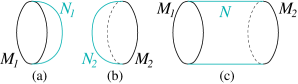
Figure 2: (Color online) Three space-time ${\cal M}_{1}$, ${\cal M}_{2}$, and ${\cal M}_{1}\sqcup-{\cal M}_{2}$, plus their extensions. ${\cal N}_{1}$, ${\cal N}_{2}$, and ${\cal N}$. The ratio of the action amplitudes (which are pure $U(1)$ phases) for space-time (a) and (b): $Z(a)/Z(b)=Z(a)Z^{*}(b)$ is given by the action amplitude for space-time (c): $Z(a)Z^{*}(b)=Z(c)$.

VIII.2 An exact evaluation of the partition function

Let us examine the action amplitude $\hskip 1.0pt\mathrm{e}^{\hskip 1.0pt\mathrm{i}\hskip 1.0pt2\pi\int_{{\cal M}^{d+1}}\phi_{M}^{*}\bar{\nu}_{d+1}+\hskip 1.0pt\mathrm{i}\hskip 1.0pt2\pi\int_{{\cal N}^{d+2}}\phi_{N}^{*}\bar{\omega}_{d+2}}$ for different $\phi_{M}$ but a fixed $\varphi$. $\phi_{N}$ is chosen such that it is given by $\varphi\phi_{M}$ at the boundary $\partial{\cal N}^{d+2}$. We know that $\varphi^{*}\bar{\omega}_{d+2}$ is a coboundary on $\partial{\cal N}^{d+2}$. Thus the value of $\hskip 1.0pt\mathrm{e}^{\hskip 1.0pt\mathrm{i}\hskip 1.0pt\pi\int_{{\cal N}^{d+2}}\phi_{N}^{*}\bar{\omega}_{d+2}}$ only depends $\phi_{N}$ on the boundary $\partial{\cal N}^{d+2}$, i.e. only depends on $\varphi\phi_{M}$. Therefore, the action amplitude $\hskip 1.0pt\mathrm{e}^{\hskip 1.0pt\mathrm{i}\hskip 1.0pt2\pi\int_{{\cal M}^{d+1}}\phi_{M}^{*}\bar{\nu}_{d+1}+\hskip 1.0pt\mathrm{i}\hskip 1.0pt2\pi\int_{{\cal N}^{d+2}}\phi_{N}^{*}\bar{\omega}_{d+2}}$ is a function of $\phi_{M}$.

Let us call $\phi_{M_{1}}:{\cal M}^{d+1}_{1}\to{\cal B}G_{fSO}$ and $\phi_{M_{2}}:{\cal M}^{d+1}_{2}\to{\cal B}G_{fSO}$ cobordant, if there exist a homomorphism $\varphi_{N}:{\cal N}^{d+2}\to{\cal B}G_{fSO}$ such that $\partial{\cal N}^{d+2}={\cal M}^{d+1}_{1}\sqcup{\cal M}^{d+1}_{2}$, $\varphi_{N}=\phi_{M_{1}}$ on the boundary ${\cal M}^{d+1}_{1}$, and $\varphi_{N}=\phi_{M_{2}}$ on the boundary ${\cal M}^{d+1}_{2}$ (see Fig. 2(c)). We can show that two cobordant $\phi_{M_{1}}$ and $\phi_{M_{2}}$ have the same action amplitude. This is because the difference (the ratio) of the action amplitudes is given by (see Fig. 2)

$$\hskip 1.0pt\mathrm{e}^{\hskip 1.0pt\mathrm{i}\hskip 1.0pt2\pi[\int_{{\cal M}^{d+1}_{1}}\phi_{M_{1}}^{*}\bar{\nu}_{d+1}-\int_{{\cal M}^{d+1}_{2}}\phi_{M_{2}}^{*}\bar{\nu}_{d+1}]+\hskip 1.0pt\mathrm{i}\hskip 1.0pt2\pi\int_{{\cal N}^{d+2}}\phi_{N}^{*}\bar{\omega}_{d+2}}$$ (68)

where $\phi_{N}=\varphi\varphi_{N}$. Because $\varphi_{N}=\phi_{M_{1}}$ or $\varphi_{N}=\phi_{M_{2}}$ on the two boundaries of ${\cal N}^{d+2}$, we have

$$\hskip 1.0pt\mathrm{e}^{\hskip 1.0pt\mathrm{i}\hskip 1.0pt2\pi[\int_{{\cal M}^{d+1}_{1}}\phi_{M_{1}}^{*}\bar{\nu}_{d+1}-\int_{{\cal M}^{d+1}_{2}}\phi_{M_{2}}^{*}\bar{\nu}_{d+1}]}$$

$$= \hskip 1.0pt\mathrm{e}^{\hskip 1.0pt\mathrm{i}\hskip 1.0pt2\pi[\int_{{\cal M}^{d+1}_{1}}\varphi_{N}^{*}\bar{\nu}_{d+1}-\int_{{\cal M}^{d+1}_{2}}\varphi_{N}^{*}\bar{\nu}_{d+1}]}$$

$$= \hskip 1.0pt\mathrm{e}^{\hskip 1.0pt\mathrm{i}\hskip 1.0pt2\pi\int_{{\cal N}^{d+2}}\hskip 1.0pt\mathrm{d}\varphi_{N}^{*}\bar{\nu}_{d+1}}$$ (69)

Now the difference (the ratio) of the action amplitudes is given by

$$\hskip 1.0pt\mathrm{e}^{\hskip 1.0pt\mathrm{i}\hskip 1.0pt2\pi\int_{{\cal N}^{d+2}}\hskip 1.0pt\mathrm{d}\varphi_{N}^{*}\bar{\nu}_{d+1}+\phi_{N}^{*}\bar{\omega}_{d+2}}$$

$$= \hskip 1.0pt\mathrm{e}^{\hskip 1.0pt\mathrm{i}\hskip 1.0pt2\pi\int_{{\cal N}^{d+2}}\hskip 1.0pt\mathrm{d}\varphi_{N}^{*}\bar{\nu}_{d+1}+\varphi_{N}^{*}\varphi^{*}\bar{\omega}_{d+2}}$$

$$= \hskip 1.0pt\mathrm{e}^{\hskip 1.0pt\mathrm{i}\hskip 1.0pt2\pi\int_{{\cal N}^{d+2}}\varphi_{N}^{*}(\hskip 1.0pt\mathrm{d}\bar{\nu}_{d+1}+\varphi^{*}\bar{\omega}_{d+2})}=1.$$ (70)

We like to remark that in the action amplitude $\hskip 1.0pt\mathrm{e}^{\hskip 1.0pt\mathrm{i}\hskip 1.0pt2\pi\int_{{\cal M}^{d+1}}\phi_{M}^{*}\bar{\nu}_{d+1}+\hskip 1.0pt\mathrm{i}\hskip 1.0pt2\pi\int_{{\cal N}^{d+2}}\phi_{N}^{*}\bar{\omega}_{d+2}}$, the homomorphism $\phi_{M}:{\cal M}^{d+1}\to{\cal B}G_{fSO}$ usually cannot be extended to a homomorphism $\varphi_{N}:{\cal N}^{d+2}\to{\cal B}G_{fSO}$ (i.e. $\phi_{M}$ is not cobordant to a trivial homomorphism). As a result the action amplitude is not equal to 1. If the homomorphism $\phi_{M}:{\cal M}^{d+1}\to{\cal B}G_{fSO}$ can be extend to ${\cal N}^{d+2}$, the action amplitude will be equal to one. If $\phi_{M_{1}}$ and $\phi_{M_{2}}$ are cobordant, then $\phi_{M_{1}}$ and $\phi_{M_{2}}$ on ${\cal M}_{1}$ and ${\cal M}_{2}$ in Fig. 2(c) can be extended to ${\cal N}$. In this case, the action amplitude for space-time Fig. 2(c) will be equal to one.

In our exactly soluble model (VIII.1), the homomorphism $\phi_{M}$ is determined by $a^{G_{fSO}}$ which in turn is given by the dynamical fields $g_{i}$ on vertices and the background field $A^{G_{fSO}}$ in the links (see eqn. (59)). For a fixed $A^{G_{fSO}}$, the different homomorphisms $\phi_{M}$ are all cobordant to each other, and the corresponding action amplitudes are all equal to each other. Therefore, the partition function for our model (VIII.1) can be calculated exactly

$$Z({\cal M}^{d+1},A^{G_{fSO}})=\sum_{\phi_{M}}\hskip 1.0pt\mathrm{e}^{\hskip 1.0pt\mathrm{i}\hskip 1.0pt2\pi\big{(}\int_{{\cal M}^{d+1}}\phi_{M}^{*}\bar{\nu}_{d+1}+\int_{{\cal N}^{d+2}}\phi_{N}^{*}\bar{\omega}_{d+2}\big{)}}$$

$$=V^{N_{v}}\hskip 1.0pt\mathrm{e}^{\hskip 1.0pt\mathrm{i}\hskip 1.0pt2\pi\int_{{\cal M}^{d+1}}\nu_{d+1}(A^{G_{fSO}})+\hskip 1.0pt\mathrm{i}\hskip 1.0pt\pi\int_{{\cal N}^{d+2}}\text{Sq}^{2}f_{d}+f_{d}{\rm w}_{2}}$$ (71)

where $V$ is the volume of $G_{fSO}$ and $N_{v}$ the number of vertices in ${\cal M}^{d+1}$. We see that the fermionic SPT state realized by (VIII.1) [which is labeled by a pair $(\varphi,\bar{\nu}_{d+1})$] is characterized by the SPT invariant

$$Z^{\text{top}}({\cal M}^{d+1},A^{G_{fSO}})$$

$$= \hskip 1.0pt\mathrm{e}^{\hskip 1.0pt\mathrm{i}\hskip 1.0pt2\pi\int_{{\cal M}^{d+1}}\nu_{d+1}(A^{G_{fSO}})+\hskip 1.0pt\mathrm{i}\hskip 1.0pt\pi\int_{{\cal N}^{d+2}}\text{Sq}^{2}f_{d}+f_{d}{\rm w}_{2}},$$ (72)

where $f_{d}\overset{\scriptscriptstyle 2}{=}n_{d}(A^{G_{fSO}})$ on $\partial{\cal N}^{d+2}$ and

$$-\hskip 1.0pt\mathrm{d}\nu_{d+1}(A^{G_{fSO}}) \overset{\scriptscriptstyle 1}{=}\frac{1}{2}\text{Sq}^{2}n_{d}(A^{G_{fSO}})$$

$$+\frac{1}{2}n_{d}(A^{G_{fSO}}){\rm w}_{2}(A^{SO}).$$ (73)

Here $A^{SO}_{ij}=\pi(A^{G_{fSO}}_{ij})\in SO_{\infty}$ and $A^{SO}$ must be the connection for the tangent bundle on ${\cal M}^{d+1}$.

Eqn. (VIII.2) can also be rewritten as

$$Z^{\text{top}}({\cal M}^{d+1},A^{G_{fSO}})$$

$$= \hskip 1.0pt\mathrm{e}^{\hskip 1.0pt\mathrm{i}\hskip 1.0pt2\pi\int_{{\cal M}^{d+1}}\phi_{M}^{*}\bar{\nu}_{d+1}+\hskip 1.0pt\mathrm{i}\hskip 1.0pt2\pi\int_{{\cal N}^{d+2}}\phi_{N}^{*}\bar{\omega}_{d+2}},$$

$$\phi_{N}|_{\partial{\cal N}^{d+2}}=\varphi\phi_{M},$$ (74)

where the homomorphism $\phi_{M}:{\cal M}^{d+1}\to{\cal B}G_{fSO}$ is determined by the background field $A^{G_{fSO}}$ via

$$A^{G_{fSO}}=\phi_{M}^{*}\bar{a}^{G_{fSO}}.$$ (75)

Also $\phi_{N}$ is a homomorphism $\phi_{N}:{\cal N}^{d+2}\to{\cal B}_{f}(SO_{\infty},1;\mathbb{Z}_{2},d)$, such that, on the boundary ${\cal M}^{d+1}=\partial{\cal N}^{d+2}$, $\phi_{N}$ is given by $\varphi\phi_{M}$, where $\varphi$ is a homomorphism $\varphi:{\cal B}G_{fSO}\to{\cal B}_{f}(SO_{\infty},1;\mathbb{Z}_{2},d)$.

VIII.3 Equivalent relations between the labels $(\varphi,\bar{\nu}_{d+1})$

It is possible that the SPT states labeled by different pairs $(\varphi,\bar{\nu}_{d+1})$ and $(\varphi^{\prime},\bar{\nu}_{d+1}^{\prime})$, i.e. by different pairs $[n_{d}(A^{G_{fSO}}),\nu_{d+1}(A^{G_{fSO}})]$ and $[n_{d}^{\prime}(A^{G_{fSO}}),\nu_{d+1}^{\prime}(A^{G_{fSO}})]$, are the same SPT states since the two pair may give rise to the same SPT invariant. In this case, we say that the two pairs are equivalent.

What are the equivalent relations for the pairs $(\varphi,\bar{\nu}_{d+1})$ or $[n_{d}(A^{G_{fSO}}),\nu_{d+1}(A^{G_{fSO}})]$? Here is our proposal: $(\varphi,\bar{\nu}_{d+1})$ and $(\varphi^{\prime},\bar{\nu}_{d+1}^{\prime})$ are equivalent if

1. There exists a $\mathbb{R}/\mathbb{Z}$-valued $d+2$-cocycle $\bar{\Omega}_{d+2}$ on $I\times{\cal B}_{f}(SO_{\infty},1;Z_{2},d)$ such that when restricted on the two boundaries of $I\times{\cal B}_{f}(SO_{\infty},1;Z_{2},d)$, $\bar{\Omega}_{d+2}$ becomes $\bar{\omega}_{d+2}$ in eqn. (91).

2. There exists a homomorphism $\Phi:I\times{\cal B}G_{fSO}\to I\times{\cal B}_{f}(SO_{\infty},1;Z_{2},d)$ such that on the two boundaries, $\Phi$ reduces to $\varphi$ and $\varphi^{\prime}$.

3. There exists a $\mathbb{R}/\mathbb{Z}$-valued $d+1$-cochain $\bar{\mu}_{d+1}$ on $I\times{\cal B}G_{fSO}$ such that $-\hskip 1.0pt\mathrm{d}\bar{\mu}_{d+1}\overset{\scriptscriptstyle 1}{=}\Phi^{*}\bar{\Omega}_{d+2}$ and $\bar{\mu}_{d+1}$ reduces to $\bar{\nu}_{d+1}$ and $\bar{\nu}_{d+1}^{\prime}$ on the two boundaries.

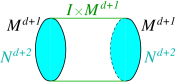
Figure 3: (Color online) The boundary of $I\times{\cal N}^{d+2}$ is given by ${\cal N}^{d+2}\sqcup I\times{\cal M}^{d+1}\sqcup{\cal N}^{d+2}$. The boundary of $I\times{\cal M}^{d+1}$ is given by ${\cal M}^{d+1}\sqcup{\cal M}^{d+1}$.

In the following, we like to show that equivalent $(\varphi,\bar{\nu}_{d+1})$ and $(\varphi^{\prime},\bar{\nu}_{d+1}^{\prime})$ give rise to the same SPT invariant (VIII.2), and hence the same SPT order. Since $\hskip 1.0pt\mathrm{d}\bar{\Omega}_{d+2}\overset{\scriptscriptstyle 1}{=}0$, we have (see Fig. 3)

$$1= \hskip 1.0pt\mathrm{e}^{\hskip 1.0pt\mathrm{i}\hskip 1.0pt2\pi\int_{I\times{\cal N}^{d+2}}\tilde{\phi}_{N}^{*}\hskip 1.0pt\mathrm{d}{\bar{\Omega}}_{d+2}}=\hskip 1.0pt\mathrm{e}^{\hskip 1.0pt\mathrm{i}\hskip 1.0pt2\pi\int_{I\times{\cal M}^{d+2}}\tilde{\phi}_{N}^{*}\bar{\Omega}_{d+2}}\times$$

$$\hskip 1.0pt\mathrm{e}^{-\hskip 1.0pt\mathrm{i}\hskip 1.0pt2\pi\int_{{\cal N}^{d+2}}\phi_{N}^{*}\bar{\omega}_{d+2}}\hskip 1.0pt\mathrm{e}^{+\hskip 1.0pt\mathrm{i}\hskip 1.0pt2\pi\int_{{\cal N}^{d+2}}(\phi_{N}^{\prime})^{*}\bar{\omega}_{d+2}},$$ (76)

where $\tilde{\phi}_{N}$ is a homomorphism $\tilde{\phi}_{N}:I\times{\cal N}^{d+2}\to I\times{\cal B}_{f}(SO_{\infty},1;Z_{2},d)$ such that on the two boundaries $\tilde{\phi}_{N}$ is given by $\phi_{N}:{\cal N}^{d+2}\to{\cal B}_{f}(SO_{\infty},1;Z_{2},d)$ and $\phi_{N}^{\prime}:{\cal N}^{d+2}\to{\cal B}_{f}(SO_{\infty},1;Z_{2},d)$.

We choose $\tilde{\phi}_{N}$ such that on the boundary of ${\cal N}^{d+2}$, $\phi_{N}$ becomes $\varphi\phi_{M}:{\cal M}^{d+1}\to{\cal B}_{f}(SO_{\infty},1;Z_{2},d)$ and $\phi_{N}^{\prime}$ becomes $\varphi^{\prime}\phi_{M}:{\cal M}^{d+1}\to{\cal B}_{f}(SO_{\infty},1;Z_{2},d)$, where $\phi_{M}$ is a homomorphisms $\phi_{M}:{\cal M}^{d+1}\to{\cal B}G_{fSO}$, and $\varphi$ and $\varphi^{\prime}$ are the homomorphisms $\varphi:{\cal B}G_{fSO}\to{\cal B}_{f}(SO_{\infty},1;Z_{2},d)$ and $\varphi^{\prime}:{\cal B}G_{fSO}\to{\cal B}_{f}(SO_{\infty},1;Z_{2},d)$. We note that $\phi_{M}$ determines the background field $A^{G_{fSO}}$. Similarly, on the two boundaries of $I\times{\cal M}^{d+1}$, $\tilde{\phi}_{N}$ is also given by $\varphi\phi_{M}$ and $\varphi^{\prime}\phi_{M}$.

Since $\varphi$ and $\varphi^{\prime}$ are given by $\Phi:I\times{\cal B}G_{fSO}\to I\times{\cal B}_{f}(SO_{\infty},1;Z_{2},d)$ when restricted on the two boundaries, therefore we can choose $\tilde{\phi}_{N}$ such that on $I\times{\cal M}^{d+1}$, $\tilde{\phi}_{N}$ is given by $\Phi\tilde{\phi}_{M}$ where $\tilde{\phi}_{M}$ is a homomorphism $\tilde{\phi}_{M}:I\times{\cal M}^{d+1}\to I\times{\cal B}G_{fSO}$. Now, we find (see Fig. 3)

$$\hskip 1.0pt\mathrm{e}^{\hskip 1.0pt\mathrm{i}\hskip 1.0pt2\pi\int_{I\times{\cal M}^{d+2}}\tilde{\phi}_{N}^{*}\bar{\Omega}_{d+2}}=\hskip 1.0pt\mathrm{e}^{\hskip 1.0pt\mathrm{i}\hskip 1.0pt2\pi\int_{I\times{\cal M}^{d+1}}\tilde{\phi}_{M}^{*}\Phi^{*}\bar{\Omega}_{d+2}}$$

$$= \hskip 1.0pt\mathrm{e}^{-\hskip 1.0pt\mathrm{i}\hskip 1.0pt2\pi\int_{I\times{\cal M}^{d+1}}\tilde{\phi}_{M}^{*}\hskip 1.0pt\mathrm{d}\bar{\mu}_{d+1}}$$

$$= \hskip 1.0pt\mathrm{e}^{-\hskip 1.0pt\mathrm{i}\hskip 1.0pt2\pi\int_{{\cal M}^{d+1}}\phi_{M}^{*}\bar{\nu}_{d+1}-\phi_{M}^{*}\bar{\nu}_{d+1}^{\prime}}$$ (77)

The above reduces eqn. (VIII.3) to

$$1= \hskip 1.0pt\mathrm{e}^{-\hskip 1.0pt\mathrm{i}\hskip 1.0pt2\pi\int_{{\cal M}^{d+1}}\phi_{M}^{*}\bar{\nu}_{d+1}-\phi_{M}^{*}\bar{\nu}_{d+1}^{\prime}}\times$$

$$\hskip 1.0pt\mathrm{e}^{-\hskip 1.0pt\mathrm{i}\hskip 1.0pt2\pi\int_{{\cal N}^{d+2}}\phi_{N}^{*}\bar{\omega}_{d+2}}\hskip 1.0pt\mathrm{e}^{+\hskip 1.0pt\mathrm{i}\hskip 1.0pt2\pi\int_{{\cal N}^{d+2}}(\phi_{N}^{\prime})^{*}\bar{\omega}_{d+2}},$$ (78)

which complete our proof (see eqn. (VIII.2)).

The fermionic SPT states can also be labeled by $[\bar{n}_{d}(\bar{a}^{G_{fSO}}),\bar{\nu}_{d+1}(\bar{a}^{G_{fSO}})]$ where $\bar{n}_{d}(\bar{a}^{G_{fSO}})$ is a $\mathbb{Z}_{2}$-valued $d$-cocycle and $\bar{\nu}_{d+1}(\bar{a}^{G_{fSO}})$ is a $\mathbb{R}/\mathbb{Z}$-valued $d+1$-cochian on ${\cal B}G_{fSO}$. They are functions of canonical cocycle $\bar{a}^{G_{fSO}}$ on ${\cal B}G_{fSO}$. In terms of $[\bar{n}_{d}(\bar{a}^{G_{fSO}}),\bar{\nu}_{d+1}(\bar{a}^{G_{fSO}})]$, the equivalence relations are particially generated by the following two transformations (see eqn. (276)):

1. Transformation generated by $d$-cohain $\bar{\eta}_{d}(\bar{a}^{G_{fSO}})\in C^{d-1}({\cal B}G_{fSO};\mathbb{R}/\mathbb{Z})$

   $$\bar{n}_{d}(\bar{a}^{G_{fSO}})\to \bar{n}_{d}(\bar{a}^{G_{fSO}})$$

   $$\bar{\nu}_{d+1}(\bar{a}^{G_{fSO}})\to \bar{\nu}_{d+1}(\bar{a}^{G_{fSO}})+\hskip 1.0pt\mathrm{d}\bar{\eta}_{d}(\bar{a}^{G_{fSO}}).$$ (79)

2. Transformation generated by $d-1$-cohain $\bar{u}_{d}\in C^{d-1}({\cal B}G_{fSO};\mathbb{Z}_{2})$

   $$\bar{n}_{d}(\bar{a}^{G_{fSO}})\to\bar{n}_{d}(\bar{a}^{G_{fSO}})+\hskip 1.0pt\mathrm{d}\bar{u}_{d-1}(\bar{a}^{G_{fSO}})$$ (80)

   $$\bar{\nu}_{d+1}(\bar{a}^{G_{fSO}})\to\bar{\nu}_{d+1}(\bar{a}^{G_{fSO}})+\frac{1}{2}\bar{u}_{d-1}(\bar{a}^{G_{fSO}})\bar{\rm w}_{2}(\bar{a}^{SO})$$

   $$+\frac{1}{2}\mathbb{Sq}^{2}\bar{u}_{d-1}(\bar{a}^{G_{fSO}})+\frac{1}{2}\hskip 1.0pt\mathrm{d}\bar{u}_{d-1}(\bar{a}^{G_{fSO}})\underset{{\scriptscriptstyle d-1}}{\smile}\bar{n}_{d}(\bar{a}^{G_{fSO}}).$$

We can show the above two transformation generate equivalent relations since they do not change the SPT invariant (VIII.2).

In fact, we have a more general equivalent relation in terms of $[n_{d}(a^{G_{fSO}}),\nu_{d+1}(a^{G_{fSO}})]$ in eqn. (VII.2). Here $n_{d}(a^{G_{fSO}})=\phi_{M}^{*}\bar{n}_{d}(\bar{a}^{G_{fSO}})$ and $\nu_{d+1}(a^{G_{fSO}})=\phi_{M}^{*}\bar{\nu}_{d+1}(\bar{a}^{G_{fSO}})$ are a $d$-cocycle and a $d+1$-cochain on space-time ${\cal M}^{d+1}$. $[n_{d}(a^{G_{fSO}}),\nu_{d+1}(a^{G_{fSO}})]$ and $[n_{d}^{\prime}(a^{G_{fSO}}),\nu_{d+1}^{\prime}(a^{G_{fSO}})]$ produce the same SPT invariant if they satisfy (see eqn. (276)):

1. Equivalence relation generated by $d$-cohain $\eta_{d}\in C^{d-1}({\cal M}^{d+1};\mathbb{R}/\mathbb{Z})$

   $$n_{d}^{\prime}(a^{G_{fSO}})\overset{\scriptscriptstyle 2}{=} n_{d}(a^{G_{fSO}})$$

   $$\nu_{d+1}^{\prime}(a^{G_{fSO}})\overset{\scriptscriptstyle 1}{=} \nu_{d+1}(a^{G_{fSO}})+\hskip 1.0pt\mathrm{d}\eta_{d}.$$ (81)

2. Equivalence relation generated by $d-1$-cohain $u_{d}\in C^{d-1}({\cal M}^{d+1};\mathbb{Z}_{2})$

   $$n_{d}^{\prime}(a^{G_{fSO}})\overset{\scriptscriptstyle 2}{=}n_{d}(a^{G_{fSO}})+\hskip 1.0pt\mathrm{d}u_{d-1}$$ (82)

   $$\nu_{d+1}^{\prime}(a^{G_{fSO}})\overset{\scriptscriptstyle 1}{=}\nu_{d+1}(a^{G_{fSO}})+\frac{1}{2}u_{d-1}{\rm w}_{2}(a^{SO})$$

   $$+\frac{1}{2}\mathbb{Sq}^{2}u_{d-1}+\frac{1}{2}\hskip 1.0pt\mathrm{d}u_{d-1}\underset{{\scriptscriptstyle d-1}}{\smile}n_{d}(a^{G_{fSO}}).$$

Because $u_{d-1}$ and $\eta_{d}$ are cochains on ${\cal M}^{d+1}$, which do not have to be the pullbacks of cochains $\bar{u}_{d-1}(\bar{a}^{G_{fSO}})$ and $\bar{\eta}_{d-1}(\bar{a}^{G_{fSO}})$ on ${\cal B}G_{fSO}$. So the above equivalent relation is more general.

Using a similar method (see Fig. 3), we can show that above $[n_{d}(a^{G_{fSO}}),\nu_{d+1}(a^{G_{fSO}})]$ and $[n_{d}^{\prime}(a^{G_{fSO}}),\nu_{d+1}^{\prime}(a^{G_{fSO}})]$ produce the same action amplitude (thus the same SPT invariant). So the above relations are indeed equivalent relations.

We first introduce a $\mathbb{Z}_{2}$-valued cochain $\Omega_{d+2}$ on $I\times{\cal N}^{d+2}$

$$\Omega_{d+2}\overset{\scriptscriptstyle 1}{=}\frac{1}{2}\mathbb{Sq}^{2}F_{d}+\frac{1}{2}F_{d}{\rm w}_{2}$$ (83)

where $F_{d}$ is a $\mathbb{Z}_{2}$-valued cocycle on $I\times{\cal N}^{d+2}$ given by

$$F_{d}=f_{d}+\hskip 1.0pt\mathrm{d}U_{d-1}$$ (84)

and $U_{d-1}$ is a $\mathbb{Z}_{2}$-valued cochain on $I\times{\cal N}^{d+2}$. We know that the boundary of $I\times{\cal N}^{d+2}$ has three pieces ${\cal N}^{d+2}$, $I\times{\cal M}^{d+1}$ and ${\cal N}^{d+2}$. $U_{d-1}$ is chosen such that it becomes $0$ on one of the ${\cal N}^{d+2}$, and becomes $u_{d-1}$ on the boundary of the second ${\cal N}^{d+2}$: ${\cal M}^{d+1}=\partial{\cal N}^{d+2}$. Using eqn. (273), we see that $\Omega_{d+2}$ is actually a cocycle on $I\times{\cal N}^{d+2}$. Therefore, we have (see Fig. 3)

$$1= \hskip 1.0pt\mathrm{e}^{\hskip 1.0pt\mathrm{i}\hskip 1.0pt2\pi\int_{I\times{\cal N}^{d+2}}\hskip 1.0pt\mathrm{d}\Omega_{d+2}}=\hskip 1.0pt\mathrm{e}^{\hskip 1.0pt\mathrm{i}\hskip 1.0pt\pi\int_{I\times{\cal M}^{d+2}}\mathbb{Sq}^{2}F_{d}+F_{d}{\rm w}_{2}}\times$$

$$\hskip 1.0pt\mathrm{e}^{-\hskip 1.0pt\mathrm{i}\hskip 1.0pt\pi\int_{{\cal N}^{d+2}}\text{Sq}^{2}f_{d}+f_{d}{\rm w}_{2}}\hskip 1.0pt\mathrm{e}^{+\hskip 1.0pt\mathrm{i}\hskip 1.0pt\pi\int_{{\cal N}^{d+2}}\text{Sq}^{2}f_{d}^{\prime}+f_{d}^{\prime}{\rm w}_{2}},$$ (85)

where $f_{d}^{\prime}\overset{\scriptscriptstyle 2}{=}f_{d}+\hskip 1.0pt\mathrm{d}U_{d-1}$ on ${\cal N}^{d+2}$. On the boundary ${\cal M}^{d+1}=\partial{\cal N}^{d+2}$, $f_{d}^{\prime}\overset{\scriptscriptstyle 2}{=}f_{d}+\hskip 1.0pt\mathrm{d}U_{d-1}$ becomes $n_{d}^{\prime}\overset{\scriptscriptstyle 2}{=}n_{d}+\hskip 1.0pt\mathrm{d}u_{d-1}$ (see eqn. (80)).

Next we calculate $\hskip 1.0pt\mathrm{e}^{\hskip 1.0pt\mathrm{i}\hskip 1.0pt\pi\int_{I\times{\cal M}^{d+2}}\mathbb{Sq}^{2}F_{d}+F_{d}{\rm w}_{2}}$ (using eqn. (276)):

$$\ \ \ \ \hskip 1.0pt\mathrm{e}^{\hskip 1.0pt\mathrm{i}\hskip 1.0pt\pi\int_{I\times{\cal M}^{d+2}}\mathbb{Sq}^{2}(f_{d}+\hskip 1.0pt\mathrm{d}U_{d-1})+(f_{d}+\hskip 1.0pt\mathrm{d}U_{d-1}){\rm w}_{2}}$$

$$=\hskip 1.0pt\mathrm{e}^{\hskip 1.0pt\mathrm{i}\hskip 1.0pt\pi\int_{I\times{\cal M}^{d+2}}\text{Sq}^{2}f_{d}+f_{d}{\rm w}_{2}+\hskip 1.0pt\mathrm{d}\big{(}\mathbb{Sq}^{2}U_{d-1}+\hskip 1.0pt\mathrm{d}U_{d-1}\underset{{\scriptscriptstyle d-1}}{\smile}n_{d}+U_{d-1}{\rm w}_{2}\big{)}}$$

$$=\hskip 1.0pt\mathrm{e}^{\hskip 1.0pt\mathrm{i}\hskip 1.0pt2\pi\int_{I\times{\cal M}^{d+2}}\hskip 1.0pt\mathrm{d}\big{(}\nu_{d+1}+\frac{1}{2}\mathbb{Sq}^{2}U_{d-1}+\frac{1}{2}\hskip 1.0pt\mathrm{d}U_{d-1}\underset{{\scriptscriptstyle d-1}}{\smile}n_{d}+\frac{1}{2}U_{d-1}{\rm w}_{2}\big{)}}$$

$$=\hskip 1.0pt\mathrm{e}^{\hskip 1.0pt\mathrm{i}\hskip 1.0pt2\pi\int_{{\cal M}^{d+2}}\nu_{d+1}}\hskip 1.0pt\mathrm{e}^{-\hskip 1.0pt\mathrm{i}\hskip 1.0pt2\pi\int_{{\cal M}^{d+2}}\nu_{d+1}^{\prime}}$$ (86)

Combined with eqn. (VIII.3), we find

$$\ \ \ \ \hskip 1.0pt\mathrm{e}^{\hskip 1.0pt\mathrm{i}\hskip 1.0pt2\pi\int_{{\cal M}^{d+2}}\nu_{d+1}+\hskip 1.0pt\mathrm{i}\hskip 1.0pt\pi\int_{{\cal N}^{d+2}}\text{Sq}^{2}f_{d}+f_{d}{\rm w}_{2}}$$

$$=\hskip 1.0pt\mathrm{e}^{\hskip 1.0pt\mathrm{i}\hskip 1.0pt2\pi\int_{{\cal M}^{d+2}}\nu_{d+1}^{\prime}+\hskip 1.0pt\mathrm{i}\hskip 1.0pt\pi\int_{{\cal N}^{d+2}}\text{Sq}^{2}f_{d}^{\prime}+f_{d}^{\prime}{\rm w}_{2}}$$ (87)

The action amplitudes are indeed the same.

We like to remark that $[n_{d}(a^{G_{fSO}}),\nu_{d+1}(a^{G_{fSO}})]$ and $[n_{d}^{\prime}(a^{G_{fSO}}),\nu_{d+1}^{\prime}(a^{G_{fSO}})]$ not related by the above two types of transformations may still describe the same SPT phase. To really show $[n_{d}(a^{G_{fSO}}),\nu_{d+1}(a^{G_{fSO}})]$ and $[n_{d}^{\prime}(a^{G_{fSO}}),\nu_{d+1}^{\prime}(a^{G_{fSO}})]$ describe different SPT phases, we need to show they produce different SPT invariants.

VIII.4 Stacking and Abelian group structure of fermionic SPT phases

We have seen that the higher dimensional bosonization is closely related to a higher group ${\cal B}_{f}(SO_{\infty},1;Z_{2},d)$, and a particular choice of a ${\mathbb{R}/\mathbb{Z}}$-valued cocycle $\frac{1}{2}\text{Sq}^{2}\bar{f}_{d}+\frac{1}{2}\bar{f}_{d}\bar{\rm w}_{2}$ on the higher group. Such a choice of cocycle has an important additive property

$$\ \ \ \ \frac{1}{2}\text{Sq}^{2}(\bar{f}_{d}+\bar{f}_{d}^{\prime})+\frac{1}{2}(\bar{f}_{d}+\bar{f}_{d}^{\prime})\bar{\rm w}_{2}$$

$$\overset{\scriptscriptstyle 1,\hskip 1.0pt\mathrm{d}}{=}\Big{(}\frac{1}{2}\text{Sq}^{2}\bar{f}_{d}+\frac{1}{2}\bar{f}_{d}\bar{\rm w}_{2}\Big{)}+\Big{(}\frac{1}{2}\text{Sq}^{2}\bar{f}_{d}^{\prime}+\frac{1}{2}\bar{f}_{d}^{\prime}\bar{\rm w}_{2}\Big{)}.$$ (88)

This additive property insure that the fermionic SPT phases can also be added so that the collection of fermionic SPT phases actually form an Abelian group. The addition of two SPT states physically corresponds to stacking two SPT states one on top another, which implies that the SPT phases should always have an Abelian group structure.

For two SPT phases described by $(\bar{n}_{d},\bar{\nu}_{d+1})$ and $(\bar{n}_{d}^{\prime},\bar{\nu}_{d+1}^{\prime})$, they add following a twisted addition rule

$$(\bar{n}_{d},\bar{\nu}_{d+1})+(\bar{n}_{d}^{\prime},\bar{\nu}_{d+1}^{\prime})$$

$$= (\bar{n}_{d}+\bar{n}_{d}^{\prime},\bar{\nu}_{d+1}+\bar{\nu}_{d+1}^{\prime}+\frac{1}{2}\bar{n}_{d}\underset{{\scriptscriptstyle d-1}}{\smile}\bar{n}_{d}^{\prime}).$$ (89)

This allows us to extract the group $\text{fSPT}_{d+1}(G_{fSO})$ given by the stacking of fermionic SPTs with symmetry $G^{f}$. Clearly there is homomorphism

$$\text{fSPT}_{d+1}(G_{fSO}) \to H^{d}({\cal B}G_{fSO};\mathbb{Z}_{2})$$

$$(\bar{n}_{d},\nu_{d+1}) \mapsto\bar{n}_{d}.$$

Not every $\bar{n}_{d}$ allows a solution of $\bar{\nu}_{d+1}$; the image of the above homomorphism is a subgroup of $H^{d}({\cal B}G_{fSO};\mathbb{Z}_{2})$, which will be called the obstruction-free subgroup, denoted by $BH^{d}({\cal B}G_{fSO};\mathbb{Z}_{2})$. The kernel of the above homomorphism is a quotient group of $H^{d+1}({\cal B}G_{fSO};{\mathbb{R}/\mathbb{Z}})$. This is because of the extra gauge transformation $\frac{1}{2}(\mathbb{Sq}^{2}\bar{u}_{d-1}+\bar{u}_{d-1}{\rm w}_{2})$ when $\bar{n}_{d}=0$. Let $\Gamma\subset H^{d+1}({\cal B}G_{fSO};{\mathbb{R}/\mathbb{Z}})$ be the subgroup generated by $\frac{1}{2}(\mathbb{Sq}^{2}\bar{u}_{d-1}+\bar{u}_{d-1}\bar{\rm w}_{2}),\forall\bar{u}_{d-1}\in{\cal C}^{d-1}({\cal B}G_{fSO};\mathbb{Z}_{2})$, we have the following exact sequence for group extension:

$$H^{d+1}({\cal B}G_{fSO};{\mathbb{R}/\mathbb{Z}})/\Gamma \to\text{fSPT}_{d+1}(G_{fSO})$$

$$\to BH^{d+1}({\cal B}G_{fSO};\mathbb{Z}_{2}),$$ (90)

whose corresponding group 2-cocycle in $H^{2}[BH^{d}({\cal B}G_{fSO};\mathbb{Z}_{2}),H^{d+1}({\cal B}G_{fSO};{\mathbb{R}/\mathbb{Z}})/\Gamma]$ is given by $\frac{1}{2}\bar{n}_{d}\underset{{\scriptscriptstyle d-1}}{\smile}\bar{n}_{d}^{\prime}$.

We know that bosonic topological orders form a commutative monoid under the stacking operation $\boxtimes$ Kong and Wen (2014). However, For bosonic topological order with emergent fermions, they cannot have inverse for the stacking operation $\boxtimes$, and thus they are not invertible topological orders Kong and Wen (2014); Freed (2014); Kapustin (2014a); Freed and Hopkins (2016). However, we may modify the stacking operation by allowing the pairs of fermions from the two stacked phases to condense (equivalently, identifying fermions from the two stacked phases). Such a modified stacking operation is discussed in detail in LABEL:LW160205936,LW160205946. We denote the modified stacking operation by $\boxtimes_{f}$. The fermionic SPT states form an Abelian group under the modified stacking operation $\boxtimes_{f}$, as in eqn. (VIII.4).

VIII.5 With time reversal symmetry

In the above, we discussed the situation without time-reversal symmetry. In the presence of time reversal symmetry, we have the following result. The exactly soluble model (56) and the related fermionic SPT state is characterized by the following data:

1. A particular higher group ${\cal B}_{f}(O_{\infty},1;Z_{2},d)$, determined by its $\mathbb{Z}_{2}$-valued canonical cochain $\hskip 1.0pt\mathrm{d}\bar{f}_{d}\overset{\scriptscriptstyle 2}{=}0$ (see LABEL:ZLW and Appendix L).

2. A particular ${\mathbb{R}/\mathbb{Z}}$-valued $d+2$-cocycle on

   $$\bar{\omega}_{d+2}\overset{\scriptscriptstyle 1}{=}\frac{1}{2}\text{Sq}^{2}\bar{f}_{d}+\frac{1}{2}\bar{f}_{d}[\bar{\rm w}_{2}(\bar{a}^{O})+\bar{\rm w}_{1}^{2}(\bar{a}^{O})]$$ (91)

   on ${\cal B}_{f}(O_{\infty},1;Z_{2},d)$.

3. Different trivialization homomorphisms $\varphi:{\cal B}G_{fO}\to{\cal B}_{f}(O_{\infty},1;Z_{2},d)$, where $G_{fO}=G_{f}\leftthreetimes O_{\infty}$.

4. Different choices of the trivialization $\nu_{d+1}(\bar{a}^{G_{fO}})$ that satisfy $-\hskip 1.0pt\mathrm{d}\nu_{d+1}(\bar{a}^{G_{fO}})\overset{\scriptscriptstyle 1}{=}\varphi^{*}\bar{\omega}_{d+2}(\bar{f}_{d},\bar{a}^{O})$.

We like remark that in the above, the time reversal symmetry in $O_{\infty}$ acts non-trivially on the value of $\nu_{d+1}$ (see Appendix A).

We can also use $[\bar{n}_{d}(\bar{a}^{G_{fO}}),\bar{\nu}_{d+1}(\bar{a}^{G_{fO}})]$ in eqn. (VII.1) to label the fermion SPT states with time reversal symmetry. The equivalence relations are partially generated by the following two relations (see eqn. (276)):

1. Equivalence relation generated by $d$-cohain $\bar{\eta}_{d}\in C^{d-1}({\cal B}G_{fSO};\mathbb{R}/\mathbb{Z})$

   $$\bar{n}_{d}^{\prime}(\bar{a}^{G_{fO}})\overset{\scriptscriptstyle 2}{=} \bar{n}_{d}(\bar{a}^{G_{fO}})$$

   $$\bar{\nu}_{d+1}(\bar{a}^{G_{fO}})\overset{\scriptscriptstyle 1}{=} \bar{\nu}_{d+1}^{\prime}(\bar{a}^{G_{fO}})+\hskip 1.0pt\mathrm{d}\bar{\eta}_{d}(\bar{a}^{G_{fO}})$$ (92)

2. Equivalence relation generated by $d-1$-cohain $\bar{u}_{d-1}\in C^{d-1}({\cal B}G_{fSO};\mathbb{Z}_{2})$

   $$\bar{n}_{d}^{\prime}(\bar{a}^{G_{fO}})\overset{\scriptscriptstyle 2}{=}\bar{n}_{d}(\bar{a}^{G_{fO}})+\hskip 1.0pt\mathrm{d}\bar{u}_{d-1}(\bar{a}^{G_{fO}})$$ (93)

   $$\bar{\nu}_{d+1}^{\prime}(\bar{a}^{G_{fO}})\overset{\scriptscriptstyle 1}{=}\bar{\nu}_{d+1}(\bar{a}^{G_{fO}})+\frac{1}{2}\hskip 1.0pt\mathrm{d}\bar{u}_{d-1}(\bar{a}^{G_{fO}})\underset{{\scriptscriptstyle d-1}}{\smile}\bar{n}_{d}(\bar{a}^{G_{fO}})$$

   $$+\frac{1}{2}\mathbb{Sq}^{2}\bar{u}_{d-1}(\bar{a}^{G_{fO}})+\frac{1}{2}\bar{u}_{d-1}(\bar{a}^{G_{fO}})[\bar{\rm w}_{2}(a^{O})+\bar{\rm w}_{1}^{2}(a^{O})]$$

The corresponding SPT invariant is given by

$$Z^{\text{top}}({\cal M}^{d+1},A^{G_{fO}})$$

$$= \hskip 1.0pt\mathrm{e}^{\hskip 1.0pt\mathrm{i}\hskip 1.0pt2\pi\int_{{\cal M}^{d+1}}\nu_{d+1}(A^{G_{fO}})+\hskip 1.0pt\mathrm{i}\hskip 1.0pt\pi\int_{{\cal N}^{d+2}}\text{Sq}^{2}f_{d}+f_{d}({\rm w}_{2}+{\rm w}_{1}^{2})},$$

$$= \hskip 1.0pt\mathrm{e}^{\hskip 1.0pt\mathrm{i}\hskip 1.0pt2\pi\int_{{\cal M}^{d+1}}\phi_{M}^{*}\bar{\nu}_{d+1}+\hskip 1.0pt\mathrm{i}\hskip 1.0pt2\pi\int_{{\cal N}^{d+2}}\phi_{N}^{*}\bar{\omega}_{d+2}},$$

$$f_{d}|_{\partial{\cal N}^{d+2}}=n_{d},\ \ \ \phi_{N}|_{\partial{\cal N}^{d+2}}=\varphi\phi_{M}$$ (94)

IX 1+1D fermionic SPT states

In this and next a few sections, we are going to apply our theory to study some simple fermionic SPT phases. In 1+1D, the SPT invariant dose not depend on $n_{1}$ (see eqn. (VIII.2)). Thus the different 1+1D fermionic SPT states are labeled by cocycles $\nu_{2}$. After quotient out the equivalence relations, we find that 1+1D fermionic SPT states from fermion decoration are classified by $H^{2}({\cal B}G_{fSO};\mathbb{R}/\mathbb{Z})$ without time reversal symmetry and by $H^{2}[{\cal B}G_{fO};(\mathbb{R}/\mathbb{Z})_{T}]$ with time reversal symmetry, where $(\mathbb{R}/\mathbb{Z})_{T}$ remind us that the time reversal symmetry in $G_{fO}$ has a non-trivial action on $\mathbb{R}/\mathbb{Z}\stackrel{{\scriptstyle T}}{{\to}}-\mathbb{R}/\mathbb{Z}$.

Since $G_{fSO}=G_{f}\leftthreetimes SO_{\infty}$, $H^{2}[{\cal B}G_{fO};(\mathbb{R}/\mathbb{Z})_{T}]$ is given by a quotient of a subset of

$$H^{1}[{\cal B}SO_{\infty};H^{1}({\cal B}G_{f};\mathbb{R}/\mathbb{Z})]\oplus H^{2}({\cal B}SO_{\infty};\mathbb{R}/\mathbb{Z})\oplus$$

$$H^{2}({\cal B}G_{f};\mathbb{R}/\mathbb{Z})$$ (95)

(see Appendix F). Using the universal coefficient theorem eqn. (303) and eqn. (G), we find that $H^{1}[{\cal B}SO_{\infty};H^{1}({\cal B}G_{f};\mathbb{R}/\mathbb{Z})]=0$. Also $H^{2}({\cal B}SO_{\infty};\mathbb{R}/\mathbb{Z})$ does not involve symmetry $G_{f}$ can only correspond to fermionic invertible topological order. In 1+1D, we believe that fermion decoration construction produces all fermionic SPT states. Thus 1+1D fermionic SPT states are classified by a subset of $H^{2}({\cal B}G_{f};\mathbb{R}/\mathbb{Z})$ without time reversal symmetry. This is consistent with the result obtained by 1+1D bosonization:

1+1D fermionic SPT states with on-site symmetry $G_{f}$ are classified by $H^{2}({\cal B}G_{f};\mathbb{R}/\mathbb{Z})$ without time reversal symmetry.

With time reversal symmetry, $H^{2}[{\cal B}G_{fO};(\mathbb{R}/\mathbb{Z})_{T}]$ is given by a quotient of a subset of

$$H^{1}[{\cal B}O_{\infty};H^{1}({\cal B}G_{f}^{0};\mathbb{R}/\mathbb{Z})_{T}]\oplus H^{2}({\cal B}O_{\infty};\mathbb{R}/\mathbb{Z})\oplus$$

$$H^{2}({\cal B}G_{f}^{0};\mathbb{R}/\mathbb{Z})$$ (96)

where the time reversal symmetry in $O_{\infty}$ may have a non-trivial action on $H^{1}({\cal B}G_{f};\mathbb{R}/\mathbb{Z})$ (see Appendix F). In the above, we have used the fact that $G_{fO}=G_{f}^{0}\leftthreetimes O_{\infty}$, where $G_{f}^{0}$ is the fermionic symmetry group after removing the time reversal symmetry . The above result is consistent with the result from 1d bosonization:

1+1D fermionic SPT states with on-site symmetry $G_{f}$ are classified by $H^{2}[{\cal B}G_{f};({\mathbb{R}/\mathbb{Z}})_{T}]$ with time reversal symmetry.

We like to remark that the 1d topological $p$-wave superconductorKitaev (2001) is a fermionic invertible topological order. It is not a fermionic SPT state.

X Fermionic $Z_{2}\times Z_{2}^{f}$-SPT state

In this section, we are going to study the simplest fermionic SPT phases, where the fermion symmetry is given by $G_{f}=Z_{2}\times Z_{2}^{f}$ symmetry. In this case, $G_{b}=Z_{2}$ and $e_{2}=0$. We will consider 2+1D and in 3+1D systems. A double-layer superconductor with layer exchange symmetry can realize $Z_{2}\times Z_{2}^{f}$ symmetry.

Our calculation contains three steps: (1) we first calculate the $\mathbb{Z}_{2}$-valued cocycle $\bar{n}_{d}$; (2) we then compute the $\mathbb{R}/\mathbb{Z}$-valued cochain $\bar{\nu}_{d+1}$; (3) last we construct the corresponding SPT invariant trying to identify distinct SPT phases labeled by $(\bar{n}_{d},\bar{\nu}_{d+1})$. Our calculation also come with two flavors: (1) without extension of $SO_{\infty}$, and (2) with extension of $SO_{\infty}$. Since our approaches are constructive, both of the above two flavors produce exactly soluble fermionic models that realize various SPT states. However, the approach with extension of $SO_{\infty}$ is more complete, i.e. it produces all the SPT phases produced by the approach without extension of $SO_{\infty}$.

X.1 2+1D

X.1.1 Without extension of $SO_{\infty}$

Calculate $\bar{n}_{2}$: We note that cohomology ring $H^{*}({\cal B}Z_{2};\mathbb{Z}_{2})$ is generated by 1-cocycle $\bar{a}^{\mathbb{Z}_{2}}$. Thus $\bar{n}_{2}\in H^{2}({\cal B}Z_{2};\mathbb{Z}_{2})=\mathbb{Z}_{2}$ has two choices: $\bar{n}_{2}=\alpha_{n}(\bar{a}^{\mathbb{Z}_{2}})^{2}$, $\alpha_{n}=0,1$.

Calculate $\bar{\nu}_{3}$: Next, we consider $\hskip 1.0pt\mathrm{d}\bar{\nu}_{3}$ in eqn. (VI). Since $\bar{e}_{2}=0$, only the term $\frac{1}{2}\text{Sq}^{2}\bar{n}_{2}=\frac{1}{2}\bar{n}_{2}^{2}$ is non-zero. The term $\frac{1}{2}\bar{n}_{2}^{2}=\frac{\alpha_{n}}{2}(\bar{a}^{\mathbb{Z}_{2}})^{4}$ is a cocycle in $Z^{4}({\cal B}Z_{2};{\mathbb{R}/\mathbb{Z}})$. Since $H^{4}({\cal B}Z_{2};{\mathbb{R}/\mathbb{Z}})=0$, thus $\frac{1}{2}\bar{n}_{2}^{2}$ is always a coboundary in $B^{4}({\cal B}Z_{2};{\mathbb{R}/\mathbb{Z}})$. Therefore eqn. (VI) has solution for all choices of $\bar{n}_{2}$. Noticing that (see eqn. (279))

$$\ \ \ \ \frac{1}{2}\hskip 1.0pt\mathrm{d}(\bar{a}^{\mathbb{Z}_{2}})^{3}$$

$$=\frac{1}{2}(\hskip 1.0pt\mathrm{d}\bar{a}^{\mathbb{Z}_{2}})(\bar{a}^{\mathbb{Z}_{2}})^{2}-\frac{1}{2}\bar{a}^{\mathbb{Z}_{2}}(\hskip 1.0pt\mathrm{d}\bar{a}^{\mathbb{Z}_{2}})\bar{a}^{\mathbb{Z}_{2}}+\frac{1}{2}(\bar{a}^{\mathbb{Z}_{2}})^{2}\hskip 1.0pt\mathrm{d}\bar{a}^{\mathbb{Z}_{2}}$$

$$=(\beta_{2}\bar{a}^{\mathbb{Z}_{2}})(\bar{a}^{\mathbb{Z}_{2}})^{2}-\bar{a}^{\mathbb{Z}_{2}}(\beta_{2}\bar{a}^{\mathbb{Z}_{2}})\bar{a}^{\mathbb{Z}_{2}}+(\bar{a}^{\mathbb{Z}_{2}})^{2}\beta_{2}\bar{a}^{\mathbb{Z}_{2}}$$

$$\overset{\scriptscriptstyle 2}{=}(\text{Sq}^{1}\bar{a}^{\mathbb{Z}_{2}})(\bar{a}^{\mathbb{Z}_{2}})^{2}+\bar{a}^{\mathbb{Z}_{2}}(\text{Sq}^{1}\bar{a}^{\mathbb{Z}_{2}})\bar{a}^{\mathbb{Z}_{2}}+(\bar{a}^{\mathbb{Z}_{2}})^{2}\text{Sq}^{1}\bar{a}^{\mathbb{Z}_{2}}$$

$$\overset{\scriptscriptstyle 2}{=}(\bar{a}^{\mathbb{Z}_{2}})^{4},$$ (97)

we find that the solution has a form

$$\bar{\nu}_{3}\overset{\scriptscriptstyle 1}{=}\frac{\alpha_{n}}{4}(\bar{a}^{\mathbb{Z}_{2}})^{3}+\frac{\alpha_{\nu}}{2}(\bar{a}^{\mathbb{Z}_{2}})^{3},\ \ \ \alpha_{\nu}=0,1.$$ (98)

where $\frac{\alpha_{\nu}}{2}(\bar{a}^{\mathbb{Z}_{2}})^{3}\in H^{3}({\cal B}Z_{2};{\mathbb{R}/\mathbb{Z}})$.

We like to remark that in order for $\frac{1}{4}(\bar{a}^{\mathbb{Z}_{2}})^{3}$ to be well defined mod 1, we need to view the $\mathbb{Z}_{2}$-valued $\bar{a}^{\mathbb{Z}_{2}}$ as $\mathbb{Z}$-valued with values 0 and 1. Let us use ${\bar{a}^{\mathbb{Z}_{2}}}$ denote such a map from $\mathbb{Z}_{2}$-valued to $\mathbb{Z}$-valued. Thus more precisely, we have

$$\bar{\nu}_{3}\overset{\scriptscriptstyle 1}{=}\frac{\alpha_{n}}{4}(\bar{a}^{\mathbb{Z}_{2}})^{3}+\frac{\alpha_{\nu}}{2}(\bar{a}^{\mathbb{Z}_{2}})^{3},\ \ \ \alpha_{\nu}=0,1.$$ (99)

As a result, $Z_{2}\times Z_{2}^{f}$ SPT states are labeled by $(\alpha_{n},\alpha_{\nu})$. Thus, there are 4 different $Z_{2}\times Z_{2}^{f}$ fermionic SPT states from fermion decoration.

SPT invariant: The four obtained $Z_{2}\times Z_{2}^{f}$ fermionic SPT states labeled by $\alpha_{n},\alpha_{\nu}=0,1$ are realized by the following local fermionic model (in the bosonized form as in eqn. (VI))

$$\ \ \ \ Z({\cal M}^{3},A^{G_{b}})$$ (100)

$$=\hskip-70.0001pt\sum_{\ \ \ \ \ \ \ \ \ \ \ \ \ \ \ \ g\in C^{0}({\cal M}^{4};\mathbb{Z}_{2});f_{2}\overset{\scriptscriptstyle 2}{=}\alpha_{n}(a^{\mathbb{Z}_{2}})^{2}}\hskip-70.0001pt\hskip 1.0pt\mathrm{e}^{\hskip 1.0pt\mathrm{i}\hskip 1.0pt\pi\int_{{\cal M}^{3}}\frac{\alpha_{n}+2\alpha_{\nu}}{2}(a^{\mathbb{Z}_{2}})^{3}+\alpha_{n}(a^{\mathbb{Z}_{2}})^{2}a^{\mathbb{Z}_{2}^{f}}+\hskip 1.0pt\mathrm{i}\hskip 1.0pt\pi\int_{{\cal N}^{4}}\text{Sq}^{2}f_{2}+f_{2}{\rm w}_{2}}.$$

Its SPT invariant is

$$\ \ \ \ Z^{\text{top}}({\cal M}^{3},A^{G_{b}})$$

$$= \hskip 1.0pt\mathrm{e}^{\hskip 1.0pt\mathrm{i}\hskip 1.0pt2\pi\int_{{\cal M}^{3}}\frac{\alpha_{n}+2\alpha_{\nu}}{4}(A^{\mathbb{Z}_{2}})^{3}+\frac{\alpha_{n}}{2}(A^{\mathbb{Z}_{2}})^{2}A^{\mathbb{Z}_{2}^{f}}}\hskip 1.0pt\mathrm{e}^{\hskip 1.0pt\mathrm{i}\hskip 1.0pt\pi\int_{{\cal N}^{4}}\text{Sq}^{2}f_{2}+f_{2}{\rm w}_{2}},$$

$$f_{2}\big{|}_{\partial{\cal N}^{4}}\overset{\scriptscriptstyle 2}{=}n_{2},\ \ \ \ \hskip 1.0pt\mathrm{d}A^{\mathbb{Z}_{2}}\overset{\scriptscriptstyle 2}{=}{\rm w}_{2}.$$ (101)

X.1.2 With extension of $SO_{\infty}$

Calculate $\bar{n}_{2}$: First $G_{fSO}=Z_{2}\times Spin_{\infty}$, where $Z_{2}^{f}$ is contained in $Spin_{\infty}$. Since $\bar{n}_{2}\in H^{2}[{\cal B}(Z_{2}\times Spin_{\infty});\mathbb{Z}_{2}]$, $\bar{n}_{2}$ can be written as a combination of $\bar{a}^{\mathbb{Z}_{2}}$, $\bar{\rm w}_{1}$ and $\bar{\rm w}_{2}$. However, for $Spin_{\infty}$ $\bar{\rm w}_{1}\overset{\scriptscriptstyle 2,\hskip 1.0pt\mathrm{d}}{=}\bar{\rm w}_{2}\overset{\scriptscriptstyle 2,\hskip 1.0pt\mathrm{d}}{=}0$. Thus $\bar{n}_{2}$ is given by

$$\bar{n}_{2}\overset{\scriptscriptstyle 2}{=}\alpha_{n}(\bar{a}^{\mathbb{Z}_{2}})^{2}.$$ (102)

Thus $\bar{n}_{2}$ has two choices: $\alpha_{n}=0,1$.

Calculate $\bar{\nu}_{3}$: Next, we consider $\bar{\nu}_{3}(\bar{a}^{G_{fSO}})$ in eqn. (VII.2) which becomes

$$-\hskip 1.0pt\mathrm{d}\bar{\nu}_{3} \overset{\scriptscriptstyle 1}{=}\frac{1}{2}\text{Sq}^{2}\bar{n}_{2}+\frac{1}{2}\bar{n}_{2}\hskip 1.0pt\mathrm{d}\bar{a}^{\mathbb{Z}_{2}^{f}}$$

$$\overset{\scriptscriptstyle 1}{=}\frac{\alpha_{n}}{2}(\bar{a}^{\mathbb{Z}_{2}})^{4}+\frac{\alpha_{n}}{2}(\bar{a}^{\mathbb{Z}_{2}})^{2}\hskip 1.0pt\mathrm{d}\bar{a}^{\mathbb{Z}_{2}^{f}}$$ (103)

where we have labeled $\bar{a}^{G_{fSO}}_{ij}\in G_{fSO}=Z_{2}\times(Z_{2}^{f}\leftthreetimes SO_{\infty})$ by a triple $(\bar{a}^{Z_{2}}_{ij},\bar{a}^{Z_{2}^{f}}_{ij},\bar{a}^{SO}_{ij})$. We have used the fact that $\bar{\rm w}_{2}(a^{SO})$ is a coboundary: $\bar{\rm w}_{2}\overset{\scriptscriptstyle 2}{=}\hskip 1.0pt\mathrm{d}\bar{a}^{\mathbb{Z}_{2}^{f}}$. The solution of the above equation has a form

$$\bar{\nu}_{3}(\bar{a}^{\mathbb{Z}_{2}},\bar{a}^{\mathbb{Z}_{2}^{f}}) \overset{\scriptscriptstyle 1}{=}\frac{\alpha_{\nu}}{2}(\bar{a}^{\mathbb{Z}_{2}})^{3}+\frac{\alpha_{n}}{4}(\bar{a}^{\mathbb{Z}_{2}})^{3}+\frac{\alpha_{n}}{2}(\bar{a}^{\mathbb{Z}_{2}})^{2}\bar{a}^{\mathbb{Z}_{2}^{f}}$$ (104)

where $\alpha_{\nu}=0,1$.

SPT invariant: The SPT invariant is given by

$$\ \ \ \ Z^{\text{top}}({\cal M}^{3},A^{G_{fSO}})$$

$$=\hskip 1.0pt\mathrm{e}^{\hskip 1.0pt\mathrm{i}\hskip 1.0pt2\pi\int_{{\cal M}^{3}}\frac{\alpha_{\nu}}{2}(A^{\mathbb{Z}_{2}})^{3}+\frac{\alpha_{n}}{4}{A^{\mathbb{Z}_{2}}}^{3}+\frac{\alpha_{n}}{2}(A^{\mathbb{Z}_{2}})^{2}A^{\mathbb{Z}_{2}^{f}}}$$

$$\ \ \ \ \hskip 1.0pt\mathrm{e}^{\hskip 1.0pt\mathrm{i}\hskip 1.0pt\pi\int_{{\cal N}^{4}}\text{Sq}^{2}f_{2}+f_{2}{\rm w}_{2}},$$

$$f_{2}\big{|}_{\partial{\cal N}^{4}}\overset{\scriptscriptstyle 2}{=}\alpha_{n}(A^{Z_{2}})^{2},\ \ \ \ \ \hskip 1.0pt\mathrm{d}A^{\mathbb{Z}_{2}}\overset{\scriptscriptstyle 2}{=}{\rm w}_{2}.$$ (105)

where the background connection $A^{G_{fSO}}$ is labeled by a triple $(A^{\mathbb{Z}_{2}},A^{\mathbb{Z}_{2}^{f}},A^{SO})$. As a result, $Z_{2}\times Z_{2}^{f}$ SPT states from fermion decoration are labeled by $(\alpha_{n},\alpha_{\nu})$. It turns out that all those labels $(\alpha_{n},\alpha_{\nu})$ are inequivalent according to eqn. (1) and eqn. (80). Thus there are 4 different $Z_{2}\times Z_{2}^{f}$ fermionic SPT states from fermion decoration.

However, for non-interacting fermions, the 2+1D $Z_{2}\times Z_{2}^{f}$-SPT phases are labeled by $\mathbb{Z}$. After include interaction, $\mathbb{Z}$ reduces to $\mathbb{Z}_{8}$, and there are 8 different fermionic $Z_{2}\times Z_{2}^{f}$-SPT phasesRyu and Zhang (2012); Qi (2013); Yao and Ryu (2013); Gu and Levin (2013). The extra fermionic SPT phases must come from the decoration of the topological $p$-wave superconducting chains.Kapustin and Thorngren (2017); Wang and Gu (2017) In this paper, we only develop a generic theory for fermion decoration, which misses some of the $Z_{2}\times Z_{2}^{f}$ fermionic SPT phases. We hope to develop a generic theory for the decoration of the topological $p$-wave superconducting chains in future.

X.2 3+1D

X.2.1 Without extension of $SO_{\infty}$

Calculate $\bar{n}_{3}$: $\bar{n}_{3}\in H^{3}({\cal B}Z_{2};\mathbb{Z}_{2})=\mathbb{Z}_{2}$ has two choices: $\bar{n}_{3}=\alpha_{n}(\bar{a}^{\mathbb{Z}_{2}})^{3}$, $\alpha_{n}=0,1$. These two $\bar{n}_{3}$’s are not equivalent.

Calculate $\bar{\nu}_{4}$: $\bar{\nu}_{4}$ is obtained from eqn. (VI), which has a form

$$-\hskip 1.0pt\mathrm{d}\bar{\nu}_{4}\overset{\scriptscriptstyle 1}{=}\frac{\alpha_{n}}{2}\text{Sq}^{2}(\bar{a}^{\mathbb{Z}_{2}})^{3}.$$ (106)

It turns out that $\frac{1}{2}\text{Sq}^{2}(\bar{a}^{\mathbb{Z}_{2}})^{3}\overset{\scriptscriptstyle 1}{=}\frac{1}{2}(\bar{a}^{\mathbb{Z}_{2}})^{5}$ (see eqn. (373)), which is a non-trivial element in $H^{5}({\cal B}Z_{2};{\mathbb{R}/\mathbb{Z}})=\mathbb{Z}_{2}$. Thus $\bar{\nu}_{4}$ has no solution when $\alpha_{n}=1$ and $\alpha_{n}$ must be zero. When $\bar{n}_{3}=0$, $\bar{\nu}_{4}$ has only one inequivalent solution since $H^{4}({\cal B}Z_{2};{\mathbb{R}/\mathbb{Z}})=0$.

X.2.2 With extension of $SO_{\infty}$

Calculate $\bar{n}_{3}$: From $G_{fSO}=Z_{2}\times Spin_{\infty}$, we see that $\bar{n}_{3}\in H^{3}(G_{fSO};\mathbb{Z}_{2})$ is generated by $\bar{a}^{\mathbb{Z}_{2}}$ and Stiefel-Whitney class $\bar{\rm w}_{n}$. For $Spin_{\infty}$, $\bar{\rm w}_{1}=\bar{\rm w}_{2}=0$. Also, $\text{Sq}^{1}\bar{\rm w}_{2}\overset{\scriptscriptstyle 2,\hskip 1.0pt\mathrm{d}}{=}\bar{\rm w}_{1}\bar{\rm w}_{2}+\bar{\rm w}_{3}\overset{\scriptscriptstyle 2,\hskip 1.0pt\mathrm{d}}{=}\bar{\rm w}_{3}$. Since $\bar{\rm w}_{2}$ is a coboundary for $Spin_{\infty}$, $\bar{\rm w}_{3}$ is also a coboundary. Thus, $\bar{n}_{3}$ is given by

$$\bar{n}_{3}\overset{\scriptscriptstyle 2}{=}\alpha_{n}(\bar{a}^{\mathbb{Z}_{2}})^{3},\ \ \ \ \ \alpha_{n}=0,1.$$ (107)

Calculate $\bar{\nu}_{4}$: $\bar{\nu}_{4}$ is obtained from

$$-\hskip 1.0pt\mathrm{d}\bar{\nu}_{4}\overset{\scriptscriptstyle 1,\hskip 1.0pt\mathrm{d}}{=}\frac{\alpha_{n}}{2}\text{Sq}^{2}(\bar{a}^{\mathbb{Z}_{2}})^{3}.$$ (108)

Since $\frac{1}{2}\text{Sq}^{2}(\bar{a}^{\mathbb{Z}_{2}})^{3}\overset{\scriptscriptstyle 1}{=}\frac{1}{2}(\bar{a}^{\mathbb{Z}_{2}})^{5}$ (see eqn. (373)) is the non-trivial element in $H^{5}({\cal B}G_{fSO};{\mathbb{R}/\mathbb{Z}})=\mathbb{Z}_{2}$. Thus $\bar{\nu}_{4}$ has solution only when $\alpha_{n}=0$.

When $\bar{n}_{3}=0$, $\bar{\nu}_{4}$ has a form

$$\bar{\nu}_{4}(\bar{a}^{G_{fSO}})\overset{\scriptscriptstyle 1}{=}\frac{\alpha_{\nu,1}}{2}(\bar{a}^{\mathbb{Z}_{2}})^{4}+\frac{\alpha_{\nu,2}}{2}\bar{\rm w}_{4}+\alpha_{\nu}p_{1},$$

$$\alpha_{\nu,1},\alpha_{\nu,2}=0,1,\ \ \ \ \alpha_{\nu}\in[0,1),$$ (109)

where $p_{1}$ is the first Pontryagin class. However, $\frac{1}{2}(\bar{a}^{\mathbb{Z}_{2}})^{4}$ is a coboundary in $B^{4}({\cal B}G_{fSO};{\mathbb{R}/\mathbb{Z}})$.

Also, in 3+1D space-time ${\cal M}^{4}$, ${\rm w}_{4}\overset{\scriptscriptstyle 2,\hskip 1.0pt\mathrm{d}}{=}{\rm w}_{2}^{2}+{\rm w}_{1}^{4}$ (see Appendix I.4). Since ${\cal M}^{4}$ is orientable spin manifold, ${\rm w}_{2}^{2}\overset{\scriptscriptstyle 2,\hskip 1.0pt\mathrm{d}}{=}{\rm w}_{1}^{4}\overset{\scriptscriptstyle 2,\hskip 1.0pt\mathrm{d}}{=}0$, we also have ${\rm w}_{4}\overset{\scriptscriptstyle 2,\hskip 1.0pt\mathrm{d}}{=}0$. Last $\alpha_{\nu}$ is not quantized and different values of $\alpha_{\nu}$’s are connected and belong to the same phase. Thus the above solutions are equivalent. We find that there is only one trivial fermionic $Z_{2}\times Z_{2}^{f}$ SPT phases in 3+1D from fermion decoration. This agrees with the result in LABEL:GW1441.

LABEL:KTT1429,FH160406527 showed that there is only one trivial fermionic $Z_{2}\times Z_{2}^{f}$-SPT phases in 3+1D. Our result is also consistent with that.

XI Fermionic $Z_{4}^{f}$-SPT state

In this section, we are going to study fermionic SPT phases with $G_{f}=Z_{4}^{f}$ symmetry in 2+1D and in 3+1D. Such a symmetry can be realized by a charge-$2e$ superconductor of electrons where the $Z_{4}^{f}$ symmetry is generated by $180^{\circ}$ $S_{z}$-spin rotation. Another way to realize the $Z_{4}^{f}$ symmetry is via charge-$4e$ superconductors of electrons. This kind of fermionic SPT states is beyond the approach in LABEL:GW1441,KT170108264,WG170310937 which only deal with $G_{f}$ of the form $G_{f}=\mathbb{Z}_{2}^{f}\times G_{b}$.

For fermion systems with bosonic symmetry $G_{b}=Z_{2}$, the full fermionic symmetry $G_{f}$ is an extension of $G_{b}$ by $Z_{2}^{f}$. The bosonic symmetry $G_{b}=Z_{2}$ has two extensions described by $\bar{e}_{2}\in H^{2}({\cal B}Z_{2};\mathbb{Z}_{2})=\mathbb{Z}_{2}$. For $\bar{e}_{2}\overset{\scriptscriptstyle 2}{=}0$, the extension is $G_{f}=Z_{2}^{f}\times Z_{2}$. The corresponding fermion SPT phases are discussed in the last section. For $\bar{e}_{2}\overset{\scriptscriptstyle 2}{=}(\bar{a}^{\mathbb{Z}_{2}})^{2}$, the extension is $G_{f}=Z_{2}^{f}\leftthreetimes Z_{2}=Z_{4}^{f}$. We will discuss the corresponding fermionic SPT phases in this section.

For $G_{f}=Z_{4}^{f}$, the group $G_{fSO}$ is an extension of $SO_{\infty}$ by $Z_{4}^{f}$:

$$G_{fSO}=Z_{4}^{f}\leftthreetimes_{e_{2}}SO_{\infty}=(Z_{2}^{f}\leftthreetimes Z_{2})\leftthreetimes SO_{\infty}.$$ (110)

The possible extensions of $SO_{\infty}$ by $Z_{4}$ are labeled by $\bar{e}_{2}\in H^{2}({\cal B}SO_{\infty};\mathbb{Z}_{4})=\mathbb{Z}_{2}$ which is generated by $\bar{e}_{2}\overset{\scriptscriptstyle 4}{=}2\bar{\rm w}_{2}(\bar{a}^{SO})$.

The links in the simplicial complex ${\cal B}G_{fSO}$ are labeled by $\bar{a}^{G_{fSO}}_{ij}\in G_{fSO}$ (see LABEL:ZLW and Appendix L). We may label the elements $\bar{a}^{G_{fSO}}_{ij}\in G_{fSO}$ by a pair $\bar{a}^{SO}_{ij}\in SO_{\infty}$ and $\bar{a}^{Z_{4}^{f}}_{ij}\in\mathbb{Z}_{4}^{f}$:

$$a^{G_{fSO}}=(a^{Z_{4}^{f}},a^{SO}).$$ (111)

This allows us to introduce two projections $\pi(\bar{a}_{ij}^{G_{fSO}})=\bar{a}_{ij}^{SO}$ and $\sigma(\bar{a}_{ij}^{G_{fSO}})=\bar{a}_{ij}^{Z_{4}^{f}}$ (see Appendix N). Thus we can also label the links using a pair $(\bar{a}_{ij}^{Z_{4}^{f}},\bar{a}_{ij}^{SO})$. Although ${\rm w}_{2}(\bar{a}^{SO})$ is a cocycle in $C^{2}({\cal B}SO_{\infty};\mathbb{Z}_{2})$, $2{\rm w}_{2}(\pi(\bar{a}^{G_{fSO}}))$, when viewed as a function of $\bar{a}^{G_{fSO}}$, is a coboundary in $B^{2}({\cal B}G_{fSO};\mathbb{Z}_{4})$. In other words, the two canonical 1-cochain on ${\cal B}G_{fSO}$, $\bar{a}^{SO}_{ij}$ and $\bar{a}^{Z_{4}^{f}}_{ij}$, are related by (see eqn. (387))

$$\hskip 1.0pt\mathrm{d}\bar{a}^{Z_{4}^{f}}\overset{\scriptscriptstyle 4}{=}2\bar{\rm w}_{2}(\bar{a}^{SO}).$$ (112)

We can write $\bar{a}^{Z_{4}^{f}}$ as

$$\bar{a}^{Z_{4}^{f}}\overset{\scriptscriptstyle 4}{=}\bar{a}^{Z_{2}}+2\bar{a}^{\mathbb{Z}_{2}^{f}}$$ (113)

where $\bar{a}^{Z_{2}}$ and $\bar{a}^{\mathbb{Z}_{2}^{f}}$ are $\mathbb{Z}_{2}$-valued 1-cochains. We see

$$\bar{a}^{Z_{4}^{f}}\overset{\scriptscriptstyle 2}{=}\bar{a}^{\mathbb{Z}_{2}},\ \ \ \ \hskip 1.0pt\mathrm{d}\bar{a}^{\mathbb{Z}_{2}}\overset{\scriptscriptstyle 2}{=}0.$$ (114)

Eqn. (114) implies that

$$\beta_{2}\bar{a}^{Z_{2}}\overset{\scriptscriptstyle 2}{=}\bar{\rm w}_{2}(\bar{a}^{SO})+\hskip 1.0pt\mathrm{d}\bar{a}^{\mathbb{Z}_{2}^{f}}.$$ (115)

which can be rewritten as (see eqn. (279))

$$\text{Sq}^{1}\bar{a}^{Z_{2}}\overset{\scriptscriptstyle 2}{=}(\bar{a}^{Z_{2}})^{2}\overset{\scriptscriptstyle 2}{=}\bar{\rm w}_{2}(\bar{a}^{SO})+\hskip 1.0pt\mathrm{d}\bar{a}^{\mathbb{Z}_{2}^{f}}.$$ (116)

XI.1 2+1D

XI.1.1 Without extension of $SO_{\infty}$

Calculate $\bar{n}_{2}$: First, $\bar{n}_{2}\in H^{2}({\cal B}Z_{2};\mathbb{Z}_{2})=\mathbb{Z}_{2}$. It has two choices: $\bar{n}_{2}=\alpha_{n}(\bar{a}^{\mathbb{Z}_{2}})^{2}$, $\alpha_{n}=0,1$.

Calculate $\bar{\nu}_{3}$: Similar to the last section, $\bar{\nu}_{3}$ satisfies

$$-\hskip 1.0pt\mathrm{d}\bar{\nu}_{3} \overset{\scriptscriptstyle 1}{=}\frac{\alpha_{n}^{2}}{2}\text{Sq}^{2}(\bar{a}^{\mathbb{Z}_{2}})^{2}+\frac{\alpha_{n}}{2}(\bar{a}^{\mathbb{Z}_{2}})^{2}\bar{e}_{2}\overset{\scriptscriptstyle 1}{=}0.$$ (117)

Thus, $\bar{\nu}_{3}$ has two solutions:

$$\bar{\nu}_{3}\overset{\scriptscriptstyle 1}{=}\frac{\alpha_{\nu}}{2}(\bar{a}^{\mathbb{Z}_{2}})^{3},\ \ \ \alpha_{\nu}=0,1,$$ (118)

since $H^{3}({\cal B}Z_{2};{\mathbb{R}/\mathbb{Z}})=\mathbb{Z}_{2}$.

SPT invariant: The four $Z_{4}^{f}$ fermionic SPT states labeled by $\alpha_{n},\alpha_{\nu}=0,1$ have the following SPT invariant

$$\ \ \ \ Z^{\text{top}}({\cal M}^{3},A^{Z_{2}},A^{\mathbb{Z}_{2}^{f}})$$

$$=\hskip 1.0pt\mathrm{e}^{\hskip 1.0pt\mathrm{i}\hskip 1.0pt2\pi\int_{{\cal M}^{3}}\frac{\alpha_{\nu}}{2}(A^{\mathbb{Z}_{2}})^{3}+\frac{\alpha_{n}}{2}(A^{\mathbb{Z}_{2}})^{2}A^{\mathbb{Z}_{2}^{f}}}\hskip 1.0pt\mathrm{e}^{\hskip 1.0pt\mathrm{i}\hskip 1.0pt\pi\int_{{\cal N}^{4}}\text{Sq}^{2}f_{2}+f_{2}{\rm w}_{2}},$$

$$\ \ \ \ \hskip 1.0pt\mathrm{d}A^{\mathbb{Z}_{2}^{f}}\overset{\scriptscriptstyle 2}{=}{\rm w}_{2}+(A^{\mathbb{Z}_{2}})^{2},\ \ \ \ f_{2}\big{|}_{\partial{\cal N}^{4}}\overset{\scriptscriptstyle 2}{=}\alpha_{n}(A^{\mathbb{Z}_{2}})^{2}$$ (119)

where the space-time ${\cal M}^{3}$ is orientable and ${\rm w}_{1}\overset{\scriptscriptstyle 2}{=}0$. However, as we will see below, the four $Z_{4}^{f}$ fermionic SPT states all belong to the same phase.

On 2+1D space-time manifold, ${\rm w}_{2}+{\rm w}_{1}^{2}\overset{\scriptscriptstyle 2,\hskip 1.0pt\mathrm{d}}{=}0$ (see Appendix I.3). The $Z_{4}^{f}$ fermionic symmetry requires the space-time ${\cal M}^{3}$ to be a orientable manifold with ${\rm w}_{2}+(A^{\mathbb{Z}_{2}})^{2}\overset{\scriptscriptstyle 2,\hskip 1.0pt\mathrm{d}}{=}0$ and ${\rm w}_{1}\overset{\scriptscriptstyle 2,\hskip 1.0pt\mathrm{d}}{=}0$. Thus $(A^{\mathbb{Z}_{2}})^{2}$ is always a coboundary: $(A^{\mathbb{Z}_{2}})^{2}=\hskip 1.0pt\mathrm{d}u_{1}$.

Let us write $f_{2}=\tilde{f}_{2}+\alpha_{n}\hskip 1.0pt\mathrm{d}u_{1}$ where $\tilde{f}_{2}\overset{\scriptscriptstyle 2}{=}0$ on $\partial{\cal N}^{4}$, which implies $\hskip 1.0pt\mathrm{e}^{\hskip 1.0pt\mathrm{i}\hskip 1.0pt\pi\int_{{\cal N}^{4}}\mathbb{Sq}^{2}\tilde{f}_{2}+\tilde{f}_{2}{\rm w}_{2}}=1$. The SPT invariant now becomes (see eqn. (276))

$$\ \ \ \ Z^{\text{top}}({\cal M}^{3},A^{Z_{2}},A^{\mathbb{Z}_{2}^{f}})$$

$$=\hskip 1.0pt\mathrm{e}^{\hskip 1.0pt\mathrm{i}\hskip 1.0pt2\pi\int_{{\cal M}^{3}}\frac{\alpha_{\nu}}{2}A^{\mathbb{Z}_{2}}\hskip 1.0pt\mathrm{d}u_{1}+\frac{\alpha_{n}}{2}\hskip 1.0pt\mathrm{d}u_{1}A^{\mathbb{Z}_{2}^{f}}}\hskip 1.0pt\mathrm{e}^{\hskip 1.0pt\mathrm{i}\hskip 1.0pt\pi\int_{{\cal M}^{3}}\alpha_{n}(\mathbb{Sq}^{2}u_{1}+u_{1}{\rm w}_{2})}$$

$$=\hskip 1.0pt\mathrm{e}^{\hskip 1.0pt\mathrm{i}\hskip 1.0pt\pi\int_{{\cal M}^{3}}\alpha_{n}[u_{1}({\rm w}_{2}+\hskip 1.0pt\mathrm{d}u_{1})+(u_{1}\hskip 1.0pt\mathrm{d}u_{1}+u_{1}{\rm w}_{2})]}=1.$$ (120)

We see that the SPT invariant is independent of $\alpha_{n},\alpha_{\nu}$. Thus at the end, we get only one $Z_{4}^{f}$ fermionic SPT phase, which is the trivial SPT phase.

XI.1.2 With extension of $SO_{\infty}$

Calculate $\bar{n}_{2}$: With extension of $SO_{\infty}$, in general, $\bar{n}_{2}(\bar{a}^{G_{fSO}})\in H^{2}({\cal B}G_{fSO};\mathbb{Z}_{2})$ is given by [using the pair $(\bar{a}^{SO},\bar{a}^{Z_{4}^{f}})$ to label $\bar{a}^{G_{fSO}}$]

$$\bar{n}_{2}(\bar{a}^{G_{fSO}}) \overset{\scriptscriptstyle 2}{=}\alpha_{n,1}\bar{\rm w}_{2}(\bar{a}^{SO})+\alpha_{n,2}(\bar{a}^{Z_{2}})^{2},$$ (121)

$\alpha_{n,1},\alpha_{n,2}=0,1$. The above can be reduced to

$$\bar{n}_{2}(\bar{a}^{G_{fSO}})\overset{\scriptscriptstyle 2}{=}\alpha_{n}(\bar{a}^{Z_{2}})^{2}$$ (122)

$\alpha_{n}=0,1$, due to the relation (116). So $\bar{n}_{2}(\bar{a}^{G_{fSO}})$ has two choices, and $H^{2}({\cal B}G_{fSO};\mathbb{Z}_{2})=\mathbb{Z}_{2}$.

Calculate $\bar{\nu}_{3}$: Next, we consider $\nu_{3}$ in eqn. (VII.2) which becomes

$$-\hskip 1.0pt\mathrm{d}\bar{\nu}_{3} \overset{\scriptscriptstyle 1}{=}\frac{1}{2}\text{Sq}^{2}\bar{n}_{2}+\frac{1}{2}\bar{n}_{2}\bar{\rm w}_{2}\overset{\scriptscriptstyle 1}{=}\frac{\alpha_{n}}{2}(\bar{a}^{Z_{2}})^{2}\hskip 1.0pt\mathrm{d}\bar{a}^{\mathbb{Z}_{2}^{f}},$$ (123)

where we have used eqn. (116) and eqn. (122). We find that $\bar{\nu}_{3}$ is given by

$$\bar{\nu}_{3}\overset{\scriptscriptstyle 1}{=}\frac{\alpha_{\nu}}{2}(\bar{a}^{\mathbb{Z}_{2}})^{3}+\frac{\alpha_{n}}{2}(\bar{a}^{Z_{2}})^{2}\bar{a}^{\mathbb{Z}_{2}^{f}},\ \ \ \ \ \alpha_{\nu}=0,1.$$ (124)

SPT invariant: This leads to the SPT invariant

$$\ \ \ \ Z^{\text{top}}({\cal M}^{3},A^{G_{fSO}})$$

$$=\hskip 1.0pt\mathrm{e}^{\hskip 1.0pt\mathrm{i}\hskip 1.0pt2\pi\int_{{\cal M}^{3}}\frac{\alpha_{\nu}}{2}(A^{\mathbb{Z}_{2}})^{3}+\frac{\alpha_{n}}{2}(A^{\mathbb{Z}_{2}})^{2}A^{\mathbb{Z}_{2}^{f}}}\hskip 1.0pt\mathrm{e}^{\hskip 1.0pt\mathrm{i}\hskip 1.0pt\pi\int_{{\cal N}^{4}}\text{Sq}^{2}f_{2}+f_{2}{\rm w}_{2}},$$

$$\ \ \ \ f_{2}\big{|}_{\partial{\cal N}^{4}}\overset{\scriptscriptstyle 2}{=}\alpha_{n}(A^{\mathbb{Z}_{2}})^{2},\ \ \ \hskip 1.0pt\mathrm{d}A^{\mathbb{Z}_{2}^{f}}\overset{\scriptscriptstyle 2}{=}{\rm w}_{2}+(A^{\mathbb{Z}_{2}})^{2},$$ (125)

which as calculated above is always an identity. Thus, there is only one trivial $Z_{4}^{f}$ SPT fermionic phase in 2+1D. This agrees with the result obtained in LABEL:LW160205946.

The $Z_{4}^{f}$ symmetry was denoted by $G_{-}(C)$ symmetry in LABEL:W11116341. There, it was found that for non-interacting fermion systems with $Z_{4}^{f}=G_{-}(C)$ symmetry, the SPT phases in 2+1D is classified by $\mathbb{Z}$. The result from LABEL:LW160205946 indicates that all of those non-interacting fermion $Z_{4}^{f}$-SPT states actually correspond to trivial SPT states in the presence of interactions.

XI.2 3+1D

XI.2.1 Without extension of $SO_{\infty}$

Calculate $\bar{n}_{3}$: $\bar{n}_{3}\in H^{3}({\cal B}Z_{2};\mathbb{Z}_{2})$ has two choices:

$$\bar{n}_{3}=\alpha_{n}(\bar{a}^{\mathbb{Z}_{2}})^{3},$$ (126)

$\alpha_{n}=0,1$, since $H^{3}({\cal B}Z_{2};\mathbb{Z}_{2})=\mathbb{Z}_{2}$.

Calculate $\bar{\nu}_{4}$: Next we want to solve

$$-\hskip 1.0pt\mathrm{d}\bar{\nu}_{4} \overset{\scriptscriptstyle 1}{=}\frac{1}{2}(\text{Sq}^{2}\bar{n}_{3}+\bar{n}_{3}\bar{e}_{2})\overset{\scriptscriptstyle 1}{=}0.$$ (127)

where we have used eqn. (373). Since $H^{4}({\cal B}Z_{2};{\mathbb{R}/\mathbb{Z}})=0$, the solution of eqn. (127) is unique $\bar{\nu}_{4}\overset{\scriptscriptstyle 1}{=}0$.

SPT invariant: This leads to the SPT invariant

$$Z({\cal M}^{3},A^{\mathbb{Z}_{4}^{f}}) =\hskip 1.0pt\mathrm{e}^{\hskip 1.0pt\mathrm{i}\hskip 1.0pt\pi\int_{{\cal M}^{4}}\alpha_{n}(A^{\mathbb{Z}_{2}})^{3}A^{\mathbb{Z}_{2}^{f}}}\hskip 1.0pt\mathrm{e}^{\hskip 1.0pt\mathrm{i}\hskip 1.0pt\pi\int_{{\cal N}^{5}}\text{Sq}^{2}f_{2}+f_{2}{\rm w}_{2}},$$

$$f_{3}\big{|}_{\partial{\cal N}^{4}}\overset{\scriptscriptstyle 2}{=}\alpha_{n}(A^{\mathbb{Z}_{2}})^{3},$$ (128)

where we have written $A^{\mathbb{Z}_{4}^{f}}$ as

$$A^{\mathbb{Z}_{4}^{f}}\overset{\scriptscriptstyle 4}{=}A^{\mathbb{Z}_{2}}+2A^{\mathbb{Z}_{2}^{f}},$$ (129)

which satisfies

$$\hskip 1.0pt\mathrm{d}A^{\mathbb{Z}_{4}^{f}} \overset{\scriptscriptstyle 4}{=}2{\rm w}_{2},$$ (130)

$$\hskip 1.0pt\mathrm{d}A^{\mathbb{Z}_{2}} \overset{\scriptscriptstyle 2}{=}0,\ \ \ \ \hskip 1.0pt\mathrm{d}A^{\mathbb{Z}_{2}^{f}}\overset{\scriptscriptstyle 2}{=}{\rm w}_{2}+\beta_{2}A^{\mathbb{Z}_{2}}\overset{\scriptscriptstyle 2}{=}{\rm w}_{2}+(A^{\mathbb{Z}_{2}})^{2}.$$

XI.2.2 With extension of $SO_{\infty}$

Calculate $\bar{n}_{3}$: In general, $\bar{n}_{3}(\bar{a}^{G_{fSO}})\in H^{3}({\cal B}G_{fSO};\mathbb{Z}_{2})$ can be written as

$$\bar{n}_{3}(\bar{a}^{G_{fSO}})\overset{\scriptscriptstyle 2}{=}\alpha_{n}\bar{\rm w}_{3}(\bar{a}^{SO})+\alpha_{n}^{\prime}(\bar{a}^{Z_{2}})^{3}+\alpha_{n}^{\prime\prime}\bar{\rm w}_{2}(\bar{a}^{SO})\bar{a}^{Z_{2}},$$

$$\ \ \ \ \ \ \ \alpha_{n},\alpha_{n}^{\prime},\alpha_{n}^{\prime\prime}=0,1.$$ (131)

However, from $\bar{\rm w}_{2}\overset{\scriptscriptstyle 2,\hskip 1.0pt\mathrm{d}}{=}(\bar{a}^{Z_{2}})^{2}$, we find that $\bar{\rm w}_{2}\bar{a}^{Z_{2}}\overset{\scriptscriptstyle 2,\hskip 1.0pt\mathrm{d}}{=}(\bar{a}^{Z_{2}})^{3}$ and $\text{Sq}^{1}(\bar{\rm w}_{2}+(\bar{a}^{Z_{2}})^{2})\overset{\scriptscriptstyle 2,\hskip 1.0pt\mathrm{d}}{=}\bar{\rm w}_{1}\bar{\rm w}_{2}+\bar{\rm w}_{3}\overset{\scriptscriptstyle 2,\hskip 1.0pt\mathrm{d}}{=}\bar{\rm w}_{3}\overset{\scriptscriptstyle 2,\hskip 1.0pt\mathrm{d}}{=}0$ (see Appendix I and notice $\bar{\rm w}_{1}\overset{\scriptscriptstyle 2}{=}0$). Thus the above expression for $n_{3}(\bar{a}^{G_{fSO}})$ is reduced to

$$n_{3}(\bar{a}^{G_{fSO}}) \overset{\scriptscriptstyle 2}{=}\alpha_{n}(\bar{a}^{Z_{2}})^{3},$$

$$\alpha_{n} =0,1.$$ (132)

There are two choices of $n_{3}$.

Calculate $\bar{\nu}_{4}$: Next, we consider $\bar{\nu}_{4}$ in eqn. (VII.2) which becomes (see eqn. (116) and eqn. (373))

$$-\hskip 1.0pt\mathrm{d}\bar{\nu}_{4}(\bar{a}^{G_{fSO}}) \overset{\scriptscriptstyle 1}{=}\frac{1}{2}\text{Sq}^{2}\bar{n}_{3}(\bar{a}^{G_{fSO}})+\frac{1}{2}\bar{n}_{3}(\bar{a}^{G_{fSO}})\bar{\rm w}_{2}(\bar{a}^{SO})$$

$$\overset{\scriptscriptstyle 1}{=}\frac{\alpha_{n}}{2}(\bar{a}^{\mathbb{Z}_{2}})^{5}+\frac{\alpha_{n}}{2}(\bar{a}^{\mathbb{Z}_{2}})^{3}\bar{\rm w}_{2}(\bar{a}^{SO})$$

$$\overset{\scriptscriptstyle 1}{=}\frac{\alpha_{n}}{2}(\bar{a}^{\mathbb{Z}_{2}})^{3}\hskip 1.0pt\mathrm{d}\bar{a}^{Z_{2}^{f}}.$$ (133)

From $\frac{1}{2}{\rm w}_{2}\overset{\scriptscriptstyle 1,\hskip 1.0pt\mathrm{d}}{=}\frac{1}{2}(\bar{a}^{Z_{2}})^{2}$, we obtain that $\frac{1}{2}{\rm w}_{2}(\bar{a}^{Z_{2}})^{2}\overset{\scriptscriptstyle 1,\hskip 1.0pt\mathrm{d}}{=}\frac{1}{2}(\bar{a}^{Z_{2}})^{4}$ and $\frac{1}{2}({\rm w}_{2})^{2}\overset{\scriptscriptstyle 1,\hskip 1.0pt\mathrm{d}}{=}\frac{1}{2}(\bar{a}^{Z_{2}})^{2}{\rm w}_{2}$. Thus $\frac{1}{2}(\bar{\rm w}_{2})^{2}\overset{\scriptscriptstyle 1,\hskip 1.0pt\mathrm{d}}{=}\frac{1}{2}(\bar{a}^{Z_{2}})^{4}$. Since $H^{4}({\cal B}Z_{2};\mathbb{R}/\mathbb{Z})=0$, we find that $\frac{1}{2}(\bar{a}^{Z_{2}})^{4}\overset{\scriptscriptstyle 1,\hskip 1.0pt\mathrm{d}}{=}0$. We also find (see Appendix I) $0\overset{\scriptscriptstyle 2,\hskip 1.0pt\mathrm{d}}{=}\text{Sq}^{1}(\bar{\rm w}_{2}+(\bar{a}^{Z_{2}})^{2})\overset{\scriptscriptstyle 2,\hskip 1.0pt\mathrm{d}}{=}\bar{\rm w}_{1}\bar{\rm w}_{2}+\bar{\rm w}_{3}\overset{\scriptscriptstyle 2,\hskip 1.0pt\mathrm{d}}{=}\bar{\rm w}_{3}$ and $0\overset{\scriptscriptstyle 2,\hskip 1.0pt\mathrm{d}}{=}\mathbb{Sq}^{2}(\bar{\rm w}_{2}+(\bar{a}^{Z_{2}})^{2})=\bar{\rm w}_{2}^{2}+(\bar{a}^{Z_{2}})^{4}$. To summarize, we have

$$\frac{1}{2}(\bar{a}^{Z_{2}})^{4}\overset{\scriptscriptstyle 1,\hskip 1.0pt\mathrm{d}}{=}\frac{1}{2}\bar{\rm w}_{2}^{2}\overset{\scriptscriptstyle 1,\hskip 1.0pt\mathrm{d}}{=}\frac{1}{2}\bar{a}^{Z_{2}}\bar{\rm w}_{3}\overset{\scriptscriptstyle 1,\hskip 1.0pt\mathrm{d}}{=}\frac{1}{2}(\bar{a}^{Z_{2}})^{2}{\rm w}_{2}\overset{\scriptscriptstyle 1,\hskip 1.0pt\mathrm{d}}{=}0.$$ (134)

This allows us to conclude that $\bar{\nu}_{4}$ must have a form

$$\bar{\nu}_{4} \overset{\scriptscriptstyle 1}{=}\frac{\alpha_{n}}{2}(\bar{a}^{\mathbb{Z}_{2}})^{3}\bar{a}^{Z_{2}^{f}}+\frac{\alpha_{\nu}}{2}\bar{p}_{1}.$$ (135)

But on ${\cal M}^{4}$, we have $p_{1}\overset{\scriptscriptstyle 2,\hskip 1.0pt\mathrm{d}}{=}{\rm w}_{2}^{2}\overset{\scriptscriptstyle 2,\hskip 1.0pt\mathrm{d}}{=}0$. Thus the pullback of $\bar{\nu}_{4}$ to ${\cal M}^{4}$ reduces to

$$\nu_{4} \overset{\scriptscriptstyle 1}{=}\frac{\alpha_{n}}{2}(a^{\mathbb{Z}_{2}})^{3}a^{Z_{2}^{f}}.$$ (136)

SPT invariant: The corresponding fermionic model (in the bosonized form) is given by

$$\ \ \ \ Z({\cal M}^{4},A^{G_{fSO}})$$

$$=\sum_{g_{i}\in G_{fO}}\hskip 1.0pt\mathrm{e}^{\hskip 1.0pt\mathrm{i}\hskip 1.0pt\pi\int_{{\cal M}^{4}}\alpha_{n}(a^{\mathbb{Z}_{2}})^{3}a^{\mathbb{Z}_{2}^{f}}}\hskip 1.0pt\mathrm{e}^{\hskip 1.0pt\mathrm{i}\hskip 1.0pt\pi\int_{{\cal N}^{5}}\text{Sq}^{2}f_{2}+f_{2}({\rm w}_{2}+{\rm w}_{1}^{2})},$$

$$\ \ \ \ f_{3}\big{|}_{\partial{\cal N}^{5}}\overset{\scriptscriptstyle 2}{=}\alpha_{n}(a^{\mathbb{Z}_{2}})^{3},$$ (137)

which lead to a SPT invariant given by

$$\ \ \ \ Z^{\text{top}}({\cal M}^{4},A^{G_{fSO}})$$

$$=\hskip 1.0pt\mathrm{e}^{\hskip 1.0pt\mathrm{i}\hskip 1.0pt\pi\int_{{\cal M}^{4}}\alpha_{n}(A^{\mathbb{Z}_{2}})^{3}A^{\mathbb{Z}_{2}^{f}}}\hskip 1.0pt\mathrm{e}^{\hskip 1.0pt\mathrm{i}\hskip 1.0pt\pi\int_{{\cal N}^{5}}\text{Sq}^{2}f_{2}+f_{2}{\rm w}_{2}},$$

$$\ \ \ \ f_{3}\big{|}_{\partial{\cal N}^{5}}\overset{\scriptscriptstyle 2}{=}\alpha_{n}(A^{\mathbb{Z}_{2}})^{3},\ \ \ \hskip 1.0pt\mathrm{d}A^{\mathbb{Z}_{2}^{f}}\overset{\scriptscriptstyle 2}{=}{\rm w}_{2}+(A^{\mathbb{Z}_{2}})^{2},$$ (138)

where $A^{G_{fSO}}$ is labeled by $(A^{Z_{2}},A^{Z_{2}^{f}},A^{SO})$ (see eqn. (111) and eqn. (113)). This agrees with eqn. (XI.2.1)

Is the above SPT invariant trivial or not trivial? One way to show the non-trivialness is to change $A^{Z_{2}^{f}}$ by a $\mathbb{Z}_{2}$-valued 1-cocycle $A_{0}^{Z_{2}^{f}}$. In this case $Z^{\text{top}}({\cal M}^{4},A^{G_{fSO}})$ changes by a factor

$$\tilde{Z}^{\text{top}}=\hskip 1.0pt\mathrm{e}^{\hskip 1.0pt\mathrm{i}\hskip 1.0pt\pi\int_{{\cal M}^{4}}\alpha_{n}(A^{\mathbb{Z}_{2}})^{3}A_{0}^{\mathbb{Z}_{2}^{f}}}=\hskip 1.0pt\mathrm{e}^{\hskip 1.0pt\mathrm{i}\hskip 1.0pt\pi\int_{{\cal M}^{4}}\alpha_{n}{\rm w}_{2}A^{\mathbb{Z}_{2}}A_{0}^{\mathbb{Z}_{2}^{f}}}$$ (139)

where we have used ${\rm w}_{2}\overset{\scriptscriptstyle 2,\hskip 1.0pt\mathrm{d}}{=}(A^{\mathbb{Z}_{2}})^{2}$. Since

$${\rm w}_{2}A^{\mathbb{Z}_{2}}A_{0}^{\mathbb{Z}_{2}^{f}} \overset{\scriptscriptstyle 2,\hskip 1.0pt\mathrm{d}}{=}\text{Sq}^{2}(A^{\mathbb{Z}_{2}}A_{0}^{\mathbb{Z}_{2}^{f}})\overset{\scriptscriptstyle 2,\hskip 1.0pt\mathrm{d}}{=}(\text{Sq}^{1}A^{\mathbb{Z}_{2}})(\text{Sq}^{1}A_{0}^{\mathbb{Z}_{2}^{f}})$$

$$\overset{\scriptscriptstyle 2,\hskip 1.0pt\mathrm{d}}{=}(\frac{1}{2}\hskip 1.0pt\mathrm{d}A^{\mathbb{Z}_{2}})(\frac{1}{2}\hskip 1.0pt\mathrm{d}A_{0}^{\mathbb{Z}_{2}^{f}}).$$ (140)

We find

$$\tilde{Z}^{\text{top}}=\hskip 1.0pt\mathrm{e}^{\hskip 1.0pt\mathrm{i}\hskip 1.0pt\pi\int_{{\cal M}^{4}}\alpha_{n}(\frac{1}{2}\hskip 1.0pt\mathrm{d}A^{\mathbb{Z}_{2}})(\frac{1}{2}\hskip 1.0pt\mathrm{d}A_{0}^{\mathbb{Z}_{2}^{f}})}=1,$$ (141)

which is independent of $\alpha_{n}$. This suggests that $\alpha_{n}=0,1$ describes the same SPT phases.

XI.3 $Z_{4}^{f}\times Z_{2}^{T}$-SPT model

We have seen that the model (XI.2.2) describes a trivial $Z_{4}^{f}$-SPT phase even when $\alpha_{n}=1$. However, we note that the model (XI.2.2) actually has a $Z_{4}^{f}\times Z_{2}^{T}$ symmetry. It turns out that the model (XI.2.2) realizes a non-trivial $Z_{4}^{f}\times Z_{2}^{T}$-SPT phase when $\alpha_{n}=1$.

To physically detect that non-trivial $Z_{4}^{f}\times Z_{2}^{T}$-SPT phase, we note that $n_{3}=\alpha_{n}(A^{\mathbb{Z}_{2}})^{3}$ is the 3-cocycle fermion current. Let us put the $Z_{4}^{f}$-SPT state on space-time $S^{1}_{t}\times M^{3}$, where $A^{G_{fSO}}$ on $S^{1}_{t}\times M^{3}$ is the pullback of a $A^{G_{fSO}}$ on the space $M^{3}$. In this case, using $(A^{\mathbb{Z}_{2}})^{2}\overset{\scriptscriptstyle 2,\hskip 1.0pt\mathrm{d}}{=}{\rm w}_{2}$ and ${\rm w}_{1}^{2}\overset{\scriptscriptstyle 2,\hskip 1.0pt\mathrm{d}}{=}{\rm w}_{2}$ on $M^{3}$, we can rewrite $(A^{\mathbb{Z}_{2}})^{3}$ on $M^{3}$ as $A^{\mathbb{Z}_{2}}{\rm w}_{2}\overset{\scriptscriptstyle 2,\hskip 1.0pt\mathrm{d}}{=}A^{\mathbb{Z}_{2}}{\rm w}_{1}^{2}$. Now we can choose $M^{3}=\mathbb{R}P^{2}\times S^{1}$. Then we have

$$\int_{M^{3}}n_{3}\overset{\scriptscriptstyle 2}{=}\alpha_{n}\int_{\mathbb{R}P^{2}\times S^{1}}A^{\mathbb{Z}_{2}}{\rm w}_{1}^{2}\overset{\scriptscriptstyle 2}{=}\alpha_{n}\int_{S^{1}_{z}}A^{\mathbb{Z}_{2}}.$$ (142)

We find that, if we put the $Z_{4}^{f}$-SPT state on space $\mathbb{R}P^{2}\times S^{1}$, the fermion number in the ground state will be given by $N_{f}\overset{\scriptscriptstyle 2}{=}\alpha_{n}\int_{S^{1}}A^{\mathbb{Z}_{2}}$. Thus adding a $Z_{4}^{f}$ symmetry twist around $S^{1}_{z}$ will change the fermion number in the ground state by $\alpha_{n}$ mod 2. When $\alpha_{n}=1$, the non-trivial change in the fermion number indicates the non-trivialness of the SPT phase.

To realize such a fermionic $Z_{4}^{f}\times Z_{2}^{T}$-SPT phase in 3+1D, we start with a symmetry breaking state that break the $Z_{4}^{f}$ to $Z_{2}^{f}$. The order-parameter has a $Z_{2}$-value. We then consider a random configuration of order-parameter in 3d space. A fermion decoration that gives rise to the $\alpha_{n}=1$ phase is realized by binding a fermion worldline to $*(*W_{3})^{3}$. Here $W_{3}$ is the 3-dimensional domain wall of the $Z_{2}$-order-parameter. $*$ is the Poincaré dual. Thus $*W_{3}$ is a 1-cocycle. $*(*W_{3})^{3}$ is the Poincaré dual of a 3-cocycle which is a closed loop. The fermion worldline is attached to such a loop.

XII Fermionic $Z_{2}^{f}\times Z_{2}^{T}$-SPT state

The fermion symmetry $Z_{2}^{f}\times Z_{2}^{T}$ is realized by electron superconductors with coplanar spin polarization. The time reversal $Z_{2}^{T}$ is generated by the standard time reversal followed by a 180^∘ spin rotation.

For $G_{f}=Z_{2}^{T}\times Z_{2}^{f}$, $G_{fO}$ is a $Z_{2}^{f}$ extension of $O_{\infty}$: $G_{fO}=Z_{2}^{f}\leftthreetimes O_{\infty}$. Such kind of extensions are classified by $H^{2}({\cal B}O_{\infty};\mathbb{Z}_{2})=\mathbb{Z}_{2}^{2}$ which is generated by ${\rm w}_{1}^{2}$ and ${\rm w}_{2}$. For fermion symmetry $Z_{2}^{f}\times Z_{2}^{T}$, we should choose the extension $G_{fO}=Z_{2}^{f}\leftthreetimes_{{\rm w}_{2}+{\rm w}_{1}^{2}}O_{\infty}=Pin^{-}_{\infty}$. According to Appendix N, this implies that, on ${\cal B}Pin^{-}_{\infty}$, the canonical 1-cochain $\bar{a}^{G_{fO}}$ satisfy a relation

$$\bar{\rm w}_{2}(\bar{a}^{G_{fO}})+\bar{\rm w}_{1}^{2}(\bar{a}^{G_{fO}})\overset{\scriptscriptstyle 2}{=}\hskip 1.0pt\mathrm{d}\bar{a}^{Z_{2}^{f}}.$$ (143)

XII.1 2+1D

XII.1.1 Without extension of $O_{\infty}$

Calculate $\bar{n}_{2}$: From $\bar{n}_{2}\in H^{2}({\cal B}Z_{2}^{T};\mathbb{Z}_{2})=\mathbb{Z}_{2}$, we obtain

$$\bar{n}_{2}\overset{\scriptscriptstyle 2,\hskip 1.0pt\mathrm{d}}{=}\alpha_{n}(\bar{a}^{Z_{2}^{T}})^{2}\overset{\scriptscriptstyle 2,\hskip 1.0pt\mathrm{d}}{=}\alpha_{n}\bar{\rm w}_{1}^{2},\ \ \ \ \alpha_{n}=0,1.$$ (144)

Calculate $\bar{\nu}_{3}$: Next, we consider $\bar{\nu}_{3}$ in eqn. (VI). Since $\bar{e}_{2}=0$, only the term $\frac{1}{2}\text{Sq}^{2}\bar{n}_{2}=\frac{1}{2}\bar{n}_{2}^{2}$ is non-zero. The term $\frac{1}{2}\bar{n}_{2}^{2}=\frac{\alpha_{n}}{2}(\bar{a}^{\mathbb{Z}_{2}^{T}})^{4}$ is a cocycle in ${\cal Z}^{4}(Z_{2}^{T};({\mathbb{R}/\mathbb{Z}})_{T})$. Note that now $Z_{2}^{T}$ has a non-trivial action on the value ${\mathbb{R}/\mathbb{Z}}$ and the differential operator $\hskip 1.0pt\mathrm{d}$ is modified by this non-trivial action [which corresponds to the cases of non-trivial $\alpha_{i}$ in LABEL:ZLW and Appendix L, see eqn. (L.2)]. This modifies the group cohomology. Since $H^{4}({\cal B}Z_{2}^{T};({\mathbb{R}/\mathbb{Z}})_{T})=\mathbb{Z}_{2}$, and $\frac{1}{2}(a^{\mathbb{Z}_{2}^{T}})^{4}$ is the non-trivial cocycle in $H^{4}({\cal B}Z_{2}^{T};({\mathbb{R}/\mathbb{Z}})_{T})$, eqn. (VI) has solution only when $\alpha_{n}=0$. In case $\alpha_{n}=0$, there is only one solution $\nu_{3}\overset{\scriptscriptstyle 1}{=}0$, since $H^{3}({\cal B}Z_{2}^{T};({\mathbb{R}/\mathbb{Z}})_{T})=0$.

From eqn. (100), we see that when $\alpha_{n}=1$, the action amplitude is not real, and breaks the time reversal symmetry. This is why $\alpha_{n}=1$ is not a solution for time-reversal symmetric cases.

XII.1.2 With extension of $O_{\infty}$

Calculate $\bar{n}_{2}$: Due to the relation eqn. (143) on ${\cal B}G_{fO}={\cal B}Pin^{-}_{\infty}$, $H^{2}({\cal B}Pin^{-}_{\infty})=\mathbb{Z}_{2}$ which is generated by $\bar{\rm w}_{2}\overset{\scriptscriptstyle 2,\hskip 1.0pt\mathrm{d}}{=}\bar{\rm w}_{1}^{2}$. Therefore, $\bar{n}_{2}\in H^{2}({\cal B}Pin^{-}_{\infty};\mathbb{Z}_{2})=\mathbb{Z}_{2}$ has two choices

$$n_{2}\overset{\scriptscriptstyle 2}{=}\alpha_{n}\bar{\rm w}_{1}^{2},\ \ \ \ \alpha_{n}=0,1.$$ (145)

Calculate $\bar{\nu}_{3}$: Next, we consider $\bar{\nu}_{3}$ that satisfy eqn. (VII.1) which becomes, in the present case,

$$-\hskip 1.0pt\mathrm{d}\bar{\nu}_{3} \overset{\scriptscriptstyle 1}{=}\frac{\alpha_{n}}{2}[\bar{\rm w}_{1}^{4}+\bar{\rm w}_{1}^{2}(\bar{\rm w}_{2}+\bar{\rm w}_{1}^{2})].$$

$$\overset{\scriptscriptstyle 1}{=}\frac{\alpha_{n}}{2}[\bar{\rm w}_{1}^{4}+\bar{\rm w}_{1}^{2}\hskip 1.0pt\mathrm{d}\bar{a}^{\mathbb{Z}_{2}^{f}}].$$ (146)

where we have used

$$\hskip 1.0pt\mathrm{d}\bar{a}^{\mathbb{Z}_{2}^{f}}\overset{\scriptscriptstyle 2}{=}\bar{\rm w}_{2}+\bar{\rm w}_{1}^{2}.$$ (147)

$\frac{1}{2}\bar{\rm w}_{1}^{4}$ is a non-trivial cocycle in $H^{4}({\cal B}Pin^{-}_{\infty};({\mathbb{R}/\mathbb{Z}})_{T})$. Thus eqn. (VII.1) has solution only when $\alpha_{n}=0$. In this case, there are four solutions

$$\bar{\nu}_{3}\overset{\scriptscriptstyle 1}{=}\frac{\alpha_{\nu}}{2}\bar{\rm w}_{3}+\frac{\tilde{\alpha}_{\nu}}{2}\bar{\rm w}_{1}^{3},\ \ \ \alpha_{\nu},\tilde{\alpha}_{\nu}=0,1.$$ (148)

SPT invariant: The corresponding SPT invariant is given by

$$\ \ \ \ Z^{\text{top}}({\cal M}^{3},A^{G_{fO}})$$

$$=\hskip 1.0pt\mathrm{e}^{\hskip 1.0pt\mathrm{i}\hskip 1.0pt2\pi\int_{{\cal M}^{3}}\frac{\alpha_{\nu}}{2}{\rm w}_{3}(A^{O})+\frac{\tilde{\alpha}_{\nu}}{2}{\rm w}_{1}^{3}(A^{O})}\hskip 1.0pt\mathrm{e}^{\hskip 1.0pt\mathrm{i}\hskip 1.0pt\pi\int_{{\cal N}^{4}}\text{Sq}^{2}f_{2}+f_{2}{\rm w}_{2}},$$

$$f_{2}\big{|}_{\partial{\cal N}^{4}}\overset{\scriptscriptstyle 2}{=}0\ \to\ \hskip 1.0pt\mathrm{e}^{\hskip 1.0pt\mathrm{i}\hskip 1.0pt\pi\int_{{\cal N}^{4}}\text{Sq}^{2}f_{2}+f_{2}{\rm w}_{2}}=1,$$ (149)

where the background connection $A^{G_{fO}}$ is labeled by $(A^{\mathbb{Z}_{2}^{f}},A^{O})$. On 2+1D space-time ${\cal M}^{3}$, we always have ${\rm w}_{2}+{\rm w}_{1}^{2}\overset{\scriptscriptstyle 2,\hskip 1.0pt\mathrm{d}}{=}0$ and ${\rm w}_{1}^{3}\overset{\scriptscriptstyle 2,\hskip 1.0pt\mathrm{d}}{=}{\rm w}_{2}{\rm w}_{1}\overset{\scriptscriptstyle 2,\hskip 1.0pt\mathrm{d}}{=}{\rm w}_{3}\overset{\scriptscriptstyle 2,\hskip 1.0pt\mathrm{d}}{=}0$ (see Appendix I.3). The above four solutions give rise to the same SPT invariant and the same fermionic $Z_{2}^{f}\times Z_{2}^{T}$ SPT phase.

For non-interacting fermions, there is no non-trivial fermionic $Z_{2}^{f}\times Z_{2}^{T}$-SPT phase. The above result implies that, for interacting fermions, fermion decoration also fail to produce any non-trivial fermionic $Z_{2}^{f}\times Z_{2}^{T}$-SPT phase. The spin cobordism considerationKapustin et al. (2015); Freed and Hopkins (2016) tells us that there is no non-trivial fermionic $Z_{2}^{f}\times Z_{2}^{T}$-SPT phase, even beyond the fermion decoration construction.

XII.2 3+1D

XII.2.1 Without extension of $O_{\infty}$

Calculate $\bar{n}_{3}$: From $H^{3}({\cal B}Z_{2}^{T};\mathbb{Z}_{2})=\mathbb{Z}_{2}$, we find that:

$$\bar{n}_{3}=\alpha_{n}(\bar{a}^{\mathbb{Z}_{2}^{T}})^{3}=\alpha_{n}\bar{\rm w}_{1}^{3},$$ (150)

$\alpha_{n}=0,1$.

Calculate $\bar{\nu}_{4}$: Next, we consider $\bar{\nu}_{4}$ in eqn. (VI), which has a form

$$-\hskip 1.0pt\mathrm{d}\bar{\nu}_{4}\overset{\scriptscriptstyle 1}{=}\frac{\alpha_{n}}{2}\text{Sq}^{2}\bar{\rm w}_{1}^{3}\overset{\scriptscriptstyle 1}{=}\frac{\alpha_{n}}{2}\bar{\rm w}_{1}^{5}$$ (151)

where eqn. (373) is used. It turns out that $\frac{1}{2}\bar{\rm w}_{1}^{5}$ is a trivial element in $H^{5}({\cal B}Z_{2}^{T};({\mathbb{R}/\mathbb{Z}})_{T})=0$:

$$\frac{1}{2}\bar{\rm w}_{1}^{5}\overset{\scriptscriptstyle 1}{=}\hskip 1.0pt\mathrm{d}_{{\rm w}_{1}}\bar{\eta}_{4}.$$ (152)

To calculate $\bar{\eta}_{4}$, we first note that (see eqn. (A))

$$(\hskip 1.0pt\mathrm{d}_{\bar{\rm w}_{1}}\frac{1}{4})_{01}=\frac{1}{4}(-)^{(\bar{\rm w}_{1})_{01}}-\frac{1}{4}=-\frac{1}{2}(\bar{\rm w}_{1})_{01},$$ (153)

or

$$\hskip 1.0pt\mathrm{d}_{\bar{\rm w}_{1}}\frac{1}{4}\overset{\scriptscriptstyle 1}{=}\frac{1}{2}\bar{\rm w}_{1}.$$ (154)

We also note that

$$\bar{\rm w}_{1}^{4}\overset{\scriptscriptstyle 2}{=}(\text{Sq}^{1}\bar{\rm w}_{1})^{2}\overset{\scriptscriptstyle 2}{=}(\beta_{2}\bar{\rm w}_{1})^{2},$$ (155)

where $\beta_{2}\bar{\rm w}_{1}$ is a $\mathbb{Z}$-valued cocycle. Thus

$$\frac{1}{2}\bar{\rm w}_{1}^{5}\overset{\scriptscriptstyle 1}{=}\frac{1}{2}\bar{\rm w}_{1}(\beta_{2}\bar{\rm w}_{1})^{2}\overset{\scriptscriptstyle 1}{=}(\hskip 1.0pt\mathrm{d}_{\bar{\rm w}_{1}}\frac{1}{4})(\beta_{2}\bar{\rm w}_{1})^{2}\overset{\scriptscriptstyle 1}{=}\hskip 1.0pt\mathrm{d}_{\bar{\rm w}_{1}}[\frac{1}{4}(\beta_{2}\bar{\rm w}_{1})^{2}].$$ (156)

or

$$\bar{\nu}_{4}=\frac{1}{4}(\beta_{2}\bar{\rm w}_{1})^{2}$$ (157)

We see that $\bar{\nu}_{4}$ has a form

$$\bar{\nu}_{4}\overset{\scriptscriptstyle 1,\hskip 1.0pt\mathrm{d}}{=}\frac{\alpha_{n}}{4}(\beta_{2}\bar{\rm w}_{1})^{2}+\frac{\alpha_{\nu}}{2}\bar{\rm w}_{1}^{4}\ \ \ \alpha_{\nu}=0,1.$$ (158)

XII.2.2 With extension of $O_{\infty}$

Calculate $\bar{n}_{3}$: $\bar{n}_{3}\in H^{3}({\cal B}Pin^{-}_{\infty};\mathbb{Z}_{2})$ may have a form

$$n_{3}\overset{\scriptscriptstyle 2}{=}\alpha_{n}\bar{\rm w}_{1}^{3}+\alpha_{n}^{\prime}\bar{\rm w}_{1}\bar{\rm w}_{2}+\alpha_{n}^{\prime\prime}\bar{\rm w}_{3},\ \ \ \ \alpha_{n},\alpha_{n},\alpha_{n}^{\prime\prime}=0,1.$$ (159)

From eqn. (143), we have $\bar{\rm w}_{1}\bar{\rm w}_{2}\overset{\scriptscriptstyle 2}{=}\bar{\rm w}_{1}^{3}$ and $0\overset{\scriptscriptstyle 2}{=}\text{Sq}^{1}(\bar{\rm w}_{1}^{2}+\bar{\rm w}_{2})\overset{\scriptscriptstyle 2}{=}\bar{\rm w}_{1}\bar{\rm w}_{2}+\bar{\rm w}_{3}$. Thus $\bar{n}_{3}$ has two choices

$$\bar{n}_{3}\overset{\scriptscriptstyle 2}{=}\alpha_{n}\bar{\rm w}_{1}^{3},\ \ \ \ \alpha_{n}=0,1.$$ (160)

Calculate $\bar{\nu}_{4}$: Next, we consider $\bar{\nu}_{4}$ that satisfy eqn. (VII.1) which becomes, after using eqn. (373)

$$-\hskip 1.0pt\mathrm{d}\bar{\nu}_{4} \overset{\scriptscriptstyle 1}{=}\frac{\alpha_{n}}{2}[\bar{\rm w}_{1}^{5}+\bar{\rm w}_{1}^{3}(\bar{\rm w}_{2}+\bar{\rm w}_{1}^{2})].$$

$$\overset{\scriptscriptstyle 1}{=}\alpha_{n}(\hskip 1.0pt\mathrm{d}\bar{\eta}_{4}+\frac{1}{2}\bar{\rm w}_{1}^{3}\hskip 1.0pt\mathrm{d}\bar{a}^{Z_{2}^{f}}).$$ (161)

where we have used eqn. (143) and eqn. (152).

From $\frac{1}{2}\bar{\rm w}_{2}\overset{\scriptscriptstyle 1,\hskip 1.0pt\mathrm{d}}{=}\frac{1}{2}\bar{\rm w}_{1}^{2}$, we obtain that $\frac{1}{2}\bar{\rm w}_{2}\bar{\rm w}_{1}^{2}\overset{\scriptscriptstyle 1,\hskip 1.0pt\mathrm{d}}{=}\frac{1}{2}\bar{\rm w}_{1}^{4}$ and $\frac{1}{2}\bar{\rm w}_{2}^{2}\overset{\scriptscriptstyle 1,\hskip 1.0pt\mathrm{d}}{=}\frac{1}{2}\bar{\rm w}_{1}^{2}\bar{\rm w}_{2}$. We also find (see Appendix I) $0\overset{\scriptscriptstyle 2,\hskip 1.0pt\mathrm{d}}{=}\text{Sq}^{1}(\bar{\rm w}_{2}+\bar{\rm w}_{1}^{2})\overset{\scriptscriptstyle 2,\hskip 1.0pt\mathrm{d}}{=}\bar{\rm w}_{1}\bar{\rm w}_{2}+\bar{\rm w}_{3}$ and $0\overset{\scriptscriptstyle 2,\hskip 1.0pt\mathrm{d}}{=}\mathbb{Sq}^{2}(\bar{\rm w}_{2}+\bar{\rm w}_{1}^{2})=\bar{\rm w}_{2}^{2}+\bar{\rm w}_{1}^{4}$. To summarize, we have

$$\frac{1}{2}\bar{\rm w}_{1}^{4}\overset{\scriptscriptstyle 1,\hskip 1.0pt\mathrm{d}}{=}\frac{1}{2}\bar{\rm w}_{2}^{2}\overset{\scriptscriptstyle 1,\hskip 1.0pt\mathrm{d}}{=}\frac{1}{2}\bar{\rm w}_{1}^{2}\bar{\rm w}_{2}\overset{\scriptscriptstyle 1,\hskip 1.0pt\mathrm{d}}{=}\frac{1}{2}\bar{\rm w}_{1}\bar{\rm w}_{3}\overset{\scriptscriptstyle 1,\hskip 1.0pt\mathrm{d}}{=}\frac{1}{2}\bar{p}_{1}.$$ (162)

where $\bar{p}_{1}(a^{O})$ is the first Pontryagin class (see eqn. (345)).

Thus eqn. (VII.1) has a solution of form

$$\bar{\nu}_{4} \overset{\scriptscriptstyle 1}{=}\alpha_{n}(\frac{1}{4}(\beta_{2}\bar{\rm w}_{1})^{2}+\frac{1}{2}\bar{\rm w}_{1}^{3}\bar{a}^{Z_{2}^{f}})+\frac{\alpha_{\nu}}{2}\bar{\rm w}_{1}^{4}+\frac{\tilde{\alpha}_{\nu}}{2}\bar{\rm w}_{4},$$

$$\ \ \ \ \ \alpha_{\nu},\tilde{\alpha}_{\nu}=0,1,$$ (163)

SPT invariant: The corresponding SPT invariant is given by

$$Z^{\text{top}}({\cal M}^{4},A^{G_{fO}})=\hskip 1.0pt\mathrm{e}^{\hskip 1.0pt\mathrm{i}\hskip 1.0pt\pi\int_{{\cal N}^{5}}\text{Sq}^{2}f_{3}+f_{3}({\rm w}_{2}+{\rm w}_{1}^{2})}$$

$$\ \ \ \ \ \ \ \ \ \ \ \ \hskip 1.0pt\mathrm{e}^{\hskip 1.0pt\mathrm{i}\hskip 1.0pt2\pi\int_{{\cal M}^{4}}\alpha_{n}(\frac{1}{4}(\beta_{2}{\rm w}_{1})^{2}+\frac{1}{2}{\rm w}_{1}^{3}A^{Z_{2}^{f}})+\frac{\alpha_{\nu}}{2}{\rm w}_{1}^{4}+\frac{\tilde{\alpha}_{\nu}}{2}{\rm w}_{4}},$$

$$f_{3}\big{|}_{\partial{\cal N}^{5}}\overset{\scriptscriptstyle 2}{=}\alpha_{n}{\rm w}_{1}^{3},\ \ \ \hskip 1.0pt\mathrm{d}A^{\mathbb{Z}_{2}^{f}}\overset{\scriptscriptstyle 2}{=}{\rm w}_{2}+{\rm w}_{1}^{2},$$ (164)

where the background connection $A^{G_{fO}}$ is labeled by $(A^{\mathbb{Z}_{2}^{f}},A^{O})$. In 3+1D space-time, we have some additional relations eqn. (340). When combined with eqn. (162), we find

$$\frac{1}{2}{\rm w}_{1}^{4} \overset{\scriptscriptstyle 1,\hskip 1.0pt\mathrm{d}}{=}\frac{1}{2}{\rm w}_{2}^{2}\overset{\scriptscriptstyle 1,\hskip 1.0pt\mathrm{d}}{=}\frac{1}{2}{\rm w}_{1}^{2}{\rm w}_{2}\overset{\scriptscriptstyle 1,\hskip 1.0pt\mathrm{d}}{=}\frac{1}{2}{\rm w}_{1}{\rm w}_{3}\overset{\scriptscriptstyle 1,\hskip 1.0pt\mathrm{d}}{=}\frac{1}{2}p_{1}\overset{\scriptscriptstyle 1,\hskip 1.0pt\mathrm{d}}{=}0,$$

$$\frac{1}{2}{\rm w}_{4} \overset{\scriptscriptstyle 1,\hskip 1.0pt\mathrm{d}}{=}0.$$ (165)

Therefore, the SPT invariant is independent of $\alpha_{\nu}$ and $\tilde{\alpha}_{\nu}$, and they fail to label different $Z_{2}^{f}\times Z_{2}^{T}$-SPT phases. Also from ${\rm w}_{1}^{2}+{\rm w}_{2}\overset{\scriptscriptstyle 2,\hskip 1.0pt\mathrm{d}}{=}0$ and ${\rm w}_{1}{\rm w}_{2}\overset{\scriptscriptstyle 2,\hskip 1.0pt\mathrm{d}}{=}0$ on the 3+1D space-time, we see that ${\rm w}_{1}^{3}\overset{\scriptscriptstyle 2,\hskip 1.0pt\mathrm{d}}{=}0$. Thus $n_{3}$ is always a $\mathbb{Z}_{2}$-valued coboundary when pulled back on ${\cal M}^{4}$. As a result, the SPT invariant is independent of $\alpha_{n}$ and it fails to label different $Z_{2}^{f}\times Z_{2}^{T}$-SPT phases (see eqn. (82)). Therefore, there is only one trivial $Z_{2}^{f}\times Z_{2}^{T}$ SPT phase.

The fermionic $Z_{2}^{f}\times Z_{2}^{T}$ symmetry is denoted by $G_{+}^{T}$ in LABEL:W11116341. It was found that for non-interacting fermions, there is no non-trivial fermionic $Z_{2}^{f}\times Z_{2}^{T}$-SPT phase in 3+1D.Kitaev (2009); Schnyder et al. (2008); Wen (2012) The spin cobordism considerationKapustin et al. (2015); Freed and Hopkins (2016) also tells us that there is no non-trivial fermionic $Z_{2}^{f}\times Z_{2}^{T}$-SPT phase, even beyond the fermion decoration construction.

XIII Fermionic $Z_{4}^{T,f}$-SPT state

In this section, we consider the fermionic SPT states with $G_{b}=Z_{2}^{T}$ and a non-trivial $\bar{e}_{2}=(\bar{a}^{\mathbb{Z}_{2}^{T}})^{2}=\bar{\rm w}_{1}^{2}$ in $H^{2}({\cal B}Z_{2}^{T};\mathbb{Z}_{2})=\mathbb{Z}_{2}$. In this case, the full fermionic symmetry is $G_{f}=Z_{4}^{T,f}$. For $G_{f}=Z_{4}^{T,f}$, $G_{fO}$ is a $Z_{2}^{f}$ extension of $O_{\infty}$: $G_{fO}=Z_{2}^{f}\leftthreetimes_{{\rm w}_{2}}O_{\infty}=Pin^{+}_{\infty}$. This implies that on ${\cal B}G_{fO}={\cal B}Pin^{+}_{\infty}$, we have a relation (see Appendix N)

$$\bar{\rm w}_{2}(\bar{a}^{G_{fO}})\overset{\scriptscriptstyle 2}{=}\hskip 1.0pt\mathrm{d}\bar{a}^{Z_{2}^{f}}.$$ (166)

The fermion symmetry $Z_{4}^{T,f}$ is realized by charge $2e$ electron superconductors with spin-orbital couplings.

XIII.1 2+1D

XIII.1.1 Without extension of $O_{\infty}$

Calculate $\bar{n}_{2}$: First, the possible $\bar{n}_{2}$’s have a form

$$\bar{n}_{2}=\alpha_{n}(\bar{a}^{\mathbb{Z}_{2}^{T}})^{2}\overset{\scriptscriptstyle 2}{=}\alpha_{n}\bar{\rm w}_{1}^{2},$$ (167)

where $\alpha_{n}=0,1$.

However, after $\bar{n}_{2}$ is pulled back on ${\cal M}^{3}$, it becomes $n_{2}\overset{\scriptscriptstyle 2}{=}\alpha_{n}{\rm w}_{1}^{2}$. On 2+1D manifold, we have ${\rm w}_{2}+{\rm w}_{1}^{2}\overset{\scriptscriptstyle 2,\hskip 1.0pt\mathrm{d}}{=}0$, and on a Pin⁺ manifold we have ${\rm w}_{2}\overset{\scriptscriptstyle 2,\hskip 1.0pt\mathrm{d}}{=}0$. Thus, on a 2+1D Pin⁺ manifold, ${\rm w}_{1}^{2}$ is always a coboundary. The two solutions of $n_{2}$ are equivalent (see eqn. (82)) and we can choose $\alpha_{n}=0$.

Calculate $\bar{\nu}_{3}$: Now $\bar{\nu}_{3}$ is obtained from $\hskip 1.0pt\mathrm{d}\bar{\nu}_{3}\overset{\scriptscriptstyle 1}{=}0$. $\bar{\nu}_{3}$ has only one solution $\bar{\nu}_{3}\overset{\scriptscriptstyle 1}{=}0$, since $H^{3}({\cal B}Z_{2}^{T};({\mathbb{R}/\mathbb{Z}})_{T})=0$.

XIII.1.2 With extension of $O_{\infty}$

Calculate $\bar{n}_{2}$: Due to the relation eqn. (166), $H^{2}({\cal B}Pin^{+}_{\infty})=\mathbb{Z}_{2}$ which is generated by $\bar{\rm w}_{1}^{2}$. Thus $\bar{n}_{2}\in H^{2}({\cal B}Pin^{+}_{\infty};\mathbb{Z}_{2})$ has two choices $\bar{n}_{2}\overset{\scriptscriptstyle 2}{=}\alpha_{n}\bar{\rm w}_{1}^{2}$, $\alpha_{n}=0,1$.

On a 2+1D space-time ${\cal M}^{3}$ with $G_{fO}=Z_{2}^{f}\leftthreetimes_{\bar{\rm w}_{2}}O_{\infty}=Pin^{+}_{\infty}$ connection $A^{G_{fO}}$, the connection can be viewed as a pullback from the canonical 1-cochain $\bar{a}^{G_{fO}}$ on ${\cal B}G_{fO}$. Such a 2+1D space-time satisfies ${\rm w}_{2}\overset{\scriptscriptstyle 2,\hskip 1.0pt\mathrm{d}}{=}0$ and is a Pin⁺ manifold. Since any 3-manifold ${\cal M}^{3}$ satisfies ${\rm w}_{2}+{\rm w}_{1}^{2}\overset{\scriptscriptstyle 2,\hskip 1.0pt\mathrm{d}}{=}0$ (see Appendix I), therefore, ${\cal M}^{3}$ with $Z_{2}^{f}\leftthreetimes_{\bar{\rm w}_{2}}O_{\infty}=Pin^{+}_{\infty}$ connection satisfies ${\rm w}_{2}\overset{\scriptscriptstyle 2,\hskip 1.0pt\mathrm{d}}{=}{\rm w}_{1}^{2}\overset{\scriptscriptstyle 2,\hskip 1.0pt\mathrm{d}}{=}0$. The pullback of $\bar{n}_{2}$ on ${\cal M}^{3}$ is given by $n_{2}\overset{\scriptscriptstyle 2}{=}\alpha_{n}{\rm w}_{1}^{2}$. We see that, after pulled back to ${\cal M}^{3}$, $\alpha_{n}=1$ and $\alpha_{n}=1$ are equivalent. We may choose $\alpha_{n}=0$.

Calculate $\bar{\nu}_{3}$: Next, we consider $\bar{\nu}_{3}$ that satisfy $-\hskip 1.0pt\mathrm{d}\bar{\nu}_{3}\overset{\scriptscriptstyle 1}{=}0$. There are four solutions

$$\bar{\nu}_{3}\overset{\scriptscriptstyle 1}{=}\frac{\alpha_{\nu}}{2}\bar{\rm w}_{3}+\frac{\tilde{\alpha}_{\nu}}{2}\bar{\rm w}_{1}^{3},\ \ \ \alpha_{\nu},\tilde{\alpha}_{\nu}=0,1.$$ (168)

After pulled back to ${\cal M}^{3}$, $\bar{\nu}_{3}$ becomes $\nu_{3}\overset{\scriptscriptstyle 1}{=}\frac{\alpha_{\nu}}{2}{\rm w}_{3}+\frac{\tilde{\alpha}_{\nu}}{2}{\rm w}_{1}^{3}$. But on 2+1D space-time ${\cal M}^{3}$, we have a relation ${\rm w}_{3}\overset{\scriptscriptstyle 2,\hskip 1.0pt\mathrm{d}}{=}0$ (see eqn. (336)). Combined the ${\rm w}_{2}\overset{\scriptscriptstyle 2,\hskip 1.0pt\mathrm{d}}{=}{\rm w}_{1}^{2}\overset{\scriptscriptstyle 2,\hskip 1.0pt\mathrm{d}}{=}0$ obtained above, we find that the above four solutions differ only by coboundaries, which give rise to the same fermionic $Z_{4}^{T,f}$ SPT phase. Therefore the fermion decoration construction fails to produce a non-trivial fermionic $Z_{4}^{T,f}$ SPT phase. Thus, the fermion decoration construction fail to produces any non-trivial fermionic $Z_{4}^{T,f}$-SPT state.

In fact, 2+1D $Z_{4}^{T,f}$ fermionic SPT phases is classified by $\mathbb{Z}_{2}$ Kapustin et al. (2015); Freed and Hopkins (2016). The non-trivial $Z_{4}^{T,f}$ SPT phase can be realized as a $p+\hskip 1.0pt\mathrm{i}\hskip 1.0ptp$ superconductor for spin-up fermions stacking with a $p-\hskip 1.0pt\mathrm{i}\hskip 1.0ptp$ superconductor for spin-down fermions Roy (2006); Qi et al. (2009). It has the following special property: After we gauge the $Z_{2}^{f}$ symmetry, we obtain a $Z_{2}^{f}$ gauge theory with $G_{b}=Z_{2}^{T}$ symmetry. In 2+1D, $Z_{2}^{f}$ charge $e$, $Z_{2}^{f}$-flux, and their bound state $em$ are all point-like topological excitations. The time-reversal symmetry in this case exchanges the bosonic $e$ and $m$, and $em$ is a Kramers doublet Vishwanath and Senthil (2013); Wang and Senthil (2013); Cheng et al. (2018).

XIII.2 3+1D

XIII.2.1 Without extension of $O_{\infty}$

Calculate $\bar{n}_{3}$: $\bar{n}_{3}\in H^{3}({\cal B}Z_{2}^{T};\mathbb{Z}_{2})=\mathbb{Z}_{2}$ is given

$$\bar{n}_{3}\overset{\scriptscriptstyle 2,\hskip 1.0pt\mathrm{d}}{=}\alpha_{n}(\bar{a}^{\mathbb{Z}_{2}^{T}})^{3}\overset{\scriptscriptstyle 2,\hskip 1.0pt\mathrm{d}}{=}\alpha_{n}\bar{\rm w}_{1}^{3}.$$ (169)

For the 3+1D space-time with a Pin⁺ structure (i.e. ${\rm w}_{2}\overset{\scriptscriptstyle 2,\hskip 1.0pt\mathrm{d}}{=}0$), it turns out that, even when ${\rm w}_{2}\overset{\scriptscriptstyle 2,\hskip 1.0pt\mathrm{d}}{=}0$, ${\rm w}_{1}^{3}$ is still non-trivial. So $n_{3}\overset{\scriptscriptstyle 1}{=}\alpha_{n}{\rm w}_{1}^{3}$ indeed has two choices.

Calculate $\bar{\nu}_{4}$: Next we want to solve

$$-\hskip 1.0pt\mathrm{d}\bar{\nu}_{4} \overset{\scriptscriptstyle 1}{=}\frac{1}{2}\text{Sq}^{2}\bar{n}_{3}+\frac{1}{2}\bar{n}_{3}\bar{e}_{2}$$

$$\overset{\scriptscriptstyle 1}{=}\frac{\alpha_{n}}{2}\mathbb{Sq}^{2}(\bar{a}^{\mathbb{Z}_{2}^{T}})^{3}+\frac{\alpha_{n}}{2}(\bar{a}^{\mathbb{Z}_{2}^{T}})^{5}\overset{\scriptscriptstyle 1}{=}0,$$ (170)

where we have used eqn. (373)). Since $H^{4}({\cal B}Z_{2}^{T};({\mathbb{R}/\mathbb{Z}})_{T})=\mathbb{Z}_{2}$, $\nu_{4}$ has two solutions

$$\bar{\nu}_{4} \overset{\scriptscriptstyle 1}{=}\frac{\alpha_{\nu}}{2}(\bar{a}^{\mathbb{Z}_{2}^{T}})^{4}\overset{\scriptscriptstyle 1}{=}\frac{\alpha_{\nu}}{2}\bar{\rm w}_{1}^{4}.$$

On 3+1D space-time with ${\rm w}_{2}\overset{\scriptscriptstyle 2,\hskip 1.0pt\mathrm{d}}{=}0$, $\frac{1}{2}{\rm w}_{1}^{4}$ is still a non-trivial $\mathbb{R}/\mathbb{Z}$-valued cocycle. The pullback on ${\cal M}^{4}$, $\nu_{4}\overset{\scriptscriptstyle 1}{=}\frac{\alpha_{\nu}}{2}{\rm w}_{1}^{4}$, is still non-trivial.

XIII.2.2 With extension of $O_{\infty}$

Calculate $\bar{n}_{3}$: Due to the relation eqn. (166), and $0\overset{\scriptscriptstyle 2,\hskip 1.0pt\mathrm{d}}{=}\text{Sq}^{1}\bar{\rm w}_{2}\overset{\scriptscriptstyle 2,\hskip 1.0pt\mathrm{d}}{=}\bar{\rm w}_{1}\bar{\rm w}_{2}+\bar{\rm w}_{3}\overset{\scriptscriptstyle 2,\hskip 1.0pt\mathrm{d}}{=}\bar{\rm w}_{3}$, we find that $H^{2}({\cal B}Pin^{+}_{\infty};\mathbb{Z}_{2})=\mathbb{Z}_{2}$ is generated by $\bar{\rm w}_{1}^{3}$. Thus $\bar{n}_{3}\in H^{2}({\cal B}Pin^{+}_{\infty};\mathbb{Z}_{2})$ has two choices $\bar{n}_{3}\overset{\scriptscriptstyle 2}{=}\alpha_{n}\bar{\rm w}_{1}^{3}$, $\alpha_{n}=0,1$.

Calculate $\bar{\nu}_{4}$: Next, we consider $\bar{\nu}_{4}$ that satisfy

$$-\hskip 1.0pt\mathrm{d}\bar{\nu}_{4} \overset{\scriptscriptstyle 1}{=}\frac{\alpha_{n}}{2}[\bar{\rm w}_{1}^{5}+\bar{\rm w}_{1}^{3}(\bar{\rm w}_{2}+\bar{\rm w}_{1}^{2})]$$

$$\overset{\scriptscriptstyle 1}{=}\frac{\alpha_{n}}{2}\bar{\rm w}_{1}^{3}\hskip 1.0pt\mathrm{d}\bar{a}^{Z_{2}^{f}}.$$ (171)

Since $\bar{\rm w}_{2}\overset{\scriptscriptstyle 2,\hskip 1.0pt\mathrm{d}}{=}\bar{\rm w}_{3}\overset{\scriptscriptstyle 2,\hskip 1.0pt\mathrm{d}}{=}0$, there are eight solutions

$$\bar{\nu}_{4} \overset{\scriptscriptstyle 1}{=}\frac{\alpha_{n}}{2}\bar{\rm w}_{1}^{3}\bar{a}^{Z_{2}^{f}}+\frac{\alpha_{\nu,1}}{2}\bar{\rm w}_{1}^{4}+\frac{\alpha_{\nu,2}}{2}\bar{\rm w}_{4}+\frac{\alpha_{\nu,3}}{2}\bar{p}_{1},$$

$$\alpha_{\nu,i} =0,1.$$ (172)

But on 3+1D space-time ${\cal M}^{3}$ with ${\rm w}_{2}\overset{\scriptscriptstyle 2,\hskip 1.0pt\mathrm{d}}{=}0$, we have relations ${\rm w}_{3}\overset{\scriptscriptstyle 2,\hskip 1.0pt\mathrm{d}}{=}0$, ${\rm w}_{4}\overset{\scriptscriptstyle 2,\hskip 1.0pt\mathrm{d}}{=}{\rm w}_{1}^{4}$, and $p_{1}\overset{\scriptscriptstyle 2}{=}{\rm w}_{2}^{2}\overset{\scriptscriptstyle 2}{=}0$ (see eqn. (340)). So the pullback of $\bar{\nu}_{4}$ on ${\cal M}^{4}$ becomes

$$\nu_{4}\overset{\scriptscriptstyle 1}{=}\frac{\alpha_{n}}{2}{\rm w}_{1}^{3}\bar{a}^{Z_{2}^{f}}+\frac{\alpha_{\nu}}{2}{\rm w}_{1}^{4},\ \ \ \alpha_{\nu}=0,1.$$ (173)

SPT invariant: The corresponding SPT invariant is given by

$$Z^{\text{top}}({\cal M}^{4},A^{G_{fO}})=\hskip 1.0pt\mathrm{e}^{\hskip 1.0pt\mathrm{i}\hskip 1.0pt\pi\int_{{\cal N}^{5}}\text{Sq}^{2}f_{3}+f_{3}({\rm w}_{2}+{\rm w}_{1}^{2})}$$

$$\ \ \ \ \ \ \ \ \ \ \ \ \hskip 1.0pt\mathrm{e}^{\hskip 1.0pt\mathrm{i}\hskip 1.0pt2\pi\int_{{\cal M}^{4}}\frac{\alpha_{n}}{2}{\rm w}_{1}^{3}\bar{a}^{Z_{2}^{f}}+\frac{\alpha_{\nu}}{2}{\rm w}_{1}^{4}},$$

$$f_{3}\big{|}_{\partial{\cal N}^{5}}\overset{\scriptscriptstyle 2}{=}\alpha_{n}{\rm w}_{1}^{3},\ \ \ \hskip 1.0pt\mathrm{d}A^{\mathbb{Z}_{2}^{f}}\overset{\scriptscriptstyle 2}{=}{\rm w}_{2},$$ (174)

where the background connection $A^{G_{fO}}$ is labeled by $(A^{\mathbb{Z}_{2}^{f}},A^{O})$. We see that fermion decoration construction produces four different fermionic $Z_{4}^{T,f}$-SPT phases.

For non-interacting fermion systems, the $Z_{4}^{T,f}$-SPT phases are classified by $\mathbb{Z}$.Kitaev (2009); Schnyder et al. (2008); Wen (2012) However, after include interaction, LABEL:KTT1429,FH160406527 found that the $Z_{4}^{T,f}$-SPT phases are classified by $\mathbb{Z}_{16}$. Thus fermion decoration construction does not produce all the $Z_{4}^{T,f}$-SPT phases.

XIV Fermionic $(U_{1}^{f}\rtimes_{\phi}Z_{4}^{T,f})/Z_{2}$-SPT state – interacting topological insulators

The symmetry group

$$G_{f} =(U_{1}^{f}\rtimes_{\phi}Z_{4}^{T,f})/Z_{2}$$ (175)

is the symmetry group for topological insulator, i.e. for electron systems with time reversal $Z_{4}^{T,f}$ and charge conservation $U_{1}^{f}$ symmetries. Such a symmetry can be realized by electron systems with spin-orbital coupling.

In the above expression, $\phi$ is a homomorphism $\phi:Z_{4}^{T,f}\to\text{Aut}(U_{1}^{f})$. Let $T$ be the generator of $Z_{4}^{T,f}$, then $\phi(T)$ changes an element in $U_{1}^{f}$ to its inverse. The semi-direct product $U_{1}^{f}\rtimes_{\phi}Z_{4}^{T,f}$ is defined using such an automorphism $\phi(T)$. $Z_{2}$ in $(U_{1}^{f}\rtimes_{\phi}Z_{4}^{T,f})/Z_{2}$ is generated by the product of the $\pi$-rotation in $U_{1}^{f}$ and $T^{2}$. It is in the center of $U_{1}^{f}\rtimes_{\phi}Z_{4}^{T,f}$.

The symmetry group can be written as

$$G_{f} =U_{1}^{f}\leftthreetimes_{\bar{\varepsilon}_{2},\phi}Z_{2}^{T}.$$ (176)

In other words, the elements in $G_{f}$ can be labeled by $(\bar{a}^{({\mathbb{R}/\mathbb{Z}})^{f}},\bar{a}^{\mathbb{Z}_{2}^{T}})$, $\bar{a}^{({\mathbb{R}/\mathbb{Z}})^{f}}\in({\mathbb{R}/\mathbb{Z}})^{f}$ and $\bar{a}^{\mathbb{Z}_{2}^{T}}\in\mathbb{Z}_{2}^{T}=\{0,1\}$, such that

$$(\bar{a}^{({\mathbb{R}/\mathbb{Z}})^{f}}_{1},\bar{a}^{\mathbb{Z}_{2}^{T}}_{1})(\bar{a}^{({\mathbb{R}/\mathbb{Z}})^{f}}_{2},\bar{a}^{\mathbb{Z}_{2}^{T}}_{2})=$$ (177)

$$\Big{(}\bar{a}^{({\mathbb{R}/\mathbb{Z}})^{f}}_{1}+\phi(\bar{a}^{\mathbb{Z}_{2}^{T}}_{1})\circ\bar{a}^{({\mathbb{R}/\mathbb{Z}})^{f}}_{2}+\bar{\varepsilon}_{2}(\bar{a}^{\mathbb{Z}_{2}^{T}}_{1},\bar{a}^{\mathbb{Z}_{2}^{T}}_{2}),\bar{a}^{\mathbb{Z}_{2}^{T}}_{1}+\bar{a}^{\mathbb{Z}_{2}^{T}}_{2}\Big{)}$$

where

$$\bar{\varepsilon}_{2}(\bar{a}^{\mathbb{Z}_{2}^{T}}_{1},\bar{a}^{\mathbb{Z}_{2}^{T}}_{2}) =\frac{1}{2}\bar{a}^{\mathbb{Z}_{2}^{T}}_{1}\bar{a}^{\mathbb{Z}_{2}^{T}}_{2},\ \ \ \ \phi(0)=1,\ \phi(1)=-1.$$ (178)

In terms of cochains, the above can be rewritten as

$$\bar{\varepsilon}_{2}=\frac{1}{2}(\bar{a}^{\mathbb{Z}_{2}^{T}})^{2}.$$ (179)

We may write $U_{1}^{f}$ as $\mathbb{Z}_{2}^{f}\leftthreetimes_{\bar{c}_{1}}U_{1}$, i.e. write

$$\bar{a}^{({\mathbb{R}/\mathbb{Z}})^{f}}=\frac{1}{2}\bar{a}^{{\mathbb{R}/\mathbb{Z}}}+\frac{1}{2}\bar{a}^{\mathbb{Z}_{2}^{f}}$$ (180)

where $\bar{a}^{{\mathbb{R}/\mathbb{Z}}}\in{\mathbb{R}/\mathbb{Z}}=(-\frac{1}{2},\frac{1}{2}]$ and $\bar{a}^{\mathbb{Z}_{2}^{f}}\in\mathbb{Z}_{2}^{f}=\{0,1\}$. From

$$\bar{a}^{({\mathbb{R}/\mathbb{Z}})^{f}}_{1} +\bar{a}^{({\mathbb{R}/\mathbb{Z}})^{f}}_{2}=\frac{1}{2}\bar{a}^{{\mathbb{R}/\mathbb{Z}}}_{1}+\frac{1}{2}\bar{a}^{{\mathbb{R}/\mathbb{Z}}}_{2}+\frac{1}{2}\bar{a}^{\mathbb{Z}_{2}^{f}}_{1}+\frac{1}{2}\bar{a}^{\mathbb{Z}_{2}^{f}}_{2}$$

$$=\frac{1}{2}(\bar{a}^{{\mathbb{R}/\mathbb{Z}}}_{1}+\bar{a}^{{\mathbb{R}/\mathbb{Z}}}_{2}-\lfloor\bar{a}^{{\mathbb{R}/\mathbb{Z}}}_{1}+\bar{a}^{{\mathbb{R}/\mathbb{Z}}}_{2}\rfloor)$$

$$\ \ \ \ \ +\frac{1}{2}(\bar{a}^{\mathbb{Z}_{2}^{f}}_{1}+\frac{1}{2}\bar{a}^{\mathbb{Z}_{2}^{f}}_{2}+\lfloor\bar{a}^{{\mathbb{R}/\mathbb{Z}}}_{1}+\bar{a}^{{\mathbb{R}/\mathbb{Z}}}_{2}\rfloor)$$

$$=\frac{1}{2}(\bar{a}^{{\mathbb{R}/\mathbb{Z}}}_{1}+\bar{a}^{{\mathbb{R}/\mathbb{Z}}}_{2}-\lfloor\bar{a}^{{\mathbb{R}/\mathbb{Z}}}_{1}+\bar{a}^{{\mathbb{R}/\mathbb{Z}}}_{2}\rfloor)$$

$$\ \ \ \ \ +\frac{1}{2}(\bar{a}^{\mathbb{Z}_{2}^{f}}_{1}+\frac{1}{2}\bar{a}^{\mathbb{Z}_{2}^{f}}_{2}+\bar{c}_{1}(\bar{a}^{{\mathbb{R}/\mathbb{Z}}}_{1},\bar{a}^{{\mathbb{R}/\mathbb{Z}}}_{2})),$$ (181)

we see that

$$\bar{c}_{1}(\bar{a}^{{\mathbb{R}/\mathbb{Z}}}_{1},\bar{a}^{{\mathbb{R}/\mathbb{Z}}}_{2})=\lfloor\bar{a}^{{\mathbb{R}/\mathbb{Z}}}_{1}+\bar{a}^{{\mathbb{R}/\mathbb{Z}}}_{2}\rfloor$$ (182)

which is the first Chern class of $U_{1}$. Note that $\bar{c}_{1}(\bar{a}^{{\mathbb{R}/\mathbb{Z}}}_{1},\bar{a}^{{\mathbb{R}/\mathbb{Z}}}_{2})$ is a smooth function of $\bar{a}^{{\mathbb{R}/\mathbb{Z}}}_{1},\bar{a}^{{\mathbb{R}/\mathbb{Z}}}_{2}$ near $\bar{a}^{{\mathbb{R}/\mathbb{Z}}}_{1},\bar{a}^{{\mathbb{R}/\mathbb{Z}}}_{2}=0$. But it has dicontinuities away from $\bar{a}^{{\mathbb{R}/\mathbb{Z}}}_{1},\bar{a}^{{\mathbb{R}/\mathbb{Z}}}_{2}=0$.

Now we can label elements in $G_{f}$ by triples $(\bar{a}^{\mathbb{Z}_{2}^{f}},\bar{a}^{{\mathbb{R}/\mathbb{Z}}},\bar{a}^{\mathbb{Z}_{2}^{T}})$. The group multiplication is

$$\ \ \ \ (\bar{a}^{\mathbb{Z}_{2}^{f}}_{1},\bar{a}^{{\mathbb{R}/\mathbb{Z}}}_{1},\bar{a}^{\mathbb{Z}_{2}^{T}}_{1})(\bar{a}^{\mathbb{Z}_{2}^{f}}_{2},\bar{a}^{{\mathbb{R}/\mathbb{Z}}}_{2},\bar{a}^{\mathbb{Z}_{2}^{T}}_{2})$$

$$=\Big{(}\bar{a}^{\mathbb{Z}_{2}^{f}}_{1}+\bar{a}^{\mathbb{Z}_{2}^{f}}_{2}+2\bar{\varepsilon}_{2}(\bar{a}^{\mathbb{Z}_{2}^{T}}_{1},\bar{a}^{\mathbb{Z}_{2}^{T}}_{2})+\bar{c}_{1}(\bar{a}^{{\mathbb{R}/\mathbb{Z}}}_{1},\bar{a}^{{\mathbb{R}/\mathbb{Z}}}_{2})\ ,$$

$$\ \ \ \ \ \ \ \ \bar{a}^{{\mathbb{R}/\mathbb{Z}}}_{1}+\phi(\bar{a}^{\mathbb{Z}_{2}^{T}}_{1})\circ\bar{a}^{{\mathbb{R}/\mathbb{Z}}}_{2}\ ,\ \bar{a}^{\mathbb{Z}_{2}^{T}}_{1}+\bar{a}^{\mathbb{Z}_{2}^{T}}_{2}\Big{)}$$ (183)

We see that $G_{f}$ can also be written as

$$G_{f} =Z_{2}^{f}\leftthreetimes_{\bar{e}_{2}}(U_{1}\rtimes_{\phi}Z_{2}^{T}),$$ (184)

where

$$\bar{e}_{2}\overset{\scriptscriptstyle 2,\hskip 1.0pt\mathrm{d}}{=}\bar{c}_{1}+(\bar{a}^{\mathbb{Z}_{2}^{T}})^{2}\overset{\scriptscriptstyle 2,\hskip 1.0pt\mathrm{d}}{=}\bar{c}_{1}+\bar{\rm w}_{1}^{2}.$$ (185)

For fermion symmetry $G_{f}=(U_{1}^{f}\rtimes_{\phi}Z_{4}^{T,f})/Z_{2}$, the corresponding extended group $G_{fO}$ can be written as

$$G_{fO} =G_{f}^{0}\leftthreetimes_{\bar{\varepsilon}_{2}^{\prime}}O_{\infty}=U_{1}^{f}\leftthreetimes_{\bar{\varepsilon}_{2}^{\prime}}O_{\infty}=Z_{2}^{f}\leftthreetimes_{\bar{e}_{2}^{\prime}}(U_{1}\rtimes_{\phi}O_{\infty})$$

$$\bar{\varepsilon}_{2}^{\prime} \overset{\scriptscriptstyle 1}{=}\frac{1}{2}\bar{\rm w}_{2},\ \ \ \bar{e}_{2}^{\prime}\overset{\scriptscriptstyle 2}{=}\bar{\rm w}_{2}+\bar{c}_{1}.$$ (186)

where $G_{f}^{0}$ is the fermion symmetry with time reversal removed: $G_{f}^{0}=U_{1}^{f}$. We like to mention that $\bar{\varepsilon}_{2}^{\prime}\in H^{2}({\cal B}O_{\infty};\mathbb{R}/\mathbb{Z})$ which describes how we extend $O_{\infty}$ by $U_{1}^{f}$ and $\bar{e}_{2}^{\prime}\in H^{2}({\cal B}(U_{1}\rtimes_{\phi}O_{\infty});\mathbb{Z}_{2}^{f})$ which describes how we extend $U_{1}\rtimes_{\phi}O_{\infty}$ by $Z_{2}^{f}$.

We may view $\bar{\varepsilon}_{2}^{\prime}(\bar{a}^{O})$ as $\bar{\varepsilon}_{2}^{\prime}(\pi^{U_{1}}(\bar{a}^{G_{fO}}))$ an element in $H^{2}({\cal B}G_{fO};(\mathbb{R}/\mathbb{Z})_{T})$, where $\pi^{U_{1}}$ is the projection $G_{fO}\xrightarrow{\pi^{U_{1}}}O_{\infty}$. Then $\bar{\varepsilon}_{2}^{\prime}(\pi^{U_{1}}(\bar{a}^{G_{fO}}))$ is a trivial element in $H^{2}({\cal B}G_{fO};(\mathbb{R}/\mathbb{Z})_{T})$ (i.e. is a $({\mathbb{R}/\mathbb{Z}})_{T}$-valued coboundary, see Appendix N):

$$\frac{1}{2}\bar{\rm w}_{2}(\pi^{U_{1}}(\bar{a}^{G_{fO}}))\overset{\scriptscriptstyle 1}{=}\hskip 1.0pt\mathrm{d}\bar{\eta}_{1}(\bar{a}^{G_{fO}}),$$

$$\ \ \ \ \bar{\eta}_{1}\in C^{1}({\cal B}G_{fO},(\mathbb{R}/\mathbb{Z})_{T}).$$ (187)

Similarly, we may view $\bar{e}_{2}^{\prime}$ as a trivial element in $H^{2}({\cal B}G_{fO};\mathbb{Z}_{2})$:

$$\bar{\rm w}_{2}(\pi^{Z_{2}^{f}}(\bar{a}^{G_{fO}}))+\bar{c}_{1}(\pi^{Z_{2}^{f}}(\bar{a}^{G_{fO}}))\overset{\scriptscriptstyle 2}{=}\hskip 1.0pt\mathrm{d}\bar{u}_{1}(\bar{a}^{G_{fO}}),$$

$$\ \ \ \ \bar{u}_{1}\in C^{1}({\cal B}G_{fO},\mathbb{Z}_{2}),$$ (188)

where $\pi^{Z_{2}^{f}}$ is the projection $G_{fO}\xrightarrow{\pi^{Z_{2}^{f}}}U_{1}\rtimes O_{\infty}$. Eqns, (XIV) and (XIV) imply that although $\bar{c}_{1}$ mod 2 can be a non-trivial $\mathbb{Z}_{2}$-valued cocycle, $\frac{1}{2}\bar{c}_{1}$ is always a $({\mathbb{R}/\mathbb{Z}})_{T}$-valued coboundary on ${\cal B}G_{fO}$.

In other words, on space-time ${\cal M}^{d+1}$, we have a $G_{fO}$ connection $a^{G_{fO}}$. The $G_{fO}$ connection can be labeled in two ways

$$a^{G_{fO}}=(a^{({\mathbb{R}/\mathbb{Z}})^{f}},a^{O})=(a^{Z_{2}^{f}},a^{{\mathbb{R}/\mathbb{Z}}},a^{O})$$ (189)

using the two expressions of $G_{fO}$ (XIV). In the above $a^{O}$ is the connection of the tangent bundle of the space-time. The above results implies that, if the $a^{O}$ can be lifted to a $a^{G_{fO}}$ connection, then $\frac{1}{2}{\rm w}_{2}(a^{O})$ on ${\cal M}^{d+1}$ is a $({\mathbb{R}/\mathbb{Z}})_{T}$-valued coboundary and ${\rm w}_{2}+c_{1}$ is a $\mathbb{Z}_{2}$-valued coboundary. Here $O$ has a non-trivial action on the $({\mathbb{R}/\mathbb{Z}})_{T}$ coefficient: $\mathbb{R}/\mathbb{Z}\xrightarrow{T}-\mathbb{R}/\mathbb{Z}$, as indicated by the subscript $T$.

XIV.1 2+1D

XIV.1.1 Without extension of $O_{\infty}$

Calculate $\bar{n}_{2}$: To construct fermionic $(U_{1}^{f}\rtimes Z_{4}^{T,f})/Z_{2}$ SPT states using fermion decoration, we need to find $\bar{n}_{2}\in H^{2}({\cal B}G_{b};\mathbb{Z}_{2})=H^{2}({\cal B}(U_{1}\rtimes Z_{2}^{T});\mathbb{Z}_{2})$. Notice that

$$H^{2}[{\cal B}(U_{1}\rtimes Z_{2}^{T});\mathbb{Z}_{2}]\rightarrowtail H^{2}({\cal B}Z_{2}^{T};\mathbb{Z}_{2})\oplus$$

$$\ \ \ \ \ \ H^{1}[{\cal B}Z_{2}^{T};H^{1}({\cal B}U_{1},\mathbb{Z}_{2})]\oplus H^{2}({\cal B}U_{1};\mathbb{Z}_{2})$$ (190)

We can construct $\bar{n}_{2}(\bar{a}^{G_{b}})$ using flat $Z_{2}^{T}$-connection $a^{Z_{2}^{T}}$ and nearly flat $U_{1}$ connection $a^{{\mathbb{R}/\mathbb{Z}}}$:

$$n_{2}(a^{G_{b}}) \overset{\scriptscriptstyle 2}{=}\alpha_{n}(\bar{a}^{\mathbb{Z}_{2}^{T}})^{2}+\tilde{\alpha}_{n}\bar{c}_{1}\overset{\scriptscriptstyle 2}{=}\alpha_{n}\bar{\rm w}_{1}^{2}+\tilde{\alpha}_{n}\bar{c}_{1},$$

$$\alpha_{n},\tilde{\alpha}_{n}=0,1.$$ (191)

When $\alpha_{n}=1$, we decorate the intersection of $Z_{2}^{T}$ symmetry-breaking domain walls by fermion. When $\tilde{\alpha}_{n}=1$, we decorate the $2\pi$-flux of bosonic $U_{1}$ (which is the $\pi$-flux of bosonic $U_{1}^{f}$) by fermion.

We note that the space-time ${\cal M}^{d+1}$ has a twisted spin structure

$$\hskip 1.0pt\mathrm{d}a^{Z_{2}^{f}}\overset{\scriptscriptstyle 2}{=}{\rm w}_{2}+{\rm w}_{1}^{2}+e_{2}\overset{\scriptscriptstyle 2}{=}{\rm w}_{2}+c_{1}.$$ (192)

So an electron system with time reversal and charge conservation symmetry $G_{f}=(U_{1}^{f}\rtimes_{\phi}Z_{4}^{T,f})/Z_{2}$ can only lives on space-time with trivial ${\rm w}_{2}+c_{1}$. A 2+1D space-time ${\cal M}^{3}$ also satisfies ${\rm w}_{2}+{\rm w}_{1}^{1}\overset{\scriptscriptstyle 2,\hskip 1.0pt\mathrm{d}}{=}0$. Thus decorating the intersection of $Z_{2}^{T}$ symmetry-breaking domain walls and decorating the $2\pi$-flux of bosonic $U_{1}$ give rise to the same SPT phase. The inequivalent pullback of $\bar{n}_{2}$ to ${\cal M}^{3}$ has a form

$$n_{2}\overset{\scriptscriptstyle 2}{=}\alpha_{n}{\rm w}_{1}^{2},\ \ \ \ \ \alpha_{n}=0,1.$$ (193)

So $n_{2}$ has two choices.

Calculate $\bar{\nu}_{3}$: Next, we calculate $\bar{\nu}_{3}(\bar{a}^{G_{b}})$ from eqn. (VI), which becomes

$$-\hskip 1.0pt\mathrm{d}\bar{\nu}_{3} \overset{\scriptscriptstyle 1}{=}\frac{\alpha_{n}}{2}[\bar{\rm w}_{1}^{4}+\bar{\rm w}_{1}^{2}(\bar{\rm w}_{1}^{2}+\bar{c}_{1})].$$

$$\overset{\scriptscriptstyle 1}{=}\frac{\alpha_{n}}{2}\bar{c}_{1}\bar{\rm w}_{1}^{2}$$ (194)

$\frac{1}{2}\bar{c}_{1}\bar{\rm w}_{1}^{2}$ is a coboundary in $H^{4}({\cal B}(U_{1}\rtimes Z_{2}^{T});({\mathbb{R}/\mathbb{Z}})_{T})$:

$$\frac{1}{2}\bar{c}_{1}\bar{\rm w}_{1}^{2}\overset{\scriptscriptstyle 1}{=}\hskip 1.0pt\mathrm{d}\frac{1}{4}\bar{c}_{1}\bar{\rm w}_{1}.$$ (195)

We first note that $\frac{1}{4}\bar{c}_{1}\bar{\rm w}_{1}$ is a product of three values: a $\mathbb{R}/\mathbb{Z}$-value $\frac{1}{4}$, a $\mathbb{Z}$-value in $\bar{c}_{1}$, and a $\mathbb{Z}_{2}$-value in $\bar{\rm w}_{1}$. The time reversal $Z_{2}^{T}$ has a non-trivial action on the $\mathbb{R}/\mathbb{Z}$-value $\frac{1}{4}\to-\frac{1}{4}$ and a non-trivial action on the $\mathbb{Z}$-value $\mathbb{Z}\to-\mathbb{Z}$. Thus time reversal $Z_{2}^{T}$ acts on the Chern class $\bar{c}_{1}\to-\bar{c}_{1}$. Therefore, $Z_{2}^{T}$ acts trivially on the combination $\frac{1}{4}\bar{\rm w}_{1}\bar{c}_{1}$, and $\hskip 1.0pt\mathrm{d}$ in $\hskip 1.0pt\mathrm{d}\frac{1}{4}\bar{\rm w}_{1}\bar{c}_{1}$ is the ordinary differentiation operator, not the $\hskip 1.0pt\mathrm{d}_{{\rm w}_{1}}$ in eqn. (A). Now using eqn. (279), we find

$$\hskip 1.0pt\mathrm{d}\frac{1}{4}\bar{\rm w}_{1}\bar{c}_{1}=\frac{1}{2}(\beta_{2}\bar{\rm w}_{1})c_{1}\overset{\scriptscriptstyle 1}{=}\frac{1}{2}\bar{\rm w}_{1}^{2}\bar{c}_{1}.$$ (196)

This means that $\bar{\nu}_{3}$ has solution for all two cases $\alpha_{n}=0,1$:

$$\bar{\nu}_{3}\overset{\scriptscriptstyle 1}{=}\frac{\alpha_{n}}{4}\bar{\rm w}_{1}\bar{c}_{1}.$$ (197)

We note that

$$H^{3}[{\cal B}(U_{1}\rtimes Z_{2}^{T});(\mathbb{R}/\mathbb{Z})_{T}]\rightarrowtail H^{3}[{\cal B}Z_{2}^{T};H^{0}({\cal B}U_{1};\mathbb{R}/\mathbb{Z})]\oplus$$

$$H^{2}[{\cal B}Z_{2}^{T};H^{1}({\cal B}U_{1};\mathbb{R}/\mathbb{Z})]\oplus H^{1}[{\cal B}Z_{2}^{T};H^{2}({\cal B}U_{1};\mathbb{R}/\mathbb{Z})]\oplus$$

$$H^{0}[{\cal B}Z_{2}^{T};H^{3}({\cal B}U_{1};\mathbb{R}/\mathbb{Z})]$$

$$=H^{3}[{\cal B}Z_{2}^{T};(\mathbb{R}/\mathbb{Z})_{T}]\oplus H^{2}[{\cal B}Z_{2}^{T};\mathbb{Z}]\oplus H^{0}[{\cal B}Z_{2}^{T};(\mathbb{Z})_{T}]$$

$$=0$$ (198)

Thus, for each $\bar{n}_{2}$, there is only one solution of $\bar{\nu}_{3}$ since $H^{3}[{\cal B}(U_{1}\rtimes Z_{2}^{T});(\mathbb{R}/\mathbb{Z})_{T}]=0$.

XIV.1.2 With extension of $O_{\infty}$

Calculate $\bar{n}_{2}$: To construct fermionic $G_{f}=(U_{1}^{f}\rtimes_{\phi}Z_{4}^{T,f})/Z_{2}$ SPT states using fermion decoration and extension of $O_{\infty}$ , we first calculate $\bar{n}_{2}\in H^{2}({\cal B}G_{fO};\mathbb{Z}_{2})=H^{2}({\cal B}(U_{1}^{f}\leftthreetimes_{\bar{\varepsilon}_{2}^{\prime}}O_{\infty});\mathbb{Z}_{2})$. $\bar{n}_{2}$ has a form

$$\bar{n}_{2}\overset{\scriptscriptstyle 2,\hskip 1.0pt\mathrm{d}}{=}\alpha_{n}\bar{\rm w}_{1}^{2}+\tilde{\alpha}_{n}\bar{\rm w}_{2},\ \ \ \ \alpha_{n},\tilde{\alpha}_{n}=0,1.$$ (199)

We do not have the $\bar{c}_{1}$ term due to the relation $\bar{c}_{1}\overset{\scriptscriptstyle 2,\hskip 1.0pt\mathrm{d}}{=}\bar{\rm w}_{2}$.

However, on 2+1D manifold, ${\rm w}_{2}\overset{\scriptscriptstyle 2,\hskip 1.0pt\mathrm{d}}{=}{\rm w}_{1}^{2}$. Thus the pullback of $\bar{n}_{2}$ on space-time ${\cal M}^{3}$ has a simpler form

$$n_{2}\overset{\scriptscriptstyle 2,\hskip 1.0pt\mathrm{d}}{=}\alpha_{n}{\rm w}_{1}^{2},\ \ \ \ \ \alpha_{n}=0,1.$$ (200)

Calculate $\bar{\nu}_{3}$: Next, we calculate $\bar{\nu}_{3}(\bar{a}^{G_{fO}})$ from eqn. (VII.1), which becomes

$$-\hskip 1.0pt\mathrm{d}\bar{\nu}_{3} \overset{\scriptscriptstyle 1}{=}\frac{\alpha_{n}}{2}[\bar{\rm w}_{1}^{4}+\bar{\rm w}_{1}^{2}(\bar{\rm w}_{2}+\bar{\rm w}_{1}^{2})].$$

$$\overset{\scriptscriptstyle 1}{=}\frac{\alpha_{n}}{2}\bar{\rm w}_{1}^{2}\bar{c}_{1}$$

Similarly, we find $\bar{\nu}_{3}\in H^{3}({\cal B}(U_{1}^{f}\leftthreetimes_{\bar{\varepsilon}_{2}^{\prime}}O_{\infty});({\mathbb{R}/\mathbb{Z}})_{T})$ to have a form

$$\bar{\nu}_{3}\overset{\scriptscriptstyle 1}{=}\frac{\alpha_{n}}{4}\bar{\rm w}_{1}\bar{c}_{1}+\frac{\alpha_{\nu}}{2}\bar{\rm w}_{1}^{3}+\frac{\tilde{\alpha}_{\nu}}{2}\bar{\rm w}_{3}.$$ (201)

The term $\frac{1}{2}\bar{\rm w}_{1}\bar{c}_{1}\overset{\scriptscriptstyle 1,\hskip 1.0pt\mathrm{d}}{=}\frac{1}{2}\bar{\rm w}_{1}\bar{\rm w}_{2}$ is not included since $\frac{1}{2}\bar{\rm w}_{2}$ is a coboundary (see eqn. (XIV)).

In 2+1D space-time, we have ${\rm w}_{1}^{2}+{\rm w}_{2}\overset{\scriptscriptstyle 2,\hskip 1.0pt\mathrm{d}}{=}{\rm w}_{3}\overset{\scriptscriptstyle 2,\hskip 1.0pt\mathrm{d}}{=}0$ (see eqn. (336)). This also implies that ${\rm w}_{1}^{3}$ is a coboundary. So the pullback of $\bar{\nu}_{3}$ on ${\cal M}^{3}$ is reduced to

$$\nu_{3}\overset{\scriptscriptstyle 1}{=}\frac{\alpha_{n}}{4}{\rm w}_{1}c_{1}.$$ (202)

SPT invariant: The above $\nu_{3}$ gives rise to two fermionic $(U_{1}^{f}\rtimes_{\phi}Z_{4}^{T,f})/Z_{2}$-SPT states, whose SPT invariant is given by

$$\ \ \ \ Z^{\text{top}}({\cal M}^{4},A^{G_{fO}})$$

$$=\hskip 1.0pt\mathrm{e}^{\hskip 1.0pt\mathrm{i}\hskip 1.0pt2\pi\int_{{\cal M}^{4}}\frac{\alpha_{n}}{4}{\rm w}_{1}c_{1}}\hskip 1.0pt\mathrm{e}^{\hskip 1.0pt\mathrm{i}\hskip 1.0pt\pi\int_{{\cal N}^{4}}\text{Sq}^{2}f_{2}+f_{2}({\rm w}_{2}+{\rm w}_{1}^{2})},$$

$$\ \ \ \ \ \hskip 1.0pt\mathrm{d}A^{\mathbb{Z}_{2}^{f}}\overset{\scriptscriptstyle 2}{=}{\rm w}_{2}+c_{1}(A^{U_{1}}),\ \ \ f_{2}\big{|}_{\partial{\cal N}^{4}}\overset{\scriptscriptstyle 2}{=}\alpha_{n}{\rm w}_{1}^{2},$$

$$\ \ \ \ \ \alpha_{n}=0,1.$$ (203)

Here we label $A^{G_{fO}}\in U_{1}^{f}\leftthreetimes_{\bar{\varepsilon}_{2}^{\prime}}O_{\infty}$ by $(A^{U_{1}^{f}},A^{O})$, and label $A^{U_{1}^{f}}$ by $A^{U_{1}^{f}}_{ij}=\frac{1}{2}A^{U_{1}}_{ij}+\frac{1}{2}A^{Z_{2}^{f}}_{ij}$, where $A^{U_{1}^{f}}_{ij},A^{U_{1}}_{ij}\in[0,1)$ and $A^{Z_{2}^{f}}_{ij}=0,1$. The 2+1D space-time and its $G_{fO}$ connection satisfies eqn. (XIV) and eqn. (XIV).

For non-interacting fermion systems, the $(U_{1}^{f}\rtimes_{\phi}Z_{4}^{T,f})/Z_{2}$-SPT phases (the topological insulators) are classified by $\mathbb{Z}_{2}$.Kitaev (2009); Schnyder et al. (2008); Wen (2012) In the above, we show that, after including interaction and via fermion decoration, the resulting interacting topological insulators are still described by $\mathbb{Z}_{2}$.

XIV.2 3+1D

XIV.2.1 Without extension of $O_{\infty}$

Calculate $\bar{n}_{3}$: $\bar{n}_{3}(\bar{a}^{G_{b}})\in H^{2}({\cal B}G_{b};\mathbb{Z}_{2})=H^{2}({\cal B}(U_{1}\rtimes Z_{2}^{T});\mathbb{Z}_{2})$ has a form

$$\bar{n}_{3}\overset{\scriptscriptstyle 2}{=}\alpha_{n}\bar{\rm w}_{1}^{3}+\tilde{\alpha}_{n}\bar{\rm w}_{1}\bar{c}_{1}$$ (204)

On a 3+1D space-time ${\cal M}^{4}$ with ${\rm w}_{2}\overset{\scriptscriptstyle 2,\hskip 1.0pt\mathrm{d}}{=}c_{1}$, we have ${\rm w}_{1}c_{1}\overset{\scriptscriptstyle 2,\hskip 1.0pt\mathrm{d}}{=}{\rm w}_{1}{\rm w}_{2}\overset{\scriptscriptstyle 2,\hskip 1.0pt\mathrm{d}}{=}0$ (see eqn. (340)). Thus after pulled back on ${\cal M}^{4}$, $\bar{n}_{3}$ reduces to

$$n_{3}\overset{\scriptscriptstyle 2}{=}\alpha_{n}{\rm w}_{1}^{3},\ \ \ \ \alpha_{n}=0,1.$$ (205)

Calculate $\bar{\nu}_{4}$: $\bar{\nu}_{4}(\bar{a}^{G_{b}})$ is calculated from eqn. (VI), which becomes

$$-\hskip 1.0pt\mathrm{d}\bar{\nu}_{4} \overset{\scriptscriptstyle 1}{=}\frac{\alpha_{n}}{2}[\bar{\rm w}_{1}^{5}+\bar{\rm w}_{1}^{3}(\bar{\rm w}_{1}^{2}+\bar{c}_{1})].$$

$$\overset{\scriptscriptstyle 1}{=}\frac{\alpha_{n}}{2}\bar{c}_{1}\bar{\rm w}_{1}^{3}$$

To see if $\frac{1}{2}\bar{c}_{1}\bar{\rm w}_{1}^{3}$ is a non-trivial cocycle, we note that

$$H^{5}[{\cal B}(U_{1}\rtimes Z_{2}^{T});(\mathbb{R}/\mathbb{Z})_{T}]\rightarrowtail H^{5}[{\cal B}Z_{2}^{T};H^{0}({\cal B}U_{1};\mathbb{R}/\mathbb{Z})]\oplus$$

$$H^{4}[{\cal B}Z_{2}^{T};H^{1}({\cal B}U_{1};\mathbb{R}/\mathbb{Z})]\oplus H^{3}[{\cal B}Z_{2}^{T};H^{2}({\cal B}U_{1};\mathbb{R}/\mathbb{Z})]\oplus$$

$$H^{2}[{\cal B}Z_{2}^{T};H^{3}({\cal B}U_{1};\mathbb{R}/\mathbb{Z})]\oplus H^{1}[{\cal B}Z_{2}^{T};H^{4}({\cal B}U_{1};\mathbb{R}/\mathbb{Z})]\oplus$$

$$\ \ \ \ H^{0}[{\cal B}Z_{2}^{T};H^{5}({\cal B}U_{1};\mathbb{R}/\mathbb{Z})]$$

$$=H^{5}[{\cal B}Z_{2}^{T};(\mathbb{R}/\mathbb{Z})_{T}]\oplus H^{4}[{\cal B}Z_{2}^{T};\mathbb{Z}]\oplus H^{2}[{\cal B}Z_{2}^{T};(\mathbb{Z})_{T}]\oplus$$

$$\ \ \ \ H^{5}({\cal B}U_{1};\mathbb{R}/\mathbb{Z})=\mathbb{Z}_{2}\oplus\mathbb{Z}$$ (206)

The $\mathbb{Z}$ in $H^{4}[{\cal B}Z_{2}^{T};\mathbb{Z}]$ comes from $H^{1}({\cal B}U_{1};\mathbb{R}/\mathbb{Z})=\mathbb{Z}$. The unit in $\mathbb{Z}$ correspond to the generator of $H^{1}({\cal B}U_{1};\mathbb{R}/\mathbb{Z})$: the $\mathbb{R}/\mathbb{Z}$-valued nearly-flat 1-cochain $\bar{a}^{{\mathbb{R}/\mathbb{Z}}}$. The time-reversal $Z_{2}^{T}$ has a non-trivial action on the $\mathbb{R}/\mathbb{Z}$-value: $\mathbb{R}/\mathbb{Z}\to-\mathbb{R}/\mathbb{Z}$. It also has a non-trivial action on $U_{1}$: $\bar{a}^{{\mathbb{R}/\mathbb{Z}}}\to-\bar{a}^{{\mathbb{R}/\mathbb{Z}}}$. So the total action of $Z_{2}^{T}$ is given by $\bar{a}^{{\mathbb{R}/\mathbb{Z}}}\to\bar{a}^{{\mathbb{R}/\mathbb{Z}}}$. Thus the action of $Z_{2}^{T}$ on the coefficient $\mathbb{Z}$ is trivial. In this case $H^{4}[{\cal B}Z_{2}^{T};\mathbb{Z}]=\mathbb{Z}_{2}$. It is generated by $\bar{\eta}_{5}$ that satisfy

$$\hskip 1.0pt\mathrm{d}\bar{\eta}_{5}\overset{\scriptscriptstyle 1}{=}\bar{c}_{1}\beta_{2}(\bar{\rm w}_{1}^{3})\overset{\scriptscriptstyle 1}{=}\frac{1}{2}\bar{c}_{1}\hskip 1.0pt\mathrm{d}_{{\rm w}_{1}}(\bar{\rm w}_{1}^{3}).$$ (207)

Thus

$$\bar{\eta}_{5}=\frac{1}{2}\bar{c}_{1}\bar{\rm w}_{1}^{3}.$$ (208)

The $\mathbb{Z}$ in $H^{2}[{\cal B}Z_{2}^{T};\mathbb{Z}_{T}]$ comes from $H^{3}({\cal B}U_{1};\mathbb{R}/\mathbb{Z})=\mathbb{Z}$. The unit in $\mathbb{Z}$ correspond to the generator of $H^{3}({\cal B}U_{1};\mathbb{R}/\mathbb{Z})$: the $\mathbb{R}/\mathbb{Z}$-valued nearly-flat 3-cochain $\bar{a}^{{\mathbb{R}/\mathbb{Z}}}c_{1}$, where $c_{1}$ is the first Chern class of $\bar{a}^{{\mathbb{R}/\mathbb{Z}}}$. The total action of $Z_{2}^{T}$ is given by $\bar{a}^{{\mathbb{R}/\mathbb{Z}}}c_{1}\to-\bar{a}^{{\mathbb{R}/\mathbb{Z}}}c_{1}$. Thus the action of $Z_{2}^{T}$ on the coefficient $\mathbb{Z}$ is non-trivial $\mathbb{Z}\to-\mathbb{Z}$. This is why we denote $\mathbb{Z}$ as $\mathbb{Z}_{T}$. In this case $H^{2}[{\cal B}Z_{2}^{T};\mathbb{Z}_{T}]=0$.

So, $H^{5}[{\cal B}(U_{1}\rtimes Z_{2}^{T});(\mathbb{R}/\mathbb{Z})_{T}]$ is generated by $\frac{1}{2}\bar{\rm w}_{1}^{3}\bar{c}_{1}$ and $\bar{a}^{{\mathbb{R}/\mathbb{Z}}}\bar{c}_{1}^{2}$. We see that $\frac{1}{2}\bar{\rm w}_{1}^{3}\bar{c}_{1}$ is a non-trivial cocycle in $H^{5}[{\cal B}(Z_{2}^{T}\rtimes U_{1});(\mathbb{R}/\mathbb{Z})_{T}]$ This means that $\bar{\nu}_{4}$ has solution only when $\alpha_{n}=0$. In this case, $\bar{\nu}_{4}$ is given by the cocycles in $H^{4}[{\cal B}(U_{1}\rtimes Z_{2}^{T});(\mathbb{R}/\mathbb{Z})_{T}]$. We note that

$$H^{4}[{\cal B}(U_{1}\rtimes Z_{2}^{T});({\mathbb{R}/\mathbb{Z}})_{T}]\rightarrowtail H^{4}[{\cal B}Z_{2}^{T};H^{0}({\cal B}U_{1};\mathbb{R}/\mathbb{Z})]\oplus$$

$$H^{3}[{\cal B}Z_{2}^{T};H^{1}({\cal B}U_{1};\mathbb{R}/\mathbb{Z})]\oplus H^{2}[{\cal B}Z_{2}^{T};H^{2}({\cal B}U_{1};\mathbb{R}/\mathbb{Z})]\oplus$$

$$H^{1}[{\cal B}Z_{2}^{T};H^{3}({\cal B}U_{1};\mathbb{R}/\mathbb{Z})]\oplus H^{0}[{\cal B}Z_{2}^{T};H^{4}({\cal B}U_{1};\mathbb{R}/\mathbb{Z})]$$

$$=H^{4}[{\cal B}Z_{2}^{T};({\mathbb{R}/\mathbb{Z}})_{T}]\oplus H^{3}[{\cal B}Z_{2}^{T};\mathbb{Z}]\oplus H^{1}[{\cal B}Z_{2}^{T};\mathbb{Z}_{T}]$$

$$=\mathbb{Z}_{2}\oplus\mathbb{Z}_{2}$$ (209)

The $\mathbb{Z}$ in $H^{3}[{\cal B}Z_{2}^{T};\mathbb{Z}]$ comes from $H^{1}({\cal B}U_{1};\mathbb{R}/\mathbb{Z})=\mathbb{Z}$. The unit in $\mathbb{Z}$ correspond to the generator of $H^{1}({\cal B}U_{1};\mathbb{R}/\mathbb{Z})$: the $\mathbb{R}/\mathbb{Z}$-valued nearly-flat 1-cochain $\bar{a}^{{\mathbb{R}/\mathbb{Z}}}$. The time-reversal $Z_{2}^{T}$ has a non-trivial action on the $\mathbb{R}/\mathbb{Z}$-value: $\mathbb{R}/\mathbb{Z}\to-\mathbb{R}/\mathbb{Z}$. It also has a non-trivial action on $U_{1}$: $\bar{a}^{{\mathbb{R}/\mathbb{Z}}}\to-\bar{a}^{{\mathbb{R}/\mathbb{Z}}}$. So the total action of $Z_{2}^{T}$ is given by $\bar{a}^{{\mathbb{R}/\mathbb{Z}}}\to\bar{a}^{{\mathbb{R}/\mathbb{Z}}}$. Thus the action of $Z_{2}^{T}$ on the coefficient $\mathbb{Z}$ is trivial. In this case $H^{3}[{\cal B}Z_{2}^{T};\mathbb{Z}]=0$.

The $\mathbb{Z}$ in $H^{1}[{\cal B}Z_{2}^{T};\mathbb{Z}_{T}]$ comes from $H^{3}({\cal B}U_{1};\mathbb{R}/\mathbb{Z})=\mathbb{Z}$. The unit in $\mathbb{Z}$ correspond to the generator of $H^{3}({\cal B}U_{1};\mathbb{R}/\mathbb{Z})$: the $\mathbb{R}/\mathbb{Z}$-valued nearly-flat 3-cochain $\bar{a}^{{\mathbb{R}/\mathbb{Z}}}c_{1}$, where $c_{1}$ is the first Chern class of $\bar{a}^{{\mathbb{R}/\mathbb{Z}}}$. The total action of $Z_{2}^{T}$ is given by $\bar{a}^{{\mathbb{R}/\mathbb{Z}}}c_{1}\to-\bar{a}^{{\mathbb{R}/\mathbb{Z}}}c_{1}$. Thus the action of $Z_{2}^{T}$ on the coefficient $\mathbb{Z}$ is non-trivial $\mathbb{Z}\to-\mathbb{Z}$. This is why we denote $\mathbb{Z}$ as $\mathbb{Z}_{T}$. In this case $H^{1}[{\cal B}Z_{2}^{T};\mathbb{Z}_{T}]=\mathbb{Z}_{2}$.

So, $H^{4}[{\cal B}(U_{1}\rtimes Z_{2}^{T});(\mathbb{R}/\mathbb{Z})_{T}]$ is generated by $\frac{1}{2}\bar{c}_{1}^{2}$ and $\frac{1}{2}(\bar{a}^{Z_{2}^{T}})^{4}$. $\bar{\nu}_{4}$ may have a form

$$\bar{\nu}_{4}\overset{\scriptscriptstyle 1}{=}\frac{\alpha_{\nu}}{2}\bar{\rm w}_{1}^{4}+\frac{\tilde{\alpha}_{\nu}}{2}\bar{c}_{1}^{2},\ \ \ \ \ \alpha_{\nu},\tilde{\alpha}_{\nu}=0,1.$$ (210)

XIV.2.2 With extension of $O_{\infty}$

Calculate $\bar{n}_{3}$: Let us first calculate $\bar{n}_{3}\in H^{2}({\cal B}G_{fO};\mathbb{Z}_{2})=H^{3}({\cal B}(U_{1}^{f}\leftthreetimes_{\bar{\varepsilon}_{2}^{\prime}}O_{\infty});\mathbb{Z}_{2})$. $\bar{n}_{3}$ has a form

$$\bar{n}_{3}\overset{\scriptscriptstyle 2,\hskip 1.0pt\mathrm{d}}{=}\alpha_{n}\bar{\rm w}_{1}^{3}+\tilde{\alpha}_{n}\bar{\rm w}_{1}\bar{\rm w}_{2},\ \ \ \ \alpha_{n},\tilde{\alpha}_{n}=0,1.$$ (211)

We do not have the $\bar{\rm w}_{1}\bar{c}_{1}$ term due to the relation $\bar{c}_{1}\overset{\scriptscriptstyle 2,\hskip 1.0pt\mathrm{d}}{=}\bar{\rm w}_{2}$.

However, on 3+1D manifold, ${\rm w}_{1}{\rm w}_{2}\overset{\scriptscriptstyle 2,\hskip 1.0pt\mathrm{d}}{=}0$. Thus the pullback of $\bar{n}_{3}$ on space-time ${\cal M}^{3}$ has a simpler form

$$n_{3}\overset{\scriptscriptstyle 2,\hskip 1.0pt\mathrm{d}}{=}\alpha_{n}{\rm w}_{1}^{3},\ \ \ \ \ \alpha_{n}=0,1.$$ (212)

Calculate $\bar{\nu}_{4}$: Next, we calculate $\bar{\nu}_{4}(\bar{a}^{G_{fO}})$ from eqn. (VII.1), which becomes

$$-\hskip 1.0pt\mathrm{d}\bar{\nu}_{4} \overset{\scriptscriptstyle 1}{=}\frac{\alpha_{n}}{2}[\bar{\rm w}_{1}^{5}+\bar{\rm w}_{1}^{3}(\bar{\rm w}_{2}+\bar{\rm w}_{1}^{2})]$$

$$\overset{\scriptscriptstyle 1}{=}\frac{\alpha_{n}}{2}\bar{\rm w}_{1}^{3}\bar{\rm w}_{2}\overset{\scriptscriptstyle 1}{=}\frac{\alpha_{n}}{2}\bar{\rm w}_{1}^{3}\bar{c}_{1}+\frac{\alpha_{n}}{2}\bar{\rm w}_{1}^{3}\hskip 1.0pt\mathrm{d}\bar{u}_{1},$$ (213)

where we have used eqn. (XIV). We note that $\frac{1}{2}\bar{\rm w}_{1}^{3}$ is a $({\mathbb{R}/\mathbb{Z}})_{T}$-valued coboundary:

$$\frac{1}{2}\bar{\rm w}_{1}^{3}\overset{\scriptscriptstyle 1}{=}\hskip 1.0pt\mathrm{d}\eta_{2},$$ (214)

where $Z_{2}^{T}$ has a non-trivial action on the value $({\mathbb{R}/\mathbb{Z}})_{T}$. Thus $\frac{1}{2}\bar{\rm w}_{1}^{3}\bar{\rm w}_{2}$ is also a coboundary

$$\frac{1}{2}\bar{\rm w}_{1}^{3}\bar{\rm w}_{2}\overset{\scriptscriptstyle 1}{=}\hskip 1.0pt\mathrm{d}(\bar{\eta}_{2}\bar{c}_{1}+\frac{1}{2}\bar{\rm w}_{1}^{3}\bar{u}_{1}).$$ (215)

We find $\bar{\nu}_{4}$ to have a form

$$\bar{\nu}_{4} \overset{\scriptscriptstyle 1}{=}\alpha_{n}(\bar{\eta}_{2}\bar{c}_{1}+\frac{1}{2}\bar{\rm w}_{1}^{3}\bar{u}_{1})+\frac{\alpha_{\nu,1}}{2}\bar{\rm w}_{1}^{4}+\frac{\alpha_{\nu,2}}{2}\bar{\rm w}_{2}^{2}+\frac{\alpha_{\nu,3}}{2}\bar{\rm w}_{4}$$

$$+\frac{\alpha_{\nu,4}}{2}\bar{\rm w}_{1}^{2}\bar{\rm w}_{2}+\frac{\alpha_{\nu,5}}{2}\bar{\rm w}_{1}\bar{\rm w}_{3},\ \ \ \ \alpha_{\nu,i}=0,1.$$ (216)

The terms $\bar{p}_{1}$, $\bar{\rm w}_{2}\bar{c}_{1}$, and $\bar{\rm w}_{1}^{2}\bar{c}_{1}$ are not included since $\bar{\rm w}_{2}^{2}\overset{\scriptscriptstyle 2}{=}\bar{p}_{1}$ and $\bar{\rm w}_{2}\overset{\scriptscriptstyle 2}{=}\bar{c}_{1}$.

In 3+1D space-time, we have ${\rm w}_{1}{\rm w}_{2}\overset{\scriptscriptstyle 2,\hskip 1.0pt\mathrm{d}}{=}{\rm w}_{1}{\rm w}_{3}\overset{\scriptscriptstyle 2,\hskip 1.0pt\mathrm{d}}{=}{\rm w}_{1}^{4}+{\rm w}_{2}^{2}+{\rm w}_{4}\overset{\scriptscriptstyle 2,\hskip 1.0pt\mathrm{d}}{=}0$ (see eqn. (340)). Thus after pulled back to space-time ${\cal M}^{4}$, $\bar{\nu}_{4}$ reduces to

$$\nu_{4} \overset{\scriptscriptstyle 1}{=}\alpha_{n}(\eta_{2}c_{1}+\frac{1}{2}{\rm w}_{1}^{3}u_{1})+\frac{\alpha_{\nu}}{2}{\rm w}_{1}^{4}+\frac{\tilde{\alpha}_{\nu}}{2}{\rm w}_{2}c_{1}$$

$$\alpha_{\nu},\tilde{\alpha}_{\nu}=0,1.$$ (217)

We note that ${\rm w}_{2}c_{1}\overset{\scriptscriptstyle 2,\hskip 1.0pt\mathrm{d}}{=}{\rm w}_{2}^{2}\overset{\scriptscriptstyle 2,\hskip 1.0pt\mathrm{d}}{=}p_{1}$.

From eqn. (XIV), we see that $\frac{1}{2}{\rm w}_{2}$ is a coboundary. So one might expect the term $\frac{1}{2}{\rm w}_{2}c_{1}$ to be a coboundary, and can be dropped. $\frac{1}{2}{\rm w}_{2}c_{1}$ is indeed a coboundary if we view $\frac{1}{2}{\rm w}_{2}$ as a $({\mathbb{R}/\mathbb{Z}})_{T}$-valued cocycle, where subscript $T$ indicate the non-trivial action by time-reversal. (Note that $\frac{1}{2}{\rm w}_{2}$ can also be viewed as a ${\mathbb{R}/\mathbb{Z}}$-valued cocycle, and in this case it may not be a coboundary.) Since $c_{1}$ is a $\mathbb{Z}_{T}$-valued cocycle, this implies that $\frac{1}{2}{\rm w}_{2}c_{1}$ is a coboundary if we view it as ${\mathbb{R}/\mathbb{Z}}$-valued cocycle, where the time-reversal acts trivially. But $\frac{\tilde{\alpha}_{\nu}}{2}{\rm w}_{2}c_{1}$ in $\nu_{4}$ is viewed as a $({\mathbb{R}/\mathbb{Z}})_{T}$ valued cocycle, which may be non-trivial.

SPT invariant: The above $\nu_{4}$ gives rise to two fermionic $(U_{1}^{f}\rtimes_{\phi}Z_{4}^{T,f})/Z_{2}$-SPT states, whose SPT invariant is given by

$$Z^{\text{top}}({\cal M}^{4}, A^{G_{fO}})=\hskip 1.0pt\mathrm{e}^{\hskip 1.0pt\mathrm{i}\hskip 1.0pt2\pi\int_{{\cal M}^{4}}\alpha_{n}(\eta_{2}c_{1}+\frac{1}{2}{\rm w}_{1}^{3}u_{1})+\frac{\alpha_{\nu}}{2}{\rm w}_{1}^{4}+\frac{\tilde{\alpha}_{\nu}}{2}p_{1}}$$

$$\ \ \ \ \ \ \ \ \ \ \ \ \ \hskip 1.0pt\mathrm{e}^{\hskip 1.0pt\mathrm{i}\hskip 1.0pt\pi\int_{{\cal N}^{5}}\text{Sq}^{2}f_{3}+f_{3}({\rm w}_{2}+{\rm w}_{1}^{2})},$$

$$\ \ \ \ \ \hskip 1.0pt\mathrm{d}A^{\mathbb{Z}_{2}^{f}}\overset{\scriptscriptstyle 2}{=}{\rm w}_{2}+c_{1}(A^{U_{1}}),\ \ \ f_{3}\big{|}_{\partial{\cal N}^{4}}\overset{\scriptscriptstyle 2}{=}\alpha_{n}{\rm w}_{1}^{3},$$

$$\ \ \ \ \ \alpha_{n},\alpha_{\nu}=0,1.$$ (218)

Here we label $A^{G_{fO}}\in U_{1}^{f}\leftthreetimes_{\bar{\varepsilon}_{2}^{\prime}}O_{\infty}$ by $(A^{U_{1}^{f}},A^{O})$, and label $A^{U_{1}^{f}}$ by $A^{U_{1}^{f}}_{ij}=\frac{1}{2}A^{U_{1}}_{ij}+\frac{1}{2}A^{Z_{2}^{f}}_{ij}$, where $A^{U_{1}^{f}}_{ij},A^{U_{1}}_{ij}\in[0,1)$ and $A^{Z_{2}^{f}}_{ij}=0,1$. The 3+1D space-time and its $G_{fO}$ connection satisfies eqn. (XIV) and eqn. (XIV).

For non-interacting fermion systems, the $(U_{1}^{f}\rtimes_{\phi}Z_{4}^{T,f})/Z_{2}$-SPT phases (the topological insulators) in 3+1D are classified by $\mathbb{Z}_{2}$.Kitaev (2009); Schnyder et al. (2008); Wen (2012)

In the above, we show that, after including interaction and via fermion decoration, we obtain 4 types of interacting topological insulators (including the trivial type). The charge $0$ bosonic electron-hole pairs can give rise to

We know that bosonic $Z_{2}^{T}$-SPT phases are classified by $\mathbb{Z}_{2}^{2}$,Chen et al. (2013); Vishwanath and Senthil (2013); Wen (2015); Kapustin (2014b) which are generated by bosonic $Z_{2}^{T}$-SPT states with SPT invariants $\frac{1}{2}{\rm w}_{1}^{4},\ \frac{1}{2}p_{1}$.Wen (2015); Kapustin (2014b) Our above result indicates that the 4 bosonic $Z_{2}^{T}$-SPT phases correspond to 4 different fermionic SPT phases when the bosons are formed by electron-hole pairs. This gives rise to a total of 8 fermionic $(U_{1}^{f}\rtimes_{\phi}Z_{4}^{T,f})/Z_{2}$-SPT phases in 3+1D, obtained via fermion decoration construction. This is consistent with the previous physical argument Wang et al. (2014) and the cobordism calculation.Kapustin et al. (2015); Freed and Hopkins (2016)

XV Fermionic $SU_{2}^{f}$-SPT state

In this section, we are going to study fermionic SPT phases with $G_{f}=SU_{2}^{f}$ symmetry in 2+1D and in 3+1D. Such a symmetry can be realized by a charge-$2e$ spin-singlet superconductor of electrons. For non-interacting electron, there is no non-trivial $SU_{2}^{f}$-SPT phase in 3+1D.

For fermion systems with bosonic symmetry $G_{b}=SO_{3}$, the full fermionic symmetry $G_{f}$ is an extension of $G_{b}$ by $Z_{2}^{f}$. The extension $G_{f}=SU_{2}^{f}=Z_{2}^{f}\leftthreetimes_{{\rm w}_{2}^{SO_{3}}}SO_{3}$ is characterized by

$$\bar{e}_{2}\overset{\scriptscriptstyle 2}{=}\bar{\rm w}_{2}^{SO_{3}}\in H^{2}({\cal B}SO_{3};\mathbb{Z}_{2}).$$ (219)

For $G_{f}=SU_{2}^{f}$, the group $G_{fSO}$ is an extension of $SO_{\infty}$ by $SU_{2}^{f}$:

$$G_{fSO}=SU_{2}^{f}\leftthreetimes_{e_{2}}SO_{\infty}=Z_{2}^{f}\leftthreetimes_{\bar{e}_{2}^{\prime}}(SO_{3}\times SO_{\infty}).$$ (220)

where $\bar{e}_{2}^{\prime}\in H^{2}({\cal B}(SO_{3}\times SO_{\infty});\mathbb{Z}_{2})$ is given by

$$\bar{e}_{2}^{\prime}\overset{\scriptscriptstyle 2}{=}\bar{\rm w}_{2}(\bar{a}^{SO})+\bar{\rm w}_{2}^{SO_{3}}(\bar{a}^{SO_{3}}).$$ (221)

On ${\cal B}G_{fSO}$, $\bar{e}_{2}^{\prime}$ is trivialized

$$\bar{\rm w}_{2}(\bar{a}^{SO})+\bar{\rm w}_{2}^{SO_{3}}(\bar{a}^{SO_{3}})\overset{\scriptscriptstyle 2}{=}\hskip 1.0pt\mathrm{d}\bar{a}^{\mathbb{Z}_{2}^{f}},$$ (222)

where a $G_{fSO}$ connection is labeled by

$$a^{G_{fSO}}=(a^{\mathbb{Z}_{2}^{f}},a^{SO_{3}},a^{SO}).$$ (223)

XV.1 2+1D

XV.1.1 Without extension of $SO_{\infty}$

Calculate $\bar{n}_{2}$: First, $\bar{n}_{2}\in H^{2}({\cal B}SO_{3};\mathbb{Z}_{2})=\mathbb{Z}_{2}$. It has two choices:

$$\bar{n}_{2}=\alpha_{n}\bar{\rm w}_{2}^{SO_{3}},\ \ \ \ \ \alpha_{n}=0,1.$$ (224)

Calculate $\bar{\nu}_{3}$: Similar to the last section, $\bar{\nu}_{3}$ satisfies

$$-\hskip 1.0pt\mathrm{d}\bar{\nu}_{3} \overset{\scriptscriptstyle 1}{=}\frac{\alpha_{n}^{2}}{2}\text{Sq}^{2}\bar{\rm w}_{2}^{SO_{3}}+\frac{\alpha_{n}}{2}\bar{\rm w}_{2}^{SO_{3}}\bar{e}_{2}\overset{\scriptscriptstyle 1}{=}0.$$ (225)

Thus, $\bar{\nu}_{3}$ has solutions classified by $\mathbb{Z}$:

$$\bar{\nu}_{3}\overset{\scriptscriptstyle 1}{=}\alpha_{\nu}\omega_{3}^{SO_{3}},\ \ \ \alpha_{\nu}\in\mathbb{Z},$$ (226)

since $H^{3}({\cal B}SO_{3};{\mathbb{R}/\mathbb{Z}})=\mathbb{Z}$ (see eqn. (G)).

SPT invariant: The $SU_{2}^{f}$ fermionic SPT states labeled by $\alpha_{n},\alpha_{\nu}$ have the following SPT invariant

$$\ \ \ \ Z^{\text{top}}({\cal M}^{3},A^{Z_{2}},A^{\mathbb{Z}_{2}^{f}})$$

$$=\hskip 1.0pt\mathrm{e}^{\hskip 1.0pt\mathrm{i}\hskip 1.0pt2\pi\int_{{\cal M}^{3}}\alpha_{\nu}\omega_{3}^{SO_{3}}+\frac{\alpha_{n}}{2}{\rm w}_{2}^{SO_{3}}A^{\mathbb{Z}_{2}^{f}}}\hskip 1.0pt\mathrm{e}^{\hskip 1.0pt\mathrm{i}\hskip 1.0pt\pi\int_{{\cal N}^{4}}\text{Sq}^{2}f_{2}+f_{2}{\rm w}_{2}},$$

$$\ \ \ \ \hskip 1.0pt\mathrm{d}A^{\mathbb{Z}_{2}^{f}}\overset{\scriptscriptstyle 2}{=}{\rm w}_{2}+{\rm w}_{2}^{SO_{3}},\ \ \ \ f_{2}\big{|}_{\partial{\cal N}^{4}}\overset{\scriptscriptstyle 2}{=}\alpha_{n}{\rm w}_{2}^{SO_{3}}$$ (227)

where the space-time ${\cal M}^{3}$ is orientable and ${\rm w}_{1}\overset{\scriptscriptstyle 2}{=}0$. However, as we will see below, the $SU_{2}^{f}$ fermionic SPT phase are only labeled by $\alpha_{\nu}\in\mathbb{Z}$.

On 2+1D space-time manifold, ${\rm w}_{2}+{\rm w}_{1}^{2}\overset{\scriptscriptstyle 2,\hskip 1.0pt\mathrm{d}}{=}0$ (see Appendix I.3). The $SU_{2}^{f}$ fermionic symmetry requires the space-time ${\cal M}^{3}$ to be a orientable manifold with ${\rm w}_{2}+{\rm w}_{2}^{SO_{3}}\overset{\scriptscriptstyle 2,\hskip 1.0pt\mathrm{d}}{=}0$ and ${\rm w}_{1}\overset{\scriptscriptstyle 2,\hskip 1.0pt\mathrm{d}}{=}0$. Thus $n_{2}\overset{\scriptscriptstyle 2,\hskip 1.0pt\mathrm{d}}{=}{\rm w}_{2}^{SO_{3}}$ is always a coboundary, and $\alpha_{n}=0,1$ describe the same SPT phase.

XV.1.2 With extension of $SO_{\infty}$

Calculate $\bar{n}_{2}$: With extension of $SO_{\infty}$, in general, $\bar{n}_{2}(\bar{a}^{G_{fSO}})\in H^{2}({\cal B}G_{fSO};\mathbb{Z}_{2})$ is given by [using the triple $(\bar{a}^{Z_{2}^{f}},\bar{a}^{SO_{3}},\bar{a}^{SO})$ to label $\bar{a}^{G_{fSO}}$]

$$\bar{n}_{2}(\bar{a}^{G_{fSO}}) \overset{\scriptscriptstyle 2}{=}\alpha_{n,1}\bar{\rm w}_{2}(\bar{a}^{SO})+\alpha_{n,2}\bar{\rm w}_{2}^{SO_{3}}(\bar{a}^{SO_{3}}),$$ (228)

$\alpha_{n,1},\alpha_{n,2}=0,1$. The above can be reduced to

$$\bar{n}_{2}(\bar{a}^{G_{fSO}})\overset{\scriptscriptstyle 2}{=}\alpha_{n}\bar{\rm w}_{2}$$ (229)

$\alpha_{n}=0,1$, due to the relation (222). So $\bar{n}_{2}(\bar{a}^{G_{fSO}})$ has two choices. But on 2+1D orientable space-time ${\cal M}^{3}$, ${\rm w}_{2}\overset{\scriptscriptstyle 2,\hskip 1.0pt\mathrm{d}}{=}0$. Thus after pulled back to ${\cal M}^{3}$, ${\rm w}_{2}$ is a coboundary. Thus $n_{2}$ is always trivial.

Calculate $\bar{\nu}_{3}$: Next, we consider $\nu_{3}$ in eqn. (VII.2) which becomes $\hskip 1.0pt\mathrm{d}\bar{\nu}_{3}\overset{\scriptscriptstyle 1}{=}0$. We find that $\bar{\nu}_{3}$ is given by

$$\bar{\nu}_{3}\overset{\scriptscriptstyle 1}{=}\alpha_{\nu}\bar{\omega}_{3}^{SO_{3}}+\frac{\tilde{\alpha}_{\nu}}{2}\bar{\rm w}_{3}\ \ \ \ \ \alpha_{\nu}\in\mathbb{Z},\ \ \ \tilde{\alpha}_{\nu}=0,1.$$ (230)

However, $\bar{\rm w}_{3}\overset{\scriptscriptstyle 2,\hskip 1.0pt\mathrm{d}}{=}\beta_{2}\bar{\rm w}_{2}$ (see eqn. (279) and eqn. (331)) So the term $\frac{\tilde{\alpha}_{\nu}}{2}\bar{\rm w}_{3}$ can be rewritten as

$$\frac{\tilde{\alpha}_{\nu}}{2}\bar{\rm w}_{3}\overset{\scriptscriptstyle 1,\hskip 1.0pt\mathrm{d}}{=}\frac{\tilde{\alpha}_{\nu}}{2}\beta_{2}\bar{\rm w}_{2}.$$ (231)

In this form, since $\beta_{2}\bar{\rm w}_{2}$ is a $\mathbb{Z}$-valued cocycle, $\tilde{\alpha}_{\nu}$ do not have to be quantized as $\tilde{\alpha}_{\nu}=0,1$. $\tilde{\alpha}_{\nu}$ can take any real values and $\frac{\tilde{\alpha}_{\nu}}{2}\bar{\rm w}_{3}$ is still a ${\mathbb{R}/\mathbb{Z}}$-valued cocycle. Thus $\tilde{\alpha}_{\nu}$ is not quantized and can be tuned to zero. Thus we drop the $\frac{\tilde{\alpha}_{\nu}}{2}\bar{\rm w}_{3}$ term. Thus, The fermionic $SU_{2}^{f}$-SPT phase obtained via fermion decoration is classified by $\alpha_{n}\in\mathbb{Z}$.

XV.2 3+1D

XV.2.1 Without extension of $SO_{\infty}$

Calculate $\bar{n}_{3}$: $\bar{n}_{3}\in H^{3}({\cal B}SO_{3};\mathbb{Z}_{2})$ has two choices:

$$\bar{n}_{3}=\alpha_{n}\bar{\rm w}_{3}^{SO_{3}}$$ (232)

$\alpha_{n}=0,1$, since $H^{3}({\cal B}SO_{3};\mathbb{Z}_{2})=\mathbb{Z}_{2}$.

Calculate $\bar{\nu}_{4}$: Next we want to solve

$$-\hskip 1.0pt\mathrm{d}\bar{\nu}_{4} \overset{\scriptscriptstyle 1}{=}\frac{1}{2}(\text{Sq}^{2}\bar{n}_{3}+\bar{n}_{3}\bar{e}_{2}).$$

$$\overset{\scriptscriptstyle 1}{=}\frac{\alpha_{n}}{2}(\text{Sq}^{2}\bar{\rm w}_{3}^{SO_{3}}+\bar{\rm w}_{3}^{SO_{3}}\bar{\rm w}_{2}^{SO_{3}})\overset{\scriptscriptstyle 1}{=}\hskip 1.0pt\mathrm{d}\bar{s}_{4}^{SO_{3}},$$ (233)

where we have used (see eqn. (331))

$$\text{Sq}^{2}\bar{\rm w}_{3}^{SO_{3}}\overset{\scriptscriptstyle 2}{=}\bar{\rm w}_{2}^{SO_{3}}\bar{\rm w}_{3}^{SO_{3}}+\hskip 1.0pt\mathrm{d}\bar{s}_{4}^{SO_{3}}(\bar{a}^{SO_{3}})$$ (234)

Since $H^{4}({\cal B}SO_{3};{\mathbb{R}/\mathbb{Z}})=\mathbb{Z}_{2}$, the solution of $\bar{\nu}_{4}$ has a form

$$\bar{\nu}_{4}\overset{\scriptscriptstyle 1}{=}\frac{\alpha_{\nu}}{2}\bar{\rm w}_{4}^{SO_{3}}+\frac{\alpha_{n}}{2}\bar{s}_{4}^{SO_{3}},\ \ \ \ \alpha_{\nu}=0,1.$$ (235)

XV.2.2 With extension of $SO_{\infty}$

Calculate $\bar{n}_{3}$: In general, $\bar{n}_{3}(\bar{a}^{G_{fSO}})\in H^{3}({\cal B}G_{fSO};\mathbb{Z}_{2})$ can be written as

$$\bar{n}_{3}(\bar{a}^{G_{fSO}})\overset{\scriptscriptstyle 2}{=}\alpha_{n}\bar{\rm w}_{3}+\alpha_{n}^{\prime}\bar{\rm w}_{3}^{SO_{3}},$$

$$\ \ \ \ \ \ \ \alpha_{n},\alpha_{n}^{\prime}=0,1.$$ (236)

However, from $\bar{\rm w}_{2}\overset{\scriptscriptstyle 2,\hskip 1.0pt\mathrm{d}}{=}\bar{\rm w}_{2}^{SO_{3}}$, we find that $\text{Sq}^{1}(\bar{\rm w}_{2}+\bar{\rm w}_{2}^{SO_{3}})\overset{\scriptscriptstyle 2,\hskip 1.0pt\mathrm{d}}{=}\bar{\rm w}_{3}+\bar{\rm w}_{2}^{SO_{3}}\overset{\scriptscriptstyle 2,\hskip 1.0pt\mathrm{d}}{=}0$ (see eqn. (331) and notice $\bar{\rm w}_{1}\overset{\scriptscriptstyle 2}{=}\bar{\rm w}_{1}^{SO_{3}}\overset{\scriptscriptstyle 2}{=}0$). Furthermore, on a orientable 4-manifold ${\cal M}^{4}$, ${\rm w}_{3}^{SO_{3}}\overset{\scriptscriptstyle 2,\hskip 1.0pt\mathrm{d}}{=}{\rm w}_{3}$ is always a coboundary. From Appendix I.4, we have

$$a^{Z_{2}}{\rm w}_{3} \overset{\scriptscriptstyle 2,\hskip 1.0pt\mathrm{d}}{=}(a^{Z_{2}})^{2}{\rm w}_{2}\overset{\scriptscriptstyle 2,\hskip 1.0pt\mathrm{d}}{=}\text{Sq}^{2}(a^{Z_{2}})^{2}$$

$$\overset{\scriptscriptstyle 2,\hskip 1.0pt\mathrm{d}}{=}(a^{Z_{2}})^{4}\overset{\scriptscriptstyle 2,\hskip 1.0pt\mathrm{d}}{=}{\rm w}_{1}(a^{Z_{2}})^{3}\overset{\scriptscriptstyle 2,\hskip 1.0pt\mathrm{d}}{=}0.$$ (237)

Since $a^{\mathbb{Z}_{2}}$ can be an arbitrary $\mathbb{Z}_{2}$-valued 1-cocycle, we find ${\rm w}_{3}\overset{\scriptscriptstyle 2,\hskip 1.0pt\mathrm{d}}{=}0$. Thus the above expression for $n_{3}(\bar{a}^{G_{fSO}})$ is reduced to

$$n_{3}(\bar{a}^{G_{fSO}}) \overset{\scriptscriptstyle 2}{=}0.$$ (238)

Calculate $\bar{\nu}_{4}$: Next, we consider $\bar{\nu}_{4}$ in eqn. (VII.2) which becomes $\hskip 1.0pt\mathrm{d}\bar{\nu}_{4}(\bar{a}^{G_{fSO}})\overset{\scriptscriptstyle 1}{=}0$. We find that

$$\bar{\nu}_{4} \overset{\scriptscriptstyle 1}{=}0.$$ (239)

Note that we do not have the $\bar{p}_{1}$ term since $\bar{p}_{1}$ is $\mathbb{Z}$-valued and its coefficient is not quantized. Also on ${\cal M}^{4}$, we have ${\rm w}_{4}\overset{\scriptscriptstyle 2,\hskip 1.0pt\mathrm{d}}{=}{\rm w}_{2}^{2}\overset{\scriptscriptstyle 2,\hskip 1.0pt\mathrm{d}}{=}p_{1}$. So we do not have the ${\rm w}_{4}$ and ${\rm w}_{2}^{2}$ terms. Due to eqn. (222), we also do not have the ${\rm w}_{2}{\rm w}_{2}^{SO_{3}}$ and $({\rm w}_{2}^{SO_{3}})^{2}$ terms. Thus there is no non-trivial fermionic $SU_{2}^{f}$-SPT phases in 3+1D from fermion decoration.

XVI Fermionic $Z_{2}\times Z_{4}\times Z_{2}^{f}$-SPT state

In this section, we are going to study fermionic SPT phases, where the fermion symmetry is given by $G_{f}=Z_{2}\times Z_{4}\times Z_{2}^{f}$ symmetry. For non-interaction fermions, there is no non-trivial $Z_{2}\times Z_{4}\times Z_{2}^{f}$-SPT phases in 3+1D. For $G_{f}=Z_{2}\times Z_{4}\times Z_{2}^{f}$, the corresponding $G_{fSO}=G_{f}\leftthreetimes SO_{\infty}$ is given by $G_{fSO}=Z_{2}\times Z_{4}\times Spin_{\infty}$. $\bar{\rm w}_{2}$ is trivialized on ${\cal B}G_{fSO}$:

$$\bar{\rm w}_{2}(a^{SO})\overset{\scriptscriptstyle 2}{=}\hskip 1.0pt\mathrm{d}\bar{a}^{\mathbb{Z}_{2}^{f}},$$ (240)

where we have labeled the $G_{fSO}$ connection as

$$a^{G_{fSO}}=(a^{\mathbb{Z}_{2}^{f}},a^{\mathbb{Z}_{2}},a^{\mathbb{Z}_{4}},a^{SO}).$$ (241)

where $a^{\mathbb{Z}_{4}}$ is a $\mathbb{Z}_{4}$-valued 1-cocycle.

XVI.1 2+1D

Calculate $\bar{n}_{2}$: First $\bar{n}_{2}\in H^{2}({\cal B}G_{fSO};\mathbb{Z}_{2})$ is given by

$$\bar{n}_{2} \overset{\scriptscriptstyle 2}{=}\alpha_{n,1}(\bar{a}^{\mathbb{Z}_{2}})^{2}+\alpha_{n,2}(\bar{a}^{\mathbb{Z}_{4}})^{2}+\alpha_{n,3}\bar{a}^{\mathbb{Z}_{2}}\bar{a}^{\mathbb{Z}_{4}},$$

$$\ \ \ \ \ \ \ \ \ \alpha_{n,i}=0,1.$$ (242)

Calculate $\bar{\nu}_{3}$: Next, we consider $\bar{\nu}_{3}(\bar{a}^{G_{fSO}})$ in eqn. (VII.2) which becomes

$$-\hskip 1.0pt\mathrm{d}\bar{\nu}_{3} \overset{\scriptscriptstyle 1}{=}\frac{1}{2}\text{Sq}^{2}\bar{n}_{2}+\frac{1}{2}\bar{n}_{2}\hskip 1.0pt\mathrm{d}\bar{a}^{\mathbb{Z}_{2}^{f}}$$

$$\overset{\scriptscriptstyle 1}{=}\frac{\alpha_{n,1}}{2}(\bar{a}^{\mathbb{Z}_{2}})^{4}+\frac{\alpha_{n,2}}{2}(\bar{a}^{\mathbb{Z}_{4}})^{4}+\frac{\alpha_{n,3}}{2}(\bar{a}^{\mathbb{Z}_{2}})^{2}(\bar{a}^{\mathbb{Z}_{4}})^{2}$$

$$\ \ +\frac{\alpha_{n,3}}{2}\bar{a}^{\mathbb{Z}_{2}}[\hskip 1.0pt\mathrm{d}(\bar{a}^{\mathbb{Z}_{2}}\underset{{\scriptscriptstyle 1}}{\smile}\bar{a}^{\mathbb{Z}_{4}})]\bar{a}^{\mathbb{Z}_{4}}$$

$$\ \ +\frac{\alpha_{n,1}\alpha_{n,2}}{2}\hskip 1.0pt\mathrm{d}[(\bar{a}^{\mathbb{Z}_{2}})^{2}\underset{{\scriptscriptstyle 1}}{\smile}(\bar{a}^{\mathbb{Z}_{4}})^{2}]$$

$$\ \ +\frac{\alpha_{n,1}\alpha_{n,3}}{2}\hskip 1.0pt\mathrm{d}[(\bar{a}^{\mathbb{Z}_{2}})^{2}\underset{{\scriptscriptstyle 1}}{\smile}\bar{a}^{\mathbb{Z}_{2}}\bar{a}^{\mathbb{Z}_{4}}]$$ (243)

$$\ \ +\frac{\alpha_{n,2}\alpha_{n,3}}{2}\hskip 1.0pt\mathrm{d}[(\bar{a}^{\mathbb{Z}_{4}})^{2}\underset{{\scriptscriptstyle 1}}{\smile}\bar{a}^{\mathbb{Z}_{2}}\bar{a}^{\mathbb{Z}_{4}}]$$

$$\ \ +[\frac{\alpha_{n,1}}{2}(\bar{a}^{\mathbb{Z}_{2}})^{2}+\frac{\alpha_{n,2}}{2}(\bar{a}^{\mathbb{Z}_{4}})^{2}+\frac{\alpha_{n,3}}{2}\bar{a}^{\mathbb{Z}_{2}}\bar{a}^{\mathbb{Z}_{4}}]\hskip 1.0pt\mathrm{d}\bar{a}^{\mathbb{Z}_{2}^{f}}.$$

The solution of the above equation has a form

$$\bar{\nu}_{3} \overset{\scriptscriptstyle 1}{=}\frac{\alpha_{n,1}}{4}\bar{a}^{\mathbb{Z}_{2}}\beta_{2}\bar{a}^{\mathbb{Z}_{2}}+\frac{\alpha_{n,2}}{4}\bar{a}^{\mathbb{Z}_{4}}\beta_{2}\bar{a}^{\mathbb{Z}_{2}}+\frac{\alpha_{n,3}}{4}\bar{a}^{\mathbb{Z}_{4}}\beta_{2}\bar{a}^{\mathbb{Z}_{2}}$$

$$\ \ +\frac{\alpha_{n,3}}{2}\bar{a}^{\mathbb{Z}_{2}}(\bar{a}^{\mathbb{Z}_{2}}\underset{{\scriptscriptstyle 1}}{\smile}\bar{a}^{\mathbb{Z}_{4}})\bar{a}^{\mathbb{Z}_{4}}$$

$$\ \ +\frac{\alpha_{n,1}\alpha_{n,2}}{2}(\bar{a}^{\mathbb{Z}_{2}})^{2}\underset{{\scriptscriptstyle 1}}{\smile}(\bar{a}^{\mathbb{Z}_{4}})^{2}$$

$$\ \ +\frac{\alpha_{n,1}\alpha_{n,3}}{2}(\bar{a}^{\mathbb{Z}_{2}})^{2}\underset{{\scriptscriptstyle 1}}{\smile}\bar{a}^{\mathbb{Z}_{2}}\bar{a}^{\mathbb{Z}_{4}}$$ (244)

$$\ \ +\frac{\alpha_{n,2}\alpha_{n,3}}{2}(\bar{a}^{\mathbb{Z}_{4}})^{2}\underset{{\scriptscriptstyle 1}}{\smile}\bar{a}^{\mathbb{Z}_{2}}\bar{a}^{\mathbb{Z}_{4}}$$

$$\ \ +[\frac{\alpha_{n,1}}{2}(\bar{a}^{\mathbb{Z}_{2}})^{2}+\frac{\alpha_{n,2}}{2}(\bar{a}^{\mathbb{Z}_{4}})^{2}+\frac{\alpha_{n,3}}{2}\bar{a}^{\mathbb{Z}_{2}}\bar{a}^{\mathbb{Z}_{4}}]\bar{a}^{\mathbb{Z}_{2}^{f}}$$

$$\ \ +\frac{\alpha_{\nu,1}}{2}(\bar{a}^{\mathbb{Z}_{2}})^{3}+\frac{\alpha_{\nu,2}}{2}\bar{a}^{\mathbb{Z}_{4}}\beta_{2}\bar{a}^{\mathbb{Z}_{2}}+\frac{\alpha_{\nu,3}}{4}(\bar{a}^{\mathbb{Z}_{4}})^{3}.$$

where $\alpha_{\nu,i}|_{i=1,2}=0,1$ and $\alpha_{\nu,3}=0,1,2,3$. $\alpha_{n,i},\alpha_{\nu,i}$ label 256 different SPT phases, which can be divided into 8 classes with 16 SPT phases in each class. The 8 classes are labeled by $\alpha_{n,i}$. The 16 SPT phases in each class only differ by stacking the bosonic $Z_{2}\times Z_{4}$-SPT phases realized by fermion pairs.

XVI.2 3+1D

Calculate $\bar{n}_{3}$: Since $G_{fSO}=\mathbb{Z}_{2}\times Z_{4}\times Spin_{\infty}$, $\bar{n}_{3}\in H^{3}(G_{fSO};\mathbb{Z}_{2})$ is generated by $\bar{a}^{\mathbb{Z}_{2}}$, $\bar{a}^{\mathbb{Z}_{4}}$, and Stiefel-Whitney class $\bar{\rm w}_{n}$. For $Spin_{\infty}$, $\bar{\rm w}_{1}=\bar{\rm w}_{2}=0$. Also, $\text{Sq}^{1}\bar{\rm w}_{2}\overset{\scriptscriptstyle 2,\hskip 1.0pt\mathrm{d}}{=}\bar{\rm w}_{1}\bar{\rm w}_{2}+\bar{\rm w}_{3}\overset{\scriptscriptstyle 2,\hskip 1.0pt\mathrm{d}}{=}\bar{\rm w}_{3}$. Since $\bar{\rm w}_{2}$ is a coboundary for $Spin_{\infty}$, $\bar{\rm w}_{3}$ is also a coboundary. Thus, $\bar{n}_{3}$ is given by

$$\bar{n}_{3} \overset{\scriptscriptstyle 2}{=}\alpha_{n,1}(\bar{a}^{\mathbb{Z}_{2}})^{3}+\alpha_{n,2}(\bar{a}^{\mathbb{Z}_{4}})^{3}+\alpha_{n,3}\bar{a}^{\mathbb{Z}_{4}}(\bar{a}^{\mathbb{Z}_{2}})^{2}$$

$$\ \ \ \ +\alpha_{n,4}\bar{a}^{\mathbb{Z}_{2}}(\bar{a}^{\mathbb{Z}_{4}})^{2},\ \ \ \ \ \alpha_{n,i}=0,1.$$ (245)

Calculate $\bar{\nu}_{4}$: $\bar{\nu}_{4}$ is calculated from eqn. (VII.2)

$$\hskip 1.0pt\mathrm{d}\bar{\nu}_{4} \overset{\scriptscriptstyle 1,\hskip 1.0pt\mathrm{d}}{=}\frac{\alpha_{n,1}}{2}\text{Sq}^{2}(\bar{a}^{\mathbb{Z}_{2}})^{3}+\frac{\alpha_{n,2}}{2}\text{Sq}^{2}(\bar{a}^{\mathbb{Z}_{4}})^{3}$$

$$\ \ \ \ \ +\frac{\alpha_{n,3}}{2}\text{Sq}^{2}\bar{a}^{\mathbb{Z}_{4}}(\bar{a}^{\mathbb{Z}_{2}})^{2}+\frac{\alpha_{n,4}}{2}\text{Sq}^{2}\bar{a}^{\mathbb{Z}_{2}}(\bar{a}^{\mathbb{Z}_{4}})^{2}$$

$$\overset{\scriptscriptstyle 1,\hskip 1.0pt\mathrm{d}}{=}\frac{\alpha_{n,1}}{2}(\bar{a}^{\mathbb{Z}_{2}})^{5}+\frac{\alpha_{n,2}}{2}(\bar{a}^{\mathbb{Z}_{4}})^{5}$$

$$\ \ \ \ \ +\frac{\alpha_{n,3}}{2}\bar{a}^{\mathbb{Z}_{4}}(\bar{a}^{\mathbb{Z}_{2}})^{4}+\frac{\alpha_{n,3}}{2}\bar{a}^{\mathbb{Z}_{2}}(\bar{a}^{\mathbb{Z}_{4}})^{4},$$

where we have used eqn. (374). $\frac{1}{2}(\bar{a}^{\mathbb{Z}_{2}})^{5}$, $\frac{1}{2}(\bar{a}^{\mathbb{Z}_{4}})^{5}$, and $\frac{\alpha_{n,3}}{2}\bar{a}^{\mathbb{Z}_{2}}(\bar{a}^{\mathbb{Z}_{4}})^{4}$ are non-trivial cocyles in $H^{5}({\cal B}G_{fSO};{\mathbb{R}/\mathbb{Z}})$. But $\frac{1}{2}\bar{a}^{\mathbb{Z}_{4}}(\bar{a}^{\mathbb{Z}_{2}})^{4}$ is a coboundary

$$\frac{1}{2}\bar{a}^{\mathbb{Z}_{4}}(\beta_{2}\bar{a}^{\mathbb{Z}_{2}})(\beta_{2}\bar{a}^{\mathbb{Z}_{2}})\overset{\scriptscriptstyle 1}{=}\frac{1}{4}\bar{a}^{\mathbb{Z}_{4}}(\hskip 1.0pt\mathrm{d}\bar{a}^{\mathbb{Z}_{2}})\beta_{2}\bar{a}^{\mathbb{Z}_{2}}\overset{\scriptscriptstyle 1}{=}\hskip 1.0pt\mathrm{d}(\frac{1}{4}\bar{a}^{\mathbb{Z}_{4}}\bar{a}^{\mathbb{Z}_{2}}\beta_{2}\bar{a}^{\mathbb{Z}_{2}})$$ (246)

Thus $\nu_{4}$ has a form

$$\bar{\nu}_{4}(\bar{a}^{G_{fSO}}) \overset{\scriptscriptstyle 1}{=}\frac{\alpha_{n}}{4}\bar{a}^{\mathbb{Z}_{4}}\bar{a}^{\mathbb{Z}_{2}}\beta_{2}\bar{a}^{\mathbb{Z}_{2}}+\frac{\alpha_{\nu,1}}{2}\bar{a}^{\mathbb{Z}_{2}}(\bar{a}^{\mathbb{Z}_{4}})^{3}$$

$$\ \ \ \ \ +\frac{\alpha_{\nu,2}}{2}\bar{a}^{\mathbb{Z}_{4}}(\bar{a}^{\mathbb{Z}_{2}})^{3},\ \ \ \ \ \ \ \ \alpha_{\nu,i}=0,1.$$ (247)

We find that there are eight fermionic $Z_{2}\times Z_{4}\times Z_{2}^{f}$-SPT phases in 3+1D from fermion decoration. Those phases can be divided into two groups of four, and the four phases in each group differ by bosonic $Z_{2}\times Z_{4}$-SPT phases from fermion pairs.

LABEL:WY180105416 has calculated $Z_{2}\times Z_{4}\times Z_{2}^{f}$-SPT phases using cobordism approach and found $\mathbb{Z}_{2}\times\mathbb{Z}_{4}$ phases. On the other hand, non-interacting fermions can only realize the trivial $Z_{2}\times Z_{4}\times Z_{2}^{f}$-SPT phase.Kitaev (2009); Schnyder et al. (2008); Wen (2012) So the intrinsic fermionic $Z_{2}\times Z_{4}\times Z_{2}^{f}$-SPT phase (the phases that cannot be realized by bosonic fermion pairs) cannot come from non-interacting fermions.Cheng et al. (2018) In the above, we see that the intrinsic fermionic $Z_{2}\times Z_{4}\times Z_{2}^{f}$-SPT phases can all come from fermion decoration.

We thank Zheng-Cheng Gu and Juven Wang for many very helpful discussions. XGW is supported by NSF Grant No. DMR-1506475 and DMS-1664412.

Appendix A Space-time complex, cochains, and cocycles

In this paper, we consider models defined on a space-time lattice. A space-time lattice is a triangulation of the $D$-dimensional space-time $M^{D}$, which is denoted by ${\cal M}^{D}$. We will also call the triangulation ${\cal M}^{D}$ as a space-time complex, which is formed by simplices – the vertices, links, triangles, etc . We will use $i,j,\cdots$ to label vertices of the space-time complex. The links of the complex (the 1-simplices) will be labeled by $(i,j),(j,k),\cdots$. Similarly, the triangles of the complex (the 2-simplices) will be labeled by $(i,j,k),(j,k,l),\cdots$.

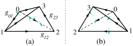
Figure 4: (Color online) Two branched simplices with opposite orientations. (a) A branched simplex with positive orientation and (b) a branched simplex with negative orientation.

In order to define a generic lattice theory on the space-time complex ${\cal M}^{D}$ using local Lagrangian term on each simplex, it is important to give the vertices of each simplex a local order. A nice local scheme to order the vertices is given by a branching structure.Costantino (2005); Chen et al. (2013, 2012) A branching structure is a choice of orientation of each link in the $d$-dimensional complex so that there is no oriented loop on any triangle (see Fig. 4).

The branching structure induces a local order of the vertices on each simplex. The first vertex of a simplex is the vertex with no incoming links, and the second vertex is the vertex with only one incoming link, etc . So the simplex in Fig. 4a has the following vertex ordering: $0,1,2,3$.

The branching structure also gives the simplex (and its sub-simplices) a canonical orientation. Fig. 4 illustrates two $3$-simplices with opposite canonical orientations compared with the 3-dimension space in which they are embedded. The blue arrows indicate the canonical orientations of the $2$-simplices. The black arrows indicate the canonical orientations of the $1$-simplices.

Given an Abelian group $(\mathbb{M},+)$, an $n$-cochain $f_{n}$ is an assignment of values in $\mathbb{M}$ to each $n$-simplex, for example a value $f_{n;i,j,\cdots,k}\in\mathbb{M}$ is assigned to $n$-simplex $(i,j,\cdots,k)$. So a cochain $f_{n}$ can be viewed as a bosonic field on the space-time lattice.

$\mathbb{M}$ can also be viewed a $\mathbb{Z}$-module (i.e. a vector space with integer coefficient) that also allows scaling by an integer:

$$x+y =z,\ \ \ \ x*y=z,\ \ \ \ mx=y,$$

$$x,y,z \in\mathbb{M},\ \ \ m\in\mathbb{Z}.$$ (248)

The direct sum of two modules $\mathbb{M}_{1}\oplus\mathbb{M}_{2}$ (as vector spaces) is equal to the direct product of the two modules (as sets):

$$\mathbb{M}_{1}\oplus\mathbb{M}_{2}\stackrel{{\scriptstyle\text{as set}}}{{=}}\mathbb{M}_{1}\times\mathbb{M}_{2}$$ (249)

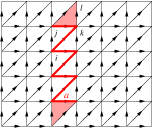
Figure 5: (Color online) A 1-cochain $a$ has a value $1$ on the red links: $a_{ik}=a_{jk}=1$ and a value $0$ on other links: $a_{ij}=a_{kl}=0$. $\hskip 1.0pt\mathrm{d}a$ is non-zero on the shaded triangles: $(\hskip 1.0pt\mathrm{d}a)_{jkl}=a_{jk}+a_{kl}-a_{jl}$. For such 1-cohain, we also have $a\smile a=0$. So when viewed as a $\mathbb{Z}_{2}$-valued cochain, $\beta_{2}a\neq a\smile a$ mod 2.

We like to remark that a simplex $(i,j,\cdots,k)$ can have two different orientations. We can use $(i,j,\cdots,k)$ and $(j,i,\cdots,k)=-(i,j,\cdots,k)$ to denote the same simplex with opposite orientations. The value $f_{n;i,j,\cdots,k}$ assigned to the simplex with opposite orientations should differ by a sign: $f_{n;i,j,\cdots,k}=-f_{n;j,i,\cdots,k}$. So to be more precise $f_{n}$ is a linear map $f_{n}:n\text{-simplex}\to\mathbb{M}$. We can denote the linear map as $\langle f_{n},n\text{-simplex}\rangle$, or

$$\langle f_{n},(i,j,\cdots,k)\rangle=f_{n;i,j,\cdots,k}\in\mathbb{M}.$$ (250)

More generally, a cochain $f_{n}$ is a linear map of $n$-chains:

$$f_{n}:n\text{-chains}\to\mathbb{M},$$ (251)

or (see Fig. 5)

$$\langle f_{n},n\text{-chain}\rangle\in\mathbb{M},$$ (252)

where a chain is a composition of simplices. For example, a 2-chain can be a 2-simplex: $(i,j,k)$, a sum of two 2-simplices: $(i,j,k)+(j,k,l)$, a more general composition of 2-simplices: $(i,j,k)-2(j,k,l)$, etc . The map $f_{n}$ is linear respect to such a composition. For example, if a chain is $m$ copies of a simplex, then its assigned value will be $m$ times that of the simplex. $m=-1$ correspond to an opposite orientation.

We will use $C^{n}({\cal M}^{D};\mathbb{M})$ to denote the set of all $n$-cochains on ${\cal M}^{D}$. $C^{n}({\cal M}^{D};\mathbb{M})$ can also be viewed as a set all $\mathbb{M}$-valued fields (or paths) on ${\cal M}^{D}$. Note that $C^{n}({\cal M}^{D};\mathbb{M})$ is an Abelian group under the $+$-operation.

The total space-time lattice ${\cal M}^{D}$ correspond to a $D$-chain. We will use the same ${\cal M}^{D}$ to denote it. Viewing $f_{D}$ as a linear map of $D$-chains, we can define an “integral” over ${\cal M}^{D}$:

$$\int_{{\cal M}^{D}}f_{D} \equiv\langle f_{D},{\cal M}^{D}\rangle$$ (253)

$$=\sum_{(i_{0},i_{1},\cdots,i_{D})}s_{i_{0}i_{1}\cdots i_{D}}(f_{D})_{i_{0},i_{1},\cdots,i_{D}}.$$

Here $s_{i_{0}i_{1}\cdots i_{D}}=\pm 1$, such that a $D$-simplex in the $D$-chain ${\cal M}^{D}$ is given by $s_{i_{0}i_{1}\cdots i_{D}}(i_{0},i_{1},\cdots,i_{D})$.

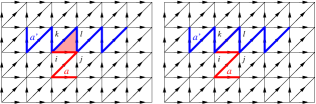
Figure 6: (Color online) A 1-cochain $a$ has a value $1$ on the red links, Another 1-cochain $a^{\prime}$ has a value $1$ on the blue links. On the left, $a\smile a^{\prime}$ is non-zero on the shade triangles: $(a\smile a^{\prime})_{ijl}=a_{ij}a^{\prime}_{jl}=1$. On the right, $a^{\prime}\smile a$ is zero on every triangle. Thus $a\smile a^{\prime}+a^{\prime}\smile a$ is not a coboundary.

We can define a derivative operator $\hskip 1.0pt\mathrm{d}$ acting on an $n$-cochain $f_{n}$, which give us an $n+1$-cochain (see Fig. 5):

$$\ \ \ \ \langle\hskip 1.0pt\mathrm{d}f_{n},(i_{0}i_{1}i_{2}\cdots i_{n+1})\rangle$$

$$=\sum_{m=0}^{n+1}(-)^{m}\langle f_{n},(i_{0}i_{1}i_{2}\cdots\hat{i}_{m}\cdots i_{n+1})\rangle$$ (254)

where $i_{0}i_{1}i_{2}\cdots\hat{i}_{m}\cdots i_{n+1}$ is the sequence $i_{0}i_{1}i_{2}\cdots i_{n+1}$ with $i_{m}$ removed, and $i_{0},i_{1},i_{2}\cdots i_{n+1}$ are the ordered vertices of the $(n+1)$-simplex $(i_{0}i_{1}i_{2}\cdots i_{n+1})$.

A cochain $f_{n}\in C^{n}({\cal M}^{D};\mathbb{M})$ is called a cocycle if $\hskip 1.0pt\mathrm{d}f_{n}=0$. The set of cocycles is denoted by $Z^{n}({\cal M}^{D};\mathbb{M})$. A cochain $f_{n}$ is called a coboundary if there exist a cochain $f_{n-1}$ such that $\hskip 1.0pt\mathrm{d}f_{n-1}=f_{n}$. The set of coboundaries is denoted by $B^{n}({\cal M}^{D};\mathbb{M})$. Both $Z^{n}({\cal M}^{D};\mathbb{M})$ and $B^{n}({\cal M}^{D};\mathbb{M})$ are Abelian groups as well. Since $\hskip 1.0pt\mathrm{d}^{2}=0$, a coboundary is always a cocycle: $B^{n}({\cal M}^{D};\mathbb{M})\subset Z^{n}({\cal M}^{D};\mathbb{M})$. We may view two cocycles differ by a coboundary as equivalent. The equivalence classes of cocycles, $[f_{n}]$, form the so called cohomology group denoted by

$$H^{n}({\cal M}^{D};\mathbb{M})=Z^{n}({\cal M}^{D};\mathbb{M})/B^{n}({\cal M}^{D};\mathbb{M}),$$ (255)

$H^{n}({\cal M}^{D};\mathbb{M})$, as a group quotient of $Z^{n}({\cal M}^{D};\mathbb{M})$ by $B^{n}({\cal M}^{D};\mathbb{M})$, is also an Abelian group.

When we study systems with time reversal symmetry, we need to consider cochains with local value. To define cochains with local value, we first note that a manifold ${\cal M}^{D}$ has a Stiefel-Whitney class ${\rm w}_{1}$ to describe its orientation structure. On each link $(ij)$ of ${\cal M}^{D}$, ${\rm w}_{1}$ has two values $({\rm w}_{1})_{ij}=0,1$. For a cochain $f$ with local values, we cannot directive compare their values on different simplexes, say $f_{ijk\cdots}$ and $f_{lmn\cdots}$. To compare $f_{ijk\cdots}$ and $f_{lmn\cdots}$, we need to use ${\rm w}_{1}$ to parallel transport the value $f_{lmn\cdots}$ with base point $l$ to the value with base point $i$: $f_{lmn\cdots}\to({\rm w}_{1})_{il}f_{lmn\cdots}$ then we can compare $f_{ijk\cdots}$ and $({\rm w}_{1})_{il}f_{lmn\cdots}$.

Such a interpretation of the value of a cochain will modify our definition of derivative operator

$$\ \ \ \ \langle\hskip 1.0pt\mathrm{d}_{{\rm w}_{1}}f_{n},(i_{0}i_{1}i_{2}\cdots i_{n+1})\rangle$$

$$=(-)^{({\rm w}_{1})_{01}}\langle f_{n},(i_{1}i_{2}\cdots i_{n+1})\rangle$$

$$\ \ \ \ +\sum_{m=1}^{n+1}(-)^{m}\langle f_{n},(i_{0}i_{1}i_{2}\cdots\hat{i}_{m}\cdots i_{n+1})\rangle$$ (256)

we note that on the right-hand-side of the above equation, all the terms have the base point $0$, except the first term which has a base point $1$.

In this paper, on orientable manifold $M^{D}$, we will choose ${\rm w}_{1}\overset{\scriptscriptstyle 2}{=}0$, and the cochains will all be the cochains with global values and the derivative operator is defined by eqn. (A). On the other hand, on unorientable manifold $M^{D}$, the cochains will all be the cochains with local values and the derivative operator is defined by eqn. (A). One can show that $\hskip 1.0pt\mathrm{d}$ and $\hskip 1.0pt\mathrm{d}_{{\rm w}_{1}}$ have the same local properties. We will drop the subscript ${\rm w}_{1}$ in $\hskip 1.0pt\mathrm{d}_{{\rm w}_{1}}$ and write $\hskip 1.0pt\mathrm{d}_{{\rm w}_{1}}$ as $\hskip 1.0pt\mathrm{d}$.

For the $\mathbb{Z}_{N}$-valued cocycle $x_{n}$, $\hskip 1.0pt\mathrm{d}x_{n}\overset{\scriptscriptstyle N}{=}0$. Thus

$$\beta_{N}x_{n}\equiv\frac{1}{N}\hskip 1.0pt\mathrm{d}x_{n}$$ (257)

is a $\mathbb{Z}$-valued cocycle. Here $\beta_{N}$ is Bockstrin homomorphism.

We notice the above definition for cochains still makes sense if we have a non-Abelian group $(G,\cdot)$ instead of an Abelian group $(\mathbb{M},+)$, however the differential $\hskip 1.0pt\mathrm{d}$ defined by eqn. (A) will not satisfy $\hskip 1.0pt\mathrm{d}\circ\hskip 1.0pt\mathrm{d}=1$, except for the first two $\hskip 1.0pt\mathrm{d}$’s. That is, one may still make sense of 0-cocycle and 1-cocycle, but no more further naively by formula eqn. (A). For us, we only use non-Abelian 1-cocycle in this article. Thus it is ok. Non-Abelian cohomology is then thoroughly studied in mathematics motivating concepts such as gerbes to enter.

From two cochains $f_{m}$ and $h_{n}$, we can construct a third cochain $p_{m+n}$ via the cup product (see Fig. 6):

$$p_{m+n} =f_{m}\smile h_{n},$$

$$\langle p_{m+n},(0\to{m+n})\rangle =\langle f_{m},(0\to m)\rangle\times$$

$$\ \ \ \ \langle h_{n},(m\to{m+n})\rangle,$$ (258)

where $i\to j$ is the consecutive sequence from $i$ to $j$:

$$i\to j\equiv i,i+1,\cdots,j-1,j.$$ (259)

Note that the above definition applies to cochains with global. If $h_{n}$ has a local value, we then have

$$p_{m+n} =f_{m}\smile h_{n},$$

$$\langle p_{m+n},(0\to{m+n})\rangle =(-)^{({\rm w}_{1})_{0m}}\langle f_{m},(0\to m)\rangle\times$$

$$\ \ \ \ \langle h_{n},(m\to{m+n})\rangle,$$ (260)

The cup product has the following property

$$\hskip 1.0pt\mathrm{d}(f_{m}\smile h_{n}) =(\hskip 1.0pt\mathrm{d}h_{n})\smile f_{m}+(-)^{n}h_{n}\smile(\hskip 1.0pt\mathrm{d}f_{m})$$ (261)

for cochains with global or local values. We note that the above is a local relation. Locally, we can always choose a gauge to make ${\rm w}_{1}\overset{\scriptscriptstyle 2}{=}0$. Thus, the local relations are valid for cochains with both global and local values.

We see that $f_{m}\smile h_{n}$ is a cocycle if both $f_{m}$ and $h_{n}$ are cocycles. If both $f_{m}$ and $h_{n}$ are cocycles, then $f_{m}\smile h_{n}$ is a coboundary if one of $f_{m}$ and $h_{n}$ is a coboundary. So the cup product is also an operation on cohomology groups $\underset{{\scriptscriptstyle}}{\smile}:H^{m}(M^{D};\mathbb{M})\times H^{n}(M^{D};\mathbb{M})\to H^{m+n}(M^{D};\mathbb{M})$. The cup product of two cocycles has the following property (see Fig. 6)

$$f_{m}\smile h_{n} =(-)^{mn}h_{n}\smile f_{m}+\text{coboundary}$$ (262)

We can also define higher cup product $f_{m}\underset{{\scriptscriptstyle k}}{\smile}h_{n}$ which gives rise to a $(m+n-k)$-cochain Steenrod (1947):

$$\ \ \ \ \langle f_{m}\underset{{\scriptscriptstyle k}}{\smile}h_{n},(0,1,\cdots,m+n-k)\rangle$$

$$=\hskip-10.00002pt\sum_{0\leq i_{0}<\cdots<i_{k}\leq n+m-k}\hskip-30.00005pt(-)^{p}\langle f_{m},(0\to i_{0},i_{1}\to i_{2},\cdots)\rangle\times$$

$$\ \ \ \ \ \ \ \ \ \ \ \ \ \ \ \ \ \ \ \ \langle h_{n},(i_{0}\to i_{1},i_{2}\to i_{3},\cdots)\rangle,$$ (263)

and $f_{m}\underset{{\scriptscriptstyle k}}{\smile}h_{n}=0$ for $k<0$ or for $k>m\text{ or }n$. Here $i\to j$ is the sequence $i,i+1,\cdots,j-1,j$, and $p$ is the number of permutations to bring the sequence

$$0\to i_{0},i_{1}\to i_{2},\cdots;i_{0}+1\to i_{1}-1,i_{2}+1\to i_{3}-1,\cdots$$ (264)

to the sequence

$$0\to m+n-k.$$ (265)

For example

$$\langle f_{m}\underset{{\scriptscriptstyle 1}}{\smile}h_{n},(0\to m+n-1)\rangle=\sum_{i=0}^{m-1}(-)^{(m-i)(n+1)}\times$$

$$\langle f_{m},(0\to i,i+n\to m+n-1)\rangle\langle h_{n},(i\to i+n)\rangle.$$ (266)

We can see that $\underset{{\scriptscriptstyle 0}}{\smile}=\smile$. Unlike cup product at $k=0$, the higher cup product of two cocycles may not be a cocycle. For cochains $f_{m},h_{n}$, we have

$$\hskip 1.0pt\mathrm{d}(f_{m}\underset{{\scriptscriptstyle k}}{\smile}h_{n})=\hskip 1.0pt\mathrm{d}f_{m}\underset{{\scriptscriptstyle k}}{\smile}h_{n}+(-)^{m}f_{m}\underset{{\scriptscriptstyle k}}{\smile}\hskip 1.0pt\mathrm{d}h_{n}+$$ (267)

$$\ \ \ (-)^{m+n-k}f_{m}\underset{{\scriptscriptstyle k-1}}{\smile}h_{n}+(-)^{mn+m+n}h_{n}\underset{{\scriptscriptstyle k-1}}{\smile}f_{m}$$

If $h_{n}$ has a local value, we then have

$$\ \ \ \ \langle f_{m}\underset{{\scriptscriptstyle k}}{\smile}h_{n},(0,1,\cdots,m+n-k)\rangle$$

$$=\hskip-10.00002pt\sum_{0\leq i_{0}<\cdots<i_{k}\leq n+m-k}\hskip-30.00005pt(-)^{p}(-)^{({\rm w}_{1})_{0i_{0}}}\langle f_{m},(0\to i_{0},i_{1}\to i_{2},\cdots)\rangle\times$$

$$\ \ \ \ \ \ \ \ \ \ \ \ \ \ \ \ \ \ \ \ \langle h_{n},(i_{0}\to i_{1},i_{2}\to i_{3},\cdots)\rangle,$$ (268)

Let $f_{m}$ and $h_{n}$ be cocycles and $c_{l}$ be a chain, from eqn. (267) we can obtain

$$\hskip 1.0pt\mathrm{d}(f_{m}\underset{{\scriptscriptstyle k}}{\smile}h_{n})=(-)^{m+n-k}f_{m}\underset{{\scriptscriptstyle k-1}}{\smile}h_{n}$$

$$\ \ \ \ \ \ \ \ \ \ \ \ \ \ \ \ \ +(-)^{mn+m+n}h_{n}\underset{{\scriptscriptstyle k-1}}{\smile}f_{m},$$

$$\hskip 1.0pt\mathrm{d}(f_{m}\underset{{\scriptscriptstyle k}}{\smile}f_{m})=[(-)^{k}+(-)^{m}]f_{m}\underset{{\scriptscriptstyle k-1}}{\smile}f_{m},$$

$$\hskip 1.0pt\mathrm{d}(c_{l}\underset{{\scriptscriptstyle k-1}}{\smile}c_{l}+c_{l}\underset{{\scriptscriptstyle k}}{\smile}\hskip 1.0pt\mathrm{d}c_{l})=\hskip 1.0pt\mathrm{d}c_{l}\underset{{\scriptscriptstyle k}}{\smile}\hskip 1.0pt\mathrm{d}c_{l}$$

$$\ \ \ -[(-)^{k}-(-)^{l}](c_{l}\underset{{\scriptscriptstyle k-2}}{\smile}c_{l}+c_{l}\underset{{\scriptscriptstyle k-1}}{\smile}\hskip 1.0pt\mathrm{d}c_{l}).$$ (269)

From eqn. (A), we see that, for $\mathbb{Z}_{2}$-valued cocycles $z_{n}$,

$$\text{Sq}^{n-k}(z_{n})\equiv z_{n}\underset{{\scriptscriptstyle k}}{\smile}z_{n}$$ (270)

is always a cocycle. Here Sq is called the Steenrod square. More generally $h_{n}\underset{{\scriptscriptstyle k}}{\smile}h_{n}$ is a cocycle if $n+k=$ odd and $h_{n}$ is a cocycle. Usually, the Steenrod square is defined only for $\mathbb{Z}_{2}$-valued cocycles or cohomology classes. Here, we like to define a generalized Steenrod square for $\mathbb{M}$-valued cochains $c_{n}$:

$$\mathbb{Sq}^{n-k}c_{n}\equiv c_{n}\underset{{\scriptscriptstyle k}}{\smile}c_{n}+c_{n}\underset{{\scriptscriptstyle k+1}}{\smile}\hskip 1.0pt\mathrm{d}c_{n}.$$ (271)

From eqn. (A), we see that

$$\hskip 1.0pt\mathrm{d}\mathbb{Sq}^{k}c_{n} =\hskip 1.0pt\mathrm{d}(c_{n}\underset{{\scriptscriptstyle n-k}}{\smile}c_{n}+c_{n}\underset{{\scriptscriptstyle n-k+1}}{\smile}\hskip 1.0pt\mathrm{d}c_{n})$$ (272)

$$=\mathbb{Sq}^{k}\hskip 1.0pt\mathrm{d}c_{n}+(-)^{n}\begin{cases}0,&k=\text{odd}\\ 2\mathbb{Sq}^{k+1}c_{n}&k=\text{even}\\ \end{cases}.$$

In particular, when $c_{n}$ is a $\mathbb{Z}_{2}$-valued cochain, we have

$$\hskip 1.0pt\mathrm{d}\mathbb{Sq}^{k}c_{n}\overset{\scriptscriptstyle 2}{=}\mathbb{Sq}^{k}\hskip 1.0pt\mathrm{d}c_{n}.$$ (273)

Next, let us consider the action of $\mathbb{Sq}^{k}$ on the sum of two $\mathbb{M}$-valued cochains $c_{n}$ and $c_{n}^{\prime}$:

$$\mathbb{Sq}^{k}(c_{n}+c_{n}^{\prime})=\mathbb{Sq}^{k}c_{n}+\mathbb{Sq}^{k}c_{n}^{\prime}+$$

$$\ \ \ c_{n}\underset{{\scriptscriptstyle n-k}}{\smile}c_{n}^{\prime}+c_{n}^{\prime}\underset{{\scriptscriptstyle n-k}}{\smile}c_{n}+c_{n}\underset{{\scriptscriptstyle n-k+1}}{\smile}\hskip 1.0pt\mathrm{d}c_{n}^{\prime}+c_{n}^{\prime}\underset{{\scriptscriptstyle n-k+1}}{\smile}\hskip 1.0pt\mathrm{d}c_{n}$$

$$=\mathbb{Sq}^{k}c_{n}+\mathbb{Sq}^{k}c_{n}^{\prime}+[1+(-)^{k}]c_{n}\underset{{\scriptscriptstyle n-k}}{\smile}c_{n}^{\prime}$$

$$\ \ \ -(-)^{n-k}[-(-)^{n-k}c_{n}^{\prime}\underset{{\scriptscriptstyle n-k}}{\smile}c_{n}+(-)^{n}c_{n}\underset{{\scriptscriptstyle n-k}}{\smile}c_{n}^{\prime}]$$

$$\ \ \ +c_{n}\underset{{\scriptscriptstyle n-k+1}}{\smile}\hskip 1.0pt\mathrm{d}c_{n}^{\prime}+c_{n}^{\prime}\underset{{\scriptscriptstyle n-k+1}}{\smile}\hskip 1.0pt\mathrm{d}c_{n}$$

$$=\mathbb{Sq}^{k}c_{n}+\mathbb{Sq}^{k}c_{n}^{\prime}+[1+(-)^{k}]c_{n}\underset{{\scriptscriptstyle n-k}}{\smile}c_{n}^{\prime}$$

$$+(-)^{n-k}[\hskip 1.0pt\mathrm{d}c_{n}^{\prime}\underset{{\scriptscriptstyle n-k+1}}{\smile}c_{n}+(-)^{n}c_{n}^{\prime}\underset{{\scriptscriptstyle n-k+1}}{\smile}\hskip 1.0pt\mathrm{d}c_{n}]$$

$$-(-)^{n-k}\hskip 1.0pt\mathrm{d}(c_{n}^{\prime}\underset{{\scriptscriptstyle n-k+1}}{\smile}c_{n})+c_{n}\underset{{\scriptscriptstyle n-k+1}}{\smile}\hskip 1.0pt\mathrm{d}c_{n}^{\prime}+c_{n}^{\prime}\underset{{\scriptscriptstyle n-k+1}}{\smile}\hskip 1.0pt\mathrm{d}c_{n}$$

$$=\mathbb{Sq}^{k}c_{n}+\mathbb{Sq}^{k}c_{n}^{\prime}+[1+(-)^{k}]c_{n}\underset{{\scriptscriptstyle n-k}}{\smile}c_{n}^{\prime}$$

$$\ \ \ +[1+(-)^{k}]c_{n}^{\prime}\underset{{\scriptscriptstyle n-k+1}}{\smile}\hskip 1.0pt\mathrm{d}c_{n}-(-)^{n-k}\hskip 1.0pt\mathrm{d}(c_{n}^{\prime}\underset{{\scriptscriptstyle n-k+1}}{\smile}c_{n})$$

$$\ \ \ -[(-)^{n-k+1}\hskip 1.0pt\mathrm{d}c_{n}^{\prime}\underset{{\scriptscriptstyle n-k+1}}{\smile}c_{n}-c_{n}\underset{{\scriptscriptstyle n-k+1}}{\smile}\hskip 1.0pt\mathrm{d}c_{n}^{\prime}]$$

$$=\mathbb{Sq}^{k}c_{n}+\mathbb{Sq}^{k}c_{n}^{\prime}+[1+(-)^{k}]c_{n}\underset{{\scriptscriptstyle n-k}}{\smile}c_{n}^{\prime}$$

$$\ \ \ +[1+(-)^{k}]c_{n}^{\prime}\underset{{\scriptscriptstyle n-k+1}}{\smile}\hskip 1.0pt\mathrm{d}c_{n}-(-)^{n-k}\hskip 1.0pt\mathrm{d}(c_{n}^{\prime}\underset{{\scriptscriptstyle n-k+1}}{\smile}c_{n})$$

$$\ \ \ -\hskip 1.0pt\mathrm{d}(\hskip 1.0pt\mathrm{d}c_{n}^{\prime}\underset{{\scriptscriptstyle n-k+2}}{\smile}c_{n})+\hskip 1.0pt\mathrm{d}c_{n}^{\prime}\underset{{\scriptscriptstyle n-k+2}}{\smile}\hskip 1.0pt\mathrm{d}c_{n}$$

$$=\mathbb{Sq}^{k}c_{n}+\mathbb{Sq}^{k}c_{n}^{\prime}+\hskip 1.0pt\mathrm{d}c_{n}^{\prime}\underset{{\scriptscriptstyle n-k+2}}{\smile}\hskip 1.0pt\mathrm{d}c_{n}$$

$$\ \ \ +[1+(-)^{k}][c_{n}\underset{{\scriptscriptstyle n-k}}{\smile}c_{n}^{\prime}+c_{n}^{\prime}\underset{{\scriptscriptstyle n-k+1}}{\smile}\hskip 1.0pt\mathrm{d}c_{n}]$$

$$\ \ \ -(-)^{n-k}\hskip 1.0pt\mathrm{d}(c_{n}^{\prime}\underset{{\scriptscriptstyle n-k+1}}{\smile}c_{n})-\hskip 1.0pt\mathrm{d}(\hskip 1.0pt\mathrm{d}c_{n}^{\prime}\underset{{\scriptscriptstyle n-k+2}}{\smile}c_{n}).$$ (274)

We see that, if one of the $c_{n}$ and $c_{n}^{\prime}$ is a cocycle,

$$\mathbb{Sq}^{k}(c_{n}+c_{n}^{\prime})\overset{\scriptscriptstyle 2,\hskip 1.0pt\mathrm{d}}{=}\mathbb{Sq}^{k}c_{n}+\mathbb{Sq}^{k}c_{n}^{\prime}.$$ (275)

We also see that

$$\ \ \ \ \mathbb{Sq}^{k}(c_{n}+\hskip 1.0pt\mathrm{d}f_{n-1})$$ (276)

$$=\mathbb{Sq}^{k}c_{n}+\mathbb{Sq}^{k}\hskip 1.0pt\mathrm{d}f_{n-1}+[1+(-)^{k}]\hskip 1.0pt\mathrm{d}f_{n-1}\underset{{\scriptscriptstyle n-k}}{\smile}c_{n}$$

$$\ \ \ -(-)^{n-k}\hskip 1.0pt\mathrm{d}(c_{n}\underset{{\scriptscriptstyle n-k+1}}{\smile}\hskip 1.0pt\mathrm{d}f_{n-1})-\hskip 1.0pt\mathrm{d}(\hskip 1.0pt\mathrm{d}c_{n}\underset{{\scriptscriptstyle n-k+2}}{\smile}\hskip 1.0pt\mathrm{d}f_{n-1})$$

$$=\mathbb{Sq}^{k}c_{n}+[1+(-)^{k}][\hskip 1.0pt\mathrm{d}f_{n-1}\underset{{\scriptscriptstyle n-k}}{\smile}c_{n}+(-)^{n}\mathbb{Sq}^{k+1}f_{n-1}]$$

$$+\hskip 1.0pt\mathrm{d}[\mathbb{Sq}^{k}f_{n-1}-(-)^{n-k}c_{n}\hskip-5.0pt\underset{{\scriptscriptstyle n-k+1}}{\smile}\hskip-5.0pt\hskip 1.0pt\mathrm{d}f_{n-1}-\hskip 1.0pt\mathrm{d}c_{n}\hskip-5.0pt\underset{{\scriptscriptstyle n-k+2}}{\smile}\hskip-5.0pt\hskip 1.0pt\mathrm{d}f_{n-1}]$$

$$=\mathbb{Sq}^{k}c_{n}+[1+(-)^{k}][c_{n}\underset{{\scriptscriptstyle n-k}}{\smile}\hskip 1.0pt\mathrm{d}f_{n-1}+(-)^{n}\mathbb{Sq}^{k+1}f_{n-1}]$$

$$+\hskip 1.0pt\mathrm{d}[\mathbb{Sq}^{k}f_{n-1}-(-)^{n-k}\hskip 1.0pt\mathrm{d}f_{n-1}\underset{{\scriptscriptstyle n-k+1}}{\smile}c_{n}].$$

Using eqn. (A), we can also obtain the following result if $\hskip 1.0pt\mathrm{d}c_{n}=$ even

$$\ \ \ \ \mathbb{Sq}^{k}(c_{n}+2c_{n}^{\prime})$$

$$\overset{\scriptscriptstyle 4}{=}\mathbb{Sq}^{k}c_{n}+2\hskip 1.0pt\mathrm{d}(c_{n}\underset{{\scriptscriptstyle n-k+1}}{\smile}c_{n}^{\prime})+2\hskip 1.0pt\mathrm{d}c_{n}\underset{{\scriptscriptstyle n-k+1}}{\smile}c_{n}^{\prime}$$

$$\overset{\scriptscriptstyle 4}{=}\mathbb{Sq}^{k}c_{n}+2\hskip 1.0pt\mathrm{d}(c_{n}\underset{{\scriptscriptstyle n-k+1}}{\smile}c_{n}^{\prime})$$ (277)

As another application, we note that, for a $\mathbb{M}$-valued cochain $m_{d}$ and using eqn. (267),

$$\mathbb{Sq}^{1}(m_{d})=m_{d}\underset{{\scriptscriptstyle d-1}}{\smile}m_{d}+m_{d}\underset{{\scriptscriptstyle d}}{\smile}\hskip 1.0pt\mathrm{d}m_{d}$$

$$=\frac{1}{2}(-)^{d}[\hskip 1.0pt\mathrm{d}(m_{d}\underset{{\scriptscriptstyle d}}{\smile}m_{d})-\hskip 1.0pt\mathrm{d}m_{d}\underset{{\scriptscriptstyle d}}{\smile}m_{d}]+\frac{1}{2}m_{d}\underset{{\scriptscriptstyle d}}{\smile}\hskip 1.0pt\mathrm{d}m_{d}$$

$$=(-)^{d}\beta_{2}(m_{d}\underset{{\scriptscriptstyle d}}{\smile}m_{d})-(-)^{d}\beta_{2}m_{d}\underset{{\scriptscriptstyle d}}{\smile}m_{d}+m_{d}\underset{{\scriptscriptstyle d}}{\smile}\beta_{2}m_{d}$$

$$=(-)^{d}\beta_{2}\mathbb{Sq}^{0}m_{d}-2(-)^{d}\beta_{2}m_{d}\underset{{\scriptscriptstyle d+1}}{\smile}\beta_{2}m_{d}$$

$$=(-)^{d}\beta_{2}\mathbb{Sq}^{0}m_{d}-2(-)^{d}\mathbb{Sq}^{0}\beta_{2}m_{d}$$ (278)

This way, we obtain a relation between Steenrod square and Bockstein homomorphism, when $m_{d}$ is a $\mathbb{Z}_{2}$-valued cochain

$$\mathbb{Sq}^{1}(m_{d})\overset{\scriptscriptstyle 2}{=}\beta_{2}m_{d},$$ (279)

where we have used $\mathbb{Sq}^{0}m_{d}=m_{d}$ for $\mathbb{Z}_{2}$-valued cochain.

Appendix B Almost cocycle and almost coboundary

A ${\mathbb{R}/\mathbb{Z}}$-valued cocycle $c$ satisfies

$$\hskip 1.0pt\mathrm{d}c\overset{\scriptscriptstyle 1}{=}0.$$ (280)

A ${\mathbb{R}/\mathbb{Z}}$-valued almost-cocycle $\tilde{c}$ satisfies

$$\hskip 1.0pt\mathrm{d}\tilde{c}\overset{\scriptscriptstyle 1}{\approx}0.$$ (281)

Physically, it is impossible to constrain an ${\mathbb{R}/\mathbb{Z}}$-value to exactly zero. So almost-cocycle is more relevant for our model construction. In this paper, when we refer ${\mathbb{R}/\mathbb{Z}}$-valued cocycle, we really mean ${\mathbb{R}/\mathbb{Z}}$-valued almost-cocycle.

Similarly, a ${\mathbb{R}/\mathbb{Z}}$-valued almost-coboundary is given by

$$\hskip 1.0pt\mathrm{d}c+\epsilon,$$ (282)

where $\epsilon$ is an almost-zero cochain.

The cohomology class $H^{*}_{\text{a}}(M;{\mathbb{R}/\mathbb{Z}})$ for ${\mathbb{R}/\mathbb{Z}}$-valued almost-cocycles is different from the cohomology class $H^{*}(M;{\mathbb{R}/\mathbb{Z}})$ for ${\mathbb{R}/\mathbb{Z}}$-valued cocycles. For example, let us consider $H^{1}_{\text{a}}(S^{2};{\mathbb{R}/\mathbb{Z}})$. We parametrize $S^{2}$ by the polar angle $\theta$, and the azimuthal angle $\phi$. The 1-cochain

$$\tilde{a}^{{\mathbb{R}/\mathbb{Z}}}=\frac{1-\cos(\theta)}{4\pi}\hskip 1.0pt\mathrm{d}\phi$$ (283)

is not a cocycle since $\hskip 1.0pt\mathrm{d}\tilde{a}^{{\mathbb{R}/\mathbb{Z}}}\neq 0$ mod 1. But it is an 1-almost-cocycle since

$$\hskip 1.0pt\mathrm{d}\tilde{a}^{{\mathbb{R}/\mathbb{Z}}}\approx c_{1},$$ (284)

and $c_{1}$ is a $\mathbb{Z}$-valued. $\tilde{a}^{{\mathbb{R}/\mathbb{Z}}}$ is not an 1-almost-coboundary, since $c_{1}$ generates $H^{2}(S^{2};\mathbb{Z})$. In fact, $\tilde{a}^{{\mathbb{R}/\mathbb{Z}}}$ is the generator of $H^{1}_{\text{a}}(S^{2};{\mathbb{R}/\mathbb{Z}})$ and we have

$$H^{1}_{\text{a}}(S^{2};{\mathbb{R}/\mathbb{Z}})\cong H^{2}(S^{2};\mathbb{Z})=\mathbb{Z}.$$ (285)

In contrast $H^{1}(S^{2};{\mathbb{R}/\mathbb{Z}})=0$.

In general, for an almost-cocycle $\tilde{c}$,

$$\lfloor\hskip 1.0pt\mathrm{d}\tilde{c}\rfloor=C$$ (286)

is a $\mathbb{Z}$-valued cocycle. The non-trivialness of $\tilde{c}$ is given by the non-trivialness of $C$. Thus we have

$$H^{n}_{\text{a}}(M;{\mathbb{R}/\mathbb{Z}})\cong H^{n+1}(M;\mathbb{Z}).$$ (287)

In this paper, we will drop the subscript and write $H^{n}_{\text{a}}(M;{\mathbb{R}/\mathbb{Z}})$ as $H^{n}(M;{\mathbb{R}/\mathbb{Z}})$.

Appendix C Some additional discussion of fermion decoration

C.1 Another form of exactly soluble local fermionic models

We can also write the path integral eqn. (VI) as one on $M^{d+1}$. To do so, we introduce a new $\mathbb{Z}_{2}$-valued $(d-1)$-cochain field $b_{d-1}$ that satisfy

$$\hskip 1.0pt\mathrm{d}b_{d-1}\overset{\scriptscriptstyle 2}{=}f_{d}$$ (288)

to write the integrant of $\int_{N^{d+2}}$ as a total derivative (using eqn. (273))

$$\ \ \ \ \hskip 1.0pt\mathrm{d}[\mathbb{Sq}^{2}b_{d-1}+b_{d-1}({\rm w}_{2}+{\rm w}_{1}^{2})]$$

$$\overset{\scriptscriptstyle 2}{=}\text{Sq}^{2}n_{d}+n_{d}({\rm w}_{2}+{\rm w}_{1}^{2}).$$ (289)

This way, we can change the path integral eqn. (VI) to one on $M^{d+1}$ only:

$$Z(M^{d+1},A^{G_{b}}) =\hskip-47.00003pt\sum_{g\in C^{0}(M^{d+1};G_{b});f_{d}\overset{\scriptscriptstyle 2}{=}n_{d}(a^{G_{b}})}\hskip-47.00003pt\hskip 1.0pt\mathrm{e}^{\hskip 1.0pt\mathrm{i}\hskip 1.0pt2\pi\int_{M^{d+1}}\nu_{d+1}(a^{G_{b}})+\frac{1}{2}\mathbb{Sq}^{2}b_{d-1}+\frac{1}{2}b_{d-1}e_{2}},$$ (290)

where $b_{d-1}$ is a function of $f_{d}$ as determined from eqn. (288). The summation $\sum_{g\in C^{0}(M^{d+1};G_{b});f_{d}\overset{\scriptscriptstyle 2}{=}n_{d}(a^{G_{b}})}$ (i.e. the path integral) is over a $G_{b}$-valued 0-cochain field $g$ and $\mathbb{Z}_{2}$-valued $d$-cochain field $f_{d}$. But $f_{d}$ subject to a constrain $f_{d}\overset{\scriptscriptstyle 2}{=}n_{d}(a^{G_{b}})=n_{d}(g_{i}A^{G_{b}}_{ij}g_{j}^{-1})$, which can be imposed as an energy penalty. The term $\frac{1}{2}\mathbb{Sq}^{2}b_{d-1}$ makes the current $f_{d}$ a fermion current (i.e. makes the field $f_{d}$ to describe a fermion).

In order for eqn. (290) to be well defined, the action amplitude $\hskip 1.0pt\mathrm{e}^{\hskip 1.0pt\mathrm{i}\hskip 1.0pt2\pi\int_{M^{d+1}}\nu_{d+1}(a^{G_{b}})+\frac{1}{2}[\mathbb{Sq}^{2}b_{d-1}+b_{d-1}e_{2}(a^{G_{b}})]}$ should be a function of $f_{d}$ and does not depend on which solution $b_{d-1}$ of $\hskip 1.0pt\mathrm{d}b_{d-1}\overset{\scriptscriptstyle 2}{=}f_{d}$ that we choose. Different solutions can differ by a cocycle $\bar{b}_{d-1}$. Using eqn. (A), we find that

$$\mathbb{Sq}^{2}(b_{d-1}+\bar{b}_{d-1})+(b_{d-1}+\bar{b}_{d-1})e_{2}-\mathbb{Sq}^{2}b_{d-1}-b_{d-1}e_{2}$$

$$\overset{\scriptscriptstyle 2,\hskip 1.0pt\mathrm{d}}{=}\mathbb{Sq}^{2}(\bar{b}_{d-1})+\bar{b}_{d-1}e_{2}(a^{G_{b}})$$

$$\overset{\scriptscriptstyle 2,\hskip 1.0pt\mathrm{d}}{=}\bar{b}_{d-1}[{\rm w}_{2}+{\rm w}_{1}^{2}+e_{2}(A^{G_{b}})].$$ (291)

Thus the path integral is well defined only on $M^{d+1}$ with a symmetry twist $A$ such that ${\rm w}_{2}+{\rm w}_{1}^{2}+e_{2}(A^{G_{b}})\overset{\scriptscriptstyle 2,\hskip 1.0pt\mathrm{d}}{=}0$. This implies that $f_{d}$ describes a fermion. This also implies that the fermion is described by a representation of $G_{f}=Z_{2}\leftthreetimes_{e_{2}}G_{b}$ (see LABEL:ZLW).

C.2 Exactly soluble local bosonic models with emergent fermions

If we treat the field $b_{d-1}$ in eqn. (290) as an independent dynamical field (instead of as a function of $f_{d}$), then we will get a very different theory:

$$Z(M^{d+1},A^{G_{b}})=\hskip-55.00008pt\sum_{g\in C^{0}(M^{d+1};G_{b});\hskip 1.0pt\mathrm{d}b_{d-1}\overset{\scriptscriptstyle 2}{=}n_{d}(a^{G_{b}})}\hskip-55.00008pt\hskip 1.0pt\mathrm{e}^{\hskip 1.0pt\mathrm{i}\hskip 1.0pt\pi\int_{M^{d+1}}2\nu_{d+1}(a^{G_{b}})+\mathbb{Sq}^{2}b_{d-1}+b_{d-1}e_{2}(a^{G_{b}})},$$ (292)

The new path integral eqn. (292) sums over the 0-cochains $g_{i}$ and $(d-1)$-cochains $b_{d-1}$ satisfying $\hskip 1.0pt\mathrm{d}b_{d-1}=n_{d}(a^{G_{b}})$. Such a model is actually a local bosonic model. The local bosonic model has emergent fermions whose current is given by $f_{d}=\hskip 1.0pt\mathrm{d}b_{d-1}-n_{d}(a^{G_{b}})$.

The above local bosonic model has a $G_{b}$ symmetry. Thus the model describes symmetry $G_{b}$ enriched topological order with emergent fermions. If we break the $G_{b}$ symmetry, the model describes a $Z_{2}$-topological order with emergent fermion. Such a $Z_{2}$-topological is described by a $Z_{2}$ gauge theory where the $Z_{2}$ charge is fermionic. In the presence of $G_{b}$ symmetry, the emergent fermions carry fractionalized symmetry quantum number. Since the partition function of the local bosonic model vanishes when ${\rm w}_{2}+{\rm w}_{1}^{2}+e_{2}(A^{G_{b}})\neq 0$, we conclude that the emergent fermions carry representations of $G_{f}=Z_{2}\leftthreetimes_{e_{2}}G_{b}$. The partition function of the local bosonic model vanishes when ${\rm w}_{2}+{\rm w}_{1}^{2}+e_{2}(A^{G_{b}})\neq 0$. We may view eqn. (VI) as a fermionic model with $G_{f}$ symmetry, and the bosonic model (292) as the $Z_{2}^{f}$ gauged fermionic model. If we gauge all the symmetry $G_{f}$ in the fermionic model (VI), we will obtain a higher gauge theory as described in LABEL:ZLW:

$$Z(M^{d+1})=\hskip-90.00014pt\sum_{\ \ \ \ \ \ \ \ \ \ \ \ \ \ \ \ \ \ \ \ a^{G_{b}}\in C^{1}(M^{d+1};G_{b});\hskip 1.0pt\mathrm{d}b_{d-1}=n_{d}(a^{G_{b}})}\hskip-90.00014pt\hskip 1.0pt\mathrm{e}^{\hskip 1.0pt\mathrm{i}\hskip 1.0pt\pi\int_{M^{d+1}}2\nu_{d+1}(a^{G_{b}})+\mathbb{Sq}^{2}b_{d-1}+b_{d-1}e_{2}(a^{G_{b}})}.$$ (293)

Despite their similarity, the two local bosonic models (292) and (293) are very different. In eqn. (292), the dynamical fields are $g,b_{d-1}$ (with $a^{G_{b}}_{ij}=g_{i}A^{G_{b}}_{ij}g_{j}^{-1}$), where $g$ is a $G_{b}$-valued 0-cochain living on vertices. In contrast, in eqn. (292), the dynamical fields are $a^{G_{b}},b_{d-1}$ where $a^{G_{b}}$ is a $G_{b}$-valued 1-cochain living on links.

C.3 Another connection to higher gauge theory

There is another connection to higher gauge theory. After gauging all the $G_{f}$ symmetry in the fermionic model eqn. (VI), we obtain a local bosonic model eqn. (293). Such a local bosonic model is a higher gauge theory with emergent fermion. Such a higher gauge theory is characterized by a higher group and its cocycle. Thus the data that characterizes a fermionic SPT phase is closely related to a higher group and its cocycle.

In fact the local bosonic theory eqn. (293) is characterized by a higher group ${\cal G}_{n_{d}}(G_{b},1;Z_{2}^{f},d-1)$ and its higher-group cocycle $\omega_{d+1}$. The field content $a^{G_{b}},b_{d-1}$ and their conditions

$$(\delta a^{G_{b}})_{ijk} \equiv a^{G_{b}}_{ij}a^{G_{b}}_{jk}a^{G_{b}}_{ki}=1$$

$$\hskip 1.0pt\mathrm{d}b_{d-1} \overset{\scriptscriptstyle 2}{=}n_{d}(a^{G_{b}}),$$ (294)

determine the higher group ${\cal G}_{n_{d}}(G_{b},1;Z_{2}^{f},d-1)$, which can be viewed as a space with homotopy groups $\pi_{1}=G_{b}$, $\pi_{d-1}=Z_{2}^{f}$, and other $\pi_{n}=0$.

The local bosonic model eqn. (293) and eqn. (292) are exactly soluble if the Lagrangian is given by a higher-group cocycle satisfying $\hskip 1.0pt\mathrm{d}\omega_{d+1}\overset{\scriptscriptstyle 1}{=}0$ (i.e. $\omega_{d+1}\in Z^{d+1}[{\cal G}_{n_{d}}(G_{b},1;Z_{2}^{f},d-1);\mathbb{R}/\mathbb{Z}]$):

$$\ \ \ \ \omega_{d+1}(a^{G_{b}},b_{d-1})$$

$$=\nu_{d+1}(a^{G_{b}})+\frac{1}{2}[\mathbb{Sq}^{2}b_{d-1}+n_{d}(a^{G_{b}})e_{2}(a^{G_{b}})],$$ (295)

(See LABEL:ZLW and Appendix L for an introduction on higher groups and higher-group cocycles.)

Appendix D Operations on modules

The tensor-product operation $\otimes_{R}$ and the torsion-product operation $\text{Tor}_{1}^{R}$ act on $R$-modules $\mathbb{M},\mathbb{M}^{\prime},\mathbb{M}^{\prime\prime}$. Here $R$ is a ring and a $R$-module is like a vector space over $R$ (i.e. we can “multiply” a “vector” in $\mathbb{M}$ by an element of $R$, and two “vectors” in $\mathbb{M}$ can add.) The tensor-product operation $\otimes_{R}$ has the following properties:

$$\mathbb{M}\otimes_{\mathbb{Z}}\mathbb{M}^{\prime}\simeq\mathbb{M}^{\prime}\otimes_{\mathbb{Z}}\mathbb{M},$$

$$(\mathbb{M}^{\prime}\oplus\mathbb{M}^{\prime\prime})\otimes_{R}\mathbb{M}=(\mathbb{M}^{\prime}\otimes_{R}\mathbb{M})\oplus(\mathbb{M}^{\prime\prime}\otimes_{R}\mathbb{M}),$$

$$\mathbb{M}\otimes_{R}(\mathbb{M}^{\prime}\oplus\mathbb{M}^{\prime\prime})=(\mathbb{M}\otimes_{R}\mathbb{M}^{\prime})\oplus(\mathbb{M}\otimes_{R}\mathbb{M}^{\prime\prime});$$

$$\mathbb{Z}\otimes_{\mathbb{Z}}\mathbb{M}\simeq\mathbb{M}\otimes_{\mathbb{Z}}\mathbb{Z}=\mathbb{M},$$

$$\mathbb{Z}_{n}\otimes_{\mathbb{Z}}\mathbb{M}\simeq\mathbb{M}\otimes_{\mathbb{Z}}\mathbb{Z}_{n}=\mathbb{M}/n\mathbb{M},$$

$$\mathbb{Z}_{n}\otimes_{\mathbb{Z}}{\mathbb{R}/\mathbb{Z}}\simeq{\mathbb{R}/\mathbb{Z}}\otimes_{\mathbb{Z}}\mathbb{Z}_{n}=0,$$

$$\mathbb{Z}_{m}\otimes_{\mathbb{Z}}\mathbb{Z}_{n}=\mathbb{Z}_{\langle m,n\rangle},$$

$$\mathbb{R}\otimes_{\mathbb{Z}}{\mathbb{R}/\mathbb{Z}}=0,$$

$$\mathbb{R}\otimes_{\mathbb{Z}}\mathbb{R}=\mathbb{R}.$$ (296)

The torsion-product operation $\text{Tor}_{1}^{R}$ has the following properties:

$$\text{Tor}^{1}_{R}(\mathbb{M},\mathbb{M}^{\prime})\simeq\text{Tor}^{1}_{R}(\mathbb{M}^{\prime},\mathbb{M}),$$

$$\text{Tor}^{1}_{R}(\mathbb{M}^{\prime}\oplus\mathbb{M}^{\prime\prime},\mathbb{M})=\text{Tor}^{1}_{R}(\mathbb{M}^{\prime},\mathbb{M})\oplus\text{Tor}^{1}_{R}(\mathbb{M}^{\prime\prime},\mathbb{M}),$$

$$\text{Tor}^{1}_{R}(\mathbb{M},\mathbb{M}^{\prime}\oplus\mathbb{M}^{\prime\prime})=\text{Tor}^{1}_{R}(\mathbb{M},\mathbb{M}^{\prime})\oplus\text{Tor}^{1}_{R}(\mathbb{M},\mathbb{M}^{\prime\prime})$$

$$\text{Tor}^{1}_{\mathbb{Z}}(\mathbb{Z},\mathbb{M})=\text{Tor}^{1}_{\mathbb{Z}}(\mathbb{M},\mathbb{Z})=0,$$

$$\text{Tor}^{1}_{\mathbb{Z}}(\mathbb{Z}_{n},\mathbb{M})=\{m\in\mathbb{M}|nm=0\},$$

$$\text{Tor}^{1}_{\mathbb{Z}}(\mathbb{Z}_{n},{\mathbb{R}/\mathbb{Z}})=\mathbb{Z}_{n},$$

$$\text{Tor}^{1}_{\mathbb{Z}}(\mathbb{Z}_{m},\mathbb{Z}_{n})=\mathbb{Z}_{\langle m,n\rangle},$$

$$\text{Tor}^{1}_{\mathbb{Z}}(\mathbb{R}/\mathbb{Z},\mathbb{R}/\mathbb{Z})=0.$$ (297)

These expressions allow us to compute the tensor-product $\otimes_{R}$ and the torsion-product $\text{Tor}^{1}_{R}$. We will use abbreviated Tor to denote $\text{Tor}^{1}_{\mathbb{Z}}$.

In addition to $\otimes_{\mathbb{Z}}$ and Tor, we also have Ext and Hom operations on modules. Ext operation is given by

$$\text{Ext}^{1}_{R}(\mathbb{M}^{\prime}\oplus\mathbb{M}^{\prime\prime},\mathbb{M})=\text{Ext}^{1}_{R}(\mathbb{M}^{\prime},\mathbb{M})\oplus\text{Ext}^{1}_{R}(\mathbb{M}^{\prime\prime},\mathbb{M}),$$

$$\text{Ext}^{1}_{R}(\mathbb{M},\mathbb{M}^{\prime}\oplus\mathbb{M}^{\prime\prime})=\text{Ext}^{1}_{R}(\mathbb{M},\mathbb{M}^{\prime})\oplus\text{Ext}^{1}_{R}(\mathbb{M},\mathbb{M}^{\prime\prime})$$

$$\text{Ext}^{1}_{\mathbb{Z}}(\mathbb{Z},\mathbb{M})=0,$$

$$\text{Ext}^{1}_{\mathbb{Z}}(\mathbb{Z}_{n},\mathbb{M})=\mathbb{M}/n\mathbb{M},$$

$$\text{Ext}^{1}_{\mathbb{Z}}(\mathbb{Z}_{n},\mathbb{Z})=\mathbb{Z}_{n},$$

$$\text{Ext}^{1}_{\mathbb{Z}}(\mathbb{Z}_{n},{\mathbb{R}/\mathbb{Z}})=0,$$

$$\text{Ext}^{1}_{\mathbb{Z}}(\mathbb{Z}_{m},\mathbb{Z}_{n})=\mathbb{Z}_{\langle m,n\rangle},.$$ (298)

The Hom operation on modules is given by

$$\text{Hom}_{R}(\mathbb{M}^{\prime}\oplus\mathbb{M}^{\prime\prime},\mathbb{M})=\text{Hom}_{R}(\mathbb{M}^{\prime},\mathbb{M})\oplus\text{Hom}_{R}(\mathbb{M}^{\prime\prime},\mathbb{M}),$$

$$\text{Hom}_{R}(\mathbb{M},\mathbb{M}^{\prime}\oplus\mathbb{M}^{\prime\prime})=\text{Hom}_{R}(\mathbb{M},\mathbb{M}^{\prime})\oplus\text{Hom}_{R}(\mathbb{M},\mathbb{M}^{\prime\prime}),$$

$$\text{Hom}_{\mathbb{Z}}(\mathbb{Z},\mathbb{M})=\mathbb{M},$$

$$\text{Hom}_{\mathbb{Z}}(\mathbb{Z}_{n},\mathbb{M})=\{m\in\mathbb{M}|nm=0\},$$

$$\text{Hom}_{\mathbb{Z}}(\mathbb{Z}_{n},\mathbb{Z})=0,$$

$$\text{Hom}_{\mathbb{Z}}(\mathbb{Z}_{n},{\mathbb{R}/\mathbb{Z}})=\mathbb{Z}_{n},$$

$$\text{Hom}_{\mathbb{Z}}(\mathbb{Z}_{m},\mathbb{Z}_{n})=\mathbb{Z}_{\langle m,n\rangle}.$$ (299)

We will use abbreviated Ext and Hom to denote $\text{Ext}^{1}_{\mathbb{Z}}$ and $\text{Hom}_{\mathbb{Z}}$.

Appendix E Künneth formula and universal coefficient theorem

The Künneth formula is a very helpful formula that allows us to calculate the cohomology of chain complex $X\times X^{\prime}$ in terms of the cohomology of chain complex $X$ and chain complex $X^{\prime}$. The Künneth formula is expressed in terms of the tensor-product operation $\otimes_{R}$ and the torsion-product operation $\text{Tor}_{1}^{R}$ described in the last section (see LABEL:Spa66 page 247):

$$0 \to\bigoplus_{k=0}^{d}H^{k}(X,\mathbb{M})\otimes_{R}H^{d-k}(X^{\prime},\mathbb{M}^{\prime})$$

$$\to H^{d}(X\times X^{\prime},\mathbb{M}\otimes_{R}\mathbb{M}^{\prime})$$

$$\to\bigoplus_{k=0}^{d+1}\text{Tor}_{R}^{1}(H^{k}(X,\mathbb{M}),H^{d-k+1}(X^{\prime},\mathbb{M}^{\prime}))\to 0,$$ (300)

where the exact sequence is split. Here $R$ is a principle ideal domain and $\mathbb{M},\mathbb{M}^{\prime}$ are $R$-modules such that $\text{Tor}_{R}^{1}(\mathbb{M},\mathbb{M}^{\prime})=0$. We also require either
(1) $H_{d}(X,\mathbb{Z})$ and $H_{d}(X^{\prime},\mathbb{Z})$ are finitely generated, or
(2) $\mathbb{M}^{\prime}$ and $H_{d}(X^{\prime},\mathbb{Z})$ are finitely generated.
(For example, $\mathbb{M}^{\prime}=\mathbb{Z}\oplus\cdots\oplus\mathbb{Z}\oplus\mathbb{Z}_{n}\oplus\cdots\oplus\mathbb{Z}_{m}$ is finitely generated, with $R=\mathbb{Z}$.)

For more details on principal ideal domain and $R$-module, see the corresponding Wiki articles. Note that ring $\mathbb{Z}$ and $\mathbb{R}$ are principal ideal domains. Also, $\mathbb{R}$ and $\mathbb{R}/\mathbb{Z}$ are not finitely generate $R$-modules if $R=\mathbb{Z}$.

The Künneth formula works for topological cohomology where $X$ and $X^{\prime}$ are treated as topological spaces.

As the first application of Künneth formula, we like to use it to calculate $H^{*}(X^{\prime},\mathbb{M})$ from $H^{*}(X^{\prime},\mathbb{Z})$, by choosing $R=\mathbb{M}^{\prime}=\mathbb{Z}$. In this case, the condition $\text{Tor}_{R}^{1}(\mathbb{M},\mathbb{M}^{\prime})=\text{Tor}_{\mathbb{Z}}^{1}(\mathbb{M},\mathbb{Z})=0$ is always satisfied. $\mathbb{M}$ can be $\mathbb{R}/\mathbb{Z}$, $\mathbb{Z}$, $\mathbb{Z}_{n}$ etc . So we have

$$0 \to\bigoplus_{k=0}^{d}H^{k}(X,\mathbb{M})\otimes_{\mathbb{Z}}H^{d-k}(X^{\prime},\mathbb{Z})$$

$$\to H^{d}(X\times X^{\prime},\mathbb{M})$$

$$\to\bigoplus_{k=0}^{d}\text{Tor}(H^{k}(X,{\mathbb{M}}),H^{d-k+1}(X^{\prime},\mathbb{Z}))\to 0$$ (301)

Again, the exact sequence is split.

We can further choose $X$ to be the space of one point in eqn. (E), and use

$$H^{d}(X,\mathbb{M}))=\begin{cases}\mathbb{M},&\text{ if }d=0,\\ 0,&\text{ if }d>0,\end{cases}$$ (302)

to reduce eqn. (E) to

$$H^{d}(X,\mathbb{M}) \simeq\mathbb{M}\otimes_{\mathbb{Z}}H^{d}(X,\mathbb{Z})\oplus\text{Tor}(\mathbb{M},H^{d+1}(X,\mathbb{Z})).$$ (303)

where $X^{\prime}$ is renamed as $X$. The above is a form of the universal coefficient theorem which can be used to calculate $H^{*}(X,\mathbb{M})$ from $H^{*}(X,\mathbb{Z})$ and the module $\mathbb{M}$.

Using the universal coefficient theorem, we can rewrite eqn. (E) as

$$H^{d}(X\times X^{\prime},\mathbb{M})\simeq\bigoplus_{k=0}^{d}H^{k}[X,H^{d-k}(X^{\prime},\mathbb{M})].$$ (304)

The above is valid for topological cohomology.

Appendix F Lyndon-Hochschild-Serre spectral sequence

The Lyndon-Hochschild-Serre spectral sequence (see LABEL:L4871 page 280,291, and LABEL:HS5310) allows us to understand the structure of of the cohomology of a fiber bundle $F\to X\to B$, $H^{*}(X;\mathbb{M})$, from $H^{*}(F;\mathbb{M})$ and $H^{*}(B;\mathbb{M})$. In general, $H^{d}(X;\mathbb{M})$, when viewed as an Abelian group, contains a chain of subgroups

$$\{0\}=H_{d+1}\subset H_{d}\subset\cdots\subset H_{0}=H^{d}(X;\mathbb{M})$$ (305)

such that $H_{l}/H_{l+1}$ is a subgroup of a factor group of $H^{l}[B,H^{d-l}(F;\mathbb{M})_{B}]$, i.e. $H^{l}[B,H^{d-l}(F;\mathbb{M})_{B}]$ contains a subgroup $\Gamma^{k}$, such that

$$H_{l}/H_{l+1} \subset H^{l}[B,H^{d-l}(F;\mathbb{M})_{B}]/\Gamma^{l},$$

$$l =0,\cdots,d.$$ (306)

Note that $\pi_{1}(B)$ may have a non-trivial action on $\mathbb{M}$ and $\pi_{1}(B)$ may have a non-trivial action on $H^{d-l}(F;\mathbb{M})$ as determined by the structure $F\to X\to B$. We add the subscript $B$ to $H^{d-l}(F;\mathbb{M})$ to indicate this action. We also have

$$H_{0}/H_{1} \subset H^{0}[B,H^{d}(F;\mathbb{M})_{B}],$$

$$H_{d}/H_{d+1} =H_{d}=H^{d}(B;\mathbb{M})/\Gamma^{d}.$$ (307)

In other words, all the elements in $H^{d}(X;\mathbb{M})$ can be one-to-one labeled by $(x_{0},x_{1},\cdots,x_{d})$ with

$$x_{l}\in H_{l}/H_{l+1}\subset H^{l}[B,H^{d-l}(F;\mathbb{M})_{B}]/\Gamma^{l}.$$ (308)

Let $x_{l,\alpha}$, $\alpha=1,2,\cdots$, be the generators of $H^{l}/H^{l+1}$. Then we say $x_{i,\alpha}$ for all $l,\alpha$ are the generators of $H^{d}(X;\mathbb{M})$. We also call $H_{l}/H_{l+1}$, $l=0,\cdots,d$, the generating sub-factor groups of $H^{d}(X;\mathbb{M})$.

The above result implies that we can use $(k_{0},k_{1},\cdots,k_{d})$ with $k_{l}\in H^{l}[B,H^{d-l}(F;\mathbb{M})_{B}]$ to label all the elements in $H^{d}(X;\mathbb{M})$. However, such a labeling scheme may not be one-to-one, and it may happen that only some of $(k_{0},k_{1},\cdots,k_{d})$ correspond to the elements in $H^{d}(X;\mathbb{M})$. But, on the other hand, for every element in $H^{d}(X;\mathbb{M})$, we can find a $(k_{0},k_{1},\cdots,k_{d})$ that corresponds to it. Such a relation can be described by an injective map

$$H^{d}(F\leftthreetimes B;\mathbb{M})\rightarrowtail\bigoplus_{l=0}^{d}H^{l}[B,H^{d-l}(F;\mathbb{M})_{B}]$$ (309)

For the special case $X=B\times F$, $(k_{0},k_{1},\cdots,k_{d})$ will give us an one-to-one labeling of the elements in $H^{d}(B\times F;\mathbb{M})$. In fact

$$H^{d}(B \times F;\mathbb{M})=\bigoplus_{l=0}^{d}H^{l}[B,H^{d-l}(F;\mathbb{M})].$$ (310)

Appendix G The ring of $H^{*}({\cal B}SO_{\infty};\mathbb{Z})$

The ring $H^{*}({\cal B}SO_{n};\mathbb{Z}_{2})$ has a simple structure:

$$H^{*}({\cal B}SO_{n};\mathbb{Z}_{2})=\mathbb{Z}_{2}[{\rm w}_{2},{\rm w}_{3},\cdots,{\rm w}_{n}].$$ (311)

According to LABEL:B8283, the ring $H^{*}({\cal B}SO_{n};\mathbb{Z})$ is given by

$$H^{*}({\cal B}SO_{\infty};\mathbb{Z})=\mathbb{Z}[\{p_{i}\},\{\beta_{2}({\rm w}_{2i_{1}}{\rm w}_{2i_{2}}\cdots)\},X_{n}]/\sim,$$ (312)

where $\mathbb{Z}[\{p_{i}\},\{\beta_{2}({\rm w}_{2i_{1}}{\rm w}_{2i_{2}}\cdots)\},X_{n}]$ is a polynomial ring generated by $p_{i}$ and $\beta_{2}({\rm w}_{2i_{1}}{\rm w}_{2i_{2}}\cdots)$, $0<i\leq\lfloor\frac{n-1}{2}\rfloor$, $0<i_{1}<i_{2}<\cdots\leq\lfloor\frac{n-1}{2}\rfloor$, with integer coefficients. Here $p_{i}\in H^{4i}({\cal B}SO_{\infty};\mathbb{Z})$ is the Pontryagin class of dimension $4i$ and ${\rm w}_{i}\in H^{i}({\cal B}SO_{\infty};\mathbb{Z}_{2})$ is the Stiefel-Whitney class of dimension $i$. Since $\text{Tor}H^{d}({\cal B}G,{\mathbb{R}/\mathbb{Z}})=\text{Tor}H^{d+1}({\cal B}G;\mathbb{Z})$ (see, for example, LABEL:W1313), the natural map $H^{d}({\cal B}G;\mathbb{Z}_{2})\to\text{Tor}H^{d}({\cal B}G,{\mathbb{R}/\mathbb{Z}})$ induces the Bockstein homomorphism $H^{d}({\cal B}G;\mathbb{Z}_{2})\to H^{d+1}({\cal B}G;\mathbb{Z})$: $\beta_{2}:H^{i}({\cal B}SO_{\infty};\mathbb{Z}_{2})\to H^{i+1}({\cal B}SO_{\infty};\mathbb{Z})$. Note that $f\in H^{i}({\cal B}SO_{\infty};\mathbb{Z}_{2})$ satisfies $\hskip 1.0pt\mathrm{d}f\overset{\scriptscriptstyle 2}{=}0$. Thus $\frac{1}{2}\hskip 1.0pt\mathrm{d}f\overset{\scriptscriptstyle 1}{=}0$, or $\frac{1}{2}\hskip 1.0pt\mathrm{d}f$ is an integral cocycle. This allows us to write the Bockstein homomorphism as

$$\beta_{2}f=\frac{1}{2}\hskip 1.0pt\mathrm{d}f\in H^{i+1}({\cal B}SO_{\infty};\mathbb{Z}).$$ (313)

To obtain the ring $H^{*}({\cal B}SO_{\infty};\mathbb{Z})$ from a polynomial ring generated by $p_{i}$ and $\beta_{2}({\rm w}_{2i_{1}}{\rm w}_{2i_{2}}\cdots)$, we need to quotient out certain equivalence relations $\sim$. The equivalence relations $\sim$ contain

$$2\beta_{2}({\rm w}_{2i_{1}}{\rm w}_{2i_{2}}\cdots) =0,\ \ \ \ p_{n}\overset{\scriptscriptstyle 2}{=}{\rm w}_{2n}^{2},\ \ \ \ X_{n}=\beta_{2}{\rm w}_{2k}\text{ if }n=2k+1,\ \ \ \ X_{n}^{2}=p_{k}\text{ if }n=2k,$$ (314)

$$\beta_{2}w(I)\beta_{2}w(J) =\sum_{k\in I}\beta_{2}{\rm w}_{2k}\ \beta_{2}{\rm w}[(I-\{k\})\cup J-(I-\{k\})\cap J]\ p[(I-\{k\})\cap J],$$

where $I=\{i_{1},i_{2},\cdots\}$, ${\rm w}(I)={\rm w}_{2i_{1}}{\rm w}_{2i_{2}}\cdots$. and $p(I)=p_{i_{1}}p_{i_{2}}\cdots$. Many last kind of the equivalence relations are trivial identities. The first non-trivial equivalence relations appears at dimension 14:

$$\beta_{2}({\rm w}_{4}{\rm w}_{2})\beta_{2}{\rm w}_{6}=\beta_{2}{\rm w}_{4}\beta_{2}({\rm w}_{6}{\rm w}_{2})+\beta_{2}{\rm w}_{2}\beta_{2}({\rm w}_{6}{\rm w}_{4}),$$

$$\beta_{2}({\rm w}_{4}{\rm w}_{2})\beta_{2}({\rm w}_{4}{\rm w}_{2})=p_{1}\beta_{2}{\rm w}_{4}\beta_{2}{\rm w}_{4}+p_{2}\beta_{2}{\rm w}_{2}\beta_{2}{\rm w}_{2}.$$ (315)

We see that there are no effective equivalence relations of the last kind for dimensions less than 14. So for low dimensions,

$$H^{0}({\cal B}SO_{\infty};\mathbb{Z}) =\mathbb{Z},$$

$$H^{1}({\cal B}SO_{\infty};\mathbb{Z}) =0,$$

$$H^{2}({\cal B}SO_{\infty};\mathbb{Z}) =0,$$

$$H^{3}({\cal B}SO_{\infty};\mathbb{Z}) =\mathbb{Z}_{2}=\{\beta_{2}{\rm w}_{2}\},$$

$$H^{4}({\cal B}SO_{\infty};\mathbb{Z}) =\mathbb{Z}=\{p_{1}\},$$

$$H^{5}({\cal B}SO_{\infty};\mathbb{Z}) =\mathbb{Z}_{2}=\{\beta_{2}{\rm w}_{4}\},$$ (316)

$$H^{6}({\cal B}SO_{\infty};\mathbb{Z}) =\mathbb{Z}_{2}=\{\beta_{2}{\rm w}_{2}\beta_{2}{\rm w}_{2}\},$$

$$H^{7}({\cal B}SO_{\infty};\mathbb{Z}) =\mathbb{Z}_{2}^{\oplus 3}=\{\beta_{2}{\rm w}_{6},\beta_{2}({\rm w}_{2}{\rm w}_{4}),p_{1}\beta_{2}{\rm w}_{2}\},$$

$$H^{8}({\cal B}SO_{\infty};\mathbb{Z}) =\mathbb{Z}^{\oplus 2}\oplus\mathbb{Z}_{2}=\{p_{1}^{2},p_{2},\beta_{2}{\rm w}_{2}\beta_{2}{\rm w}_{4}\}.$$

In the above, we also list the basis (or generators) of cohomology classes. Using eqn. (287), the above allows us to obtain

$$H_{\text{a}}^{0}({\cal B}SO_{\infty};{\mathbb{R}/\mathbb{Z}}) =0,$$

$$H_{\text{a}}^{1}({\cal B}SO_{\infty};{\mathbb{R}/\mathbb{Z}}) =0,$$

$$H_{\text{a}}^{2}({\cal B}SO_{\infty};{\mathbb{R}/\mathbb{Z}}) =\mathbb{Z}_{2}=\{\frac{1}{2}{\rm w}_{2}\},$$

$$H_{\text{a}}^{3}({\cal B}SO_{\infty};{\mathbb{R}/\mathbb{Z}}) =\mathbb{Z}=\{\omega_{3}\},$$

$$H_{\text{a}}^{4}({\cal B}SO_{\infty};{\mathbb{R}/\mathbb{Z}}) =\mathbb{Z}_{2}=\{\frac{1}{2}{\rm w}_{4}\},$$ (317)

$$H_{\text{a}}^{5}({\cal B}SO_{\infty};{\mathbb{R}/\mathbb{Z}}) =\mathbb{Z}_{2}=\{\frac{1}{2}{\rm w}_{2}{\rm w}_{3})\},$$

$$H_{\text{a}}^{6}({\cal B}SO_{\infty};{\mathbb{R}/\mathbb{Z}}) =\mathbb{Z}_{2}^{\oplus 3}=\{\frac{1}{2}{\rm w}_{6},\frac{1}{2}{\rm w}_{2}{\rm w}_{4},\frac{1}{2}p_{1}{\rm w}_{2}\},$$

$$H_{\text{a}}^{7}({\cal B}SO_{\infty};{\mathbb{R}/\mathbb{Z}}) =\mathbb{Z}^{\oplus 2}\oplus\mathbb{Z}_{2}=\{\omega_{3}p_{1},\omega_{7},\frac{1}{2}{\rm w}_{3}{\rm w}_{4}\}.$$

where $\omega_{4n-1}$ is a $\mathbb{R}/\mathbb{Z}$-valued almost-cocycle on ${\cal B}SO_{\infty}$ (the gravitational Chern-Simons term)

$$\hskip 1.0pt\mathrm{d}\omega_{4n-1}=p_{n}.$$ (318)

The above basis give rise to the basis in eqn. (G) through the natural map $\beta$: $H^{d}({\cal B}G,{\mathbb{R}/\mathbb{Z}})\to H^{d+1}({\cal B}G,\mathbb{Z})$.

Appendix H The ring of $H^{*}({\cal B}O_{\infty};\mathbb{Z})$

The ring $H^{*}({\cal B}O_{n};\mathbb{Z}_{2})$ is given by

$$H^{*}({\cal B}O_{n};\mathbb{Z}_{2})=\mathbb{Z}_{2}[{\rm w}_{1},{\rm w}_{2},\cdots,{\rm w}_{n}].$$ (319)

and the ring $H^{*}({\cal B}O_{\infty};\mathbb{Z})$ is given byBrown (1982)

$$H^{*}({\cal B}O_{\infty};\mathbb{Z})=\mathbb{Z}[\{p_{i}\},\{\beta_{2}({\rm w}_{1}^{\epsilon}{\rm w}_{2i_{1}}{\rm w}_{2i_{2}}\cdots)\}]/\sim,$$ (320)

where $\mathbb{Z}[\{p_{i}\},\{\beta_{2}({\rm w}_{1}^{\epsilon}{\rm w}_{2i_{1}}{\rm w}_{2i_{2}}\cdots)\}]$ is a polynomial ring with integer coefficients, generated by $p_{i}$ and $\beta_{2}({\rm w}_{1}^{\epsilon}{\rm w}_{2i_{1}}{\rm w}_{2i_{2}}\cdots)$, $\epsilon=0,1$, $0<i\leq\lfloor\frac{n}{2}\rfloor$, and $0<i_{1}<i_{2}<\cdots\leq\lfloor\frac{n}{2}\rfloor$. Here $p_{i}\in H^{4i}({\cal B}O_{\infty};\mathbb{Z})$ is the Pontryagin class of dimension $4i$ and ${\rm w}_{i}\in H^{i}({\cal B}O_{\infty};\mathbb{Z}_{2})$ is the Stiefel-Whitney class of dimension $i$.

To obtain the ring $H^{*}({\cal B}O_{\infty};\mathbb{Z})$ from a polynomial ring generated by $p_{i}$ and $\beta_{2}({\rm w}_{1}^{\epsilon}{\rm w}_{2i_{1}}{\rm w}_{2i_{2}}\cdots)$, we need to quotient out certain equivalence relations $\sim$. The equivalence relations $\sim$ contain

$$2\beta_{2}({\rm w}_{2i_{1}}{\rm w}_{2i_{2}}\cdots) =0,\ \ \ \beta_{2}({\rm w}_{1}{\rm w}_{n})=0,\ \ \ p_{n}\overset{\scriptscriptstyle 2}{=}{\rm w}_{2n}^{2},\ \ \ (\beta_{2}{\rm w}_{n})^{2}\big{|}_{n=\text{even}}=p_{n/2}\beta_{2}{\rm w}_{1},$$ (321)

$$\beta_{2}{\rm w}(I)\beta_{2}{\rm w}(J) =\sum_{k\in I}\beta_{2}{\rm w}_{2k}\ \beta_{2}{\rm w}[(I-\{k\})\cup J-(I-\{k\})\cap J]\ p[(I-\{k\})\cap J],$$

where $I=\{\frac{\epsilon}{2},i_{1},i_{2},\cdots\}$, ${\rm w}(I)={\rm w}_{1}^{\epsilon}{\rm w}_{2i_{1}}{\rm w}_{2i_{2}}\cdots$, and $p(I)={\rm w}_{1}^{\epsilon}p_{i_{1}}p_{i_{2}}\cdots$. Many last kind of the equivalence relations are trivial identities. The non-trivial equivalence relations for dimension 9 and less are given by:

$$[\beta_{2}({\rm w}_{1}{\rm w}_{2})]^{2} =(\beta_{2}{\rm w}_{2})^{2}\beta_{2}{\rm w}_{1}+(\beta_{2}{\rm w}_{1})^{2}p_{1},$$

$$\beta_{2}({\rm w}_{1}{\rm w}_{2})\beta_{2}{\rm w}_{4} =\beta_{2}{\rm w}_{2}\beta_{2}({\rm w}_{1}{\rm w}_{4})+\beta_{2}{\rm w}_{1}\beta_{2}({\rm w}_{2}{\rm w}_{4})$$ (322)

So for low dimensions,

$$H^{0}({\cal B}O_{\infty};\mathbb{Z}) =\mathbb{Z},$$

$$H^{1}({\cal B}O_{\infty};\mathbb{Z}) =0,$$

$$H^{2}({\cal B}O_{\infty};\mathbb{Z}) =\mathbb{Z}_{2}=\{\beta_{2}{\rm w}_{1}\},$$

$$H^{3}({\cal B}O_{\infty};\mathbb{Z}) =\mathbb{Z}_{2}=\{\beta_{2}{\rm w}_{2}\},$$

$$H^{4}({\cal B}O_{\infty};\mathbb{Z}) =\mathbb{Z}_{2}\oplus\mathbb{Z}=\{(\beta_{2}{\rm w}_{1})^{2},p_{1}\},$$

$$H^{5}({\cal B}O_{\infty};\mathbb{Z}) =\mathbb{Z}_{2}^{\oplus 2}=\{\beta_{2}{\rm w}_{4},\beta_{2}{\rm w}_{1}\beta_{2}{\rm w}_{2}\},$$ (323)

$$H^{6}({\cal B}O_{\infty};\mathbb{Z}) =\mathbb{Z}_{2}^{\oplus 3}=\{(\beta_{2}{\rm w}_{2})^{2},(\beta_{2}{\rm w}_{1})^{3},p_{1}\beta_{2}{\rm w}_{1}\},$$

$$H^{7}({\cal B}O_{\infty};\mathbb{Z}) =\mathbb{Z}_{2}^{\oplus 5}=\{\beta_{2}{\rm w}_{6},\beta_{2}({\rm w}_{2}{\rm w}_{4}),$$

$$p_{1}\beta_{2}{\rm w}_{2},(\beta_{2}{\rm w}_{1})^{2}\beta_{2}{\rm w}_{2},\beta_{2}{\rm w}_{1}\beta_{2}{\rm w}_{4}\},$$

$$H^{8}({\cal B}O_{\infty};\mathbb{Z}) =\mathbb{Z}_{2}^{\oplus 5}\oplus\mathbb{Z}^{\oplus 2}=\{\beta_{2}({\rm w}_{1}{\rm w}_{2}{\rm w}_{4}),(\beta_{2}{\rm w}_{1})^{4},$$

$$\beta_{2}{\rm w}_{2}\beta_{2}{\rm w}_{4},\beta_{2}{\rm w}_{1}(\beta_{2}{\rm w}_{2})^{2},p_{1}(\beta_{2}{\rm w}_{1})^{2},p_{1}^{2},p_{2}\}.$$

In the above, we also list the basis (or generators) of cohomology classes. Due to the relation eqn. (287), the above allows us to obtain

$$H_{\text{a}}^{0}({\cal B}O_{\infty};{\mathbb{R}/\mathbb{Z}}) =\mathbb{R}/\mathbb{Z},$$

$$H_{\text{a}}^{1}({\cal B}O_{\infty};{\mathbb{R}/\mathbb{Z}}) =\mathbb{Z}_{2}=\{\frac{1}{2}{\rm w}_{1}\},$$

$$H_{\text{a}}^{2}({\cal B}O_{\infty};{\mathbb{R}/\mathbb{Z}}) =\mathbb{Z}_{2}=\{\frac{1}{2}{\rm w}_{2}\},$$

$$H_{\text{a}}^{3}({\cal B}O_{\infty};{\mathbb{R}/\mathbb{Z}}) =\mathbb{Z}_{2}\oplus\mathbb{Z}=\{\frac{1}{2}{\rm w}_{1}\beta_{2}{\rm w}_{1},\omega_{3}\},$$

$$H_{\text{a}}^{4}({\cal B}O_{\infty};{\mathbb{R}/\mathbb{Z}}) =\mathbb{Z}_{2}^{\oplus 2}=\{\frac{1}{2}{\rm w}_{4},\frac{1}{2}{\rm w}_{1}\beta_{2}{\rm w}_{2}\},$$ (324)

$$H_{\text{a}}^{5}({\cal B}O_{\infty};{\mathbb{R}/\mathbb{Z}}) =\mathbb{Z}_{2}^{\oplus 3}=\{\frac{1}{2}{\rm w}_{2}\beta_{2}{\rm w}_{2},\frac{1}{2}{\rm w}_{1}(\beta_{2}{\rm w}_{1})^{2},\frac{1}{2}{\rm w}_{1}p_{1}\},$$

$$H_{\text{a}}^{6}({\cal B}O_{\infty};{\mathbb{R}/\mathbb{Z}}) =\mathbb{Z}_{2}^{\oplus 5}=\{\frac{1}{2}{\rm w}_{6},\frac{1}{2}{\rm w}_{2}{\rm w}_{4},\frac{1}{2}{\rm w}_{2}p_{1},$$

$$\frac{1}{2}{\rm w}_{2}(\beta_{2}{\rm w}_{1})^{2},\frac{1}{2}{\rm w}_{1}\beta_{2}{\rm w}_{4}\},$$

$$H_{\text{a}}^{7}({\cal B}O_{\infty};{\mathbb{R}/\mathbb{Z}}) =\mathbb{Z}_{2}^{\oplus 5}\oplus\mathbb{Z}^{\oplus 2}=\{\frac{1}{2}{\rm w}_{1}{\rm w}_{2}{\rm w}_{4},\frac{1}{2}{\rm w}_{1}(\beta_{2}{\rm w}_{1})^{3},$$

$$\frac{1}{2}{\rm w}_{2}\beta_{2}{\rm w}_{4}, \frac{1}{2}{\rm w}_{1}(\beta_{2}{\rm w}_{2})^{2},\frac{1}{2}{\rm w}_{1}p_{1}\beta_{2}{\rm w}_{1},\omega_{3}p_{1},\omega_{7}\}.$$

Appendix I Relations between cocycles and Stiefel-Whitney classes on a closed manifold

The cocycles and the Stiefel-Whitney classes on a closed manifold satisfy many relations. In this section, we will show how to generate those relations.

I.1 Introduction to Stiefel-Whitney classes

The Stiefel-Whitney classes ${\rm w}_{i}\in H^{i}(M^{D};\mathbb{Z}_{2})$ is defined for an $O_{n}$ vector bundle on a $d$-dimensional space with $n\to\infty$. If the $O_{\infty}$ vector bundle on $d$-dimensional space, $M^{D}$, happen to be the tangent bundle of $M^{D}$ direct summed with a trivial $\infty$-dimensional vector bundle, then the corresponding Stiefel-Whitney classes are referred as the Stiefel-Whitney classes of the manifold $M^{D}$.

The Stiefel-Whitney classes of manifold behave well under the connected sum of manifolds. Let

$${\rm w}(M)=1+{\rm w}_{1}(M)+{\rm w}_{2}(M)+\cdots$$ (325)

be the total Stiefel-Whitney class of a manifold $M$. If we know ${\rm w}(M)$ and ${\rm w}(N)$, then we can obtain ${\rm w}(M\#N)$:

$${\rm w}(M\#N)\overset{\scriptscriptstyle 2,\hskip 1.0pt\mathrm{d}}{=}{\rm w}(M)+{\rm w}(N)-1.$$ (326)

Under the product of manifolds, we have

$${\rm w}(M\times N)\overset{\scriptscriptstyle 2,\hskip 1.0pt\mathrm{d}}{=}{\rm w}(M){\rm w}(N).$$ (327)

The Stiefel-Whitney numbers are non-oriented cobordism invariant. All the Stiefel-Whitney numbers of a smooth compact manifold vanish iff the manifold is the boundary of some smooth compact manifold. Here the manifold can be non-orientable.

The Stiefel-Whitney numbers and Pontryagin numbers are oriented cobordism invariant. All the Stiefel-Whitney numbers and Pontryagin numbers of a smooth compact orientable manifold vanish iff the manifold is the boundary of some smooth compact orientable manifold.

I.2 Relations between Stiefel-Whitney classes of the tangent bundle

For generic $O_{\infty}$ vector bundle, the Stiefel-Whitney classes are all independent. However, the Stiefel-Whitney classes for a manifold (i.e. for the tangent bundle) are not independent and satisfy many relations.

To obtain those relations, we note that, for any $O_{\infty}$ vector bundle, the total Stiefel-Whitney class ${\rm w}=1+{\rm w}_{1}+{\rm w}_{2}+\cdots$ is related to the total Wu class $u=1+u_{1}+u_{2}+\cdots$ through the total Steenrod square Wu (1950):

$${\rm w}\overset{\scriptscriptstyle 2,\hskip 1.0pt\mathrm{d}}{=}Sq(u),\ \ \ Sq=1+\text{Sq}^{1}+\text{Sq}^{2}+\cdots.$$ (328)

Therefore, ${\rm w}_{n}\overset{\scriptscriptstyle 2,\hskip 1.0pt\mathrm{d}}{=}\sum_{i=0}^{n}\text{Sq}^{i}(u_{n-i})$. The Steenrod squares have the following properties:

$$\text{Sq}^{i}(x_{j}) \overset{\scriptscriptstyle 2,\hskip 1.0pt\mathrm{d}}{=}0,\ i>j,\ \ \text{Sq}^{j}(x_{j})\overset{\scriptscriptstyle 2,\hskip 1.0pt\mathrm{d}}{=}x_{j}x_{j},\ \ \text{Sq}^{0}=1,$$ (329)

for any $x_{j}\in H^{j}(M^{D};\mathbb{Z}_{2})$. Thus

$$u_{n}\overset{\scriptscriptstyle 2,\hskip 1.0pt\mathrm{d}}{=}{\rm w}_{n}+\sum_{i=1,2i\leq n}\text{Sq}^{i}(u_{n-i}).$$ (330)

This allows us to compute $u_{n}$ iteratively, using Wu formula

$$\text{Sq}^{i}({\rm w}_{j}) \overset{\scriptscriptstyle 2,\hskip 1.0pt\mathrm{d}}{=}0,\ \ i>j,\ \ \ \ \ \text{Sq}^{i}({\rm w}_{i})\overset{\scriptscriptstyle 2,\hskip 1.0pt\mathrm{d}}{=}{\rm w}_{i}{\rm w}_{i},$$ (331)

$$\text{Sq}^{i}({\rm w}_{j}) \overset{\scriptscriptstyle 2,\hskip 1.0pt\mathrm{d}}{=}{\rm w}_{i}{\rm w}_{j}+\sum_{k=1}^{i}\frac{(j-i-1+k)!}{(j-i-1)!k!}{\rm w}_{i-k}{\rm w}_{j+k},\ \ i<j,$$

$$\text{Sq}^{1}({\rm w}_{j}) \overset{\scriptscriptstyle 2,\hskip 1.0pt\mathrm{d}}{=}{\rm w}_{1}{\rm w}_{j}+(j-1){\rm w}_{j+1},$$

and the Steenrod relation

$$\text{Sq}^{n}(xy)\overset{\scriptscriptstyle 2,\hskip 1.0pt\mathrm{d}}{=}\sum_{i=0}^{n}\text{Sq}^{i}(x)\text{Sq}^{n-i}(y).$$ (332)

We find

$$u_{0} \overset{\scriptscriptstyle 2,\hskip 1.0pt\mathrm{d}}{=}1,\ \ \ \ \ u_{1}\overset{\scriptscriptstyle 2,\hskip 1.0pt\mathrm{d}}{=}{\rm w}_{1},\ \ \ \ \ u_{2}\overset{\scriptscriptstyle 2,\hskip 1.0pt\mathrm{d}}{=}{\rm w}_{1}^{2}+{\rm w}_{2},$$

$$u_{3} \overset{\scriptscriptstyle 2,\hskip 1.0pt\mathrm{d}}{=}{\rm w}_{1}{\rm w}_{2},\ \ \ \ \ u_{4}\overset{\scriptscriptstyle 2,\hskip 1.0pt\mathrm{d}}{=}{\rm w}_{1}^{4}+{\rm w}_{2}^{2}+{\rm w}_{1}{\rm w}_{3}+{\rm w}_{4},$$ (333)

$$u_{5} \overset{\scriptscriptstyle 2,\hskip 1.0pt\mathrm{d}}{=}{\rm w}_{1}^{3}{\rm w}_{2}+{\rm w}_{1}{\rm w}_{2}^{2}+{\rm w}_{1}^{2}{\rm w}_{3}+{\rm w}_{1}{\rm w}_{4},$$

$$u_{6} \overset{\scriptscriptstyle 2,\hskip 1.0pt\mathrm{d}}{=}{\rm w}_{1}^{2}{\rm w}_{2}^{2}+{\rm w}_{1}^{3}{\rm w}_{3}+{\rm w}_{1}{\rm w}_{2}{\rm w}_{3}+{\rm w}_{3}^{2}+{\rm w}_{1}^{2}{\rm w}_{4}+{\rm w}_{2}{\rm w}_{4},$$

$$u_{7} \overset{\scriptscriptstyle 2,\hskip 1.0pt\mathrm{d}}{=}{\rm w}_{1}^{2}{\rm w}_{2}{\rm w}_{3}+{\rm w}_{1}{\rm w}_{3}^{2}+{\rm w}_{1}{\rm w}_{2}{\rm w}_{4},$$

$$u_{8} \overset{\scriptscriptstyle 2,\hskip 1.0pt\mathrm{d}}{=}{\rm w}_{1}^{8}+{\rm w}_{2}^{4}+{\rm w}_{1}^{2}{\rm w}_{3}^{2}+{\rm w}_{1}^{2}{\rm w}_{2}{\rm w}_{4}+{\rm w}_{1}{\rm w}_{3}{\rm w}_{4}+{\rm w}_{4}^{2}$$

$$\ \ \ \ +{\rm w}_{1}^{3}{\rm w}_{5}+{\rm w}_{3}{\rm w}_{5}+{\rm w}_{1}^{2}{\rm w}_{6}+{\rm w}_{2}{\rm w}_{6}+{\rm w}_{1}{\rm w}_{7}+{\rm w}_{8}.$$

We note that the Steenrod squares form an algebra:

$$\text{Sq}^{a}\text{Sq}^{b} =\sum_{j=0}^{[a/2]}\begin{pmatrix}b-j-1\\ a-2j\\ \end{pmatrix}\text{Sq}^{a+b-j}\text{Sq}^{j},$$

$$=\sum_{j=0}^{[a/2]}\frac{(b-j-1)!}{(a-2j)!(b-a+j-1)!}\text{Sq}^{a+b-j}\text{Sq}^{j},$$

$$0<a<2b.$$ (334)

which leads to the relation $\text{Sq}^{1}\text{Sq}^{1}=0$.

If the $O_{\infty}$ vector bundle on $d$-dimensional space, $M^{D}$, happen to be the tangent bundle of $M^{D}$, then the corresponding Wu class and the Steenrod square satisfy

$$\text{Sq}^{D-j}(x_{j})\overset{\scriptscriptstyle 2,\hskip 1.0pt\mathrm{d}}{=}u_{D-j}x_{j},\text{ for any }x_{j}\in H^{j}(M^{D};\mathbb{Z}_{2}).$$ (335)

We can generate many relations for cocycles and Stiefel-Whitney classes on a manifold using the above result:

1. If we choose $x_{j}$ to be a combination of Stiefel-Whitney classes, plus the Sq operations them, the above will generate many relations between Stiefel-Whitney classes.

2. If we choose $x_{j}$ to be a combination of Stiefel-Whitney classes and cocycles, plus the Sq operations them, the above will generate many relations between Stiefel-Whitney classes and cocycles.

As an application, we note that $\text{Sq}^{i}(x_{j})\overset{\scriptscriptstyle 2,\hskip 1.0pt\mathrm{d}}{=}0$ if $i>j$. Therefore $u_{i}x_{D-i}\overset{\scriptscriptstyle 2,\hskip 1.0pt\mathrm{d}}{=}0$ for any $x_{D-i}\in H^{D-i}(M^{D};\mathbb{Z}_{2})$ if $i>D-i$. Since $\mathbb{Z}_{2}$ is a field and according to the Poincaré duality, this implies that $u_{i}\overset{\scriptscriptstyle 2,\hskip 1.0pt\mathrm{d}}{=}0$ for $2i>D$. Also $\text{Sq}^{n}\cdots\text{Sq}^{m}(u_{i})\overset{\scriptscriptstyle 2,\hskip 1.0pt\mathrm{d}}{=}0$ if $2i>D$. This also gives us relations among Stiefel-Whitney classes.

I.3 Relations between Stiefel-Whitney classes and a $\mathbb{Z}_{2}$-valued 1-cocycle in 3-dimensions

On a 3-dimensional manifold, we can find many relations between Stiefel-Whitney classes:
(1) $u_{2}\overset{\scriptscriptstyle 2,\hskip 1.0pt\mathrm{d}}{=}{\rm w}_{1}^{2}+{\rm w}_{2}\overset{\scriptscriptstyle 2,\hskip 1.0pt\mathrm{d}}{=}0$.
(2) $u_{3}\overset{\scriptscriptstyle 2,\hskip 1.0pt\mathrm{d}}{=}{\rm w}_{1}{\rm w}_{2}\overset{\scriptscriptstyle 2,\hskip 1.0pt\mathrm{d}}{=}0$.
(3) $\text{Sq}^{1}(u_{2})\overset{\scriptscriptstyle 2,\hskip 1.0pt\mathrm{d}}{=}0$. Using $\text{Sq}^{1}({\rm w}_{i})\overset{\scriptscriptstyle 2,\hskip 1.0pt\mathrm{d}}{=}{\rm w}_{1}{\rm w}_{i}+(i+1){\rm w}_{i+1}$, we find that $\text{Sq}^{1}({\rm w}_{1}^{2}+{\rm w}_{2})\overset{\scriptscriptstyle 2,\hskip 1.0pt\mathrm{d}}{=}\text{Sq}^{1}({\rm w}_{1}){\rm w}_{1}+{\rm w}_{1}\text{Sq}^{1}({\rm w}_{1})+\text{Sq}^{1}({\rm w}_{2})\overset{\scriptscriptstyle 2,\hskip 1.0pt\mathrm{d}}{=}{\rm w}_{1}{\rm w}_{2}+{\rm w}_{3}\overset{\scriptscriptstyle 2,\hskip 1.0pt\mathrm{d}}{=}0$.
This gives us three relations

$${\rm w}_{1}^{2}\overset{\scriptscriptstyle 2,\hskip 1.0pt\mathrm{d}}{=}{\rm w}_{2},\ \ {\rm w}_{1}{\rm w}_{2}\overset{\scriptscriptstyle 2,\hskip 1.0pt\mathrm{d}}{=}{\rm w}_{3}\overset{\scriptscriptstyle 2,\hskip 1.0pt\mathrm{d}}{=}0.$$ (336)

Let $a^{\mathbb{Z}_{2}}$ be a $\mathbb{Z}_{2}$-valued 1-cocycle. We can also find a relation between the Stiefel-Whitney classes and $a^{\mathbb{Z}_{2}}$:

$${\rm w}_{1}(a^{\mathbb{Z}_{2}})^{2}\overset{\scriptscriptstyle 2,\hskip 1.0pt\mathrm{d}}{=}\text{Sq}^{1}((a^{\mathbb{Z}_{2}})^{2})\overset{\scriptscriptstyle 2,\hskip 1.0pt\mathrm{d}}{=}2(a^{\mathbb{Z}_{2}})^{3}\overset{\scriptscriptstyle 2,\hskip 1.0pt\mathrm{d}}{=}0.$$ (337)

There are six possible 3-cocycles that can be constructed from the Stiefel-Whitney classes and the 1-cocycle $a^{\mathbb{Z}_{2}}$:

$$({\rm w}_{1})^{3}, {\rm w}_{1}{\rm w}_{2}, {\rm w}_{3},$$

$$(a^{\mathbb{Z}_{2}})^{3}, {\rm w}_{1}(a^{\mathbb{Z}_{2}})^{2}, {\rm w}_{1}^{2}a^{\mathbb{Z}_{2}}.$$ (338)

From the above relations, we see that only two of them are non-zero:

$$(a^{\mathbb{Z}_{2}})^{3}, {\rm w}_{1}^{2}a^{\mathbb{Z}_{2}}.$$ (339)

I.4 Relations between Stiefel-Whitney classes and a $\mathbb{Z}_{2}$-valued 1-cocycle in 4-dimensions

The relations between the Stiefel-Whitney classes for 4-dimensional manifold can be listed:
(1) $u_{3}\overset{\scriptscriptstyle 2,\hskip 1.0pt\mathrm{d}}{=}{\rm w}_{1}{\rm w}_{2}\overset{\scriptscriptstyle 2,\hskip 1.0pt\mathrm{d}}{=}0$.
(2) $u_{4}\overset{\scriptscriptstyle 2,\hskip 1.0pt\mathrm{d}}{=}{\rm w}_{1}^{4}+{\rm w}_{2}^{2}+{\rm w}_{1}{\rm w}_{3}+{\rm w}_{4}\overset{\scriptscriptstyle 2,\hskip 1.0pt\mathrm{d}}{=}0$.
(3) $\text{Sq}^{1}(u_{3})\overset{\scriptscriptstyle 2,\hskip 1.0pt\mathrm{d}}{=}0$, which implies $\text{Sq}^{1}({\rm w}_{1}{\rm w}_{2})\overset{\scriptscriptstyle 2,\hskip 1.0pt\mathrm{d}}{=}\text{Sq}^{1}({\rm w}_{1}){\rm w}_{2}+{\rm w}_{1}\text{Sq}^{1}({\rm w}_{2})\overset{\scriptscriptstyle 2,\hskip 1.0pt\mathrm{d}}{=}{\rm w}_{1}^{2}{\rm w}_{2}+{\rm w}_{1}^{2}{\rm w}_{2}+{\rm w}_{1}{\rm w}_{3}\overset{\scriptscriptstyle 2,\hskip 1.0pt\mathrm{d}}{=}{\rm w}_{1}{\rm w}_{3}\overset{\scriptscriptstyle 2,\hskip 1.0pt\mathrm{d}}{=}0$,
which can be summarized as

$${\rm w}_{1}{\rm w}_{2}\overset{\scriptscriptstyle 2,\hskip 1.0pt\mathrm{d}}{=}0,\ \ {\rm w}_{1}{\rm w}_{3}\overset{\scriptscriptstyle 2,\hskip 1.0pt\mathrm{d}}{=}0,\ \ {\rm w}_{1}^{4}+{\rm w}_{2}^{2}+{\rm w}_{4}\overset{\scriptscriptstyle 2,\hskip 1.0pt\mathrm{d}}{=}0.$$ (340)

We also have many relations between the Stiefel-Whitney classes and $a^{\mathbb{Z}_{2}}$:
(1) $\text{Sq}^{1}((a^{\mathbb{Z}_{2}})^{3})\overset{\scriptscriptstyle 2,\hskip 1.0pt\mathrm{d}}{=}(a^{\mathbb{Z}_{2}})^{4}\overset{\scriptscriptstyle 2,\hskip 1.0pt\mathrm{d}}{=}{\rm w}_{1}(a^{\mathbb{Z}_{2}})^{3}$.
(2) $\text{Sq}^{1}({\rm w}_{1}(a^{\mathbb{Z}_{2}})^{2})\overset{\scriptscriptstyle 2,\hskip 1.0pt\mathrm{d}}{=}{\rm w}_{1}^{2}(a^{\mathbb{Z}_{2}})^{2}\overset{\scriptscriptstyle 2,\hskip 1.0pt\mathrm{d}}{=}{\rm w}_{1}[{\rm w}_{1}(a^{\mathbb{Z}_{2}})^{2}]$.
(3) $\text{Sq}^{1}({\rm w}_{1}^{2}a^{\mathbb{Z}_{2}})\overset{\scriptscriptstyle 2,\hskip 1.0pt\mathrm{d}}{=}{\rm w}_{1}^{2}(a^{\mathbb{Z}_{2}})^{2}\overset{\scriptscriptstyle 2,\hskip 1.0pt\mathrm{d}}{=}{\rm w}_{1}^{3}a^{\mathbb{Z}_{2}}$.
(4) $\text{Sq}^{1}({\rm w}_{2}a^{\mathbb{Z}_{2}})\overset{\scriptscriptstyle 2,\hskip 1.0pt\mathrm{d}}{=}({\rm w}_{1}{\rm w}_{2}+{\rm w}_{3})a^{\mathbb{Z}_{2}}+{\rm w}_{2}(a^{\mathbb{Z}_{2}})^{2}\overset{\scriptscriptstyle 2,\hskip 1.0pt\mathrm{d}}{=}{\rm w}_{1}{\rm w}_{2}a^{\mathbb{Z}_{2}}$, which implies that ${\rm w}_{3}a^{\mathbb{Z}_{2}}\overset{\scriptscriptstyle 2,\hskip 1.0pt\mathrm{d}}{=}{\rm w}_{2}(a^{\mathbb{Z}_{2}})^{2}$.
(5) $\text{Sq}^{2}((a^{\mathbb{Z}_{2}})^{2})\overset{\scriptscriptstyle 2,\hskip 1.0pt\mathrm{d}}{=}(a^{\mathbb{Z}_{2}})^{4}\overset{\scriptscriptstyle 2,\hskip 1.0pt\mathrm{d}}{=}({\rm w}_{1}^{2}+{\rm w}_{2})(a^{\mathbb{Z}_{2}})^{2}$.
(6) $\text{Sq}^{2}({\rm w}_{1}a^{\mathbb{Z}_{2}})\overset{\scriptscriptstyle 2,\hskip 1.0pt\mathrm{d}}{=}{\rm w}_{1}^{2}(a^{\mathbb{Z}_{2}})^{2}\overset{\scriptscriptstyle 2,\hskip 1.0pt\mathrm{d}}{=}({\rm w}_{1}^{2}+{\rm w}_{2}){\rm w}_{1}a^{\mathbb{Z}_{2}}\overset{\scriptscriptstyle 2,\hskip 1.0pt\mathrm{d}}{=}{\rm w}_{1}^{3}a^{\mathbb{Z}_{2}}$, which is the same as (2).
To summarize

$${\rm w}_{1}^{2}(a^{\mathbb{Z}_{2}})^{2}\overset{\scriptscriptstyle 2,\hskip 1.0pt\mathrm{d}}{=}{\rm w}_{1}^{3}a^{\mathbb{Z}_{2}}, (a^{\mathbb{Z}_{2}})^{4}\overset{\scriptscriptstyle 2,\hskip 1.0pt\mathrm{d}}{=}{\rm w}_{1}(a^{\mathbb{Z}_{2}})^{3},$$ (341)

$${\rm w}_{2}(a^{\mathbb{Z}_{2}})^{2}\overset{\scriptscriptstyle 2,\hskip 1.0pt\mathrm{d}}{=}{\rm w}_{3}a^{\mathbb{Z}_{2}}, (a^{\mathbb{Z}_{2}})^{4}+{\rm w}_{1}^{2}(a^{\mathbb{Z}_{2}})^{2}+{\rm w}_{2}(a^{\mathbb{Z}_{2}})^{2}\overset{\scriptscriptstyle 2,\hskip 1.0pt\mathrm{d}}{=}0.$$

There are nine 4-cocycles that can be constructed from Stiefel-Whitney classes and a 1-cocycle $a^{\mathbb{Z}_{2}}$:

$$(a^{\mathbb{Z}_{2}})^{4}, {\rm w}_{1}(a^{\mathbb{Z}_{2}})^{3}, {\rm w}_{1}^{2}(a^{\mathbb{Z}_{2}})^{2},$$

$${\rm w}_{2}(a^{\mathbb{Z}_{2}})^{2}, {\rm w}_{1}^{3}a^{\mathbb{Z}_{2}}, {\rm w}_{3}a^{\mathbb{Z}_{2}},$$

$${\rm w}_{1}^{4}, {\rm w}_{2}^{2}, {\rm w}_{4}.$$ (342)

Only four of them are independent

$${\rm w}_{1}^{4},\ \ {\rm w}_{2}^{2},\ \ {\rm w}_{3}a^{\mathbb{Z}_{2}},\ \ {\rm w}_{1}^{3}a^{\mathbb{Z}_{2}}.$$ (343)

Appendix J Relation between Pontryagin classes and Stiefel-Whitney classes

There is result due to Wu that relate Pontryagin classes and Stiefel-Whitney classes (see LABEL:T6067 Theorem C):
Let $B$ be a vector bundle over a manifold $X$, ${\rm w}_{i}$ be its Stiefel-Whitney classes and $p_{i}$ its Pontryagin classes. Let $\rho_{4}$ be the reduction modulo 4 and $\theta_{2}$ be the embedding of $\mathbb{Z}_{2}$ into $\mathbb{Z}_{4}$ (as well as their induced actions on cohomology groups). Then

$${\cal P}_{2}({\rm w}_{2i})\overset{\scriptscriptstyle 4}{=}p_{i}+2\Big{(}{\rm w}_{1}Sq^{2i-1}{\rm w}_{2i}+\sum_{j=0}^{i-1}{\rm w}_{2j}{\rm w}_{4i-2j}\Big{)},$$ (344)

where ${\cal P}_{2}$ is the Pontryagin square, which maps $x\in H^{2n}(X,\mathbb{Z}_{2})$ to ${\cal P}_{2}(x)\in H^{4n}(X,\mathbb{Z}_{4})$. The Pontryagin square has a property that ${\cal P}_{2}(x)\overset{\scriptscriptstyle 2}{=}x^{2}$. Therefore

$${\cal P}_{2}({\rm w}_{2i})\overset{\scriptscriptstyle 2}{=}{\rm w}_{2i}^{2}\overset{\scriptscriptstyle 2}{=}p_{i}.$$ (345)

Appendix K Spin and Pin structures

Stiefel-Whitney classes can determine when a manifold can have a spin structure. The spin structure is defined only for orientable manifolds. The tangent bundle for an orientable manifold $M^{d}$ is a $SO_{d}$ bundle. The group $SO_{d}$ has a central extension to the group ${Spin}(d)$. Note that $\pi_{1}(SO_{d})=\mathbb{Z}_{2}$. The group ${Spin}(d)$ is the double covering of the group $SO_{d}$. A spin structure on $M^{D}$ is a ${Spin}(d)$ bundle, such that under the group reduction ${Spin}(d)\to SO_{d}$, the ${Spin}(d)$ bundle reduces to the $SO_{d}$ bundle. Some manifolds cannot have such a lifting from $SO_{d}$ tangent bundle to the ${Spin}(d)$ spinor bundle. The manifolds that have such a lifting is called spin manifold. A manifold is a spin manifold iff its first and second Stiefel-Whitney class vanishes ${\rm w}_{1}={\rm w}_{2}=0$.

For a non-orientable manifold $N^{d}$, the tangent bundle is a $O_{d}$ bundle. The non-connected group $O_{d}$ has two nontrivial central extensions (double covers) by $Z_{2}$ with different group structures, denoted by ${Pin}^{+}(d)$ and ${Pin}^{-}(d)$. So the $O_{d}$ tangent bundle has two types of lifting to a ${Pin}^{+}$ bundle and a ${Pin}^{-}$ bundle, which are called ${Pin}^{+}$ structure and ${Pin}^{-}$ structure respectively. The manifolds with such liftings are called ${Pin}^{+}$ manifolds or ${Pin}^{-}$ manifolds. We see that the concept of ${Pin}^{\pm}$ structure applies to both orientable and non-orientable manifolds. A manifold is a ${Pin}^{+}$ manifold iff ${\rm w}_{2}=0$. A manifold is a ${Pin}^{-}$ manifold iff ${\rm w}_{2}+{\rm w}_{1}^{2}=0$. If a manifold $N^{d}$ does admit ${Pin}^{+}$ or ${Pin}^{-}$ structures, then the set of isomorphism classes of ${Pin}^{+}$-structures (or ${Pin}^{-}$-structures) can be labled by elements in $H^{1}(N^{d};\mathbb{Z}_{2})$. For example $\mathbb{R}P^{4}$ admits two ${Pin}^{+}$-structures and no ${Pin}^{-}$-structures since ${\rm w}_{2}(\mathbb{R}P^{4})=0$ and ${\rm w}_{2}(\mathbb{R}P^{4})+{\rm w}_{1}^{2}(\mathbb{R}P^{4})\neq 0$.

From eqn. (326), we see that $M\#N$ is Pin⁺ iff both $M$ and $N$ are Pin⁺. Similarly, $M\#N$ is Pin^- iff both $M$ and $N$ are Pin^-.

Appendix L Higher group as simplicial complex

L.1 Higher group and its classifying space

Given a topological space $K$, we can triangulate it and use the resulting complex ${\cal K}$ to model it. If $K$ is connected, we can choose the complex ${\cal K}$ to have only one vertex. We can even choose the one-vertex complex to be a simplicial set. Such a simplicial set is called a higher group if various Kan conditions are satified and the corresponding space $K$ is called the classifying space of the higher group. More precisely, ${\cal K}$ is an $n$-group ($n\in\{1,2,\dots\}\sqcup\{\infty\}$), if ${\cal K}$ satisfies Kan conditions $\text{Kan}(m,j)$, i.e. the natural horn projection ${\cal K}_{m}\xrightarrow{p^{m}_{j}}\Lambda^{m}_{j}({\cal K})$ is surjective, for all $0\leq j\leq m$; and strict Kan conditions $\text{Kan}(m,j)!$, i.e. ${\cal K}_{m}\xrightarrow{p^{m}_{j}}\Lambda^{m}_{j}({\cal K})$ is isomorphic, for all $0\leq j\leq m$ and $m\geq n+1$. Here, $\Lambda^{m}_{j}({\cal K})$ denotes the set of $(m,j)$-horns in ${\cal K}$. We will use ${\cal G}$ to denote a higher group (i.e. a simplicial set), and use $B{\cal G}\equiv K$ to denote the classifying space (i.e. the topological space modeled by the simplicial set).

Let us describe an explicit construction for such a higher group ${\cal G}$. As a simplicial set, ${\cal G}$ is described by a set of vertices $[{\cal G}]_{0}$, a set of links $[{\cal G}]_{1}$, a set of triangles $[{\cal G}]_{2}$, etc. The complex ${\cal G}$ is formally described by

(346)

where $d_{i}$ are the face maps, describing how the $n$-simplices are attached to a $(n-1)$-simplex.

As the set of vertices, $[{\cal G}]_{0}=\{pt\}$, i.e. there is only one vertex. An link in $[{\cal G}]_{1}$ is labeled simply by a label $a_{01}$ whose end points are both this point $pt$. Such labels from a group $G$. An triangle in $[{\cal G}]_{2}$ is labeled by its three links $a_{01},a_{12},a_{02}$, and possibly an additional label $b_{012}$. Such additional labels form an Abelian group $\Pi_{2}$. Thus an triangle is labeled by $(a_{01},a_{12},a_{02};b_{012})$. We introduce a compact notation

$$s[012]=(a_{01},a_{12},a_{02};b_{012})$$ (347)

to denote such a triangle. Similarly, an generic $d$-simplex is labeled by a label-set $s[0\cdots d]=(a_{ij};b_{ijk};\cdots)$.

We see that a higher group ${\cal G}$ in this model consists the data of a collection of groups $G,\Pi_{2},\Pi_{3},\cdots$, where $G$ can be non-Abelian and $\Pi_{i}$’s are Abelian. Both $G$ and $\Pi_{i}$ can be discrete or continuous. We denote such a higher group as ${\cal G}(G,1;\Pi_{2},2;\Pi_{3},3;\cdots)$. With such a labeling of the simplices, such as $s[012]=(a_{01},a_{12},a_{02};b_{012})$, the face map $d_{i}$ can be expressed simply

$$d_{0}(a_{01},a_{12},a_{02};b_{012}) =a_{12},$$

$$d_{1}(a_{01},a_{12},a_{02};b_{012}) =a_{02},$$

$$d_{2}(a_{01},a_{12},a_{02};b_{012}) =a_{01},$$ (348)

or

$$d_{m}s[0\cdots d]=s[0\cdots\hat{m}\cdots d]$$ (349)

where $\hat{m}$ means that the $m$ index is removed.

However, in order for the label-set $s[0\cdots d]$ to label a $d$-simplex in complex ${\cal G}(G,1,\Pi_{2},2;\Pi_{3},3;\cdots)$, the labels $a_{ij}$, etc., in the set $s[0\cdots d]$ must satisfy certain conditions. Those conditions determine the structure of a higher group ${\cal G}(G,1;\Pi_{2},2;\Pi_{3},3;\cdots)$. Such constructed higher group is a triangulation of a topological space $K$. Different higher groups give us a classification of homotopy types of topological spaces.

From our labeling of the simplices $s[0\cdots d]=(a_{ij};b_{ijk};\cdots)$, we can also introduce the canonical cochains on the higher group ${\cal G}(G,1,\Pi_{2},2;\Pi_{3},3;\cdots)$. The canonical $G$-valued 1-cochain $a$ is given by its evaluation on 1-simplices $s[01]=a_{01}$:

$$\langle a,a_{01}\rangle=a_{01},\ \ \ \ a_{01}\in G.$$ (350)

The canonical $\Pi_{2}$-valued 2-cochain $b$ is given by its evaluation on 2-simplices $s[012]=(a_{01},a_{12},a_{02};b_{012})$:

$$\langle b,(a_{01},a_{12},a_{02};b_{012})\rangle=b_{012},\ \ \ \ b_{012}\in\Pi_{2}.$$ (351)

The canonical $\Pi_{n}$-valued $n$-cochain $x^{n}$ can be defined in a similar fashion.

The conditions satisfied by the labels $a_{ij}$, $b_{ijk}$, etc., in the set $s[0\cdots d]$ can be expressed as the conditions on those canonical cochains. In other words, we start with a chain complex of groups

$$G\xleftarrow{q_{2}}\Pi_{2}\xleftarrow{q_{3}}\Pi_{3}\xleftarrow{q_{4}}\dots\xleftarrow{q_{k}}\Pi_{k},$$

and group actions $G\xrightarrow{\alpha_{j}}Aut(\Pi_{j})$, where $q_{i}$ are $G$-equivariant with $G$ acting on $G$ trivially, and

$$\alpha_{j}(a_{pq}a_{qr}a_{pr}^{-1})=id.$$ (352)

Then the structure and the definition of a higher group ${\cal G}_{n_{3},\dots,n_{k+1}}(G,1;\Pi_{2},2;\dots;\Pi_{k},k)$ can be formulated via the conditions on the canonical cocycles inductively: given $k-1$ cocycles

$$n_{3} \in Z^{3}(G,(\Pi_{2}^{0})^{\alpha_{2}}),$$

$$n_{4} \in Z^{4}({\cal G}_{n_{3}}(G,1;\Pi_{2},2),(\Pi_{3}^{0})^{\alpha_{3}}),$$

$$\dots$$ (353)

$$n_{k+1} \in Z^{k+1}({\cal G}_{n_{3},\dots,n_{k}}(G,1;\Pi_{2},2;\dots;\Pi_{k-1},k-1),(\Pi_{k}^{0})^{\alpha_{k}})$$

where $\Pi_{j}^{0}:=\ker q_{j}\subset\Pi_{j}$ for $j=2,\dots,k$,

$$\begin{split}X_{d}&:=\{s[0\dots d]=(x^{1}_{01},x^{1}_{02},\dots,x^{1}_{d-1d};\\ &x^{2}_{012},\dots,x^{2}_{(d-2)(d-1)d};\dots;x^{d}_{0\dots d})|\\ &x^{1}_{..}\in G,x^{j}_{..}\in\Pi_{j},\\ &\hskip 1.0pt\mathrm{d}_{\alpha_{j}}x^{j}=q_{j+1}(x^{j+1})+n_{j+1}(x^{1};x^{2};\dots;x^{j-1}),\\ &\forall j=2,3,\dots,d,\text{ and }\;\hskip 1.0pt\mathrm{d}x^{1}=q_{2}(x^{2}).\}\end{split}$$ (354)

is a $k$-group. Here we take all $\Pi_{\geq k+1}=0$ (thus $q_{\geq k+1}=0$) and all $n_{\geq k+2}=0$ in the general definition of $X_{d}$. Here

$$\hskip 1.0pt\mathrm{d}_{\alpha_{j}}x^{j}(s[0\dots j+1]: =\alpha_{j}(a_{01})\cdot x^{j}(s[1\dots j+1])$$

$$-x^{j}(s[02\dots j+1])+\dots$$ (355)

Equation (352) guarantees that $d_{\alpha_{j}}\circ d_{\alpha_{j}}=0$.

We notice that ${\cal G}_{n_{3}}(G,1;\Pi_{2},2)$ is the 2-group constructed via cocycles $n_{3}$ with equations $dx^{1}=q_{2}(x^{2})$ and $\hskip 1.0pt\mathrm{d}_{\alpha_{2}}x^{2}=n_{3}(x^{1})$. But it is not in contradiction with the equation $\hskip 1.0pt\mathrm{d}_{\alpha_{2}}x^{2}=q_{3}(x^{3})+n_{3}(x^{1})$ in the definition of $X_{d}$. First of all, $n_{3}$ is a cocycle, therefore it is possible that $\hskip 1.0pt\mathrm{d}_{\alpha_{2}}x^{2}=n_{3}(x^{1})$ has solutions. Secondly, $\hskip 1.0pt\mathrm{d}_{\alpha_{2}}x^{2}=q_{3}(x^{3})+n_{3}(x^{1})$ is describing another set of solutions in $X_{d}$, which is also possible to be there: why? if we apply $\hskip 1.0pt\mathrm{d}_{\alpha_{2}}$ to it, we have $\hskip 1.0pt\mathrm{d}_{\alpha_{2}}q_{3}(x^{3})=0$, but this holds naturally, since $\hskip 1.0pt\mathrm{d}_{\alpha_{2}}q_{3}(x^{3})=q_{3}(\hskip 1.0pt\mathrm{d}_{\alpha_{3}}x^{3})=q_{3}(n_{4}(x^{1},x^{2}))=0$, no matter we have $\hskip 1.0pt\mathrm{d}_{\alpha_{3}}x^{3}=q_{4}(x^{4})+n_{4}(x^{1},x^{2})$ or $\hskip 1.0pt\mathrm{d}_{\alpha_{3}}x^{3}=n_{4}(x^{1},x^{2})$. Thirdly, from both equations, we have $q_{2}(n_{3}(x^{1}))=q_{2}(\hskip 1.0pt\mathrm{d}_{\alpha_{2}}x^{2})=\hskip 1.0pt\mathrm{d}q_{2}(x^{2})=\hskip 1.0pt\mathrm{d}\hskip 1.0pt\mathrm{d}x^{1}=0$, which is also fine since $n_{3}$ takes value in $\Pi_{2}^{0}=\ker q_{2}$. We thus can further understand these equations, which are not contradict to each other, inductively for higher $k$’s.

Now let us prove that what we construct satisfies desired Kan conditions, therefore is a higher group. Notice that the horn space $\Lambda_{j}^{m}(X)$ has the same $(m-2)$-skeleton as $X_{m}$, thus to verify the Kan condition $\text{Kan}(m,j)$, we only need to take care of $(m-1)$-faces. Since there is no non-trivial $\geq k+1$ faces, it is clear that $\text{Kan}(\geq k+2,j)!$ are satisfied. Then $\text{Kan}(k+1,j)!$ are satisfied for $0\leq j\leq k+1$ because the following equation,

$$\hskip 1.0pt\mathrm{d}_{\alpha_{k}}x^{k}=n_{k+1}(x^{1};x^{2};\dots;x^{k-1}),$$ (356)

implies that as long as we know any $k+1$ out of $k+2$ $k$-faces in the $(k+1)$-simplex $s[01\dots k+1]$, then the other one is determined uniquely. Similarly, $\text{Kan}(m+1,j)$ are satisfied for $0\leq j\leq m<k$ because the following equation,

$$\hskip 1.0pt\mathrm{d}_{\alpha_{m}}x^{m}=q_{m+1}(x^{m+1})+n_{m+1}(x^{1};x^{2};\dots;x^{m-1}),$$

implies that any $m+1$ out the $m+2$ $m$-faces in the $(m+1)$-simplex $s[01\dots m+1]$ determines the other one up to a choice of $q_{m+1}(x^{m+1})$. Thus we can always fill the $(m+1,j)$-horn and we have unique filling if and only if $q_{m+1}=0$.

Moreover, if two sets of canonical two chains $n^{X}_{j}$’s and $n^{Y}_{j}$’s differ by coboundaries valued in $\ker q_{j}$, then they define weak equivalent $k$-groups. More precisely, this is an inductive process: if $n_{3}^{Y}-n_{3}^{X}=\hskip 1.0pt\mathrm{d}n_{2}^{\prime}$, and $n_{2}^{\prime}\in\ker q_{2}$, then we let $f_{2}:x^{2}\mapsto x^{2}+n_{2}(x_{1})$ and $f_{1}=f_{0}=id$; further using this truncated simplicial homomorphism, if $f^{*}n_{4}^{Y}-n_{4}^{X}=\hskip 1.0pt\mathrm{d}n_{3}^{\prime}$, and $n_{3}^{\prime}\in\ker q_{3}$, then we let $f_{3}:x^{3}\mapsto x^{3}+n^{\prime}_{3}(x_{1},x_{2})$; further using $f_{0},\dots,f_{3}$, if $f^{*}n_{5}^{Y}-n_{5}^{X}=\hskip 1.0pt\mathrm{d}n_{4}^{\prime}$, and $n_{4}^{\prime}\in\ker q_{4}$, then we let $f_{5}:x^{5}\mapsto x^{5}+n^{\prime}_{4}(x_{1},x_{2},x_{3})$; … in the end, we obtain a simplicial homomorphism $f$ made up by automorphisms $f_{j}$ of $G^{j}\times\Pi_{2}^{(^{j}_{2})}\times\Pi_{3}^{(^{j}_{3})}\times\dots\times\Pi_{j}$. This simplicial morphism is a weak equivalence $f:X\to Y$ of higher groups. Here $X$ is the higher group defined by canonical chains $n^{X}_{j}$ and $Y$ the one defined by $n^{Y}_{j}$. This is because $f$ introduces isomorphisms on homotopy groups of $X$ and $Y$. Notice that $X$ and $Y$ both have the same homotopy groups: $\pi_{0}=0$, $\pi_{1}=G/{\rm Im}q_{2}$, $\pi_{2}=\Pi_{2}/{\rm Im}q_{3}$, $\dots$. The construction above makes sure that $f$ is a simplicial homomorphism, and it gives rise to isomorphisms when passing to homotopy groups.

Therefore, if we fix other canonical cocycles, up to weak equivalence, we may take $n_{k+1}\in H^{k+1}({\cal G}_{n_{3},\dots,n_{k}}(G,1;\Pi_{2},2;\dots;\Pi_{k-1},k-1),(\Pi_{k}^{0})^{\alpha_{k}})$, and if $q_{k}=0$, we may further assume that $n_{k+1}\in H^{k+1}({\cal G}_{n_{3},\dots,n_{k}}(G,1;\Pi_{2},2;\dots;\Pi_{k-1},k-1),{\Pi_{k}}^{\alpha_{k}})$.

L.2 3-group

In the following, we discuss a 3-group ${\cal G}(G,1,\Pi_{2},2;\Pi_{3},3)$ in more details. The missing labels $\Pi_{n},n|_{n>3}$ mean that $\Pi_{n}=|_{n>3}0$. In order for $(a_{01},a_{12},a_{02};b_{012})$ to label a triangle in the complex, $a_{01},a_{12},a_{02}$ must satisfy

$$(\delta a)_{012}\equiv a_{01}a_{12}a_{02}^{-1}=q_{2}(b_{012}).$$ (357)

In terms of canonical cochains, the above condition can be rewritten as

$$\delta a=q_{2}(b).$$ (358)

Here $q_{2}$ is a group homomorphism $q_{2}:\Pi_{2}\to G$. So only $a_{01}$ and $a_{12}$, $b_{012}$ are independent. The triangles in the complex are described by independent labels

$$s[012]=[a_{01},a_{12};b_{012}].$$ (359)

Therefore the set of triangles is given by $G^{\times 2}\times\Pi_{2}$. If $a_{01},a_{12},a_{02}$ do not satisfy the above condition, then the three links $a_{01},a_{12},a_{02}$ simply do not bound a triangle (i.e. there is a hole).

Similarly, for a tetrahedron $s[0123]$, the labels $a_{ij}$ in the label-set $s[0123]$ all satisfy eqn. (357) if we replace 012 by $i<j<k$. There an additional condition

$$(\hskip 1.0pt\mathrm{d}_{\alpha_{2}}b)_{0123} \equiv\alpha_{2}(a_{01})\cdot b_{123}-b_{023}+b_{013}-b_{012}$$

$$=q_{3}(c_{0123})+n_{3}(a_{01},a_{12},a_{23}),$$ (360)

where $q_{3}$ is a group homomorphism $q_{3}:\Pi_{3}\to\Pi_{2}$, $\alpha_{2}$ is a group homomorphism $\alpha_{2}:G\to\text{Aut}(\Pi_{2})$, and $n_{3}\in Z^{3}({\cal G}(G,1),(\Pi_{2}^{0})^{\alpha_{2}})$. In terms of canonical cochains, the above can be rewritten as

$$\hskip 1.0pt\mathrm{d}_{\alpha_{2}}b=q_{3}(c)+n_{3}(a)$$ (361)

We see that a tetrahedron are described by independent labels

$$s[0123]=[a_{01},a_{12},a_{23};b_{012},b_{013},b_{023};c_{0123}].$$ (362)

Therefore the set of tetrahedrons is given by $G^{\times 3}\times\Pi_{2}^{\times 3}\times\Pi_{3}$.

For a 4-simplex $s[01234]$, the labels $a_{ij}$ and $b_{ijkl}$ in the label-set $s[01234]$ all satisfy eqn. (357) and eqn. (L.2). There an additional condition

$$\ \ \ \ (\hskip 1.0pt\mathrm{d}_{\alpha_{3}}c)_{01234}$$

$$\equiv\alpha_{3}(a_{01})\cdot c_{1234}-c_{0234}+c_{0134}-c_{0124}+c_{0123}$$

$$=n_{4}(a_{01},a_{12},a_{23},a_{34},b_{012},b_{013},b_{023})$$ (363)

where $\alpha_{3}$ is a group homomorphism $\alpha_{3}:G\to\text{Aut}(\Pi_{3})$ and $n_{4}\in Z^{4}({\cal G}(G,1;\Pi_{2},2),(\Pi_{3}^{0})^{\alpha_{3}})$ is a closed cochain. In terms of canonical cochains, the above can be rewritten as

$$\hskip 1.0pt\mathrm{d}_{\alpha_{3}}c=n_{4}(a,b).$$ (364)

In general, the 3-group ${\cal G}(G,1;\Pi_{2},2;\Pi_{3},3)$ has the following sets of simplices:

(365)

The $d$-simplices form a set $G^{\times d}\times\Pi_{2}^{\times(^{d}_{2})}\times\Pi_{3}^{\times(^{d}_{3})}$. The $d$-simplices in $G^{\times d}\times\Pi_{2}^{(^{d}_{2})}\times\Pi_{3}^{\times(^{d}_{3})}$ are labeled by $\{a_{ij},b_{ijk},c_{ijkl}\}$, $i,j,k,l=0,1,\cdots,d$, that satisfy the conditions eqn. (357) (after replacing $012$ by $i<j<k$), eqn. (L.2) (after replacing $0123$ by $i<j<k<l$) and eqn. (L.2) (after replacing $01234$ by $i<j<k<l<m$).

We find that 3-groups ${\cal G}(G;\Pi_{2};\Pi_{3})$ are classified by the following data

$$G;\ \Pi_{2},q_{2},\alpha_{2},n_{3};\ \Pi_{3},q_{3},\alpha_{3},n_{4}$$ (366)

where $G$ is a group, $\Pi_{2},\Pi_{3}$ are Abelian groups, $\alpha_{2},\alpha_{3}$ are group actions $\alpha_{2}:G\to\text{Aut}(\Pi_{2})$ and $\alpha_{3}:G\to\text{Aut}(\Pi_{3})$, $n_{3}\in Z^{3}({\cal G}(G,1),(\Pi_{2}^{0})^{\alpha_{2}})$, and $n_{4}\in Z^{4}({\cal G}(G;\Pi_{2});(\Pi_{3}^{0})^{\alpha_{3}})$. When $n_{3},n_{4}$ differ by a coboundary valued in $\ker q_{2}$, $\ker q_{3}$ respectively, the 3-groups are weak equivalent.

L.3 3-group cocycle

In the following, we give an explicit description of 3-group cocycles, which are the cocycles on the complex ${\cal G}(G,1;\Pi_{2},2;\Pi_{3},3)$. First, a $d$-dimensional 3-group cochain $\nu_{d}$ with value $\mathbb{M}$ is a function $\omega_{d}:G^{\times d}\times\Pi_{2}^{(^{d}_{2})}\times\Pi_{3}^{(^{d}_{3})}\to\mathbb{M}$. Then, using the face map eqn. (349), we can define the differential operator $\hskip 1.0pt\mathrm{d}$ acting on the 3-group cochains as the following:

$$(\hskip 1.0pt\mathrm{d}\omega_{d})(s[0\cdots d+1])=\sum_{m=0}^{d+1}(-)^{m}\omega_{d}(s[1\cdots\hat{m}\cdots d+1]),$$ (367)

With the above definition of $\hskip 1.0pt\mathrm{d}$ operator, we can define the 3-group cocycles as the 3-group cochains that satisfy $\hskip 1.0pt\mathrm{d}\omega_{d}=0$. Two different 3-group cocycles $\hskip 1.0pt\mathrm{d}\omega_{d}$ and $\hskip 1.0pt\mathrm{d}\omega_{d}^{\prime}$ are equivalent if they are different by a 3-group coboundary $\hskip 1.0pt\mathrm{d}\nu_{d-1}$. The set of equivalent classes of $d$-dimensional 3-group cocycles is denoted by $H^{d}({\cal G}(G,1;\Pi_{2},2;\Pi_{3},3),\mathbb{M})$, which in fact forms an Abelian group.

In the above, we gave a quite general definition of $k$-group. In more standard definition, $q_{i}$ is chosen to be $q_{i}=0$. Such $q_{i}=0$ $k$-group will be denoted by ${\cal B}(G,1;\Pi_{2},2;\Pi_{3},3;\cdots)$. Its homotopy group are given by

$$\pi_{n}\big{(}{\cal B}(G,1;\Pi_{2},2;\Pi_{3},3;\cdots)\big{)}=\Pi_{n},\ \ \ \Pi_{0}=G.$$ (368)

Usually, we can use the canonical cochains $a,b,c$ etc to construct the cocycles on ${\cal G}(G,1;\Pi_{2},2;\Pi_{3},3)$. For example, on a 3-group ${\cal B}_{0}(G,1;\Pi_{2},2;\Pi_{3},3)$ defined via its canonical cochains: $\delta a=1,\ \hskip 1.0pt\mathrm{d}b=0,\ \hskip 1.0pt\mathrm{d}c=0$, a 3-group cocycle $\omega_{d}$ will be a cocycle on ${\cal B}_{0}(G,1;\Pi_{2},2;\Pi_{3},3)$. The expressions $b,b^{2},\text{Sq}^{3}c$, etc are also cocycles on ${\cal B}_{0}(G.1;\Pi_{2},2;\Pi_{3},3)$.

L.4 Continuous group

The above discussions apply to both discrete and continuous groups. However, in order to construct principle bundle or higher principle bundle on space-time $M$, it is not enough to consider only strict simplicial homomorphisms from space-time complex ${\cal M}$ to $\mathcal{G}(G,1;\Pi_{2},2;\dots)$ when $G$ is a continuous group. The reason is that, for example, in the case of $\mathcal{G}(SU_{2},1)=\mathcal{B}SU_{2}$, strict simplicial homomorphisms $\phi_{\text{strict}}:{\cal M}\to\mathcal{B}SU_{2}$ can only produce trivial principal $SU_{2}$-bundles on $M=|{\cal M}|$, which is the geometric realization of ${\cal M}$. We thus need to allow generalised morphisms $\phi_{\text{gen}}$ from ${\cal M}$ to $\mathcal{G}(G,1;\Pi_{2},2;\dots)$, so that their pullback can produce non-trivial higher principal bundles on ${\cal M}$.

Let us explain this via an example: a generalized morphism ${\cal M}\xrightarrow{\phi}\mathcal{B}SU_{2}$ consists of a zig-zag, ${\cal M}\xleftarrow{\chi}\tilde{{\cal M}}\xrightarrow{\tilde{\phi}}\mathcal{B}SU_{2}$, where both $\chi$ and $\tilde{\phi}$ are strict simplicial homomorphisms and $\chi$ is a weak equivalence. Here, we define $X\to Y$ between simplicial topological spaces being a weak equivalence if and only if their geometric realization $|X|$ and $|Y|$ are weakly homotopy equivalent (namely all homotopy groups are the same). Homotopy equivalence clearly implies weak homotopy equivalence. This coincides with usual weak equivalence between simplicial sets when both $X$ and $Y$ are simplicial sets (taking discrete topology). Then to present an $SU_{2}$-principal bundle $P$ on ${\cal M}$, we take a good cover $\{U_{i}\}$ (that is, all sorts of finite intersections $\cap U_{i}$ are contractible), where $P$ is trivial on each $U_{i}$. Then we take $\tilde{{\cal M}}$ to be the Cech groupoid $\sqcup_{i}U_{i}\Leftarrow\sqcup_{ij}U_{i}\cap U_{j}\dots$, and $\tilde{\phi}$ is determinate by $\tilde{\phi}_{1}$ with $\tilde{\phi}_{1}(x)=a_{ij}(x)$, where $x$ is a link in $U_{ij}$ and $a_{ij}\in G=SU_{2}$ labels the links (or transition functions to glue $P$) in $\mathcal{B}SU_{2}$. We take the so called abstract nerve $N(\tilde{{\cal M}})$ of the covering simplicial space $\tilde{{\cal M}}$, which is constructed as following: $N_{0}:=N(\tilde{{\cal M}})_{0}$ is the index set $I$ of the cover $\{U_{i}\}$. We denote a vertex by $v_{i}$ with $i\in I$. A $d$-simplex $s[0,\dots,d]$ is a set $\{v_{i_{0}},\dots,v_{i_{d}}\}$ with $d\geq 0$ and $i_{0},\dots,i_{d}\in I$, such that $U_{i_{0}}\cap\dots\cap U_{i_{d}}\neq\emptyset$. It is clear that there is a map $\tilde{M}\xrightarrow{\chi^{\prime}}N(\tilde{M})$ by mapping all points in $U_{i_{0}}\cap\dots\cap U_{i_{d}}$ exactly back to the simplex $s[0,\dots,d]$. As long as $M$ is paracompact and $\{U_{i}\}$ is a good cover, as we assumed, Borsuk Nerve Theorem ensures that $M$ and $|N(\tilde{{\cal M}})|$ are homotopy equivalent. SegalSegal (1968) proved that in $|\tilde{{\cal M}}|$ and $M$ are homotopy equivalent. Thus $|N(\tilde{{\cal M}})|$ and $\tilde{{\cal M}}$ are homotopy equivalent. Thus $\chi^{\prime}$ is a weak equivalence. At the same time, as both ${\cal M}$ and $N(\tilde{{\cal M}})$ are simplicial sets, the homotopy equivalence between their geometric realization implies the homotopy equivalence between themselves, which in turn can be expressed as a zig-zag of weak equivalences. Thus we have a chain of weak equivalences $\mathcal{M}\xleftarrow{\cong}L\xrightarrow{\cong}N(\tilde{{\cal M}})\xleftarrow{\cong}\tilde{{\cal M}}$. Then pulling back $L$ along $\chi^{\prime}$, we arrive at $\hat{\cal M}$, which may be thought as a refinement of $\tilde{\cal M}$. Then we have weak equivalences ${\cal M}\xleftarrow{\cong}\hat{\cal M}\xrightarrow{\cong}\tilde{\cal M}$. Thus using $\hat{\cal M}$ we can then realise $P$ as a generalised morphism, ${\cal M}\xleftarrow{\cong}\hat{\cal M}\rightarrow\mathcal{B}SU_{2}$.

Thus in our article, when we talk about homomorphisms between simplicial objects, we understand them as this correct version of morphisms, namely generalised morphisms when $G$ is continuous or strict simplicial homomorphisms when $G$ is discrete.

Appendix M Calculate $a^{3}{\smile\atop 1}a^{3}$

Let $a$ be a 1-cochain. We have

$$\ \ \ \ \langle a^{3}\underset{{\scriptscriptstyle 1}}{\smile}a^{n},(012\cdots n+2)\rangle\overset{\scriptscriptstyle 2}{=}\sum\langle a^{3},A_{1}\cup A_{3}\rangle\langle x_{n},A_{2}\rangle$$

$$\overset{\scriptscriptstyle 2}{=}(a^{3})_{0,n,n+1,n+2}(a^{n})_{01\cdots n}+(a^{3})_{0,1,n+1,n+2}(a^{n})_{12\cdots n+1}$$

$$\ \ \ \ \ \ \ +(a^{3})_{0,1,2,n+2}(a^{n})_{23\cdots n+2}$$

$$\overset{\scriptscriptstyle 2}{=}a_{01}a_{12}\cdots a_{n+1,n+2}(a_{0n}+a_{1,n+1}+a_{2,n+2}).$$ (369)

Thus

$$a^{3}\underset{{\scriptscriptstyle 1}}{\smile}a^{n} \overset{\scriptscriptstyle 2}{=}(a\underset{{\scriptscriptstyle 1}}{\smile}a^{n})a^{2}+a(a\underset{{\scriptscriptstyle 1}}{\smile}a^{n})a+a^{2}(a\underset{{\scriptscriptstyle 1}}{\smile}a^{n})$$ (370)

When $a$ is a $\mathbb{Z}_{2}$-valued 1-cocycle, the above allows us to obtain

$$a^{3}\underset{{\scriptscriptstyle 1}}{\smile}a^{3}\overset{\scriptscriptstyle 2}{=}(a\underset{{\scriptscriptstyle 1}}{\smile}a^{3})a^{2}+a(a\underset{{\scriptscriptstyle 1}}{\smile}a^{3})a+a^{2}(a\underset{{\scriptscriptstyle 1}}{\smile}a^{3}).$$ (371)

Using eqn. (267), we find $a\underset{{\scriptscriptstyle 1}}{\smile}a^{3}\overset{\scriptscriptstyle 2}{=}a^{3}\underset{{\scriptscriptstyle 1}}{\smile}a$, and

$$a^{3}\underset{{\scriptscriptstyle 1}}{\smile}a\overset{\scriptscriptstyle 2}{=}(a\underset{{\scriptscriptstyle 1}}{\smile}a)a^{2}+a(a\underset{{\scriptscriptstyle 1}}{\smile}a)a+a^{2}(a\underset{{\scriptscriptstyle 1}}{\smile}a)\overset{\scriptscriptstyle 2}{=}a^{3}$$ (372)

This allows us to show

$$a^{3}\underset{{\scriptscriptstyle 1}}{\smile}a^{3}=\text{Sq}^{2}a^{3}\overset{\scriptscriptstyle 2}{=}a^{5}.$$ (373)

More generally, we can show that for $\mathbb{Z}_{2}$-valued 1-cocycles $a_{1}$ and $a_{2}$,

$$\text{Sq}^{2}(a_{1}a_{2}^{2})\overset{\scriptscriptstyle 2}{=}a_{1}a_{2}^{4}.$$ (374)

Appendix N Group extension and trivialization

Consider an extension of a group $H$

$$A\to G\to H$$ (375)

where $A$ is an Abelian group with group multiplication given by $x+y\in A$ for $x,y\in A$. Such a group extension is denoted by $G=A\leftthreetimes H$. It is convenient to label the elements in $G$ as $(h,x)$, where $h\in H$ and $x\in A$. The group multiplication of $G$ is given by

$$(h_{1},x_{1})(h_{2},x_{2})=(h_{1}h_{2},x_{1}+\alpha(h_{1})\circ x_{2}+e_{2}(h_{1},h_{2})).$$ (376)

where $e_{2}$ is a function

$$e_{2}:H\times H\to A,$$ (377)

and $\alpha$ is a function

$$\alpha:H\to\text{Aut}(A).$$ (378)

We see that group extension is defined via $e_{2}$ and $\alpha$. The associativity

$$[(h_{1},x_{1})(h_{2},x_{2})](h_{3},x_{3})=(h_{1},x_{1})[(h_{2},x_{2})](h_{3},x_{3})]$$ (379)

requires that

$$x_{1}+\alpha(h_{1})\circ x_{2}+e_{2}(h_{1},h_{2})+\alpha(h_{1}h_{2})\circ x_{3}+e_{2}(h_{1}h_{2},h_{3})$$

$$=\alpha(h_{1})\circ x_{2}+\alpha(h_{1})\alpha(h_{2})\circ x_{3}+\alpha(h_{1})\circ e_{2}(h_{2},h_{3})]$$

$$\ \ \ \ +x_{1}+e_{2}(h_{1},h_{2}h_{3})$$ (380)

or

$$\alpha(h_{1})\alpha(h_{2})=\alpha(h_{1}h_{2})$$ (381)

and

$$e_{2}(h_{1},h_{2})-e_{2}(h_{1},h_{2}h_{3})+e_{2}(h_{1}h_{2},h_{3})$$

$$-\alpha(h_{1})\circ e_{2}(h_{2},h_{3})=0.$$ (382)

Such a $e_{2}$ is a group 2-cocycle $e_{2}\in H^{2}({\cal B}H;A_{\alpha})$, where $H$ has a non-trivial action on the coefficient $A$ as described by $\alpha$. Also, $\alpha$ is a group homomorphism $\alpha:H\to\text{Aut}(A)$. We see that the $A$ extension from $H$ to $G$ is described by a group 2-cocycle $e_{2}$ and a homomorphism $\alpha$. Thus we can more precisely denote the group extension by $G=A\leftthreetimes_{e_{2},\alpha}H$.

Note that the homomorphism $\alpha:H\to\text{Aut}(A)$ is in fact the action by conjugation in $G$,

$$(h,0)(\mathbf{1},x)=(h,\alpha(h)\circ x) =(\mathbf{1},\alpha(h)\circ x)(h,0),$$

$$\Rightarrow(h,0)(\mathbf{1},x)(h,0)^{-1} =(\mathbf{1},\alpha(h)\circ x).$$ (383)

Thus, $\alpha$ is trivial if and only if $A$ lies in the center of $G$. This case is called a central extension, where the action $\alpha$ will be omitted.

Our way to label group elements in $G$:

$$g=(h,x)\in G$$ (384)

defines two projections of $G$:

$$\pi:G\to H,\ \ \ \pi(g)=h,$$

$$\sigma:G\to A,\ \ \ \sigma(g)=x.$$ (385)

$\pi$ is a group homomorphism while $\sigma$ is a generic function. Using the two projections, $g_{1}g_{2}=g_{3}$ can be written as

$$\ \ \ \ (\pi(g_{1}),\sigma(g_{1}))(\pi(g_{2}),\sigma(g_{2}))$$

$$=[\pi(g_{1})\pi(g_{2}),\sigma(g_{1})+\alpha(\pi(g_{1}))\circ\sigma(g_{2})+e_{2}(\pi(g_{1}),\pi(g_{2}))]$$

$$=(\pi(g_{3}),\sigma(g_{3}))=(\pi(g_{1}g_{2}),\sigma(g_{1}g_{2}))$$ (386)

We see that the group cocycle $e_{2}(h_{1},h_{2})$ in $H^{2}({\cal B}H;A)$ can be pullback to give a group cocycle $e_{2}(\pi(g_{1}),\pi(g_{2}))$ in $H^{2}({\cal B}G;A)$, and such a pullback is a coboundary

$$e_{2}(\pi(g_{1}),\pi(g_{2}))=-\sigma(g_{1})+\sigma(g_{1}g_{2})-\alpha(\pi(g_{1}))\circ\sigma(g_{2}),$$ (387)

i.e. an element in $B^{2}({\cal B}G;A_{\alpha})$, where $G$ has a non-trivial action on the coefficient $A$ as described by $\alpha$.

The above result can be put in another form. Consider the homomorphism

$$\varphi:{\cal B}G\to{\cal B}H$$ (388)

where $G=A\leftthreetimes_{e_{2}}H$, and $e_{2}$ is a $A$-valued 2-cocycle on ${\cal B}H$. The homomorphism $\varphi$ sends an link of ${\cal B}G$ labeled by $a^{G}_{ij}\in G$ to an link of ${\cal B}H$ labeled by $a^{H}_{ij}=\pi(a^{G}_{ij})\in H$. The pullback of $e_{2}$ by $\varphi$, $\varphi^{*}e_{2}$, is always a coboundary on ${\cal B}G$

The above discussion also works for continuous group, if we only consider a neighborhood near the group identity $\mathbf{1}$. In this case, $e_{2}(h_{1},h_{2})$ and $\alpha(h)$ are continuous functions on such a neighborhood. But globally, $e_{2}(h_{1},h_{2})$ and $\alpha(h)$ may not be continuous functions.

References

- Landau (1937a) L. D. Landau, Phys. Z. Sowjetunion 11, 26 (1937a).
- Landau (1937b) L. D. Landau, Phys. Z. Sowjetunion 11, 545 (1937b).
- Wen (1990) X.-G. Wen, Int. J. Mod. Phys. B 4, 239 (1990).
- Wen and Niu (1990) X.-G. Wen and Q. Niu, Phys. Rev. B 41, 9377 (1990).
- Kitaev and Preskill (2006) A. Kitaev and J. Preskill, Phys. Rev. Lett. 96, 110404 (2006).
- Levin and Wen (2006) M. Levin and X.-G. Wen, Phys. Rev. Lett. 96, 110405 (2006), cond-mat/0510613 .
- Chen et al. (2010) X. Chen, Z.-C. Gu, and X.-G. Wen, Phys. Rev. B 82, 155138 (2010), arXiv:1004.3835 .
- Gu and Wen (2009) Z.-C. Gu and X.-G. Wen, Phys. Rev. B 80, 155131 (2009), arXiv:0903.1069 .
- Chen et al. (2011a) X. Chen, Z.-X. Liu, and X.-G. Wen, Phys. Rev. B 84, 235141 (2011a), arXiv:1106.4752 .
- Fannes et al. (1992) M. Fannes, B. Nachtergaele, and R. F. Werner, Commun. Math. Phys. 144, 443 (1992).
- Verstraete et al. (2005) F. Verstraete, J. I. Cirac, J. I. Latorre, E. Rico, and M. M. Wolf, Phys. Rev. Lett. 94, 140601 (2005), quant-ph/0410227 .
- Chen et al. (2011b) X. Chen, Z.-C. Gu, and X.-G. Wen, Phys. Rev. B 83, 035107 (2011b), arXiv:1008.3745 .
- Schuch et al. (2011) N. Schuch, D. Perez-Garcia, and I. Cirac, Phys. Rev. B 84, 165139 (2011), arXiv:1010.3732 .
- Fidkowski and Kitaev (2011) L. Fidkowski and A. Kitaev, Phys. Rev. B 83, 075103 (2011), arXiv:1008.4138 .
- Chen et al. (2011c) X. Chen, Z.-C. Gu, and X.-G. Wen, Phys. Rev. B 84, 235128 (2011c), arXiv:1103.3323 .
- Pollmann et al. (2010) F. Pollmann, E. Berg, A. M. Turner, and M. Oshikawa, Phys. Rev. B 81, 064439 (2010), arXiv:0910.1811 .
- Gu and Wen (2014) Z.-C. Gu and X.-G. Wen, Phys. Rev. B 90, 115141 (2014), arXiv:1201.2648 .
- Kapustin et al. (2015) A. Kapustin, R. Thorngren, A. Turzillo, and Z. Wang, Journal of High Energy Physics 2015, 52 (2015), arXiv:1406.7329 .
- Freed and Hopkins (2016) D. S. Freed and M. J. Hopkins, (2016), arXiv:1604.06527 [hep-th] .
- Wang et al. (2018) J. Wang, K. Ohmori, P. Putrov, Y. Zheng, Z. Wan, M. Guo, H. Lin, P. Gao, and S.-T. Yau, Progress of Theoretical and Experimental Physics 2018, 053A01 (2018), arXiv:1801.05416 .
- Kitaev (2009) A. Kitaev, in Advances in Theoretical Physics: Landau Memorial Conference, Chernogolovka, Russia, 2008, Vol. AIP Conf. Proc. No. 1134, edited by V. Lebedev and M. Feigel’man (AIP, Melville, NY, 2009) p. 22, arXiv:0901.2686 .
- Schnyder et al. (2008) A. P. Schnyder, S. Ryu, A. Furusaki, and A. W. W. Ludwig, Phys. Rev. B 78, 195125 (2008), arXiv:0803.2786 .
- Wen (2012) X.-G. Wen, Phys. Rev. B 85, 085103 (2012), arXiv:1111.6341 .
- Kong and Wen (2014) L. Kong and X.-G. Wen, (2014), arXiv:1405.5858 .
- Freed (2014) D. S. Freed, (2014), arXiv:1406.7278 .
- Kapustin (2014a) A. Kapustin, (2014a), arXiv:1403.1467 .
- Chen et al. (2013) X. Chen, Z.-C. Gu, Z.-X. Liu, and X.-G. Wen, Phys. Rev. B 87, 155114 (2013), arXiv:1106.4772 .
- Vishwanath and Senthil (2013) A. Vishwanath and T. Senthil, Phys. Rev. X 3, 011016 (2013), arXiv:1209.3058 .
- Wen (2015) X.-G. Wen, Phys. Rev. B 91, 205101 (2015), arXiv:1410.8477 .
- Kapustin (2014b) A. Kapustin, (2014b), arXiv:1404.6659 .
- Gaiotto and Johnson-Freyd (2017) D. Gaiotto and T. Johnson-Freyd, (2017), arXiv:1712.07950 .
- Cheng et al. (2018) M. Cheng, Z. Bi, Y.-Z. You, and Z.-C. Gu, Phys. Rev. B 97, 205109 (2018), arXiv:1501.01313 .
- Gaiotto and Kapustin (2016) D. Gaiotto and A. Kapustin, International Journal of Modern Physics A 31, 1645044 (2016), arXiv:1505.05856 .
- Kapustin and Thorngren (2017) A. Kapustin and R. Thorngren, Journal of High Energy Physics 10, 80 (2017), arXiv:1701.08264 .
- Wang and Gu (2017) Q.-R. Wang and Z.-C. Gu, (2017), arXiv:1703.10937 .
- Lan et al. (2016) T. Lan, L. Kong, and X.-G. Wen, Phys. Rev. B 95, 235140 (2016), arXiv:1602.05946 .
- Chen et al. (2014) X. Chen, Y.-M. Lu, and A. Vishwanath, Nature Communications 5, 3507 (2014), arXiv:1303.4301 .
- Kitaev (2001) A. Y. Kitaev, Phys.-Usp. 44, 131 (2001), cond-mat/0010440 .
- Morandi (1997) P. J. Morandi, https://web.nmsu.edu/pamorand/notes/ (1997).
- Zhu et al. (2018) C. Zhu, T. Lan, and X.-G. Wen, arXiv e-prints (2018), arXiv:1808.09394 .
- Wen (2017) X.-G. Wen, Phys. Rev. B 95, 205142 (2017), arXiv:1612.01418 .
- Wen (2014) X.-G. Wen, Phys. Rev. B 89, 035147 (2014), arXiv:1301.7675 .
- Hung and Wen (2014) L.-Y. Hung and X.-G. Wen, Phys. Rev. B 89, 075121 (2014), arXiv:1311.5539 .
- Levin and Gu (2012) M. Levin and Z.-C. Gu, Phys. Rev. B 86, 115109 (2012), arXiv:1202.3120 .
- Wen and Wang (2018) X.-G. Wen and Z. Wang, (2018), arXiv:1801.09938 .
- Wen (1995) X.-G. Wen, Advances in Physics 44, 405 (1995), cond-mat/9506066 .
- Lan et al. (2017) T. Lan, L. Kong, and X.-G. Wen, Commun. Math. Phys. 351, 709 (2017), arXiv:1602.05936 .
- Ryu and Zhang (2012) S. Ryu and S.-C. Zhang, Phys. Rev. B 85, 245132 (2012).
- Qi (2013) X.-L. Qi, New J. Phys. 15, 065002 (2013), arXiv:1202.3983 .
- Yao and Ryu (2013) H. Yao and S. Ryu, Phys. Rev. B 88, 064507 (2013), arXiv:1202.5805 .
- Gu and Levin (2013) Z.-C. Gu and M. Levin, (2013), arXiv:1304.4569 .
- Roy (2006) R. Roy, (2006), cond-mat/0608064 .
- Qi et al. (2009) X.-L. Qi, T. L. Hughes, S. Raghu, and S.-C. Zhang, Phys. Rev. Lett. 102, 187001 (2009), arXiv:0803.3614 .
- Wang and Senthil (2013) C. Wang and T. Senthil, Phys. Rev. B 87, 235122 (2013), arXiv:1302.6234 .
- Wang et al. (2014) C. Wang, A. C. Potter, and T. Senthil, Science 343, 629 (2014), arXiv:1306.3238 .
- Cheng et al. (2018) M. Cheng, N. Tantivasadakarn, and C. Wang, Physical Review X 8, 011054 (2018), arXiv:1705.08911 .
- Costantino (2005) F. Costantino, Math. Z. 251, 427 (2005), math/0403014 .
- Chen et al. (2012) X. Chen, Z.-C. Gu, Z.-X. Liu, and X.-G. Wen, Science 338, 1604 (2012), arXiv:1301.0861 .
- Steenrod (1947) N. Steenrod, Annals of Mathematics 48, 290 (1947).
- Spanier (1966) E. H. Spanier, Algebraic Topology (McGraw-Hill, New York, 1966).
- Lyndon (1948) R. C. Lyndon, Duke Mathematical Journal 15, 271 (1948).
- Hochschild and Serre (1953) G. Hochschild and J.-P. Serre, Transactions of the American Mathematical Society (American Mathematical Society) 74, 110 (1953).
- Brown (1982) E. H. Brown, Proceedings of the American mathematical society 85, 283 (1982).
- Wen (2013) X.-G. Wen, Phys. Rev. D 88, 045013 (2013), arXiv:1303.1803 .
- Wu (1950) W. Wu, C.R. Acad. Sci. Paris 230, 508 (1950).
- Thomas (1960) E. Thomas, Transactions of the American Mathematical Society 96, 67 (1960).
- Segal (1968) G. Segal, Publications Mathématiques de l’IHÉS 34, 105 (1968).