Efficient entropy stable Gauss collocation methods

Jesse Chan David C. Del Rey Fernandez Mark H. Carpenter

Abstract

The construction of high order entropy stable collocation schemes on quadrilateral and hexahedral elements has relied on the use of Gauss-Legendre-Lobatto collocation points [fisher2013high, carpenter2014entropy, gassner2016split] and their equivalence with summation-by-parts (SBP) finite difference operators [gassner2013skew]. In this work, we show how to efficiently generalize the construction of semi-discretely entropy stable schemes on tensor product elements to Gauss points and generalized SBP operators. Numerical experiments suggest that the use of Gauss points significantly improves accuracy on curved meshes.

1 Introduction

Time dependent nonlinear conservation laws are ubiquitous in computational fluid dynamics, for which high order methods are increasingly of interest. Such methods are more accurate per degree of freedom than low order methods, while also possessing much smaller numerical dispersion and dissipation errors. This makes high order methods especially well suited to time-dependent simulations. In this work, we focus specifically on discontinuous Galerkin methods on unstructured quadrilateral and hexahedral meshes. These methods combine properties of high order approximations with the geometric flexibility of unstructured meshing.

However, high order methods are notorious for being more prone to instability compared to low order methods [wang2013high]. This instability is addressed through various stabilization techniques (e.g. artificial viscosity, filtering, slope limiting). However, these techniques often reduce accuracy to first or second order, and can prevent solvers from realizing the advantages of high order approximations. Moreover, it is often not possible to prove that a high order scheme does not blow up even in the presence of stabilization. This ambiguity can necessitate the re-tuning of stabilization parameters, as parameters which are both stable and accurate for one problem or discretization setting may provide either too little or too much numerical dissipation for another.

The instability of high order methods is rooted in the fact that discretizations of nonlinear conservation laws do not typically satisfy a discrete analogue of the conservation or dissipation of energy (entropy). For low order methods, the lack of discrete stability can be offset by the presence of numerical dissipation, which serves as a stabilization mechanism. Because high order methods possess low numerical dissipation, the absence of a discrete stability property becomes more noticeable, manifesting itself through increased sensitivity and instability.

The dissipation of entropy serves as an energetic principle for nonlinear conservation laws [dafermos2005compensated], and requires the use of the chain rule in its proof. Discrete instability is typically tied to the fact that, when discretizing systems of nonlinear PDEs, the chain rule does not typically hold at the discrete level. The lack of a chain rule was circumvented by using a non-standard “flux differencing” formulation [fisher2013high, carpenter2014entropy, gassner2016split, gassner2017br1], which is key to constructing semi-discretely entropy stable high order schemes on unstructured quadrilateral and hexahedral meshes. Flux differencing replaces the derivative of the nonlinear flux with the discrete differentiation of an auxiliary quantity. This auxiliary quantity is computed through the evaluation of a two-point entropy conservative flux [tadmor1987numerical] using pairs of solution values at quadrature points. These entropy stable schemes were later extended to non-tensor product elements using GLL-like quadrature points on triangles and tetrahedra [chen2017entropy, crean2018entropy]. More recently, the construction of efficient entropy stable schemes was extended to more arbitrary choices of basis and quadrature [chan2017discretely, chan2018discretely].

While entropy stable collocation schemes have been constructed on Gauss-like quadrature points without boundary nodes [crean2017high], the inter-element coupling terms for such schemes introduce an “all-to-all” coupling between degrees of freedom on two neighboring elements in one dimension (on tensor product elements in higher dimensions, these coupling terms couple together lines of nodes). These coupling terms require evaluating two-point fluxes between solution states at all collocation nodes on two neighboring elements, resulting in significantly more communication and computation compared to collocation schemes based on point sets containing boundary nodes. This work introduces efficient and entropy stable inter-element coupling terms for Gauss collocation schemes which require only communication of face values between neighboring elements. The construction of these terms follows the framework introduced in [chan2017discretely, chan2018discretely] for triangles and tetrahedra.

The main motivation for exploring tensor product (quadrilateral and hexahedral) elements is the significant reduction in the number of operations required compared to high order entropy stable schemes on simplicial meshes [chan2017discretely, chan2018discretely]. Entropy stability schemes on simplicial elements require evaluating two-point fluxes between solution states at all quadrature points on an element. For a degree $N$ approximation, the number of quadrature points on a simplex scales as $O(N^{d})$ in $d$ dimensions, and results in $O(N^{2d})$ two-point flux evaluations per element. In contrast, entropy stable schemes on quadrilateral and hexahedral elements require only the evaluation of two-point fluxes along lines of nodes due to a tensor product structure, resulting in $O(N^{d+1})$ evaluations in $d$ dimensions.

In Section 2, we briefly review the derivation of continuous entropy inequalities for systems of nonlinear conservation laws. In Section 3, we describe how to construct entropy stable discretizations of nonlinear conservation laws using different quadrature points on affine tensor product elements. In Section LABEL:sec:2, we describe how to extend this construction to curvilinear elements, and Section LABEL:sec:3 presents numerical results which confirm the high order accuracy and stability of the proposed method for smooth, discontinuous, and under-resolved (turbulent) solutions of the compressible Euler equations in two and three dimensions.

2 A brief review of entropy stability theory

We are interested in methods for the numerical solution of systems of conservation laws in $d$ dimensions

(1)

\frac{\partial\bm{u}}{\partial t}+\sum_{i=1}^{d}\frac{\partial\bm{f}_{i}\left(\bm{u}\right)}{\partial x_{i}}=0,

where $\bm{u}$ denotes the conservative variables, $\bm{f}_{i}(\bm{u})$ are nonlinear fluxes, and $x_{i}$ denotes the $i$ th coordinate. Many physically motivated conservation laws admit a statement of stability involving a convex scalar entropy $S(\bm{u})$ . We first define the entropy variables $\bm{v}(\bm{u})$ to be the gradient of the entropy $S(\bm{u})$ with respect to the conservative variables

\bm{v}\mathrel{\stackrel{{\scriptstyle\makebox[0.0pt]{\mbox{\tiny def}}}}{{=}}}\frac{\partial S(\bm{u})}{\partial\bm{u}}.

For a convex entropy, $\bm{v}(\bm{u})$ defines an invertible mapping from conservative to entropy variables. We denote the inverse of this mapping (from entropy to conservative variables) by $\bm{u}(\bm{v})$ .

At the continuous level, it can be shown (for example, in [dafermos2005compensated]) that vanishing viscosity solutions to (1) satisfy the strong form of an entropy inequality

(2)

\displaystyle\frac{\partial S(\bm{u})}{\partial t}+\sum_{i=1}^{d}\frac{\partial F_{i}(\bm{u})}{\partial x_{i}}\leq 0,\qquad F_{i}(\bm{u})=\bm{v}^{T}\frac{\partial\bm{f}_{i}}{\partial\bm{u}},

where $F_{i}$ denotes the $i$ th scalar entropy flux function. Integrating (2) over a domain $\Omega$ and applying the divergence theorem yields an integrated entropy inequality

(3)

\int_{\Omega}\frac{\partial S(\bm{u})}{\partial t}+\int_{\partial\Omega}\sum_{i=1}^{d}\bm{n}_{i}\left(\bm{v}^{T}\bm{f}_{i}(\bm{u})-\psi_{i}(\bm{u})\right)\leq 0,

where $\psi_{i}(\bm{u})=\bm{v}^{T}\bm{f}_{i}(\bm{u})-F_{i}(\bm{u})$ denotes the $i$ th entropy potential, $\partial\Omega$ denotes the boundary of $\Omega$ and $\bm{n}_{i}$ denotes the $i$ th component of the outward normal on $\partial\Omega$ . Roughly speaking, this implies that the time rate of change of entropy is less than or equal to the flux of entropy through the boundary.

3 Entropy stable Gauss and Gauss-Legendre-Lobatto collocation methods

The focus of this paper is on entropy stable high order collocation methods which satisfy a semi-discrete version of the entropy inequality (3). These methods collocate the solution at some choice of collocation nodes, and are applicable to tensor product meshes consisting of quadrilateral and hexahedral elements.

Entropy stable collocation methods have largely utilized Gauss-Legendre-Lobatto (GLL) nodes [fisher2013high, carpenter2014entropy, gassner2016split, gassner2017br1], which contain points on the boundary. The popularity of GLL nodes can be attributed in part to a connection made in [gassner2013skew], where it was shown by Gassner that collocation DG discretizations based on GLL nodes could be recast in terms of summation-by-parts (SBP) operators. This equivalence allowed Gassner to leverage existing finite difference formulations to produce stable high order discretizations of the nonlinear Burgers’ equation.

GLL quadratures contain boundary points, which greatly simplifies the construction of inter-element coupling terms for entropy stable collocation schemes. However, it is also known that the use of GLL quadrature within DG methods under-integrates the mass matrix, which can lead to solution “aliasing” and lower accuracy [parsani2016entropy]. In this work, we explore entropy stable collocation schemes based on Gauss quadrature points instead of GLL points.

This comparison is motivated by the accuracy of each respective quadrature rule. While $(N+1)$ -point GLL quadrature rules are exact for polynomial integrands of degree $(2N-1)$ , $(N+1)$ -point Gauss quadrature rules are exact for polynomials of degree $(2N+1)$ . This higher accuracy of Gauss quadrature has been shown to translate to lower errors and slightly improved rates of convergence in simulations of wave propagation and fluid flow [kopriva2010quadrature, hindenlang2012explicit, chan2015gpu]. However, Gauss points have not been widely used to construct entropy stable discretizations due to the lack of efficient, stable, and high order accurate inter-element coupling terms, known as simultaneous approximation terms (SAT) in the finite difference literature [fernandez2014review, crean2017high, fernandez2018simultaneous]. SATs for Gauss points are non-compact, in the sense that they introduce all-to-all coupling between degrees of freedom on neighboring elements in one dimension. This results in greater communication between elements, as well as a significantly larger number of two-point flux evaluations and floating point operations.

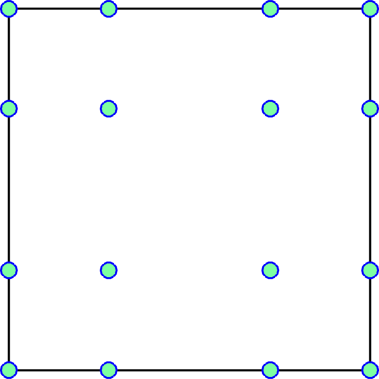
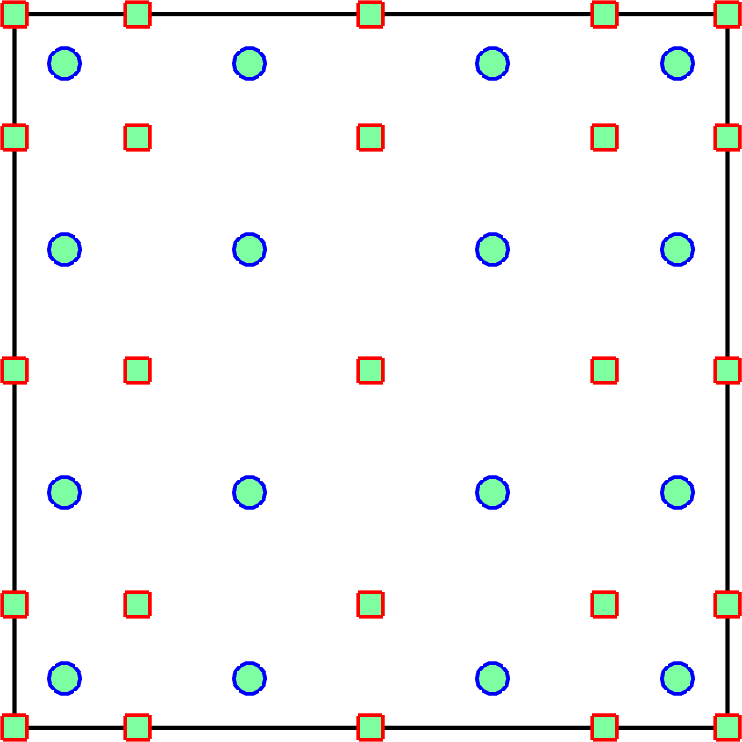
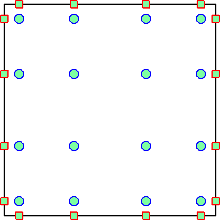
It is possible to realize the improved accuracy of Gauss points while avoiding non-compact SATs through a staggered grid formulation, where the solution is stored at Gauss nodes but interpolated to a set of higher degree $(N+2)$ GLL “flux” points for computation [parsani2016entropy]. Because GLL nodes include boundary points, compact and high order accurate SAT terms can be constructed for the flux points. After performing computations on the flux points, the results are interpolated back to Gauss points and used to evolve the solution forward in time. Figure 1 shows an illustration of GLL, staggered grid, and Gauss point sets for a 2D quadrilateral element.

The following sections will describe how to construct efficient high order entropy stable schemes using Gauss points. These schemes are based on “decoupled” SBP operators introduced in [chan2017discretely, chan2018discretely], which are applicable to general choices of basis and quadrature. By choosing a tensor product Lagrange polynomial basis and $(N+1)$ point Gauss quadrature rules, we recover a Gauss collocation scheme. The high order accuracy and entropy stability of this scheme are direct results of theorems presented in [chan2017discretely, chan2018discretely]. However, we will also present a different proof of entropy stability in one dimension for completeness.

3.1 Gauss nodes and generalized summation by parts operators

We assume the solution is collocated at $(N+1)$ quadrature points $x_{i}$ with associated quadrature weights $w_{i}$ . We do not make any assumptions on the points, in order to accommodate both GLL and Gauss nodes using this notation. The collocation assumption is equivalent to approximating the solution using a degree $N$ Lagrange basis $\ell_{j}(x)$ defined over the $(N+1)$ quadrature points.

Let $\bm{D}$ denote the nodal differentiation matrix, and let $\bm{V}_{f}$ denote the $2\times(N+1)$ matrix which interpolates polynomials at Gauss nodes to values at endpoints. These two matrices are defined entrywise as

\bm{D}_{ij}=\left.\frac{\partial\ell_{j}}{\partial x}\right|_{x=x_{i}},\qquad\left(\bm{V}_{f}\right)_{1i}=\ell_{i}(-1),\qquad\left(\bm{V}_{f}\right)_{2i}=\ell_{i}(1).

We also introduce the diagonal matrix of quadrature weights $\bm{W}_{ij}=\delta_{ij}w_{i}$ , as well as the one-dimensional mass matrix $\bm{M}$ whose entries are $L^{2}$ inner products of basis functions. We assume that these inner products are computed using the quadrature rule $(x_{i},w_{i})$ at which the solution is collocated. Under such an assumption, the mass matrix is diagonal with entries equal to the quadrature weights

\bm{M}_{ij}=\int_{-1}^{1}\ell_{i}(x)\ell_{j}(x)\approx\sum_{k=1}^{N+1}\ell_{i}(x_{k})\ell_{j}(x_{k})w_{k}=\delta_{ij}w_{i}=\bm{W}_{ij}.

Since $\bm{M}=\bm{W}$ under a collocation assumption, we utilize $\bm{W}$ for the remainder of this work to emphasize that the mass matrix is diagonal and related to the quadrature weights $w_{i}$ . The treatment of non-diagonal mass matrices is covered in [chan2017discretely, chan2018discretely].

It can be shown that the mass and differentiation matrices for Gauss nodes fall under the class of generalized SBP (GSBP) operators [fernandez2014generalized].

Lemma 3.1.

$\bm{Q}=\bm{W}\bm{D}$ satisfies the generalized summation by parts property

\bm{Q}=\bm{V}_{f}^{T}\bm{B}\bm{V}_{f}-\bm{Q}^{T},\qquad\bm{B}=\begin{bmatrix}-1&\\ &1\end{bmatrix}.

The proof is a direct restatement of integration by parts, and can be found in [fernandez2014generalized, ortleb2016kinetic, ortleb2017kinetic, ranocha2018generalised]. Lemma 3.1 holds for both GLL and Gauss nodes, and switching between these two nodal sets simply results in a redefinition of the matrices $\bm{D},\bm{V}_{f}$ . For example, because GLL nodes include boundary points, the interpolation matrix $\bm{V}_{f}$ reduces to a generalized permutation matrix which extracts the nodal values associated with the left and right endpoints.

3.2 Existing entropy stable SATs for generalized SBP operators

In this section, we will review the construction of semi-discretely entropy stable discretizations. Entropy stable discretizations can be constructed by first introducing an entropy conservative scheme, then adding appropriate interface dissipation to produce an entropy inequality. The construction of entropy conservative schemes relies on the existence of an two-point (dyadic) entropy conservative flux [tadmor1987numerical].

Definition 3.2.

Let $\bm{f}_{S}(\bm{u}_{L},\bm{u}_{R})$ be a bivariate function which is symmetric and consistent with the flux function $\bm{f}(\bm{u})$

\displaystyle\bm{f}_{S}(\bm{u}_{L},\bm{u}_{R})=\bm{f}_{S}(\bm{u}_{R},\bm{u}_{L}),\qquad\bm{f}_{S}(\bm{u},\bm{u})=\bm{f}(\bm{u})

The numerical flux $\bm{f}_{S}(\bm{u}_{L},\bm{u}_{R})$ is entropy conservative if, for entropy variables $\bm{v}_{L}=\bm{v}(\bm{u}_{L}),\bm{v}_{R}=\bm{v}(\bm{u}_{R})$ , the Tadmor “shuffle” condition is satisfied

\displaystyle\left(\bm{v}_{L}-\bm{v}_{R}\right)^{T}\bm{f}_{S}(\bm{u}_{L},\bm{u}_{R})=(\psi_{L}-\psi_{R}),\qquad\psi_{L}=\psi(\bm{v}(\bm{u}_{L})),\quad\psi_{R}=\psi(\bm{v}(\bm{u}_{R})).

For illustrative purposes, we will prove a semi-discrete entropy inequality on a one-dimensional mesh consisting of two elements of degree $N$ . We assume both meshes are translations of a reference element $[-1,1]$ , such that derivatives with respect to physical coordinates are identical to derivatives with respect to reference coordinates. The extension to multiple elements and variable mesh sizes is straightforward.

The construction of entropy conservative schemes relies on appropriate SATs for Gauss collocation schemes [fernandez2014review, crean2017high, fernandez2018simultaneous]. Let the rows of $\bm{V}_{f}$ be denoted by column vectors $\bm{t}_{L},\bm{t}_{R}$

\bm{V}_{f}=\begin{bmatrix}\left(\bm{t}_{L}\right)_{1},&\ldots,&\left(\bm{t}_{L}\right)_{N+1}\\ \left(\bm{t}_{R}\right)_{1},&\ldots,&\left(\bm{t}_{R}\right)_{N+1}\end{bmatrix},\qquad\left(\bm{t}_{L}\right)_{j}=\ell_{j}(-1),\qquad\left(\bm{t}_{R}\right)_{j}=\ell_{j}(1).

The inter-element coupling terms in [fernandez2014review, crean2017high, fernandez2018simultaneous] utilize a decomposition of the surface matrix $\bm{V}_{f}^{T}\bm{B}\bm{V}_{f}$ as

(4)

\bm{V}_{f}^{T}\bm{B}\bm{V}_{f}=\bm{t}_{R}\bm{t}_{R}^{T}-\bm{t}_{L}\bm{t}_{L}^{T}.

The construction of entropy conservative schemes on multiple elements requires appropriate inter-element coupling terms (SATs) involving $\bm{t}_{L},\bm{t}_{R}$ . We consider a two element mesh, and show how when coupled with SATs, the resulting discretization matrices can be interpreted as constructing a global SBP operator.

Let $\bm{u}^{1}_{N},\bm{u}^{2}_{N}$ denote nodal degrees of freedom of the vector valued solution $\bm{u}(x)$ on the first and second element, respectively. To simplify notation, we assume that all following operators are defined in terms of Kronecker products [chen2017entropy], such that they are applied to each component of $\bm{u}^{1}_{N},\bm{u}^{2}_{N}$ . We first define the matrix

(5)

\bm{S}\mathrel{\stackrel{{\scriptstyle\makebox[0.0pt]{\mbox{\tiny def}}}}{{=}}}\bm{Q}-\frac{1}{2}\bm{V}_{f}^{T}\bm{B}\bm{V}_{f}.

It is straightforward to show (using Lemma 3.1) that $\bm{S}$ is skew-symmetric. We can now define an SBP operator $\bm{D}_{h}=\bm{W}_{h}^{-1}\bm{Q}_{h}$ over two elements

(6)

\bm{Q}_{h}\mathrel{\stackrel{{\scriptstyle\makebox[0.0pt]{\mbox{\tiny def}}}}{{=}}}\underbrace{\begin{bmatrix}\bm{S}&\frac{1}{2}\bm{t}_{R}\bm{t}_{L}^{T}\\ -\frac{1}{2}\bm{t}_{L}\bm{t}_{R}^{T}&\bm{S}\end{bmatrix}}_{\bm{S}_{h}}+\underbrace{\begin{bmatrix}-\frac{1}{2}\bm{t}_{L}\bm{t}_{L}^{T}&\\ &\frac{1}{2}\bm{t}_{R}\bm{t}_{R}^{T}\end{bmatrix}}_{\frac{1}{2}\bm{B}_{h}},\qquad\bm{W}_{h}\mathrel{\stackrel{{\scriptstyle\makebox[0.0pt]{\mbox{\tiny def}}}}{{=}}}\begin{bmatrix}\bm{W}&\\ &\bm{W}\end{bmatrix}.

It can be shown that $\bm{D}_{h}$ is high order accurate such that, if $\bm{u}_{h}$ is a polynomial of degree $N$ , it is differentiated exactly. Straightforward computations show that $\bm{Q}_{h}$ also satisfies an SBP property $\bm{Q}_{h}+\bm{Q}_{h}^{T}=\bm{B}_{h}$ .

Ignoring boundary conditions, an entropy conservative scheme for (1) on two elements can then be given as

(7)		$\displaystyle\frac{{\rm d}}{{\rm d}{\rm t}}\bm{W}_{h}\bm{u}_{h}+2\left(\bm{Q}_{h}\circ\bm{F}_{S}\right)\bm{1}=0,\qquad\bm{u}_{h}=\begin{bmatrix}\bm{u}^{1}_{N}\\ \bm{u}^{2}_{N}\end{bmatrix}$
	$\displaystyle\left(\bm{F}_{S}\right)_{ij}=\bm{f}_{S}\left(\left(\bm{u}_{h}\right)_{i},\left(\bm{u}_{h}\right)_{j}\right),\qquad 1\leq i,j\leq 2(N+1),$

where $\circ$ denotes the Hadamard product [horn2012matrix]. It should be emphasized that here, $(\bm{u}_{h})_{i},(\bm{u}_{h})_{j}$ denote vectors containing solution components at nodes $i,j$ , and that (because $\bm{f}_{S}$ is a vector-valued flux) the term $\left(\bm{F}_{S}\right)_{ij}$ should be interpreted as a diagonal matrix whose diagonal entries consist of the components of $\bm{f}_{S}\left((\bm{u}_{h})_{i},(\bm{u}_{h})_{j}\right)$ .

Multiplying (7) by $\bm{v}_{h}^{T}=\bm{v}\left(\bm{u}_{h}\right)^{T}$ will yield a semi-discrete version of the conservation of entropy (mimicking (3) with the inequality replaced by an equality)

(8)

\frac{{\rm d}}{{\rm d}{\rm t}}\bm{W}_{h}S(\bm{u}_{h})+\bm{v}_{h}^{T}\left(\bm{B}_{h}\circ\bm{F}_{S}\right)\bm{1}-\bm{1}^{T}\bm{B}_{h}\psi\left(\bm{u}_{h}\right)=0.

We refer to [crean2017high, crean2018entropy] for the proof of (8).

The drawback of the SATs introduced in this section lies in the nature of the off-diagonal matrices $\bm{t}_{R}\bm{t}_{L}$ and $-\bm{t}_{L}\bm{t}_{R}$ . For Gauss nodes, these blocks are dense, which implies that inter-element coupling terms produce a non-compact stencil. Evaluating (7) requires computing two-point fluxes $\bm{f}_{S}$ between all nodes on two neighboring elements, which significantly increases both the computational work, as well as communication between neighboring elements. This leads to all-to-all coupling between degrees of freedom in 1D, and to coupling along one-dimensional lines of nodes in higher dimensions due to the tensor product structure.

The main goal of this work is to circumvent this tighter coupling of degrees of freedom introduced by the SATs described in this section, which can be done through the use of “decoupled” SBP operators.

3.3 Decoupled SBP operators

Decoupled SBP operators were first introduced in [chan2017discretely] and used to construct entropy stable schemes on simplicial elements. These operators (and simplifications under a collocation assumption) are presented in a more general setting in [chan2017discretely, chan2018discretely] and in Appendix LABEL:app:decoupled. In this section, decoupled SBP operators are introduced in one dimension for GLL and Gauss nodal sets.

Decoupled SBP operators build upon the GSBP matrices $\bm{W},\bm{Q}$ , interpolation matrix $\bm{V}_{f}$ , and boundary matrix $\bm{B}$ introduced in Section 3.1. The decoupled SBP operator $\bm{Q}_{N}$ is defined as the block matrix

(9)

\bm{Q}_{N}\mathrel{\stackrel{{\scriptstyle\makebox[0.0pt]{\mbox{\tiny def}}}}{{=}}}\begin{bmatrix}\bm{Q}-\frac{1}{2}\bm{V}_{f}^{T}\bm{B}\bm{V}_{f}&\frac{1}{2}\bm{V}_{f}^{T}\bm{B}\\ -\frac{1}{2}\bm{B}\bm{V}_{f}&\frac{1}{2}\bm{B}\end{bmatrix}.

Lemma 3.1 and straightforward computations show that $\bm{Q}_{N}$ also satisfies the following SBP property

Lemma 3.3.

Let $\bm{Q}_{N}$ be defined through (9). Then,

\bm{Q}_{N}+\bm{Q}_{N}^{T}=\begin{bmatrix}\bm{0}&\\ &\bm{B}\end{bmatrix}.

We note that the matrix $\bm{Q}_{N}$ acts not only on volume nodes, but on both volume and surface nodes. Thus, it is not immediately clear how to apply this operator to GSBP discretizations of nonlinear conservation laws. It is straightforward to evaluate the nonlinear flux at volume nodes since the solution is collocated at these points; however, evaluating the nonlinear flux at surface nodes is less straightforward. Moreover, $\bm{Q}_{N}$ does not directly define a difference operator, and must be combined with another operation to produce an approximation to the derivative. We will discuss how to apply $\bm{Q}_{N}$ in two steps. First, we will show how to approximate the derivative of an arbitrary function using $\bm{Q}_{N}$ given function values at both volume and surface nodes. Then, we will describe how to apply this approximation to compute derivatives of nonlinear flux functions given collocated solution values at volume nodes.

Let $f(x),g(x)$ denote two functions, and let $\bm{f},\bm{g}$ denote the values of $f,g$ at interior nodal points. We also define vectors $\bm{f}_{N},\bm{g}_{N}$ denoting the values of $f,g$ at both interior and boundary points

(10)

\bm{f}_{N}=\begin{bmatrix}f\left(x_{1}\right)\\ \vdots\\ f\left(x_{N+1}\right)\\ f(-1)\\ f(1)\end{bmatrix}=\begin{bmatrix}\bm{f}\\ \bm{f}_{f}\end{bmatrix},\qquad\bm{g}_{N}=\begin{bmatrix}g\left(x_{1}\right)\\ \vdots\\ g\left(x_{N+1}\right)\\ g(-1)\\ g(1)\end{bmatrix}=\begin{bmatrix}\bm{g}\\ \bm{g}_{f}\end{bmatrix}.

Then, a polynomial approximation to $f\frac{\partial g}{\partial x}$ can be computed using $\bm{Q}_{N}$ . Let $\bm{u}$ denote the nodal values of the polynomial $u(x)\approx f\frac{\partial g}{\partial x}$ . These coefficients are computed via

(11)

\bm{W}\bm{u}=\begin{bmatrix}\bm{I}\\ \bm{V}_{f}\end{bmatrix}^{T}{\rm diag}\left(\bm{f}_{N}\right)\bm{Q}_{N}\bm{g}_{N}.

The approximation (11) can be rewritten in “strong” form as follows

	$\displaystyle\bm{u}=\bm{W}^{-1}\begin{bmatrix}\bm{I}\\ \bm{V}_{f}\end{bmatrix}^{T}$	$\displaystyle{\rm diag}\left(\bm{f}_{N}\right)\bm{Q}_{N}\bm{g}_{N}$
	$\displaystyle={\rm diag}\left(\bm{f}\right)\bm{D}\bm{g}$	$\displaystyle+\frac{1}{2}{\rm diag}\left(\bm{f}\right)\bm{W}^{-1}\bm{V}_{f}^{T}\bm{B}\left(\bm{g}_{f}-\bm{V}_{f}\bm{g}\right)$
		$\displaystyle+\frac{1}{2}\bm{W}^{-1}\bm{V}_{f}^{T}\bm{B}{\rm diag}\left(\bm{f}_{f}\right)\left(\bm{g}_{f}-\bm{V}_{f}\bm{g}\right),$

where we have used the fact that diagonal matrices commute to simplify expressions. The decoupled SBP operator $\bm{Q}_{N}$ can thus be interpreted as adding boundary corrections to the GSBP operator $\bm{D}$ in a skew-symmetric fashion.

Note 3.4.

More specifically, the expression (11) corresponds to a quadrature approximation of the following variational approximation of the derivative [chan2017discretely]: find $u\in P^{N}([-1,1])$ such that,