Graph-based Deep-Tree Recursive Neural Network (DTRNN) for Text Classification

Abstract

A novel graph-to-tree conversion mechanism called the deep-tree generation (DTG) algorithm is first proposed to predict text data represented by graphs. The DTG method can generate a richer and more accurate representation for nodes (or vertices) in graphs. It adds flexibility in exploring the vertex neighborhood information to better reflect the second order proximity and homophily equivalence in a graph. Then, a Deep-Tree Recursive Neural Network (DTRNN) method is presented and used to classify vertices that contains text data in graphs. To demonstrate the effectiveness of the DTRNN method, we apply it to three real-world graph datasets and show that the DTRNN method outperforms several state-of-the-art benchmarking methods.

Index Terms—  Natural Language Processing, Recursive Neural Network, Graph Data Processing, Artificial Neural Networks

1 Introduction

Research on natural languages in graph representation has gained more interests because many speech/text data in social networks and other multi-media domains can be well represented by graphs. These data often come in high-dimensional irregular form which makes them more difficult to analyze than the traditional low-dimensional corpora data. Node (or vertex) prediction is one of the most important tasks in graph analysis. Predicting tasks for nodes in a graph deal with assigning labels to each vertex based on vertex contents as well as link structures. Researchers have proposed different techniques to solve this problem and obtained promising results using various machine learning methods. However, research on generating an effective tree-structure to best capture connectivity and density of nodes in a network is still not yet extensively conducted.

In our proposed architecture, the input text data come in form of graphs. Graph features are first extracted and converted to tree structure data using our deep-tree generation (DTG) algorithm. Then, the data is trained and classified using the deep-tree recursive neural network (DTRNN). The process generates a class prediction for each node in the graph as the output. The workflow of the DTRNN algorithm is shown in Figure 1.

There are two major contributions of this work. First, we propose a graph-to-tree conversion mechanism and call it the DTG algorithm. The DTG algorithm captures the structure of the original graph well, especially on its second order proximity. The second-order proximity between vertices is not only determined by observed direct connections but also shared neighborhood structures of vertices [1]. To put it another way, nodes with shared neighbors are likely to be similar. Next, we present the DTRNN method that brings the merits of the Long Short-Term Memory (LSTM) network [2] and the deep tree representation together. The proposed DTRNN method not only conserves the link feature better but also includes the impact feature of nodes with more outgoing and incoming edges. It extends the tree-structured RNN and models the long-distance vertex relation on more representative sub-graphs to offer the state-of-the-art performance as demonstrated in our conducted experiments. An in-depth analysis on the impact of the attention mechanism and runtime complexity of our method is also provided. .

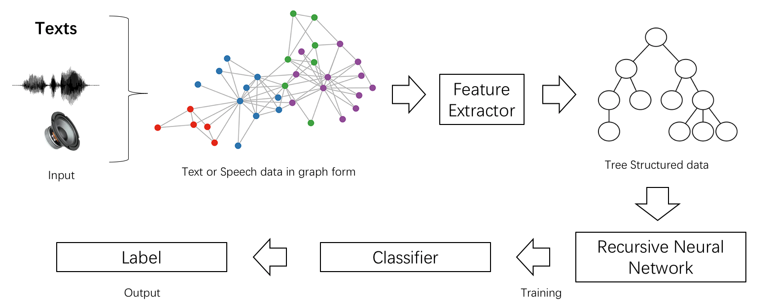
Fig. 1: The workflow of the DTRNN algorithm.

The rest of this paper is organized as follows. Related previous work is reviewed in Sec. 2. Both the DTRNN algorithm and the DTG algorithm are described in Sec. 3. The impact of the attention model is discussed in Sec. 4. The experimental results and their discussion are provided in Sec. 5. Finally, concluding remarks are given in Sec. 6.

2 Review of Related Work

Structures in social networks are non-linear in nature. Network structure understanding can benefit from modern machine learning techniques such as embedding and recursive models. Recent studies, such as DeepWalk [3] and node2vec [4], aim at embedding large social networks to a low-dimensional space. For example, the Text-Associated DeepWalk (TADW) method [5] uses matrix factorization to generate structural and vertex feature representation. However, these methods do not fully exploit the label information in the representation learning. As a result, they might not offer the optimal result.

Another approach to network structure analysis is to leverage the recursive neural network (RNN). The Recursive Neural Tensor Network (RNTN) [6] was demonstrated to be effective in training non-linear data structures. The Graph-based Recurrent Neural Network (GRNN) [7] utilizes the RNTN based on local sub-graphs generated from the original network structure. These sub-graphs are generated via breadth-first search with a depth of at most two. Later, the GRNN is improved by adding an attention layer in the Attention Graph-based Recursive Neural Network (AGRNN) [8]. Motivated by the GRNN and AGRNN models, we propose a new solution in this work, called the Deep-tree Recursive Neural Network (DTRNN), to improve the node prediction performance furthermore.

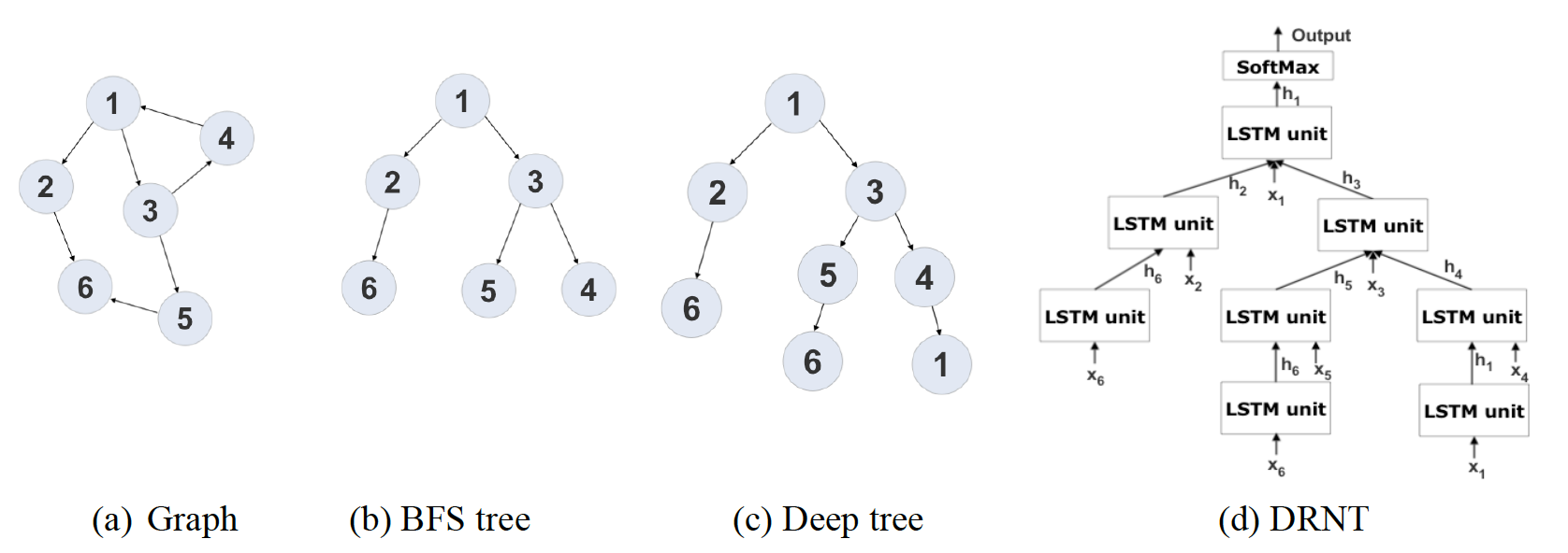
Fig. 2: (a) The graph to be converted into a tree, (b) the tree converted to a sub-graph using breadth-first search, (c) the tree converted using the deep-tree generation method (our method), and (d) the DTRNN constructed from the tree with LSTM units.

3 Proposed Methodology

3.1 Deep-Tree Recursive Neural Network (DTRNN) Algorithm

A graph denoted by $G=(V,E)$ consists of a set of vertices, $V=\{v_{1},v_{2},...,v_{n}\}$, and a set of edges, $E=\{e_{i,j}\}$, where edge $e_{i,j}$ connects vertex $v_{i}$ to vertex $v_{j}$. Let $X_{i}=\{x_{1},x_{2},...,x_{n}\}$ be the feature vector associated with vertex $v_{i}$, $l_{i}$ be the label or class that $v_{i}$ is assigned to and $L$ the set of all labels. The node prediction task attempts to find an appropriate label for any vertex $v_{t}$ so that the probability of given vertex $v_{k}$ with label $l_{k}$ is maximized. Mathematically, we have

$$\hat{l_{k}}=\operatorname*{arg\,max}_{l_{k}\in L}P_{\theta}(l_{k}|v_{k},G).$$ (1)

A softmax classifier is used to predict label $l_{k}$ of the target vertex $v_{k}$ using its hidden states $h_{k}$

$$P_{\theta}(l_{k}|v_{k},G)={\rm softmax}(W_{s}h_{k}+b_{s})$$ (2)

where $\theta$ denotes model parameters. Typically, the negative log likelihood criterion is used as the cost function. For a network of $N$ vertices, its cross-entropy is defined as

$$J(\theta)=-\frac{1}{N}\sum_{k=1}^{N}\log P_{\theta}(l_{k}|v_{k},G).$$ (3)

To solve the graph node classification problem, we use the Child-Sum Tree-LSTM [9] data structure to represent the node and link information in a graph. Based on input vectors of target vertex’s child nodes, the Tree-LSTM generates a vector representation for each target node in the dependency tree. Like the standard LSTM, each node $v_{k}$ has a forget gate, denoted by $f_{kr}$, to control the memory flow amount from $v_{k}$ to $v_{r}$; input and output gates $i_{k}$ and $o_{k}$, where each of these gates acts as a neuron in the feed-forward neural network, $f_{kr}$ $i_{k}$ and $o_{k}$ represent the activation of the forget gate, input and output gates, respectively; hidden states $h_{k}$ for representation of the node (output vector in the LSTM unit, and memory cells); $c_{k}$ that indicates the cell state vector. Each child takes on input $x_{k}$ which is the vector representation of child nodes.

As a result, the DTRNN method can be summarized as:

$$\hat{h_{k}} =\max\{h_{r}\},$$ (4a)

$$f_{kr} =\sigma(W_{f}x_{k}+U_{f}h_{c}+b_{f}),$$ (4b)

$$i_{k} =\sigma(W_{i}x_{k}+U_{i}\hat{h_{k}}+b_{i}),$$ (4c)

$$o_{k} =\sigma(W_{o}x_{k}+U_{o}\hat{h_{k}}+b_{o}),$$ (4d)

$$u_{k} =\tanh(W_{u}x_{k}+U_{u}\hat{h_{k}}+b_{u}),$$ (4e)

$$c_{k} =i_{k}\circ u_{k}+\sum\limits_{v_{r}\in C(v_{k})}f_{kr}\circ c_{r},$$ (4f)

$$h_{k} =o_{k}\circ\tanh(c_{k}).$$ (4g)

In the equations above, $\circ$ and $\sigma$ denote the element-wise multiplication and the sigmoid function, $W_{f}$, $W_{i}$, $W_{o}$ are the weights between the forget layer and forget gate, the input layer and the input gate, the forget gate and the output gate; $U_{f}$, $U_{i}$, $U_{o}$ are the weights between the hidden recurrent layer and the forget gate, the input gate and the output gate of the memory block; $b_{f}$, $b_{i}$, $b_{o}$ are the additive biases of the forget gate, the input gate and the output gate, respectively.

The DTRNN is trained with back propagation through time [10]. The model parameters are randomly initialized. In the training process, the weight are updated after the input has been propagated forward in the network. The error is calculated using the negative log likelihood criterion.

3.2 Deep-Tree Generation (DTG) Algorithm

In [11], a graph was converted to a tree using a breadth-first search algorithm with a maximum depth of two. However, it fails to capture long-range dependency in the graph so that the long short-term memory in the Tree-LSTM structure cannot be fully utilized. The main contribution of this work is to generate a deep-tree representation of a target node in a graph. The generation starts at the target/root node. At each step, a new edge and its associated node are added to the tree. The deep-tree generation strategy is given in Algorithm 1. This process can be well explained using an example given in Figure 2.

Algorithm 1 Deep-Tree Generation Algorithm

Input: $G$, $u_{i}$, maxCount

TreeGeneration (Graph $G$, Node $u_{i}$, maxCount)

Initialize walk to a queue $Q=$ [$u_{i}$]

While $Q$ is not empty and

totalNode $<$ maxCount do

$v_{c}=Q$.pop()

if $v$.child exists then

for $w$ in G.outVertex(v) do

add $w$ as the child of $v$

$Q$.push($w$)

end for

end if

end while

return T

Currently, the most common way to construct a tree is to traverse the graph using the breadth first search (BFS) method. The BFS method starts at the tree root. It explores all immediate children nodes first before moving to the next level of nodes until the termination criterion is reached. For the graph given in Figure 2(a), it is clear that node $v_{5}$ is connected to $v_{6}$ via $e_{5,6}$, and the shortest distance from $v_{4}$ to $v_{6}$ is three hops; namely, through $e_{4,1}$,$e_{1,2}$ and $e_{2,6}$. For the BFS tree construction process as shown in Figure 2(b), we see that such information is lost in the translation. On the other hand, if we construct a tree by incorporating the deepening depth first search, which is a depth limited version of the depth first search [12], as shown in Algorithm 1, we are able to recover the connection from $v_{5}$ to $v_{6}$ and get the correct shortest hop from $v_{4}$ to $v_{6}$ as shown in Figure 2(c). Apparently, the deep-tree construction strategy preserves the original neighborhood information better. The maximum number for a node to appear in a constructed tree is bounded by its total in- and out-degrees. This is consistent with our intuition that a node with more outgoing and incoming edges tends to have a higher impact on its neighbors.

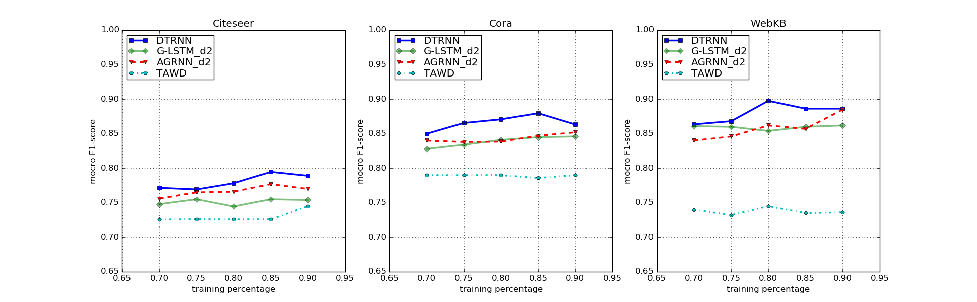
Fig. 3: Comparison of four methods on three data sets (from left to right): Citeseer, Cora and WebKB, where the x-axis is the percentage of training data and the y-axis is the average Macro-F1 score.

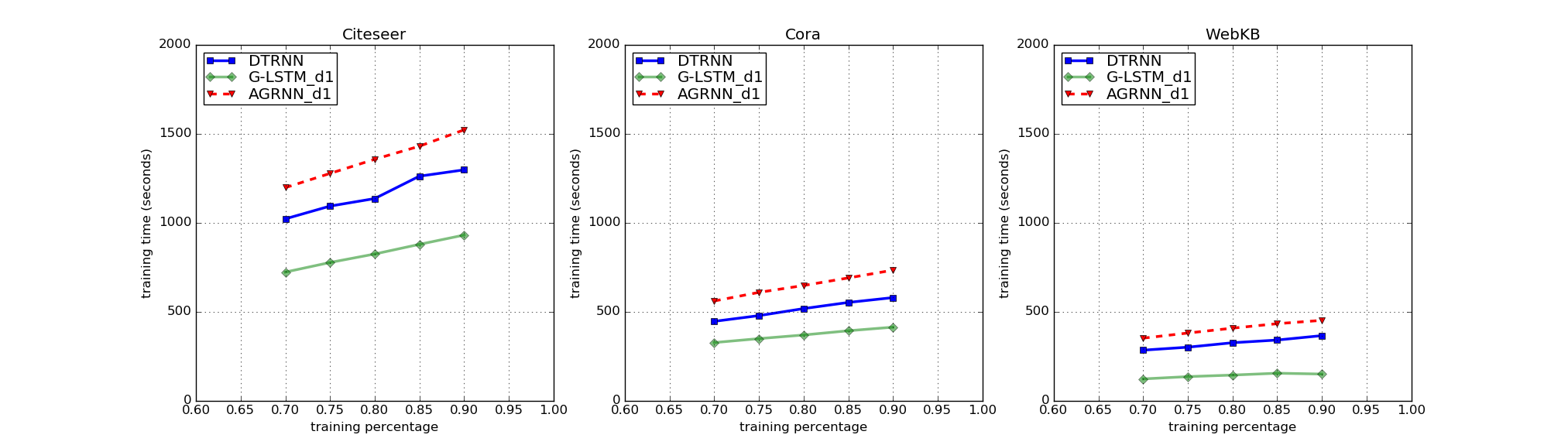
Fig. 4: Comparison of runtime for three data sets (from left to right): Citeseer, Cora and WebKB, where the x-axis is the percentage of training data and the y-axis is the runtime in seconds.

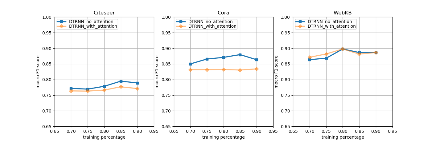
Fig. 5: Performance comparison of DTRNN with and without the soft attention layer (from left to right: Citeseer, Cora and WebKB), where the x-axis is the percentage of training data and the y-axis is the average Macro-F1 score.

4 Impact of Attention Model

An attentive recursive neural network can be adapted from a regular recursive neural network by adding an attention layer so that the new model focuses on the more relevant input. The attentive neural network has demonstrated improved performance in machine translation, image captioning, question answering and many other different machine learning fields. The added attention layer might increase the classification accuracy because the graph data most of the time contain noise. The less irrelevant neighbors should has less impact on the target vertex than the neighbors that are more closely related to the target vertex. Attention models demonstrated improved accuracy in several applications.

In this work, we examine how the added attention layers could affect the results of our model. In the experiment, we added an attention layer to see whether the attention mechanism could help improve the proposed DTRNN method. The attention model is taken from [8] that aims to differentiate the contribution from a child vertex to a target vertex using a soft attention layer. It determines the attention weight, $\alpha_{r}$, using a parameter matrix denoted by $W_{\alpha}$. Matrix $W_{\alpha}$ is used to measure the relatedness of $x$ and $h_{r}$. It is learned by the gradient descent method in the training process. The softmax function is used to set the sum of attention weights to equal 1. The aggregated hidden state of the target vertex is represented as the summation of all the soft attention weight times the hidden states of child vertices as

$$\alpha_{r}={\rm Softmax}(x^{T}W_{\alpha}h_{r}),$$ (5)

where

$$\hat{h_{r}}=\alpha_{r}h_{r}.$$ (6)

Based on Eqs. 4(a), (5) and (6), we can obtain

$$\hat{h_{k}}=\max{\{{\rm Softmax}(x^{T}W_{\alpha}h_{r})h_{r}\}}.$$ (7)

Athough the attention model can improve the overall accuracy of a simple-tree model generated by a graph, its addition does not help but hurts the performance of the proposed deep-tree model. This could be attributed to several reasons.

It is obvious to see that $\alpha_{r}$ is bounded between 0 and 1 because of the softmax function. If one target root has more child nodes, $\alpha_{r}$ will be smaller and getting closer to zero. By comparing Figures 2(b) and (c), we see that nodes that are further apart will have vanishing impacts on each other under this attention model since our trees tend to have longer paths. The performance comparision of DTRNN with and without attention added is given in Figure 5. For Cora, we see that DTRNN without the attention layer outperforms the one with attention layer by 1.8-3.7%. For Citeseer, DTRNN without the attention layer outperforms by 0.8-1.9%. For WebKB, the performance of the two are about the same.

Furthermore, this attention model pays close attention to the immediate neighbor of a target yet ignores the second-order proximity, which can be interpreted as nodes with shared neighbors being likely to be similar [1]. Prediction tasks on nodes in networks should take care of two types of similarities: (1) homophily and (2) structural equivalence [13]. The homophily hypothesis [14] states that nodes that are highly interconnected and belong to similar network clusters or communities should be similar to each other. The vanishing impact of scalded $h_{r}$ tends to reduce these features in our graph. In the next section, we will show by experiments that the DTRNN method without the attention model outperforms a tree generated by the traditional BFS method with an attention LSTM unit and also DTRNN method with attention model .

5 Experiments

5.1 Datasets

To evaluate the performance of the proposed DTRNN method, we used the following two citation and one website datasets in the experiment.

• Citeseer: The Citeseer dataset is a citation indexing system that classifies academic literature into 6 categories [15]. This dataset consists of 3,312 scientific publications and 4,723 citations.

• Cora: The Cora dataset consists of 2,708 scientific publications classified into seven classes [16]. This network has 5,429 links, where each link is represented by a 0/1-valued word vector indicating the absence/presence of the corresponding word from a dictionary consists of 1,433 unique words.

• WebKB: The WebKB dataset consists of seven classes of web pages collected from computer science departments: student, faculty, course, project, department, staff and others [17]. It consists of 877 web pages and 1,608 hyper-links between web pages.

5.2 Experimental Settings

These three datasets are split into training and testing sets with proportions varying from 70% to 90%. We run 10 epochs on the training data and recorded the highest and the average Micro-F1 scores for items in the testing set.

5.3 Baselines

We implemented a DTRNN consisting of 200 hidden states, and compare its performance with that of three benchmarking methods, which are described below.

• Text-associated Deep Walk (TADW). It incorporates text features of vertices under the matrix factorization framework [5] for vertex classification.

• Graph-based LSTM (G-LSTM). It first builds a simple tree using the BFS only traversal and, then, applies an LSTM to the tree for vertex classification [7].

• Attentive Graph-based Recursive Neural Network (AGRNN). It is improved upon the GRNN with soft attention weight added in the each attention unit as depicted in Eqs. (5) and (6) [8].

5.4 Results and Analysis

The Macro-F1 scores of all four methods for the above-mentioned three datasets are compared in Figure 5. We see that the proposed DTRNN method consistently outperforms all benchmarking methods. When comparing the DTRNN and the AGRNN, which has the best performance among the three benchmarks, the DTRNN has a gain up to 4.14%. The improvement is the greatest on the WebKB dataset. In the Cora and the Citeseer datasets, neighboring vertices tend to share the same label. In other words, labels are closely correlated among short range neighbors. In the WebKB datasets, this short range correlation is not as obvious, and some labels are strongly related to more than two labels [7]. Since our tree-tree generation strategy captures the long distance relation among nodes, we see the largest improvement in this dataset.

5.5 Complexity Analysis

The graph-to-tree conversion is relatively fast. For both the breadth-first and our method, the time complexity to generate the tree is $b^{d}$, where $b$ is the max branching factor of the tree, and $d$ is the depth. The DTRNN algorithm builds a longer tree with more depth. Thus, the tree construction and training will take longer yet overall it still grows linearly with the number of input node asymptotically.

The bottleneck of the experiments was the training process. During each training time step, the time complexity for updating a weight is $O(1)$. Then, the overall LSTM algorithm has an update complexity of $O(W)$ per time step, where $W$ is the number of weights [2] that need to be updated. In addition, LSTM is local in space and time, meaning that it does not depend on the network size to update complexity per time step and weight, and the storage requirement does not depend on input sequence length [18]. For the whole training process, the run time complexity is $O(Wie)$, where $i$ is the input length and $e$ is the number of epochs.

In our experiments, the input length is fixed per time step because the hidden states of the child vertices are represented by max pooling of all children’s inputs. The number of epochs is fixed at 10. The actual running time for each data set is recorded for the DTRNN method and the G-LSTM method. The results are shown in Figure 3. If attention layers are added as described in the earlier section, they come at a higher cost. The attention weights need to be calculated for each combination of child and target vertex. If we have $c$ children on average for $n$ target vertices, there will be $c\times n$ attention values. The actual machine runtime of three datasets are shown in Figure 4. The CPU runtime shows that the DTRRN is faster than the AGRNN-d1 (with an attention model of depth equal to 1) by 20.59% for WebKB, 14.78% for Citeseer, and 21.06% for Cora while having the highest classification accuracy among all three methods.

6 Conclusion and Future Work

A novel strategy to convert a social citation graph to a deep tree and to conduct the vertex classification problem was proposed in this work. It was demonstrated that the proposed deep-tree generation (DTG) algorithm can capture the neighborhood information of a node better than the traditional breath first search tree generation method. Experimental results on three citation datasets with different training ratios proved the effectiveness of the proposed DTRNN method. That is, our DTRNN method offers the state-of-the-art classification accuracy for graph structured text.

We also trained graph data in the DTRNN by adding more complex attention models, yet attention models does not generate better accuracy because our DTRNN algorithm alone already captures more features of each node. The complexity of the proposed method was analyzed. We considered both asymptotic run time and real time CPU runtime and showed that our algorithm is not only the most accurate but also very efficient.

In the near future, we would like to apply the proposed methodology to graphs of a larger scale and higher diversity such as social network data. Furthermore, we will find a new and better way to explore the attention model although it does not help much in our current implementation.

References

- [1] Jian Tang, Meng Qu, Mingzhe Wang, Ming Zhang, Jun Yan, and Qiaozhu Mei, “Line: Large-scale information network embedding,” in Proceedings of the 24th International Conference on World Wide Web. International World Wide Web Conferences Steering Committee, 2015, pp. 1067–1077.
- [2] Sepp Hochreiter and Jürgen Schmidhuber, “Long short-term memory,” Neural computation, vol. 9, no. 8, pp. 1735–1780, 1997.
- [3] Bryan Perozzi, Rami Al-Rfou, and Steven Skiena, “Deepwalk: Online learning of social representations,” in Proceedings of the 20th ACM SIGKDD international conference on Knowledge discovery and data mining. ACM, 2014, pp. 701–710.
- [4] Aditya Grover and Jure Leskovec, “node2vec: Scalable feature learning for networks,” in Proceedings of the 22nd ACM SIGKDD international conference on Knowledge discovery and data mining. ACM, 2016, pp. 855–864.
- [5] Cheng Yang, Zhiyuan Liu, Deli Zhao, Maosong Sun, and Edward Y Chang, “Network representation learning with rich text information.,” in IJCAI, 2015, pp. 2111–2117.
- [6] Richard Socher, Alex Perelygin, Jean Wu, Jason Chuang, Christopher D Manning, Andrew Ng, and Christopher Potts, “Recursive deep models for semantic compositionality over a sentiment treebank,” in Proceedings of the 2013 conference on empirical methods in natural language processing, 2013, pp. 1631–1642.
- [7] Qiongkai Xu, Qing Wang, Chenchen Xu, and Lizhen Qu, “Collective vertex classification using recursive neural network,” arXiv preprint arXiv:1701.06751, 2017.
- [8] Qiongkai Xu, Qing Wang, Chenchen Xu, and Lizhen Qu, “Attentive graph-based recursive neural network for collective vertex classification,” in Proceedings of t he 2017 ACM on Conference on Information and Knowledge Management. ACM, 2017, pp. 2403–2406.
- [9] Kai Sheng Tai, Richard Socher, and Christopher D Manning, “Improved semantic representations from tree-structured long short-term memory networks,” arXiv preprint arXiv:1503.00075, 2015.
- [10] Paul J Werbos, “Backpropagation through time: what it does and how to do it,” Proceedings of the IEEE, vol. 78, no. 10, pp. 1550–1560, 1990.
- [11] Sunghwan Mac Kim, Qiongkai Xu, Lizhen Qu, Stephen Wan, and Cécile Paris, “Demographic inference on twitter using recursive neural networks,” in Proceedings of the 55th Annual Meeting of the Association for Computational Linguistics (Volume 2: Short Papers), 2017, vol. 2, pp. 471–477.
- [12] Michael T Goodrich and Roberto Tamassia, Algorithm design: foundation, analysis and internet examples, John Wiley & Sons, 2006.
- [13] Peter D Hoff, Adrian E Raftery, and Mark S Handcock, “Latent space approaches to social network analysis,” Journal of the american Statistical association, vol. 97, no. 460, pp. 1090–1098, 2002.
- [14] Jaewon Yang and Jure Leskovec, “Overlapping communities explain core–periphery organization of networks,” Proceedings of the IEEE, vol. 102, no. 12, pp. 1892–1902, 2014.
- [15] C Lee Giles, Kurt D Bollacker, and Steve Lawrence, “Citeseer: An automatic citation indexing system,” in Proceedings of the third ACM conference on Digital libraries. ACM, 1998, pp. 89–98.
- [16] Andrew Kachites McCallum, Kamal Nigam, Jason Rennie, and Kristie Seymore, “Automating the construction of internet portals with machine learning,” Information Retrieval, vol. 3, no. 2, pp. 127–163, 2000.
- [17] Mark Craven, Andrew McCallum, Dan PiPasquo, Tom Mitchell, and Dayne Freitag, “Learning to extract symbolic knowledge from the world wide web,” 1998.
- [18] Jurgen Schmidhuber, “A local learning algorithm for dynamic feedforward and recurrent networks,” Connection Science, vol. 1, no. 4, pp. 403–412, 1989.