$t$-Exponential Memory Networks for Question-Answering Machines

Abstract

Recent advances in deep learning have brought to the fore models that can make multiple computational steps in the service of completing a task; these are capable of describing long-term dependencies in sequential data. Novel recurrent attention models over possibly large external memory modules constitute the core mechanisms that enable these capabilities. Our work addresses learning subtler and more complex underlying temporal dynamics in language modeling tasks that deal with sparse sequential data. To this end, we improve upon these recent advances, by adopting concepts from the field of Bayesian statistics, namely variational inference. Our proposed approach consists in treating the network parameters as latent variables with a prior distribution imposed over them. Our statistical assumptions go beyond the standard practice of postulating Gaussian priors. Indeed, to allow for handling outliers, which are prevalent in long observed sequences of multivariate data, multivariate $t$-exponential distributions are imposed. On this basis, we proceed to infer corresponding posteriors; these can be used for inference and prediction at test time, in a way that accounts for the uncertainty in the available sparse training data. Specifically, to allow for our approach to best exploit the merits of the $t$-exponential family, our method considers a new $t$-divergence measure, which generalizes the concept of the Kullback-Leibler divergence. We perform an extensive experimental evaluation of our approach, using challenging language modeling benchmarks, and illustrate its superiority over existing state-of-the-art techniques.

I Introduction

Recent developments in machine learning have managed to achieve breakthrough improvements in modeling long-term dependencies in sequential data. Specifically, the machine learning community has recently witnessed a resurgence in models of computation that use explicit storage and a notion of attention [1, 2, 3, 4]. As it has been extensively shown, the capability of effectively manipulating such storage mechanisms offers a very potent solution to the problem of modeling long temporal dependencies. Its advantages have been particularly profound in the context of question-answering bots. In such applications, it is required that the trained models be capable of taking multiple computational steps in the service of answering a question or completing a related task.

This work builds upon these developments, seeking novel treatments of Memory Networks (MEM-NNs) [2, 3] to allow for more flexible and effective learning from sparse sequential data with heavy-tailed underlying densities. Indeed, both sparsity and heavy tails are salient characteristics in a large variety of real-world language modeling tasks. Specifically, the earliest solid empirical evidence that any sufficiently large corpus of natural language utterances entails heavy-tailed distributions with power-law nature dates back to 1935 [5]. Hence, we posit that the capability of better addressing these data properties might allow for advancing the state-of-the-art in the field. Our inspiration is drawn from recent developments in approximate Bayesian inference for deep learning models [6, 7, 8, 9, 10]. Bayesian inference in the context of deep learning models can be performed by considering that the network parameters are stochastic latent variables with some prior distribution imposed over them. This inferential framework allows for the developed network to account for the uncertainty in the available (sparse) training data. Thus, it is expected to yield improved predictive and inferential performance outcomes compared to the alternatives.

Existing Bayesian inference formulations of deep networks postulate Gaussian assumptions regarding the form of the imposed priors and corresponding (inferred) posterior distributions. Then, inference can be performed in an approximate, computationally efficient way, by resorting to variational Bayes [11]. This consists in searching for a proxy in an analytically solvable distribution family that approximates the true underlying distribution. To measure the closeness between the true and the approximate distribution, the relative entropy between these two distributions is used. Specifically, under the aforementioned Gaussian assumption, one can use the Shannon-Boltzmann-Gibbs (SBG) entropy, whereby the relative entropy yields the well known Kullback-Leibler (KL) divergence [12].

Despite these advances, in problems dealing with long sequential data comprising multivariate observations, such assumptions of normality are expected to be far from the actual underlying densities. Indeed, it is well-known that real-world multivariate sequential observations tend to entail a great deal of outliers (heavy-tailed nature). This fact gives rise to significant difficulties in data modeling, the immensity of which increases with the dimensionality of the data [13]. Hence, replacing the typical Gaussian assumption with alternatives has been recently proposed as a solution towards the amelioration of these issues [14].

Our work focuses on the $t$-exponential family, which was first proposed by Tsallis and co-workers [15, 16, 17], and constitutes a special case of the more general $\phi$-exponential family [18, 19, 20]. Of specific practical interest to us is the Students’-$t$ density, which has been extensively examined in the literature of generative models, such as hidden Markov models [21, 22, 23]. The Student’s-$t$ distribution is a bell-shaped distribution with heavier tails and one more parameter (degrees of freedom - DOF) compared to the normal distribution, and tends to a normal distribution for large DOF values [24]. Hence, it provides a much more robust approach to the fitting of models with Gaussian assumptions. On top of these merits, the $t$-exponential family also gives rise to a new $t$-divergence measure; this can be used for performing variational inference in a fashion that better accommodates heavy-tailed data (compared to standard KL-based solutions) [25].

Under this rationale, our proposed approach is founded upon the fundamental assumption that the imposed priors over the postulated MEM-NN parameters are Student’s-$t$ densities. On this basis, we proceed to infer their corresponding Student’s-$t$ posteriors, using the available training data. To best exploit the merits of the $t$-exponential family, we effect variational inference by resorting to a novel algorithm formulation; this consists in minimizing the $t$-divergence measure [25] over the sought family of approximate posteriors.

The contribution of this work can be summarized as follows:

1. The proposed approach, dubbed $t$-exponential Memory Network ($t-$MEM-NN), is the first ever attempt to derive a Bayesian inference treatment of MEM-NN models for question-answering. Our approach imposes a prior distribution over model parameters, and obtains a corresponding posterior; this is in contrast to existing approaches, which train simple point-estimates of the model parameters. By obtaining a full posterior density, as opposed to a single point-estimate of the model parameters, our approach is capable of coping with uncertainty in the trained model parameters.

2. We consider imposition of Student’s-$t$ priors, which are more appropriate for applications dealing with modeling heavy-tailed phenomena, as is the case with large natural language corpora [5]. This is the first time that explicit heavy-tailed distribution modeling is considered in the literature of MEM-NNs. Eventually, by making use of the trained posteriors, one can perform inference by drawing multiple alternative samples of the model parameters, and averaging the predictive outcomes pertaining to each sample. Thus, our predictions do not rely on the “correctness” of just a single model estimate; this way, the effects of model uncertainty are considerably ameliorated.

3. Model training is performed by maximizing a $t$-divergence-based objective functional, as opposed to the commonly used objectives that are based on the KL divergence. This allows for making the most out of the heavy tails of the obtained Student’s-$t$ distributions. Our work is the first one that performs approximate inference for deep latent variable models on the grounds of a $t$-divergence-based objective functional.

The remainder of this paper is organized as follows: In the following Section, we provide a brief overview of the related work. In Section III, our approach is introduced; specifically, we elaborate on its motivation, formally define our proposed model, and derive its training and inference algorithms. In Sections IV and V, we perform the experimental evaluation of our approach, and illustrate its merits over the current state-of-the-art. Finally, the concluding Section of this paper summarizes our contribution and discusses our results.

II Methodological Background

II-A End-to-end Memory Networks

Our proposed approach extends upon the existing theory of MEM-NNs, first introduced in [2]. Specifically, we are interested in a recent end-to-end-trainable extension of MEM-NNs, presented in [3]. That variant enjoys the advantage of requiring much less supervision during training, which is of major importance in real-world question-answering scenarios. The model input comprises a set of facts, $\{\boldsymbol{x}_{i}\}_{i=1}^{N}$, that are to be stored in the memory, as well as a query $\boldsymbol{q}$; given these, the model outputs an answer $a$. Each of the facts, $\boldsymbol{x}_{i}$, as well as the query, $\boldsymbol{q}$, contain symbols coming from a dictionary with $V$ words. Specifically, they are represented by vectors that are computed by concatenating the one-hot representations of the words they contain. The latter are obtained on the basis of the available dictionary comprising $V$ words. The model writes all $\boldsymbol{x}_{i}$ to the memory, up to a fixed buffer size, and then finds a continuous variable encoding for both the $\boldsymbol{x}_{i}$ and the $\boldsymbol{q}$. These continuous representations are then processed via multiple hops, so as to generate the output $a$; this essentially constitutes one (selected) symbol from the available dictionary. This modeling scheme allows for establishing a potent training procedure, which can perform multiple memory accesses back to the input.

Specifically, let us consider one layer of the MEM-NN model. This is capable of performing a single memory hop operation; multiple hops in memory can be performed by simply stacking multiple such layers. It comprises three main functional components:
Input memory representation: Let us consider an input set of facts, $\{\boldsymbol{x}_{i}\}_{i=1}^{N}$, to be stored in memory. This entire set is converted into memory vectors, $\{\boldsymbol{m}_{i}\}_{i=1}^{N}$, $\boldsymbol{m}_{i}\in\mathbb{R}^{\delta}$, computed by embedding each $\boldsymbol{x}_{i}$ in a continuous space, using a position embedding procedure [3] with embedding matrix $\boldsymbol{A}$. The query $\boldsymbol{q}$ is also embedded in the same space; this is performed via a position embedding procedure with embedding matrix $\boldsymbol{B}$, and yields an internal state vector $\boldsymbol{u}$. On this basis, MEM-NN proceeds to compute the match between the submitted query, $\boldsymbol{q}$, and each one of the available facts, by exploiting the salient information contained in their inferred embeddings; that is, the state vector, $\boldsymbol{u}$, and the memory vectors, $\{\boldsymbol{m}_{i}\}_{i=1}^{N}$, respectively. Specifically, it simply takes their inner product followed by a softmax:

$$\varpi_{i}=\mathrm{softmax}(\boldsymbol{u}^{T}\boldsymbol{m}_{i})$$ (1)

where

$$\mathrm{softmax}(\boldsymbol{\zeta}_{i})\triangleq\frac{\mathrm{exp}(\boldsymbol{\zeta}_{i})}{\sum_{j}\mathrm{exp}(\boldsymbol{\zeta}_{j})}$$ (2)

In essence, $\boldsymbol{\varpi}=[\varpi_{i}]_{i=1}^{N}$, is a probability vector over the facts, which shows how strong their affinity is with the submitted query. We will be referring to this vector as the inferred attention vector.
Output memory representation: In addition to the inferred memory vectors, MEM-NN also extracts from each fact, $\boldsymbol{x}_{i}$, a corresponding output vector embedding, $\boldsymbol{c}_{i}$, via another position embedding procedure [3] with embedding matrix $\boldsymbol{C}$. These output vector embeddings are considered to encode the salient information included in the presented facts that can be used for output (answer) generation. To achieve this goal, we leverage the inferred attention vector $\boldsymbol{\varpi},$ by using it to weight each fact (encoded via its inferred output vector embedding) with the corresponding computed probability value. It holds

$$\boldsymbol{o}=\sum_{i=1}^{N}\varpi_{i}\boldsymbol{c}_{i}$$ (3)

Generating the final prediction: MEM-NN output layer is a simple softmax layer, which is presented with the computed output vector, $\boldsymbol{o}$, as well as the internal state vector, $\boldsymbol{u}$. It estimates a probability vector over all possible predictions, $\hat{\boldsymbol{a}}$, that is all the entries of the considered dictionary of size $V$. It holds

$$\hat{\boldsymbol{a}}=\mathrm{softmax}(\boldsymbol{W}(\boldsymbol{o}+\boldsymbol{u}))$$ (4)

where $\boldsymbol{W}$ is the weights matrix of the output layer of the network, whereby we postulate

$$a=\mathrm{arg\,max}(\hat{\boldsymbol{a}})$$

A graphical illustration of the considered end–to-end trainable MEM-NN model, that we build upon in this work, is provided in Fig. 1. Our exhibition includes both single-layer models, capable of performing single memory hop operations, as well as multi-layer ones, obtained by stacking multiple singe layers, which can perform multiple hops in memory. Note that, to save parameters, and reduce the model’s overfitting tendency, as well as its memory footprint, we tie the corresponding embedding matrices across all MEM-NN layers, as suggested in [3].

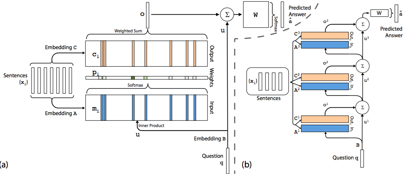
Figure 1: (a) A single-layer version of the considered model. (b) A 3-layer version, obtained via stacking (adopted from [3]).

II-B Variational Bayes in Deep Learning

The main idea of applying variational Bayesian inference to deep learning models consists in calculating a posterior distribution over the network weights given the training data. The benefit of such a learning algorithm setup is that the so-obtained posterior distribution answers predictive queries about unseen data by taking expectations: Prediction is made by averaging the resulting predictions for each possible configuration of the weights, weighted according to their posterior distribution. This allows for accounting for uncertainty, which is prevalent in tasks dealing with sparse training datasets.

Specifically, let us consider a training dataset $\mathcal{D}$. A deep network essentially postulates and fits to the training data a (conditional) likelihood function of the form $p(\mathcal{D}|\boldsymbol{w})$, where $\boldsymbol{w}$ is the vector of network weights. In the case of Bayesian treatments of neural networks, an appropriate prior distribution, $p(\boldsymbol{w})$, is imposed over $\boldsymbol{w}$, and the corresponding posterior is inferred from the data [10]. This consists in introducing an approximate posterior distribution over the network weights, $q(\boldsymbol{w};\boldsymbol{\phi})$, and optimizing it w.r.t. a lower bound to the network log-marginal likelihood $\mathrm{log}\,p(\mathcal{D};\boldsymbol{\phi})$, commonly referred to as the evidence lower bound (ELBO), $\mathcal{L}(\boldsymbol{\phi})$ [26]; it holds

$$\mathrm{log}\,p(\mathcal{D};\boldsymbol{\phi})\geq\mathcal{L}(\boldsymbol{\phi})= \mathbb{E}_{q(\boldsymbol{w};\boldsymbol{\phi})}[\mathrm{log}\,p(\mathcal{D}|\boldsymbol{w})$$ (5)

$$+\mathrm{log}\,p(\boldsymbol{w})-\mathrm{log}\,q(\boldsymbol{w};\boldsymbol{\phi})]$$

where $\mathbb{E}_{q(\boldsymbol{w};\boldsymbol{\phi})}[\cdot]$ is the expectation of a function w.r.t. the random variable $\boldsymbol{w}$, drawn from $q(\boldsymbol{w};\boldsymbol{\phi})$. This is equivalent to minimizing a KL divergence measure between the inferred approximate variational density and the actual underlying distribution.

Turning to the selection of the imposed prior $p(\boldsymbol{w})$, one may opt for a fixed-form isotropic Gaussian:

$$p(\boldsymbol{w})=\mathcal{N}(\boldsymbol{w}|0,\sigma_{0}^{2}\boldsymbol{I})$$ (6)

where $\boldsymbol{I}$ is the identity matrix, and $\mathcal{N}(\cdot|\boldsymbol{\mu},\boldsymbol{\Sigma})$ is a multivariate Gaussian with mean $\boldsymbol{\mu}$ and covariance matrix $\boldsymbol{\Sigma}$. On the other hand, the sought variational posterior $q(\boldsymbol{w};\boldsymbol{\phi})$ is for simplicity and efficiency purposes selected as a diagonal Gaussian of the form:

$$q(\boldsymbol{w};\boldsymbol{\phi})=\mathcal{N}(\boldsymbol{w}|\boldsymbol{\mu},\mathrm{diag}(\boldsymbol{\sigma}^{2}))$$ (7)

where $\boldsymbol{\phi}=\{\boldsymbol{\mu},\boldsymbol{\sigma}^{2}\}$, and $\mathrm{diag}(\boldsymbol{\sigma}^{2})$ is a diagonal matrix with the vector $\boldsymbol{\sigma}^{2}$ on its main diagonal.

An issue with the above formulation is that the entailed posterior expectation $\mathbb{E}_{q(\boldsymbol{w};\boldsymbol{\phi})}[\mathrm{log}\,p(\mathcal{D}|\boldsymbol{w})]$ is analytically intractable; this is due to the non-conjugate nature of deep networks, stemming from the employed nonlinear activation functions. This prohibits taking derivatives of $\mathcal{L}(\boldsymbol{\phi})$ to effect derivation of the sought posterior $q(\boldsymbol{w};\boldsymbol{\phi})$. In addition, approximating this expectation by simply drawing Monte-Carlo (MC) samples from the weights posterior is not an option, due to the prohibitively high variance of the resulting estimator.

To address this issue, one can resort to a simple reparameterization trick: We consider that the MC samples $\boldsymbol{w}^{(s)}$ used to approximate the expectation $\mathbb{E}_{q(\boldsymbol{w};\boldsymbol{\phi})}[\mathrm{log}\,p(\mathcal{D}|\boldsymbol{w})]$ are functions of their posterior mean and variance, as well as a random noise vector, $\boldsymbol{\epsilon}$, sampled from a standard Gaussian distribution [9, 8, 6]. This can be effected by introducing the transform:

$$\boldsymbol{w}=\boldsymbol{\mu}+\boldsymbol{\sigma}\varodot\boldsymbol{\epsilon}$$ (8)

where $\varodot$ denotes the elementwise product of two vectors, and the $\boldsymbol{\epsilon}$ are distributed as $\boldsymbol{\epsilon}\sim\mathcal{N}(\boldsymbol{0},\boldsymbol{I})$. By substituting this transform into the derived ELBO expression, the entailed posterior expectation is expressed as an average over a standard Gaussian density, $p(\boldsymbol{\epsilon})$. This yields an MC estimator with low variance, under some mild conditions [6].

II-C The Student’s-$t$ Distribution

The adoption of the multivariate Student’s-$t$ distribution provides a way to broaden the Gaussian distribution for potential outliers [24, Section 7]. The probability density function (pdf) of a Student’s-$t$ distribution with mean vector $\boldsymbol{\mu}$, covariance matrix $\boldsymbol{\Sigma}$, and $\nu>0$ degrees of freedom is [27]

$$t(\boldsymbol{y}_{t};\boldsymbol{\mu},\boldsymbol{\Sigma},\nu)=\frac{\Gamma\left(\frac{\nu+\delta}{2}\right)|\boldsymbol{\Sigma}|^{-1/2}(\pi\nu)^{-\delta/2}}{\Gamma(\nu/2)\{1+d(\boldsymbol{y}_{t},\boldsymbol{\mu};\boldsymbol{\Sigma})/\nu\}^{(\nu+\delta)/2}}$$ (9)

where $\delta$ is the dimensionality of the observations $\boldsymbol{y}_{t},$ $d(\boldsymbol{y}_{t},\boldsymbol{\mu};\boldsymbol{\Sigma})$ is the squared Mahalanobis distance between $\boldsymbol{y}_{t},\boldsymbol{\mu}$ with covariance matrix $\boldsymbol{\Sigma}$

$$d(\boldsymbol{y}_{t},\boldsymbol{\mu};\boldsymbol{\Sigma})=(\boldsymbol{y}_{t}-\boldsymbol{\mu})^{T}\boldsymbol{\Sigma}^{-1}(\boldsymbol{y}_{t}-\boldsymbol{\mu})$$ (10)

and $\Gamma(s)$ is the Gamma function, $\Gamma(s)=\int_{0}^{\infty}e^{-t}z^{s-1}dz$.

It can be shown (see, e.g., [27]) that, in essence, the Student’s-$t$ distribution corresponds to a Gaussian scale model [28] where the precision scalar is a Gamma distributed latent variable, depending on the degrees of freedom of the Student’s-$t$ density. That is, given

$$\boldsymbol{y}_{t}\sim t(\boldsymbol{\mu},\boldsymbol{\Sigma},\nu)$$ (11)

it equivalently holds that [27]

$$\boldsymbol{y}_{t}|\xi_{t}\sim\mathcal{N}(\boldsymbol{\mu},\boldsymbol{\Sigma}/\xi_{t})$$ (12)

where the precision scalar, $\xi_{t}$, is distributed as

$$\xi_{t}\sim\mathcal{G}\left(\frac{\nu}{2},\frac{\nu}{2}\right)$$ (13)

and $\mathcal{G}(\alpha,\beta)$ is the Gamma distribution.

A graphical illustration of the univariate Student’s-$t$ distribution, with $\boldsymbol{\mu}$, $\boldsymbol{\Sigma}$ fixed, and for various values of the degrees of freedom $\nu$, is provided in Fig. 2. As we observe, as $\nu\rightarrow\infty$, the Student’s-$t$ distribution tends to a Gaussian with the same $\boldsymbol{\mu}$ and $\boldsymbol{\Sigma}$. On the contrary, as $\nu$ tends to zero, the tails of the distribution become longer, thus allowing for a better handling of potential outliers, without affecting the mean or the covariance of the distribution. Thus, by exploiting the heavier tails of the Student’s-$t$ distribution, a probabilistic generative model becomes capable of handling, in a considerably enhanced manner, outliers residing in the fitting datasets. That is, if the modeled phenomenon is actually heavy-tailed, the inferred Student’s-$t$ model will be capable to cope, by yielding a value for the fitted degrees of freedom parameter, $\nu$, e.g., close to 1. On the other hand, if no such heavy-tailed nature does actually characterize the data, the fitted degrees of freedom parameter, $\nu$, will yield a value close to infinity (practically, above 100). In the latter case, the model essentially reduces to a simpler Gaussian density [24, Section 7].

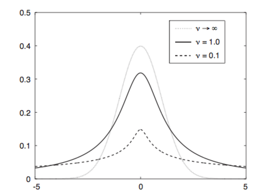
Figure 2: Univariate Student’s-$t$ distribution $t(\boldsymbol{y}_{t};\boldsymbol{\mu},\boldsymbol{\Sigma},\nu)$, with $\boldsymbol{\mu}$, $\boldsymbol{\Sigma}$ fixed, for various values of $\nu$ [29].

II-D The $t$-Divergence

As discussed in Section II.B, conventional variational inference is equivalent to minimization of a KL divergence measure, which is also known as the relative SBG-entropy. Motivated from these facts, and in order to allow for making the most out of the merits (heavy tails) of the $t$-exponential family, the $t$-divergence was introduced in [25] as follows:
Definition 1. The $t$-divergence between two distributions, $q(\boldsymbol{h})$ and $p(\boldsymbol{h})$, is defined as

$$D_{t}(q||p)=\int\tilde{q}(\boldsymbol{h})\mathrm{log}_{t}q(\boldsymbol{h})\mathrm{d}\boldsymbol{h}-\tilde{q}(\boldsymbol{h})\mathrm{log}_{t}p(\boldsymbol{h})\mathrm{d}\boldsymbol{h}$$ (14)

where $\tilde{q}(\boldsymbol{h})$ is called the escort distribution of $q(\boldsymbol{h})$, and is given by

$$\tilde{q}(\boldsymbol{h})=\frac{q(\boldsymbol{h})^{t}}{\int q(\boldsymbol{h})^{t}\mathrm{d}\boldsymbol{h}},\;t\in\mathbb{R}$$ (15)

Importantly, the divergence $D_{t}(q||p)$ preserves the following two properties:

• $D_{t}(q||p)\geq 0,\;\forall q,p$. The equality holds only for $q=p$.

• $D_{t}(q||p)\neq D_{t}(p||q)$.

In the seminal work of [25], it has been shown that by leveraging the above definition of the $t$-divergence, $D_{t}(q||p)$, one can establish an advanced variational inference framework, much more appropriate for modeling data with heavy tails. We exploit these benefits in developing the training and inference algorithms of the proposed $t$-MEM-NN model, as explained in the following Section.

III Proposed Approach

III-A Model Formulation

$t$-MEM-NN extends upon the model design principles discussed previously, by building on the solid theory of variational inference based on the $t$-divergence. It does so by introducing a novel formulation that renders MEM-NN amenable to Bayesian inference.

To effect our modeling goals, we first consider that the postulated embeddings matrices are Student’s-$t$ distributed latent variables. Specifically, let us start by imposing a simple, zero-mean Student’s-$t$ prior distribution over them, with tied degrees of freedom:

$$p(\boldsymbol{A})=t(\mathrm{vec}(\boldsymbol{A})|\boldsymbol{0},\boldsymbol{I},\nu)$$ (16)

$$p(\boldsymbol{B})=t(\mathrm{vec}(\boldsymbol{B})|\boldsymbol{0},\boldsymbol{I},\nu)$$ (17)

$$p(\boldsymbol{C})=t(\mathrm{vec}(\boldsymbol{C})|\boldsymbol{0},\boldsymbol{I},\nu)$$ (18)

where $\mathrm{vec}(\cdot)$ is the matrix vectorization operation, and $\nu>0$ is the degrees of freedom hyperparameter of the imposed priors. On this basis, we seek to devise an efficient means of inferring the corresponding posterior distributions, given the available training data. We postulate that the sought posterior $q(\boldsymbol{A},\boldsymbol{B},\boldsymbol{C};\boldsymbol{\phi})$ factorizes over $\boldsymbol{A}$, $\boldsymbol{B}$, and $\boldsymbol{C}$ (mean-field approximation [19]); the factors are considered to approximately take the form of Student’s-$t$ densities with means, diagonal covariance matrices, and degrees of freedom inferred from the data. Hence, we have:

$$q(\boldsymbol{A};\boldsymbol{\phi})=t(\mathrm{vec}(\boldsymbol{A})|\boldsymbol{\mu}_{\boldsymbol{A}},\mathrm{diag}(\boldsymbol{\sigma}_{\boldsymbol{A}}^{2}),\nu_{\boldsymbol{A}})$$ (19)

$$q(\boldsymbol{B};\boldsymbol{\phi})=t(\mathrm{vec}(\boldsymbol{B})|\boldsymbol{\mu}_{\boldsymbol{B}},\mathrm{diag}(\boldsymbol{\sigma}_{\boldsymbol{B}}^{2}),\nu_{\boldsymbol{B}})$$ (20)

$$q(\boldsymbol{C};\boldsymbol{\phi})=t(\mathrm{vec}(\boldsymbol{C})|\boldsymbol{\mu}_{\boldsymbol{C}},\mathrm{diag}(\boldsymbol{\sigma}_{\boldsymbol{C}}^{2}),\nu_{\boldsymbol{C}})$$ (21)

where $\boldsymbol{\phi}=\{\boldsymbol{\mu}_{i},\boldsymbol{\sigma}_{i}^{2},\nu_{i}\}_{i\in\{\boldsymbol{A},\boldsymbol{B},\boldsymbol{C}\}}$, and $\nu_{i}>0,\forall i$.

On this basis, to perform model training in a way the best exploits the heavy tails of the developed model, we minimize the $t$-divergence between the sought variational posterior and the postulated joint density over the observed data and the model latent variables. Thus, the proposed model training objective becomes

$$q(\boldsymbol{A} ;\boldsymbol{\phi}),q(\boldsymbol{B};\boldsymbol{\phi}),q(\boldsymbol{C};\boldsymbol{\phi}),\boldsymbol{W}$$ (22)

$$= \underset{q,\boldsymbol{W}}{\mathrm{arg\,min}\;}D_{t}\left(q(\boldsymbol{A};\boldsymbol{\phi}),q(\boldsymbol{B};\boldsymbol{\phi}),q(\boldsymbol{C};\boldsymbol{\phi})||p(a;\boldsymbol{A},\boldsymbol{B},\boldsymbol{C},\boldsymbol{W})\right)$$

where $p(a;\boldsymbol{A},\boldsymbol{B},\boldsymbol{C},\boldsymbol{W})=p(a;\boldsymbol{W})p(\boldsymbol{A})p(\boldsymbol{B})p(\boldsymbol{C})$. Then, following the derivations rationale of [25], and by application of simple algebra, the expression of the $t$-divergence in (22) yields

$$D_{t}\big{(}q(\boldsymbol{A};\boldsymbol{\phi}),q(\boldsymbol{B};\boldsymbol{\phi}),q(\boldsymbol{C};\boldsymbol{\phi}) ||p(a;\boldsymbol{A},\boldsymbol{B},\boldsymbol{C},\boldsymbol{W})\big{)}=$$ (23)

$$=D_{t}\left(q(\boldsymbol{A};\boldsymbol{\phi})||p(\boldsymbol{A})\right) +D_{t}\left(q(\boldsymbol{B};\boldsymbol{\phi})||p(\boldsymbol{B})\right)$$

$$+D_{t}\left(q(\boldsymbol{C};\boldsymbol{\phi})||p(\boldsymbol{C})\right) -\mathbb{E}_{\tilde{q}(\cdot;\boldsymbol{\phi})}[\mathrm{log}p(a;\boldsymbol{W})]$$

where $\tilde{q}(\cdot;\boldsymbol{\phi})$ is the escort distribution of the sought variational posterior, and $p(a;\boldsymbol{W})$ is a Multinoulli parameterized via the probability vector $\hat{\boldsymbol{a}}$, given by (4).

Following [25], and based on (16)-(21), we obtain that the $t$-divergence expressions in (23) can be written in the following form:

$$D_{t}\left(q(\boldsymbol{\Theta};\boldsymbol{\phi})||p(\boldsymbol{\Theta})\right)=\sum_{l=1}^{\delta V}\bigg{\{} \frac{\Psi_{ql}}{1-t}\left(1+\frac{1}{\nu_{\boldsymbol{\Theta}}}\right)$$ (24)

$$-\frac{\Psi_{p}}{1-t} \left(1+\frac{[\boldsymbol{\sigma}_{\boldsymbol{\Theta}}^{2}]_{l}+[\boldsymbol{\mu_{\Theta}}]_{l}^{2}}{\nu}\right)\bigg{\}}$$

where $\boldsymbol{\Theta}\in\{\boldsymbol{A},\boldsymbol{B},\boldsymbol{C}\}$, $[\boldsymbol{\xi}]_{l}$ is the $l$th element of a vector $\boldsymbol{\xi}$, we denote

$$\Psi_{ql}\triangleq\left(\frac{\mathrm{\Gamma}(\frac{\nu_{\boldsymbol{\Theta}}+1}{2})}{\mathrm{\Gamma}(\frac{\nu_{\boldsymbol{\Theta}}}{2})(\pi\nu_{\boldsymbol{\Theta}})^{1/2}[\boldsymbol{\sigma}_{\boldsymbol{\Theta}}]_{l}}\right)^{-\frac{2}{\nu_{\boldsymbol{\Theta}}+1}}$$ (25)

$$\Psi_{p}\triangleq\left(\frac{\mathrm{\Gamma}(\frac{\nu+1}{2})}{\mathrm{\Gamma}(\frac{\nu}{2})(\pi\nu)^{1/2}}\right)^{-\frac{2}{\nu+1}}$$ (26)

$\delta$ is the dimensionality of the embeddings, $V$ is the vocabulary size, $\nu$ is the degrees of freedom hyperparameter of the prior, and the free hyperparameter $t$ is set as [25]

$$t=\frac{2}{1+\nu_{\boldsymbol{\Theta}}}+1$$ (27)

III-B Training Algorithm Configuration

As we observe from the preceding discussion, the expectation of the conditional log-likelihood of the model, $\mathbb{E}_{\tilde{q}(\cdot;\boldsymbol{\phi})}[\mathrm{log}p(a;\boldsymbol{W})]$, is computed with respect to the escort distribution of the sought posterior, $\tilde{q}(\cdot;\boldsymbol{\phi})$. Based on (19)-(21), it is easy to show that this escort distribution yields a factorized form, with [25]

$$\tilde{q}(\boldsymbol{\Theta};\boldsymbol{\phi})=t\left(\mathrm{vec}(\boldsymbol{\Theta})|\boldsymbol{\mu_{\Theta}},\frac{\nu_{\boldsymbol{\Theta}}}{\nu_{\boldsymbol{\Theta}}+2}\mathrm{diag}(\boldsymbol{\sigma}_{\boldsymbol{\Theta}}^{2}),\nu_{\boldsymbol{\Theta}}+2\right)$$ (28)

$$\forall\boldsymbol{\Theta}\in\{\boldsymbol{A},\boldsymbol{B},\boldsymbol{C}\}$$

Despite this convenient escort distribution expression, though, this posterior expectation cannot be computed analytically; hence, its gradient becomes intractable. This is due to the nonconjugate nature of $t$-MEM-NN, which stems from its nonlinear assumptions. Apparently, approximating this expectation using a set of $S$ MC samples, $\{\boldsymbol{\Theta}_{s}\}_{s=1}^{S}$, drawn from the escort densities (28), would result in estimators with unacceptably high variance.

In this work, these issues are resolved by adopting the reparameterization trick ideas described in Section II.B, adapted to the $t$-exponential family. Specifically, we perform a smart reparameterization of the MC samples from the Student’s-$t$ escort densities (28) which yields:

$$\boldsymbol{\Theta}_{s}=\boldsymbol{\mu}_{\boldsymbol{\Theta}}+\left(\frac{\nu_{\boldsymbol{\Theta}}}{\nu_{\boldsymbol{\Theta}}+2}\right)^{1/2}\boldsymbol{\sigma}_{\boldsymbol{\Theta}}\boldsymbol{\epsilon}_{s}$$ (29)

where $\boldsymbol{\epsilon}_{s}$ is random Student’s-$t$ noise with unitary variance:

$$\boldsymbol{\epsilon}_{s}\sim t(\boldsymbol{0},\boldsymbol{I},\nu_{\boldsymbol{\Theta}}+2)$$ (30)

Then, the resulting (reparameterized) $t$-divergence objective (23) can be minimized by means of any off-the-shelf stochastic optimization algorithm. For this purpose, in this work we utilize Adagrad; this constitutes a stochastic gradient descent algorithm with adaptive step-size [30], and fast and proven convergence to a local optimum. Adagrad updates the trained posterior hyperparameter set, $\boldsymbol{\phi}$, as well as the output layer weights, $\boldsymbol{W}$, by utilizing the gradient $\triangledown_{\boldsymbol{\phi},\boldsymbol{W}}D_{t}\left(q(\boldsymbol{A};\boldsymbol{\phi}),q(\boldsymbol{B};\boldsymbol{\phi}),q(\boldsymbol{C};\boldsymbol{\phi})||p(a;\boldsymbol{A},\boldsymbol{B},\boldsymbol{C},\boldsymbol{W})\right)$.

On each Adagrad iteration, this gradient is computed using only a small subset (minibatch) of the available training data, as opposed to using the whole training dataset. This allows for computational tractability, no matter what the total number of training examples is. To facilitate convergence, on each algorithm iteration a different minibatch is selected, in a completely random fashion.

In this context, it is important to appropriately select the number of MC samples drawn from (30) during training. In our work, we opt for the computationally efficient solution of drawing just one MC sample during training. One could argue that using only one MC sample is doomed to result in an approximation of limited quality. However, it has been empirically well-established that drawing just one MC sample is sufficient when Adagrad is executed with a small minibatch size compared to the size of the used training dataset [10, 14]. Indeed, this is the case with our experimental evaluations in Section IV. In all cases, network initialization is performed by means of the Glorot uniform scheme, except for the degrees of freedom hyperparameters; these are initialized at high values ($\nu=100$), which essentially reduce the initial Student’s-$t$ densities of our model to simpler Gaussian ones (as discussed in Section II.C) [31].

III-C Inference Procedure

Having obtained a training algorithm for our proposed $t$-MEM-NN model, we can now proceed to elaborate on how inference is performed using our method. As briefly hinted in Section II.B, this consists in drawing a number of MC samples from the inferred posteriors over the model parameters, $q(\cdot;\boldsymbol{\phi}),$ and obtaining the average predictive value of the model that corresponds to these drawn parameter values (samples). According to the related deep learning literature, drawing a set of $S=10$ samples should be enough for inference purposes [10, 14]. We investigate the impact of the number of drawn MC samples to the eventually obtained performance of the inference algorithm of our model in our experiments that follow.

IV Synthetic Question-Answering Tasks

Table I: Considered benchmark dataset: Indicative training data samples from three of the entailed types of tasks.

Sam walks into the kitchen.	Brian is a lion.	Sandra got the milk.
Sam picks up an apple.	Julius is a lion.	Sandra journeyed to the garden.
Sam walks into the bedroom.	Julius is white.	Sandra went back to the bathroom.
Sam drops the apple.	Bernhard is green.	Sandra put down the milk.
Q: Where is the apple?	Q: What color is Brian?	Q: Where was the milk before the bathroom?
A: Bedroom	A: White	A: Garden

Table II: Quantitative assessment: Accuracy results in the test set.

Test Accuracy (%)
	Baseline	$t$-MEM-NN
Task type	MemN2N	1 sample	10 samples
1: 1 supporting fact	100	100	100
2: 2 supporting facts	84	77	84
3: 3 supporting facts	55	55	57
4: 2 argument relations	96	94	96
5: 3 argument relations	88	87	88
6: yes/no questions	92	93	97
7: counting	83	81	85
8: lists/sets	87	87	90
9: simple negation	90	88	92
10: indefinite knowledge	78	81	84
11: basic coreference	85	98	98
12: conjunction	100	100	100
13: compound coreference	89	93	95
14: time reasoning	92	92	96
15: basic deduction	100	100	100
16: basic induction	45	45	46
17: positional reasoning	51	51	53
18: size reasoning	87	89	91
19: path finding	12	12	14
20: agent’s motivation	100	100	100

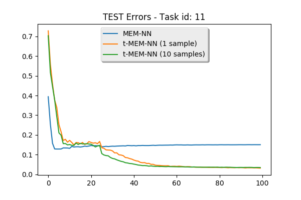
Figure 3: Test error per epoch: Task type #11.

Table III: Attention in task type #1 - story #202.

Facts
1. mary moved to the hallway
1. daniel travelled to the office
2. john went back to the hallway
3. john moved to the office
4. sandra journeyed to the kitchen
5. mary moved to the bedroom

Question

where is daniel?

Answer

office

Supporting Facts

daniel travelled to the office

MemN2N

bedroom

$t$-MEM-NN (1 sample)

bedroom

$t$-MEM-NN (10 samples)

office

(a) Predicted answers.

MemN2N
hop 1	daniel travelled to the office
hop 2	daniel travelled to the office
hop 3	mary moved to the bedroom

$t$-MEM-NN (1 sample)
hop 1	daniel travelled to the office
hop 2	daniel travelled to the office
hop 3	mary moved to the bedroom

$t$-MEM-NN (10 samples)
hop 1	daniel travelled to the office
hop 2	daniel travelled to the office
hop 3	daniel travelled to the office

(b) Model attention per hop.

Table IV: Attention in task type #11 - story #3.

Facts
1. john journeyed to the hallway
2. after that he journeyed to the garden
3. john moved to the office
4. following that he went to the hallway
5. sandra travelled to the bedroom
6. then she moved to the hallway
7. mary travelled to the hallway
8. afterwards she went to the bathroom

Question

where is sandra?

Answer

hallway

Supporting Facts
sandra travelled to the bedroom
then she moved to the hallway

MemN2N

bathroom

$t$-MEM-NN (1 sample)

hallway

$t$-MEM-NN (10 samples)

hallway

(a) Predicted answers.

MemN2N
hop 1	afterwards she went to the bathroom
hop 2	afterwards she went to the bathroom
hop 3	afterwards she went to the bathroom

$t$-MEM-NN (1 sample)
hop 1	sandra travelled to the bedroom
hop 2	then she moved to the hallway
hop 3	then she moved to the hallway

$t$-MEM-NN (10 samples)
hop 1	sandra travelled to the bedroom
hop 2	then she moved to the hallway
hop 3	then she moved to the hallway

(b) Model attention per hop.

Table V: Attention in task type #14 - story #22.

Facts
1. mary went back to the kitchen this morning
2. mary travelled to the school yesterday
3. yesterday fred travelled to the bedroom
4. yesterday bill moved to the park
5. this afternoon bill went back to the park
6. bill went to the school this morning

Question

where was bill before the park?

Answer

school

Supporting Facts
this afternoon bill went back to the park
bill went to the school this morning

MemN2N

park

$t$-MEM-NN (1 sample)

park

$t$-MEM-NN (10 samples)

school

(a) Predicted answers.

MemN2N
hop 1	yesterday bill moved to the park
hop 2	yesterday bill moved to the park
hop 3	yesterday bill moved to the park

$t$-MEM-NN (1 sample)
hop 1	yesterday bill moved to the park
hop 2	this afternoon bill went back to the park
hop 3	yesterday bill moved to the park

$t$-MEM-NN (10 samples)
hop 1	yesterday bill moved to the park
hop 2	this afternoon bill went back to the park
hop 3	bill went to the school this morning

(b) Model attention per hop.

In this Section, we perform a thorough experimental evaluation of our proposed $t$-MEM-NN model. We provide a quantitative assessment of the efficacy, the effectiveness, and the computational efficiency of our approach, combined with deep qualitative insights into few of its key performance characteristics. To this end, we utilize a publicly available benchmark, which is popular in the recent literature, namely the set of synthetic question-answering (QA) tasks defined in [32] (bAbI). Specifically, we consider the English-Language tasks of the bAbI dataset that comprise 1K training examples (en-1K tasks). This dataset comprises 20 different types of tasks, which are characterized by different qualitative properties. Some of them are harder to be learned, while some others are much easier.

The idea of all the types of tasks entailed in this dataset is rather simple. Each task consists of a set of statements (facts), a question, and an answer. The answer comprises only one word from the available vocabulary. Given the facts, a question is asked and an answer is expected. Then, model performance can be evaluated on the basis of the percentage of generated answers that match the available groundtruth. To allow for a better feeling of what our dataset looks like, we provide indicative samples from three of the entailed types of tasks in Table I. Note that the available dataset also provides additional supporting facts that may be made use of by the trained models.

To provide some comparative results, we evaluate two variants of our method, namely one where inference is performed using only a single MC sample (drawn from the model posteriors), and another one where 10 MC samples are used. In all cases, training is performed by drawing just one MC sample. In addition, we compare to the state-of-the-art alternative that is the closest related to our approach, namely the MemN2N method of [3]. Our source codes have been developed in Python, using the TensorFlow library [33], as well as open-source software published by Dominique Luna. Our experiments are run on an Intel Xeon server with 64GB RAM and an NVIDIA Tesla K40 GPU.

IV-A Experimental Setup

Model training is performed by utilizing the training dataset provided in the used en-1K bAbI benchmark. This comprises 1000 examples from each type of task; from these, we randomly select 900 samples to perform training, and retain the remainder 100 for validation purposes. Each training example comprises the full set of data pertaining to the task, including the correct answer (which we expect the system to generate), apart from the corresponding question and available statements (facts). On this basis, a trained model is evaluated by presenting it with the facts and the questions pertaining to each example in the test set, and running its inference algorithm to obtain a predicted answer. The available test set comprises 1000 cases from each task type, which are completely unknown to the trained models.

Since the used benchmark comprises a multitude of task types, we train a different model (of each evaluated method) for each task type. An obvious advantage of such a modeling setup consists in the fact that it allows for the trained models to be finely-tuned to data with very specific patterns. On the other hand, the imposed weight tying across model layers is a strong safeguard against possible model overfitting.

Turning to the selection of the hyperparameters of the training algorithms, we emphasize that we adopt exactly the same configuration for both our model and the baseline. Specifically, we perform training for 100 epochs, as also suggested in [3]. Adagrad is carried out by splitting our training data into 32 minibatches. The learning rate is initialized at $\eta=0.01$, and is annealed every 25 epochs by $\eta/2$, until the maximum number of epochs is reached (similar to [3]). Glorot initialization for all trained models is performed via a Gaussian distribution with zero mean and $\sigma=0.1$. The postulated models employ an external memory size of 50 sentences. Nil words are padded with zero embedding (zero one-hot encodings). The embedding space size, $\delta$, is set to 20; this is shown in [3] to work best for the MemN2N model. In order to calculate the output (predicted answer) for each problem, 3 computational steps (hops) are performed, similar to the suggestions of [3].

IV-B Quantitative Assessment

In this Section, the accuracy of the model-generated predictions is measured and reported. In order for a trained model to be considered successful in some type of task, we stipulate that a 95% accuracy must be reached, similar to [3]. The test-set accuracy results obtained under our prescribed experimental setup are provided in Table II. Expectably, increasing the number of MC samples drawn to perform inference improves performance in the most challenging of the task types, while retaining performance in the rest. As we observe, our approach manages to pass our set success threshold of 95% accuracy in 9 task types (# 1, 4, 6, 11, 12, 13, 14, 15, 20), thus outperforming the MemN2N baseline which passes the threshold in only 5 cases (# 1, 4, 12, 15, 20). Another characteristic finding is that our approach outperforms the baseline in most tasks, and achieves the same performance in the few rest. In our perception, this finding vouches for the better capacity of our approach to learn the underlying distributions in the modeled dataset. Of course, one also observes that our method does not offer significant improvements on the types of tasks for which the baseline has low accuracy. However, this apparently constitutes an inherent weakness of the whole learning paradigm adopted by MEM-NN networks; this cannot be rectified by introducing better inference mechanisms, as we do in this work.

Further, to show how the test error of the considered approaches converges over the training algorithm epochs, in Fig. 3 we depict the evolution of the test error for an indicative task type, in one execution of our experiments. We observe that both variants of our approach (i.e., using one or ten MC samples for performing inference) converge gradually and consistently over the training algorithm epochs. In contrast, the baseline MemN2N approach appears to reach its best performance early-on during training, and subsequently remains almost stable.

IV-C Qualitative Assessment

To provide some qualitative insights into the inferred question-answering rationale of our approach, and how this compares to the original MemN2N, in Tables III - V we illustrate what the inferred attention vectors look like in three indicative test cases. More specifically, we record which fact each model mostly focuses its attention on, on every hop; further, we compare this result to the supporting facts included in the dataset. Our so-obtained results indicate that the proposed approach manages to better focus on the most salient information (sentences), as indicated by the provided supporting facts. This outcome offers a strong intuitive explanation of the reasons why $t$-MEM-NN appears to outperform the baseline, in most of the considered task types.

IV-D Computational Times

Apart from inferential accuracy, the computational costs of a devised method constitute another aspect which affects its efficacy. To allow for objectively examining this aspect, we have developed all the evaluated algorithms using the same software platform, and executed them on the same machine (each time without concurrently running any other user application). Then, we recorded the resulting wall-clock times, for both model training and inference.

As we have observed, baseline MemN2N training requires an average of 146.5 msec per minibatch, while our approach imposes a negligible increase, requiring an average of 149.8 msec. This is reasonable, since training of our model entails the same set of computations as baseline MemN2N, with the only exception being the computation of the $t$-divergence terms pertaining to the degrees of freedom parameters, which are of linear complexity. Thus the observed slight increase in computational times, which is clearly worth it for the improved model performance.

Turning to the computational costs of the inference algorithm, we observe that our approach requires computational times comparable to MemN2N in order to generate one answer. This is clearly reasonable, since both models entail the same set of feedforward computations. On the other hand, it is significant to underline that the extra computational costs of $t$-MEM-NN that arise from an increase in the number of MC samples drawn to perform inference (from just one to ten) are completely negligible. Indeed, an average increase of 0.1 msec was observed. This was well-expected, since the extra matrix multiplications that arise from the use of multiple drawn MC samples are completely parallelizable over commercially available, modern GPU hardware.

IV-E Computational Complexity

Let us denote as $n$ the dimensionality of the model input. In essence, this corresponds to the size of the used dictionary, $V$, as discussed in Section II.A. In both the cases of the MemN2N and $t$-MEM-NN models, forward propagation is dominated by the same type of matrix multiplications. In the case of MemN2N, these are effected by making use of the model parameter estimators, $\boldsymbol{\Theta}$; in the case of the $t$-MEM-NN counterpart, we use samples of these parameters drawn by making use of their corresponding means, $\boldsymbol{\mu}_{\boldsymbol{\Theta}}$, diagonal covariances, $\boldsymbol{\sigma}_{\boldsymbol{\Theta}}^{2}$ , and degrees of freedom, $\nu_{\boldsymbol{\Theta}}$. On the other hand, based on our model description provided in Section II.A, a MemN2N or $t$-MEM-NN model comprising $k$ hops in memory comprises $2k+1$ layers. Then, following [34], and considering that each model layer may comprise $n$ output units at most (in which case it extracts overcomplete representations), the run-time complexity of the model inference algorithm (forward propagation) becomes $\mathcal{O}(n^{3}(2k+1))=\mathcal{O}(n^{3})$. This is common for the MemN2N and $t$-MEM-NN models.

Studying the case of backprop training of the MemN2N and $t$-MEM-NN models is more involved. Specifically, by examining Eq. (24) we observe that the objective function involved in $t$-MEM-NN model training entails one extra operation compared to the simple categorical cross-entropy of the MemN2N model; this is the set of $\Gamma(\cdot)$ functions, computed over all the degrees of freedom parameters, $\nu_{\boldsymbol{\Theta}}$. Our computation of the $\Gamma(\cdot)$ function is based on the Lanczos approximation [35]; this essentially reduces to a simple vector inner product and some additional elementary computations. Similarly we approximate its derivative, widely known as the Digamma function. Thus, the dominant source of computationl costs of model training, for both models, are identical. Considering for simplicity that the total number of training algorithm iterations is $\mathcal{O}(n)$, this yields a computational complexity of $\mathcal{O}(n^{5}(2k+1))=\mathcal{O}(n^{5})$ for both MemN2N and $t$-MEM-NN [34].

IV-F Further Insights

IV-F1 Effect of the number of hops

In the previous experimental evaluations, we performed three memory hops, following the suggestions of [3]. Yet, it is desirable to know how $t$-MEM-NN performance may be affected if we change this number. To get a proper answer to this question, we repeat our experiments considering only one memory hop, as well as an increased number of five hops. We provide the so-obtained results in Tables VI and VII. As we observe, conducting only one hop in memory results in a significant performance impairment in the vast majority of the considered task types. This way, our model manages to pass the success threshold in only two of the considered task types (#1 and 12), as opposed to the eight task types attained when performing three memory hops. On the other hand, a further increase of the number of hops from three to five seems to undermine the obtained performance. Indeed, $t$-MEM-NN passes the success threshold in only six task types, namely task types #1, 4, 11, 12, 15, 20. We posit that these outcomes are due to the structure of the used dataset, as it also becomes obvious from the number of available supporting facts, which is more than one in most cases, but it seldom exceeds three.

Table VI: $t$-MEM-NN accuracy in the test set, performing just one memory hop.

Test Accuracy (%)
Task type	1 sample	10 samples
1: 1 supporting fact	100	100
2: 2 supporting facts	34	35
3: 3 supporting facts	23	23
4: 2 argument relations	79	80
5: 3 argument relations	87	87
6: yes/no questions	69	69
7: counting	52	56
8: lists/sets	33	35
9: simple negation	77	80
10: indefinite knowledge	44	47
11: basic coreference	25	28
12: conjunction	96	99
13: compound coreference	92	93
14: time reasoning	21	23
15: basic deduction	57	75
16: basic induction	44	46
17: positional reasoning	48	48
18: size reasoning	85	86
19: path finding	9	9
20: agent’s motivation	83	84

Table VII: $t$-MEM-NN accuracy in the test set, increasing the number of memory hops to five.

Test Accuracy (%)
Task type	1 sample	10 samples
1: 1 supporting fact	100	100
2: 2 supporting facts	78	82
3: 3 supporting facts	56	57
4: 2 argument relations	93	96
5: 3 argument relations	87	87
6: yes/no questions	73	78
7: counting	78	81
8: lists/sets	87	89
9: simple negation	83	86
10: indefinite knowledge	82	84
11: basic coreference	96	97
12: conjunction	98	99
13: compound coreference	90	90
14: time reasoning	87	89
15: basic deduction	94	96
16: basic induction	44	46
17: positional reasoning	50	51
18: size reasoning	89	90
19: path finding	11	14
20: agent’s motivation	100	100

Table VIII: $t$-MEM-NN accuracy in the test set, reducing the embedding size to $\delta=10$.

Test Accuracy (%)
Task type	1 sample	10 samples
1: 1 supporting fact	100	100
2: 2 supporting facts	55	56
3: 3 supporting facts	31	34
4: 2 argument relations	79	81
5: 3 argument relations	83	83
6: yes/no questions	60	61
7: counting	77	77
8: lists/sets	85	85
9: simple negation	70	70
10: indefinite knowledge	71	75
11: basic coreference	96	97
12: conjunction	98	98
13: compound coreference	92	92
14: time reasoning	83	83
15: basic deduction	70	74
16: basic induction	45	45
17: positional reasoning	50	50
18: size reasoning	87	87
19: path finding	10	10
20: agent’s motivation	100	100

Table IX: $t$-MEM-NN accuracy in the test set, increasing the embedding size to $\delta=50$.

Test Accuracy (%)
Task type	1 sample	10 samples
1: 1 supporting fact	100	100
2: 2 supporting facts	73	78
3: 3 supporting facts	52	55
4: 2 argument relations	90	91
5: 3 argument relations	85	86
6: yes/no questions	72	78
7: counting	79	81
8: lists/sets	86	89
9: simple negation	86	87
10: indefinite knowledge	80	82
11: basic coreference	95	96
12: conjunction	99	99
13: compound coreference	93	95
14: time reasoning	81	84
15: basic deduction	98	100
16: basic induction	44	45
17: positional reasoning	50	52
18: size reasoning	89	91
19: path finding	11	13
20: agent’s motivation	100	100

IV-F2 Altering the embedding space dimensionality

In addition, it is interesting to examine what the effect of the embedding space dimensionality is on the performance of our approach. Indeed, it is reasonable to expect that the larger the embedding space the more potent a postulated model is. However, the entailed increase in the trainable model parameters does also come at the cost of considerably higher overfitting tendencies. These might eventually undermine the obtained accuracy profile of $t$-MEM-NN.

To examine these aspects, we repeat our experiments considering a smaller embeddings size than the one suggested in [3], specifically $\delta=10$, as well as a much larger one, specifically $\delta=50$. The outcomes of this investigation are depicted in Tables VIII and IX, respectively. As we observe, decreasing the postulated embedding space dimensionality to $\delta=10$ results in worse model performance, since the model passes the success threshold in only four task types (#1, 11, 12, 20). Similarly interesting are the findings pertaining to an increase of the embedding space size to $\delta=50$. In this case, average model performance over all the considered task types remains essentially stable. Thus, it seems that model performance reaches a plateau as we continue to increase the size of the embeddings. Note also that postulating either $\delta=10$ or $\delta=50$ results in $t$-MEM-NN passing the success threshold in exactly the same set of task types as when we postulate $\delta=20$.

To summarize, increasing the embedding space size does not appear to be worth the extra computational costs. Indeed, $t$-MEM-NN requires an extra 2.2 msec to generate one answer when $\delta$ increases from 20 to 50, which represents an average increase by 62%. On the other hand, predictive accuracy does not yield any considerable increase.

IV-F3 Joint task modeling

In all the previous experiments, we have trained a distinct model on each one of the 20 types of QA tasks included in the considered en-1K bAbI benchmark. However, one could also consider jointly training one single model on data from all the included task types. Clearly, one may argue that this alternative approach might make it more difficult for the trained model to distinguish between fine patterns. However, it is also the case that, by training a joint model on all task types, we also allow for a significantly reduced overfitting tendency (by increasing the effective number of training data). Hence, we consider training a single model on all the task types; we train for 60 epochs, and anneal the learning rate every 15 epochs.

Our results, obtained by setting the latent space dimensionality equal to $\delta=20$, and by employing 3 memory hops, are depicted in Table X. It is evident that, similar to the single-task setup, inference using 10 MC samples yields better average performance than using just one. Considering the set success threshold of 95% accuracy, we obtain that our method succeeds in 9 task types (# 1, 6, 9, 10, 12, 13, 14, 15, 20); this way, it outperforms baseline MemN2N by one task. Note also that $t$-MEM-NN performance is greater than MemN2N in all these tasks.

Table X: Joint-modeling setup: Accuracy results in the test set.

Test Accuracy (%)
	Baseline	$t$-MEM-NN
Task type	MemN2N	1 sample	10 samples
1: 1 supporting fact	99	100	100
2: 1 supporting facts	86	61	79
3: 3 supporting facts	71	45	60
4: 2 argument relations	85	77	85
5: 3 argument relations	86	82	86
6: yes/no questions	96	99	100
7: counting	84	84	85
8: lists/sets	89	88	89
9: simple negation	96	99	99
10: indefinite knowledge	92	91	95
11: basic coreference	94	90	91
12: conjunction	98	99	100
13: compound coreference	97	93	98
14: time reasoning	88	91	96
15: basic deduction	98	97	100
16: basic induction	46	46	48
17: positional reasoning	55	55	58
18: size reasoning	59	67	71
19: path finding	10	14	17
20: agent’s motivation	100	100	100

IV-F4 Experimental evaluation with the rest of the available tasks

Further, for completeness sake, we examine how the performance of our model compares to the competition when it comes to considering the rest of the tasks available in the bAbI dataset. That is, we report results on the 20 QA tasks that are developed in the Hindi language, that comprise both 1K as well as 10K training examples, or employ random shuffling. These are denoted as en-10K, hn-1K, hn-10K, shuffle-1K, and shuffle-10K, respectively. Our findings, obtained by setting the latent space dimensionality equal to $\delta=20$, and by employing 3 memory hops, are depicted in Tables XI-XV. As we observe, in all cases our approach exceeds the 95% success threshold in more tasks than the baseline. This is yet another result that vouches for the validity of our theoretical claims, and the efficacy of our algorithmic construction and derivations.

Table XI: Accuracy results in the Hindi/1k test set.

Test Accuracy (%)
	Baseline	$t$-MEM-NN
Task type	MemN2N	1 sample	10 samples
1: 1 supporting fact	99	100	100
2: 1 supporting facts	85	85	88
3: 3 supporting facts	53	50	55
4: 2 argument relations	97	96	98
5: 3 argument relations	88	85	89
6: yes/no questions	89	89	89
7: counting	83	83	84
8: lists/sets	88	87	90
9: simple negation	89	89	92
10: indefinite knowledge	78	75	82
11: basic coreference	84	90	98
12: conjunction	99	99	99
13: compound coreference	89	93	95
14: time reasoning	93	92	96
15: basic deduction	100	98	100
16: basic induction	45	45	47
17: positional reasoning	49	45	51
18: size reasoning	86	86	93
19: path finding	13	12	13
20: agent’s motivation	100	100	100

Table XII: Accuracy results in the Shuffled/1k test set.

Test Accuracy (%)
	Baseline	$t$-MEM-NN
Task type	MemN2N	1 sample	10 samples
1: 1 supporting fact	100	100	100
2: 1 supporting facts	79	75	79
3: 3 supporting facts	49	50	54
4: 2 argument relations	95	93	95
5: 3 argument relations	86	85	86
6: yes/no questions	91	90	94
7: counting	80	80	84
8: lists/sets	87	87	89
9: simple negation	89	89	94
10: indefinite knowledge	79	80	83
11: basic coreference	83	92	100
12: conjunction	99	99	100
13: compound coreference	89	90	95
14: time reasoning	91	91	96
15: basic deduction	100	99	100
16: basic induction	45	45	46
17: positional reasoning	50	49	52
18: size reasoning	86	88	91
19: path finding	12	12	13
20: agent’s motivation	100	100	100

Table XIII: Accuracy results in the en/10k test set.

Test Accuracy (%)
	Baseline	$t$-MEM-NN
Task type	MemN2N	1 sample	10 samples
1: 1 supporting fact	100	100	100
2: 1 supporting facts	98	97	100
3: 3 supporting facts	83	85	89
4: 2 argument relations	100	98	100
5: 3 argument relations	99	99	99
6: yes/no questions	100	99	100
7: counting	95	95	97
8: lists/sets	97	98	100
9: simple negation	99	98	99
10: indefinite knowledge	96	96	99
11: basic coreference	91	94	100
12: conjunction	100	100	100
13: compound coreference	94	94	98
14: time reasoning	97	95	100
15: basic deduction	100	100	100
16: basic induction	47	47	47
17: positional reasoning	57	57	57
18: size reasoning	89	88	92
19: path finding	33	33	36
20: agent’s motivation	100	100	100

Table XIV: Accuracy results in the Hindi/10k test set.

Test Accuracy (%)
	Baseline	$t$-MEM-NN
Task type	MemN2N	1 sample	10 samples
1: 1 supporting fact	100	100	100
2: 1 supporting facts	97	97	100
3: 3 supporting facts	83	81	91
4: 2 argument relations	99	99	99
5: 3 argument relations	98	98	99
6: yes/no questions	100	100	100
7: counting	94	93	97
8: lists/sets	97	97	99
9: simple negation	98	98	99
10: indefinite knowledge	93	93	97
11: basic coreference	94	96	100
12: conjunction	100	100	100
13: compound coreference	96	97	100
14: time reasoning	98	98	100
15: basic deduction	100	100	100
16: basic induction	46	43	47
17: positional reasoning	56	56	57
18: size reasoning	91	91	94
19: path finding	31	32	35
20: agent’s motivation	100	100	100

Table XV: Accuracy results in the Shuffled/10k test set.

Test Accuracy (%)
	Baseline	$t$-MEM-NN
Task type	MemN2N	1 sample	10 samples
1: 1 supporting fact	100	100	100
2: 1 supporting facts	97	98	100
3: 3 supporting facts	83	83	88
4: 2 argument relations	100	100	100
5: 3 argument relations	99	98	99
6: yes/no questions	100	100	100
7: counting	95	95	97
8: lists/sets	96	96	99
9: simple negation	99	99	100
10: indefinite knowledge	97	97	99
11: basic coreference	92	94	100
12: conjunction	100	100	100
13: compound coreference	96	96	100
14: time reasoning	98	95	100
15: basic deduction	100	100	100
16: basic induction	47	47	48
17: positional reasoning	56	56	57
18: size reasoning	90	90	92
19: path finding	35	35	38
20: agent’s motivation	100	100	100

IV-F5 Do we actually need to infer heavy-tailed posteriors?

As we have already discussed, the central assumption in the formulation of our model that the imposed posteriors are of multivariate Student’s-$t$ form allows to account for heavy-tailed underlying densities, with power-law nature. However, a question that naturally arises is whether this assumption actually addresses an existing problem. That is, whether the underlying densities are actually heavy-tailed. To address this question, we can leverage some attractive properties of the Student’s-$t$ distribution. Specifically, as we have explained in Section II.C, the degrees of freedom parameter of a Student’s-$t$ density controls how heavy its tails are. This way, a model employing Student’s-$t$ densities effectively modifies, through model fitting, how heavy its tails are, to account for the actual needs of the application at hand.

Therefore, examining the degrees of freedom values of the fitted model posteriors is a natural means of deducing whether the imposition of Student’s-$t$ densities is actually worthwhile, or a simpler Gaussian assumption would suffice. Our findings can be summarized as follows: In all the experimental cases reported above, the posteriors over the input embedding matrices $\boldsymbol{A}$ and $\boldsymbol{B}$, given in (19) and (20), yield values $\nu_{\boldsymbol{A}},\nu_{\boldsymbol{B}}\leq 5$, while for the output embeddings $\boldsymbol{C}$, given by (21), we have $\nu_{\boldsymbol{C}}\leq 20$. These findings imply that all our fitted models end up requiring degrees of freedom parameter values low enough to account for quite heavy tails. Thus, our empirical experimental findings vouch for the efficacy of our assumptions.

V Guess the Number

We conclude our experimental investigations by considering a setup that allows for us to evaluate whether our model is capable of learning latent abstract concepts by engaging in conversation with a teacher. Specifically, our devised experimental setup emulates a kid’s game named “Guess the number.” This well-known game is played by two entities, the teacher and the student; on each round, the teacher picks an integer number between given boundaries, and the student tries to guess which number the teacher has originally selected. When the student guesses a number different than the target, the teacher provides them a hint whether the guessed number is greater or less than it. On the sequel, the student has to make another guess, following the limits dictated in the preceding conversation (i.e., all previous guesses and provided hints). The game continues until either the student guesses the target number or we reach the maximum allowed numbers of tries.

Under this experimental rationale, we have constructed datasets that correspond to two different scenarios; in these, the chosen numbers lie between: (a) 0 and 10; and (b) 0 and 100. The maximum number of tries is set to 100 for both scenarios. In addition, we perform evaluation with a diverse number of training examples including 100, 1K, and 10K, in order to assess the effect of the training dataset size. The latent space dimensionality of all the evaluated models is set equal to $\delta=20$, while we employ 3 memory hops, similar to Section IV.B. Model evaluation is performed on 100 distinct test games, in all cases. Inference for $t$-MEM-NN is run with the number of drawn MC samples set to 1 or 10; training is performed by drawing just one MC sample.

For the purpose of quantitative performance evaluation of the trained models, we have defined and use three metrics: (i) accuracy, which describes the average percentage of correct decisions; a guess is considered correct when the guessed number is within the limits defined by the conversation’s history; (ii) success, which describes the average percentage of games where the target number was correctly guessed within the preset limit of 100 tries; and (iii) rounds, the average number of guesses made before the target was found. The last metric obviously concerns only successful games.

Our so-obtained results are depicted in Tables XVI and XVII. To allow for the reader to get an insight into the construction of the considered game, as well as the generated outputs of MemN2N and our proposed approach, we provide two characteristic output samples of the evaluated models in Table XVIII. According to the outcome of this assessment, it is obvious that our proposed approach outperforms the baseline model in all metrics for all scenarios.

Table XVI: Guess the number: selected numbers take values between 0 and 10.

100 Training examples
	Baseline	$t$-MEM-NN	$t$-MEM-NN
Metric	MemN2N	1 sample	10 samples
Accuracy (%)	77	87	91
Success (%)	86	95	98
Rounds	4.3	3.9	3.6

1k Training examples
	Baseline	$t$-MEM-NN	$t$-MEM-NN
Metric	MemN2N	1 sample	10 samples
Accuracy (%)	99	100	100
Success (%)	100	100	100
Rounds	4.2	3.8	3.6

10k Training examples
	Baseline	$t$-MEM-NN	$t$-MEM-NN
Metric	MemN2N	1 sample	10 samples
Accuracy (%)	97	99	100
Success (%)	98	100	100
Rounds	4.0	3.8	3.7

Table XVII: Guess the number: selected numbers take values between 0 and 100.

100 Training examples
	Baseline	$t$-MEM-NN	$t$-MEM-NN
Metric	MemN2N	1 sample	10 samples
Accuracy (%)	17	19	21
Success (%)	20	28	31
Rounds	7.7	5.1	3.2

1k Training examples
	Baseline	$t$-MEM-NN	$t$-MEM-NN
Metric	MemN2N	1 sample	10 samples
Accuracy (%)	30	49	55
Success (%)	45	61	72
Rounds	8.7	8.2	7.7

10k Training examples
	Baseline	$t$-MEM-NN	$t$-MEM-NN
Metric	MemN2N	1 sample	10 samples
Accuracy (%)	63	78	85
Success (%)	68	89	97
Rounds	12.6	9.1	8.5

Table XVIII: $t$-MEM-NN: Sample output of “Guess the number” game.

——————————-

Model: t-MEM-NN

min: 0

max: 100

Train examples: 1000

——————————-

——————————-

**** TESTING MODEL STARTS ****

——————————-

Select a number between 0 and 100

Round: 1

————-

Selection: 76

Correct: Selection within Bounds!

Accuracy: = 1.0

min_num: -1

max_num: 101

Hint: Target is a smaller number

Round: 2

————-

Selection: 100

Wrong: Selection Out of Bounds!

Accuracy: = 0.5

min_num: -1

max_num: 76

Hint: Target is a smaller number

Round: 3

————-

Selection: 1

Correct: Selection within Bounds!

Accuracy: = 0. 66

min_num: -1

max_num: 76

Hint: Target is a larger number

Round: 4

————-

Selection: 59

Correct: Selection within Bounds!

Accuracy: = 0.75

min_num: 1

max_num: 76

Hint: Target is a smaller number

Round: 5

————-

Selection: 11

Correct: Selection within Bounds!

Accuracy: = 0.8

min_num: 1

max_num: 59

Hint: Target is a larger number

Round: 6

————-

Selection: 56

Correct: Selection within Bounds!

Accuracy: = 0.83

min_num: 11

max_num: 59

Hint: Target is a larger number

Round: 7

————-

Selection: 54

Wrong: Selection Out of Bounds!

Accuracy: = 0.71

min_num: 56

max_num: 59

Hint: Target is a larger number

Round: 8

————-

Selection: 57

Correct: Selection within Bounds!

Accuracy: = 0.75

min_num: 56

max_num: 59

*************************************************

Congratulations, the target is 57

You found the correct answer after 8 rounds

Accuracy: 0.75

VI Conclusions

In this paper, we attacked the problem of modeling long-term dependencies in sequential data. Specifically, we focused on question-answering bots; these inherently require the ability to perform multiple computational steps of analyzing observed patterns over long temporal horizons, and on multiple time-scales. To achieve this goal, one may resort to the paradigm of neural attention models that operate over large external memory modules. This is a recent development in the field of machine learning, yielding state-of-the-art performance in challenging benchmark tasks.

In this context, the core contribution of our work was the provision of a novel inferential framework for this class of models, which allows to account for the uncertainty in the modeled data. This is a significant issue when dealing with sparse datasets, which are prevalent in real-world the considered tasks. In addition, our method was carefully crafted so as to best accommodate data with heavy-tailed distributions, which are typical in multivariate sequences.

To achieve these goals, we devised a novel Bayesian inference-driven algorithmic formulation of end-to-end-trainable MEM-NNs. Specifically, we considered a stochastic model formulation, where the trainable parameters (embedding matrices) of the network are imposed appropriate prior distributions, and corresponding posteriors are inferred by means of variational Bayes. To allow for accommodating heavy-tailed data, we postulated latent variables belonging to the $t$-exponential family; specifically, we considered multivariate Student’s-$t$ densities. In the same vein, and in order to allow for reaping the most out of the data modeling power of Student’s-$t$ densities, we performed variational inference for our model under a novel objective function construction. This was based on a $t$-divergence criterion, which offers an attractive alternative to the KL divergence (that is minimized in conventional variational Bayes), tailored to heavy-tailed data.

We performed an extensive experimental evaluation of our approach using challenging question-answering benchmarks. We provided thorough insights into the inferential outcomes of our approach, and how these compare to the competition. We also illustrated that our proposed approach achieves the reported accuracy improvement without undermining computational efficiency, both in training time and in prediction generation time.

One research direction that we have not considered in this work concerns the possibility of imposing nonelliptical or skewed distributions on the postulated latent variables. Indeed, many researchers in the past have shown that conventional generative models for sequential data, e.g. hidden Markov models, can yield significant benefits by considering nonelliptically contoured latent state densities, such as the multivariate normal inverse Gaussian (MNIG) distribution [36]. On the other hand, the efficacy and the potential advantages of introducing skewed latent variable assumptions in the context of DL models was empirically demonstrated in [14]. Nevertheless, such assumptions certainly come at the cost of increased computational complexity. Hence, we reckon that progressing beyond the elliptical class of distributions for formulating the assumptions of our model is a worthwhile future research direction. It might allow for even higher modeling performance, but requires novel theoretical developments to ensure retainment of the method’s computational efficiency. Thus, these opportunities remain to be explored in our future research.

References

- [1] A. Graves, G. Wayne, and I. Danihelka, “Neural Turing machines,” in Proc. NIPS, 2014.
- [2] J. Weston, S. Chopra, and A. Bordes, “Memory networks,” in Proc. ICLR, 2015.
- [3] S. Sukhbaatar, A. Szlam, J. Weston, and R. Fergus, “End-to-end memory networks,” in Proc. NIPS, 2015.
- [4] A. Rush, S. Chopra, and J. Weston, “A neural attention model for abstractive sentence summarization,” in Proc. ACL, 2015.
- [5] G. K. Zipf, The psychology of language. Houghton-Mifflin, 1935.
- [6] D. Kingma and M. Welling, “Auto-encoding variational Bayes,” in Proc. ICLR’14, 2014.
- [7] D. P. Kingma, D. J. Rezende, S. Mohamed, and M. Welling, “Semi-supervised learning with deep generative models,” in Proc. NIPS’14, 2014.
- [8] D. J. Rezende, S. Mohamed, and D. Wierstra, “Stochastic backpropagation and approximate inference in deep generative models,” in Proc. ICML, 2014.
- [9] D. J. Rezende and S. Mohamed, “Variational inference with normalizing flows,” in Proc. ICML, 2015.
- [10] C. Blundell, J. Cornebise, K. Kavukcuoglu, and D. Wierstra, “Weight uncertainty in neural networks,” in Proc. ICML, 2015.
- [11] M. Jordan, Z. Ghahramani, T. Jaakkola, and L. Saul, “An introduction to variational methods for graphical models,” in Learning in Graphical Models, M. Jordan, Ed. Dordrecht: Kluwer, 1998, pp. 105–162.
- [12] M. J. Wainwright and M. I. Jordan, “Graphical models, exponential families, and variational inference,” Foundations and Trends in Machine Learning, vol. 1, no. 1-2, pp. 1–305, 2008.
- [13] A. Kosinski, “A procedure for the detection of multivariate outliers,” Computational Statistics and Data Analysis, vol. 29, pp. 145–161, 1999.
- [14] H. Partaourides and S. P. Chatzis, “Asymmetric deep generative models,” Neurocomputing, vol. 241, pp. 90–96, 2017.
- [15] C. Tsallis, “Possible generalization of Boltzmann-Gibbs statistics,” J. Stat. Phys., vol. 52, pp. 479–487, 1998.
- [16] A. Sousa and C. Tsallis, “Student’s - and -distributions: Unified derivation from an entropic variational principle,” Physica A, vol. 236, pp. 52–57, 1994.
- [17] C. Tsallis, R. S. Mendes, and A. R. Plastino, “The role of constraints within generalized nonextensive statistics.” Physica A, vol. 261, pp. 534–554, 1998.
- [18] J. Naudts, “Deformed exponentials and logarithms in generalized thermostatistics,” Physica A, vol. 316, pp. 323– 334, 2002.
- [19] ——, “Generalized thermostatistics and mean-field theory,” Physica A, vol. 332, pp. 279–300, 2004.
- [20] ——, “Estimators, escort proabilities, and -exponential families in statistical physics,” Journal of Inequalities in Pure and Applied Mathematics, vol. 5, no. 4, 2004.
- [21] S. P. Chatzis and D. Kosmopoulos, “A Variational Bayesian Methodology for Hidden Markov Models utilizing Student’s-t Mixtures,” Pattern Recognition, vol. 44, no. 2, pp. 295–306, Feb. 2011.
- [22] S. Chatzis, D. Kosmopoulos, and T. Varvarigou, “Signal modeling and classification using a robust latent space model based on distributions,” IEEE Trans. Signal Processing, vol. 56, no. 3, March 2008.
- [23] ——, “Robust sequential data modeling using an outlier tolerant hidden Markov model,” IEEE Trans. Pattern Analysis and Machine Intelligence, vol. 31, no. 9, pp. 1657–1669, 2009.
- [24] G. McLachlan and D. Peel, Finite Mixture Models. New York: Wiley Series in Probability and Statistics, 2000.
- [25] N. Ding, S. N. Vishwanathan, and Y. Qi, “-divergence based approximate inference,” in Proc. NIPS, 2011.
- [26] H. Attias, “A variational Bayesian framework for graphical models,” in Proc. NIPS’00, 2000.
- [27] C. Liu and D. Rubin, “ML estimation of the distribution using EM and its extensions, ECM and ECME,” Statistica Sinica, vol. 5, no. 1, pp. 19–39, 1995.
- [28] D. Andrews and C. Mallows, “Scale mixtures of normal distributions,” J. Royal Stat. Soc. B, vol. 36, pp. 99–102, 1974.
- [29] M. Svensén and C. M. Bishop, “Robust Bayesian mixture modelling,” Neurocomputing, vol. 64, pp. 235–252, 2005.
- [30] J. Duchi, E. Hazan, and Y. Singer, “Adaptive subgradient methods for online learning and stochastic optimization,” JMLR, vol. 12, pp. 2121– 2159, 2010.
- [31] X. Glorot and Y. Bengio, “Understanding the difficulty of training deep feedforward neural networks,” in Proc. AISTATS, 2010.
- [32] J. Weston, A. Bordes, S. Chopra, and T. Mikolov, “Towards AI-complete question answering: A set of prerequisite toy tasks,” in Proc. ICLR, 2016.
- [33] M. Abadi, A. Agarwal, P. Barham, E. Brevdo, Z. Chen, C. Citro, G. S. Corrado, A. Davis, J. Dean, M. Devin, S. Ghemawat, I. Goodfellow, A. Harp, G. Irving, M. Isard, Y. Jia, R. Jozefowicz, L. Kaiser, M. Kudlur, J. Levenberg, D. Mané, R. Monga, S. Moore, D. Murray, C. Olah, M. Schuster, J. Shlens, B. Steiner, I. Sutskever, K. Talwar, P. Tucker, V. Vanhoucke, V. Vasudevan, F. Viégas, O. Vinyals, P. Warden, M. Wattenberg, M. Wicke, Y. Yu, and X. Zheng, “TensorFlow: Large-scale machine learning on heterogeneous systems,” 2015, software available from tensorflow.org. [Online]. Available: http://tensorflow.org/
- [34] [Online]. Available: https://kasperfred.com/posts/computational-complexity-of-neural-networks
- [35] G. R. Pugh, “An analysis of the Lanczos gamma approximation,” Ph.D. dissertation, Faculty of Mathematics, Department of Science, University of British Columbia, 2004.
- [36] S. Chatzis, “Hidden Markov Models with Nonelliptically Contoured State Densities,” IEEE Trans. Pattern Analysis and Machine Intelligence, vol. 32, no. 12, pp. 2297–2304, Dec. 2010.