Probing Top Quark FCNC $tq\gamma$ and $tqZ$ Couplings at Future Electron-Proton Colliders

Abstract

The top quark flavor changing neutral current (FCNC) processes are extremely suppressed within the Standard Model (SM) of particle physics. However, they could be enhanced in a new physics model Beyond the Standard Model (BSM). The top quark FCNC interactions would be a good test of new physics at present and future colliders. Within the framework of the BSM models, these interactions can be described by an effective Lagrangian. In this work, we study $tq\gamma$ and $tqZ$ effective FCNC interaction vertices through the process $e^{-}p\rightarrow e^{-}Wq+X$ at future electron proton colliders, projected as Large Hadron electron Collider (LHeC) and Future Circular Collider-hadron electron (FCC-he). The cross sections for the signal have been calculated for different values of parameters $\lambda_{q}$ for $tq\gamma$ vertices and $\kappa_{q}$ for $tqZ$ vertices. Taking into account the relevant background we estimate the attainable range of signal parameters as a function of the integrated luminosity and present contour plots of couplings for different significance levels including detector simulation.

I Introduction

Within the framework of the Standard Model (SM) of particle physics, the top quark (with mass $m_{t}\sim 173$ GeV) being the heaviest of fundamental fermions decays to a bottom quark and a $W$ boson (most frequently) while it’s decays to light down type quarks are suppressed due to the Cabibbo-Kobayashi-Maskawa (CKM) matrix Cabibbo63 ; Kobayashi73 . It is also known that flavor changing neutral current (FCNC) transitions in the up-sector or down-sector are absent at tree level. However, these transitions at the loop level are highly suppressed due to the Glashow-Iliopoulos-Maiani (GIM) mechanism GIM70 . Branching ratios are BR$(t\to c\gamma)\sim 10^{-14}$, BR$(t\to cZ)\sim 10^{-14}$, BR$(t\to cg)\sim 10^{-12}$ and BR$(t\to cH)\sim 10^{-15}$, and the branchings for top to up quark transitions are about one order smaller, which are well beyond the current sensitivity of the Large Hadron Collider (LHC) experiments. These decay modes could be enhanced in some extensions of the SM, for instance due to the presence of new virtual particles in the loops. Therefore, from both theoretical and experimental perspective, studying the top quark FCNC interactions is an important component of the top quark physics program.

The ATLAS and CMS experiments have significantly improved previous exclusion limits on the top quark FCNC couplings. The experimental $95\%$ confidence level (C.L.) upper limits on the branching fractions of the top quark FCNC decays obtained at the LHC are summarized as follows: BR$(t\to ug)\leq 4.0\times 10^{-5}$, BR$(t\to cg)\leq 2.0\times 10^{-4}$ ATLAS2016a ; BR$(t\to u\gamma)\leq 1.3\times 10^{-4}$, BR$(t\to c\gamma)\leq 1.7\times 10^{-3}$ CMS2016a ; BR$(t\to uH)\leq 2.4\times 10^{-3}$ and BR$(t\to cH)\leq 2.2\times 10^{-3}$ ATLAS15 . Recently, a combined result for the $tqZ$ couplings (through anomalous $tZ$ production) has improved the limits BR$(t\to uZ)\leq 2.2\times 10^{-4}$ and BR$(t\to cZ)\leq 4.9\times 10^{-4}$ Sirunyan17 . At the High Luminosity Large Hadron Collider (HL-LHC) with $L_{int}=3$ ab^-1 the limits on the top FCNC are estimated to be BR$(t\to q\gamma)\leq 2.5\times 10^{-5}$ ATLAS13 , BR$(t\to uZ)\leq 4.3\times 10^{-5}$ and BR$(t\to cZ)\leq 5.8\times 10^{-5}$ ATLAS16b at $95\%$ C.L.

Phenomenologically, the sensitivities to the top quark FCNC interactions have been estimated on the branching ratio BR$(t\to uZ/u\gamma)\simeq 10^{-5}$ for the HL-LHC with $\sqrt{s}=14$ TeV and $L_{int}=3$ ab^-1 , and the branching ratio BR$(t\to uZ/u\gamma)\simeq 10^{-6}$ for Future Circular Collider-hadron hadron (FCC-hh) with $\sqrt{s}=100$ TeV and $L_{int}=10$ ab^-1 in Ref. Aguilar17 , while the bounds have been estimated an order of magnitude larger for BR$(t\to cZ/c\gamma)$.

The future hadron electron collider projects currently under consideration are the Large Hadron electron Collider (LHeC) LHeC and Future Circular Collider-hadron electron (FCC-he) FCC18 . The LHeC comprises a 60 GeV electron beam that will collide with the 7 TeV proton beam of LHC, having an integrated luminosity of $L_{int}=100$ fb^-1 per year, and planning to reach $1$ ab^-1 over the years. On the other hand, the FCC-he mode is considered to be realized by accelerating electrons up to 60 GeV and colliding them with the proton beam at the energy of 50 TeV. A number of recent work exploring the new physics capability and potential of the projected $ep$ colliders have been reported in Refs. LHeC ; FCC18 ; ICakir2017 ; Denizli17 ; Kumar17 .

In this work, we study the process $e^{-}p\rightarrow e^{-}Wq+X$ including $tq\gamma$ and $tqZ$ effective FCNC interaction vertices at future hadron electron colliders, namely LHeC and FCC-he. The effective Lagrangian is introduced and used in Section II to calculate the top quark FCNC decay widths $\Gamma(t\to q\gamma)$ and $\Gamma(t\to qZ)$ and the branching ratios. The cross sections for the signal have been calculated for different values of parameters $\lambda_{q}$ for $tq\gamma$ vertices and $\kappa_{q}$ for $tqZ$ vertices. We estimate the attainable range of top quark FCNC parameters depending on the integrated luminosity of the future ep colliders in section III. The signal and background analysis including realistic detector effects have been performed, and the contour plots of couplings $\kappa_{q}$ and $\lambda_{q}$ at different significance levels have been presented. Finally, we summarize our results and conclude on the better limits for the top FCNC branchings.

II Top Quark FCNC $tq\gamma$ and $tqZ$ Interactions

At the electron-proton collision environment, top quark anomalous FCNC interactions in the $tq\gamma$ and $tqZ$ vertices can be described in a model independent effective Lagrangian

$$L_{eff} =\frac{g_{e}}{2m_{t}}\bar{t}\sigma^{\mu\nu}(\lambda_{u}^{L}P_{L}+\lambda_{u}^{R}P_{R})uA_{\mu\nu}+\frac{g_{e}}{2m_{t}}\bar{t}\sigma^{\mu\nu}(\lambda_{c}^{L}P_{L}+\lambda_{c}^{R}P_{R})cA_{\mu\nu}$$

$$+ \frac{g_{W}}{4c_{W}m_{Z}}\bar{t}\sigma^{\mu\nu}(\kappa_{u}^{L}P_{L}+\kappa_{u}^{R}P_{R})uZ_{\mu\nu}+\frac{g_{W}}{4c_{W}m_{Z}}\bar{t}\sigma^{\mu\nu}(\kappa_{c}^{L}P_{L}+\kappa_{c}^{R}P_{R})cZ_{\mu\nu}+h.c.$$ (1)

where $g_{e}$ ($g_{W}$) is the electromagnetic (weak) coupling constant; $c_{W}$ is the cosine of weak mixing angle; $\lambda_{q}^{L(R)}$ and $\kappa_{q}^{L(R)}$ are the strengths of anomalous top FCNC $tq\gamma$ and $tqZ$ couplings (where $q=u$,$c$), which vanish at the leading order in the SM; $P_{L(R)}$ denotes the left (right) handed projection operators. The photon field strength tensor is $A_{\mu\nu}$ and $Z$ boson field strenght tensor is $Z_{\mu\nu}$, and the anti-symmetric tensor is $\sigma^{\mu\nu}=\frac{i}{2}[\gamma^{\mu},\gamma^{\nu}]$. The effective Lagrangian is used to calculate both decay widths (for the channels $t\to q\gamma$ and $t\rightarrow qZ$) and production cross sections.

In addition to the usual decay channel $t\to W^{+}b$, the top quark can also decay into up-type quarks ($u$ or $c$) associated with a vector boson via FCNC as given in Eq. 1. Considering only the SM decay width and the FCNC interactions with electroweak neutral gauge bosons, the top quark decay width ($\Gamma_{t}$) can be written as

$$\Gamma_{t} =\Gamma(t\to W^{+}b)+\Gamma(t\to W^{+}s)+\Gamma(t\to W^{+}d)$$

$$+\Gamma(t\to cZ)+\Gamma(t\to uZ)+\Gamma(t\to c\gamma)+\Gamma(t\to u\gamma)$$ (2)

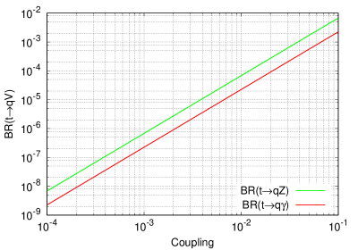
Figure 1: Branching ratios for decay channels $t\to q\gamma$ and $t\to qZ$ depending on the FCNC coupling.

The dominant SM decay mode of top quark is $t\to W^{+}b$, the decay width for this mode is given as

$$\Gamma(t\to W^{+}b)=\frac{\alpha|V_{tb}|^{2}}{16s_{W}^{2}}\frac{m_{t}^{3}}{m_{W}^{2}}(1-3m_{W}^{4}/m_{t}^{4}+2m_{W}^{6}/m_{t}^{6})$$ (3)

at the leading order (LO), and it is improved to the next to leading order (NLO) expression as given in Ref. Li91 . The ratios of the SM decay widths are calculated as $\Gamma(t\to W^{+}s)/\Gamma(t\to W^{+}b)\simeq|V_{ts}|^{2}/|V_{tb}|^{2}\simeq 1.495\times 10^{-3}$ and $\Gamma(t\to W^{+}d)/\Gamma(t\to W^{+}b)\simeq|V_{td}|^{2}/|V_{tb}|^{2}\simeq 6.318\times 10^{-5}$ Tanabashi18 . The top quark FCNC partial decay widths are

$$\Gamma(t\to q\gamma)=\frac{\alpha}{4}(\lambda_{qL}^{2}+\lambda_{qR}^{2})m_{t}$$ (4)

for the $t\to q\gamma$ channel, while the other partial decay widths are

$$\Gamma(t\to qZ)=\frac{\alpha}{32s_{W}^{2}c_{W}^{2}m_{Z}^{2}}(\kappa_{qL}^{2}+\kappa_{qR}^{2})m_{t}^{3}(1-m_{Z}^{2}/m_{t}^{2})(2-m_{Z}^{2}/m_{t}^{2}-m_{Z}^{4}/m_{t}^{4})$$ (5)

for the $t\to qZ$ channel, where $q=u,c$. The branching ratios for $t\to q\gamma$ and $t\to qZ$ decay channels depending on the FCNC $tq\gamma$ and $tqZ$ couplings are shown in Fig. 1.

III Sensitivities at Future ep Colliders

The production subprocess ($e^{-}q\to e^{-}W^{+}b$, where $q=u$,$c$) including signal diagrams with $tq\gamma$ and $tqZ$ interaction vertices is presented in Fig. 2. The similar diagrams for the subprocess ($e^{-}\bar{q}\to e^{-}W^{-}\bar{b}$) have also been included in the calculation. The cross sections for the process $e^{-}p\to e^{-}W^{\pm}q+X$ at different values of couplings $\kappa_{q}$ and $\lambda_{q}$ in the range of $(0.00-0.05)$ at LHeC and FCC-he are given in Table 1. The cross section increases when the coupling parameters $\kappa_{q}$ and $\lambda_{q}$ grow in the interested range. We plot the contours using Table 1 to estimate the sensitivity to FCNC coupling parameters. The contour lines correspond to different values of the signal cross sections (where $\Delta\sigma$ denotes the signal cross section (in pb) when the interfering background cross section is subtracted from the total cross section) as shown in Fig. 3 for LHeC and FCC-he. For a cross section value of the signal the sensitivity to coupling parameter $\lambda_{q}$ is higher than the coupling parameter $\kappa_{q}$.

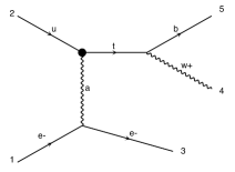
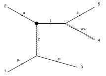
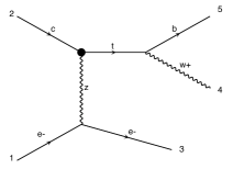
Figure 2: Diagrams including top quark FCNC $tq\gamma$ and $tqZ$ interaction vertices.

Table 1: The cross section values (in pb) for process $e^{-}p\rightarrow e^{-}W^{\pm}q+X$ at LHeC depending on different values of the couplings. The numbers in parenthesis denote the cross sections (in pb) at FCC-he.

Couplings		$\lambda_{q}$ = 0.00		$\lambda_{q}$ = 0.01		$\lambda_{q}$ = 0.02		$\lambda_{q}$ = 0.03		$\lambda_{q}$ = 0.05
$\kappa_{q}$ = 0.00		2.3000 (8.6100)		2.3094 (8.6421)		2.3365 (8.7275)		2.3805 (8.8737)		2.5213 (9.3411)
$\kappa_{q}$ = 0.01		2.3043 (8.6251)		2.3136 (8.6574)		2.3236 (8.7445)		2.3852 (8.8914)		2.5268 (9.3636)
$\kappa_{q}$ = 0.02		2.3135 (8.6646)		2.3406 (8.6956)		2.3505 (8.7899)		2.3957 (8.9344)		2.5387 (9.4088)
$\kappa_{q}$ = 0.03		2.3286 (8.7324)		2.3390(8.7659)		2.3666 (8.8518)		2.4123 (9.0031)		2.5559 (9.4776)
$\kappa_{q}$ = 0.05		2.3782 (8.9341)		2.3885 (8.9725)		2.4173 (9.0690)		2.4639 (9.2270)		2.6082 (9.7070)

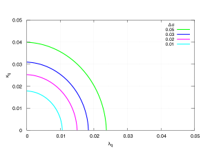
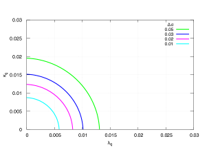
Figure 3: Contour plot for the top quark FCNC couplings $\kappa_{q}$ and $\lambda_{q}$ depending on the values (in pb) of signal cross sections at LHeC (left) and FCC-he (right).

The process $e^{-}p\to e^{-}W^{\pm}q+X$ includes both the signal and the background interfering with the signal. We calculate the cross sections for this process to normalize the distributions from the signal and background events. We take into account the main background (B1: $e^{-}W^{\pm}q$) and include other background (B2: $e^{-}Zq$) which contain at least three jets and one electron in the final state. Here, QCD multijet backgrounds are not included in the analysis of top quark FCNC $tq\gamma$ and $tqZ$ interactions.

In our calculations, we produce signal and background events by using MadGraph 5_aMC@NLO (MadGrapH2, ), with an effective Lagrangian implementation through FeynRules (FeynRules3, ) for the signal. Afterwards the parton showering and detector fast simulations are carried out with Pythia 6 (Pythia4, ) and Delphes 3.4 (Delphes5, ), respectively.

The kinematical distributions for signal and interfering background are given in Fig. 4 for LHeC and FCC-he. The transverse momentum ($p_{T}$) (on the left) and rapidty ($\eta$) (on the right) distributions of the leading jet, second leading jet and third leading jet are presented in these figures. These distributions are obtained after preselection of the events. For the analysis of signal and background events, we also apply analysis cuts after the generator level pre-selection. In order to select signal events we require having one electron and three jets ordered according to the highest transverse momentum $p_{T}$. Since there is an energy asymmetry in the electron-proton collisions, the jets from the process mainly peaks in the backward region, hence the pseudo-rapidy range for jets is taken as $-4<\eta<0$ in the analysis. The transverse momentum $p_{T}$ and pseudo-rapidty $\eta$ distributions of signal and main background have quite similar behaviour since we deal with small couplings for the signal and we take into account the interference of signal and background as well. In Fig. 5, the kinematical distributions ($p_{T}$ and $\eta$) of electron in the events are depicted. One of the specific aspects of the signal is the occurrence of the high $p_{T}$ electron in the central $\eta$ region.

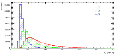
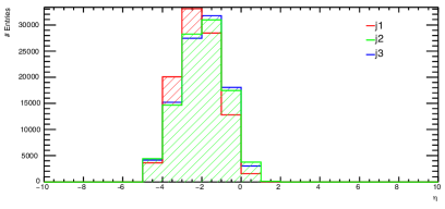
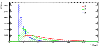
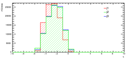
Figure 4: Transverse momentum ($p_{T}$) and pseudo-rapidity ($\eta$) distributions of three jets from the process $e^{-}p\rightarrow e^{-}W^{\pm}q+X$ which includes both the interfering background and signal for $\kappa_{q}$ = $\lambda_{q}$ = 0.05 at LHeC (first row) and FCC-he (second row).

In the analysis, we require at least three jets and one electron in the events, one of the jets should be $b$-tagged with leading jet $p_{T}(j)>40$ GeV and other jets having $p_{T}(j)>30$ GeV and $\mid\eta(j)\mid<2.5$, the electron with $p_{T}(e)>20$ GeV and $\mid\eta(e)\mid<2.5$ as the cut flow given in Table 2. Further steps in the cut flow table include invariant mass intervals for selecting events for the analysis.

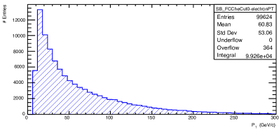
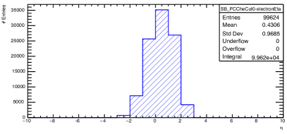
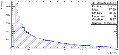
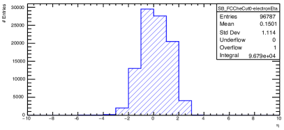
Figure 5: Transverse momentum and pseudo-rapidity distributions of electron from the process $e^{-}p\rightarrow e^{-}W^{\pm}q+X$ which includes both the interfering background and signal for $\kappa_{q}$ = $\lambda_{q}$ = 0.05 at LHeC (first row) and FCC-he (second row).

Table 2: Preselection and a set of cuts for the analysis of signal and background events.

Cuts				Definition
Cut-0				Preselection: $N_{jets}>=$ 3 and $N_{e}>=$ 1
Cut-1				$b-$tag: one $b-$tagged jet ($j_{b}$)
Cut-2				Transverse momentum: $p_{T}(j_{2},j_{3})>$ 30 GeV and $p_{T}(j_{b})>$ 40 GeV and $p_{T}(e)>$ 20 GeV
Cut-3				Pseudo-rapidity: -4 $<\eta(j_{b},j_{2},j_{3})<0$ and $|\eta(e)|<$ 2.5
Cut-4				$W$ boson mass: 50 $<M_{inv}^{rec}(j_{2},j_{3})<$ 100 GeV
Cut-5				Top quark mass: 130 $<M_{inv}^{rec}(j_{b},j_{2},j_{3})<$ 200 GeV

The cut efficiencies have been calculated after pre-selection for signal and background as shown in Fig. 6 for LHeC and FCC-he. We have larger cut efficiencies for higher values of the FCNC couplings. Fig. 6 shows that the cut efficiency for the background changes from $6\%$ to $1\%$ for Cut-1 to Cut-5, whereas the cut efficiencies for the signal decrease from $11\%$ to $3.2\%$ for couplings $\kappa_{q}=\lambda_{q}=0.05$.

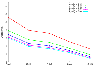
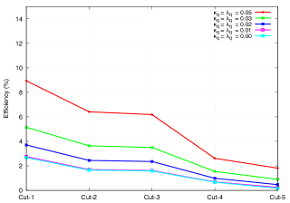
Figure 6: Efficiency plot for the cuts applied at each step for the analysis of signal and background at LHeC (left) and FCC-he (right).

After Cut-5, the number of events for background and signal (different values of couplings $\kappa_{q}$ and $\lambda_{q}$) are given in Table 3 for LHeC and for FCC-he with an integrated luminosity of $100$ fb^-1. For the coupling parameters $\kappa_{q}=\lambda_{q}=0.05$ we obtain the number of events 2153 (2844), while the background events are 508 (231) at LHeC (FCC-he). Thus, the signal gives an enhancement factor of 3.24 over the background for $\kappa_{q}=\lambda_{q}=0.05$, whereas this factor is 0.17 for $\kappa_{q}=\lambda_{q}=0.01$. For each cut step the number of events can be obtained from Table 3 with the relative cut efficiency factors from Fig. 6.

Table 3: The number of events for main background (where $\kappa_{q}=0$ and $\lambda_{q}=0$ ) and signal (where $\kappa_{q}\neq 0$ and $\lambda_{q}\neq 0$) with different FCNC couplings $\kappa_{q}$ and $\lambda_{q}$ at LHeC and FCC-he with L${}_{int}=$ 100 fb^-1. The numbers in parenthesis denote the number of events at FCC-he.

Couplings		$\lambda_{q}$ = 0.00		$\lambda_{q}$ = 0.01		$\lambda_{q}$ = 0.02		$\lambda_{q}$ = 0.03		$\lambda_{q}$ = 0.05
$\kappa_{q}$ = 0.00		508 (231)		558 (269)		670 (462)		894 (809)		1469 (1765)
$\kappa_{q}$ = 0.01		549 (259)		595 (334)		741 (491)		901 (834)		1624 (1818)
$\kappa_{q}$ = 0.02		622 (421)		646 (466)		779 (647)		971 (998)		1633 (1932)
$\kappa_{q}$ = 0.03		721 (576)		765 (703)		834 (915)		1113 (1286)		1841 (2227)
$\kappa_{q}$ = 0.05		1037 (1292)		1120 (1407)		1256 (1652)		1514 (1921)		2153 (2844)

We plot the invariant mass distribution of top quark reconstructed from three jets (one of them is $b-$tagged) for different coupling scenarios (at first row) $\lambda_{q}=0.0,\kappa_{q}=0.05$, (second row) $\lambda_{q}=0.05,\kappa_{q}=0.0$ and (third row) $\lambda_{q}=0.05,\kappa_{q}=0.05$ as shown in Fig. 7 for LHeC and FCC-he. The ratio of the $S+B$ and $B$ is more enhanced at top mass for equal coupling scenario (c) when it is compared with the other scenarios (a) and (b) as seen from Fig. 7.

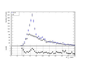
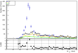
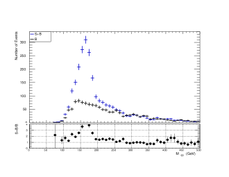
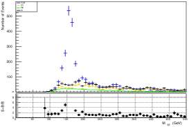
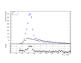
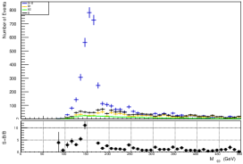
Figure 7: Invariant mass distributions of three jets (one of the jets is required as b-jet) for the signal + background (S+B) where B is the main background at LHeC (first column) and FCC-he (second column). First plot is for $\lambda_{q}=0,\>\kappa_{q}=0.05$ , second plot is for $\lambda_{q}=0.05,\>\kappa_{q}=0$ and third plot is for $\lambda_{q}=\kappa_{q}=0.05$.

In order to quantify statistical significance ($SS$), we calculate signal ($S$) and background ($B$) events after final cut. Here the $SS$ is defined by

$$SS=\sqrt{2[(S+B)\ln(1+\frac{S}{B})-S]}$$ (6)

The $SS$ values depending on the integrated luminosity ranging from 1 fb^-1 to 1 ab^-1 at the LHeC and FCC-he are presented in Fig. 8 for the coupling scenarios (at first row) $\lambda_{q}=0.0,\,\kappa_{q}=0.05$, (second row) $\lambda_{q}=0.05,\kappa_{q}=0.0$ and (third row) $\lambda_{q}=0.05,\kappa_{q}=0.05$. The significance corresponding to $2\sigma$, $3\sigma$ and $5\sigma$ lines (dotted) are also shown in these figures. In Fig. 8, the $SS$ values depending on the integrated luminosity ranging from $1$ fb^-1 to $1$ ab^-1 at the FCC-he are presented for these coupling scenarios with the $2\sigma$, $3\sigma$ and $5\sigma$ significances.

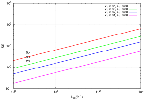
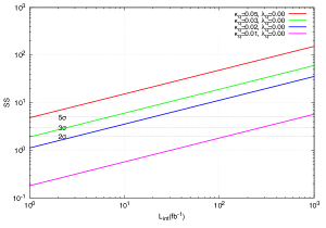
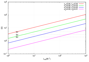
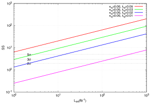
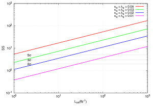
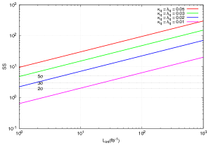
Figure 8: The statistical significance (SS) for the integrated luminosity ranging from 100 fb^-1 to 1 ab^-1 at the LHeC (first column) and FCC-he (second column). It includes the contribution from the main backgrounds on the predicted results. First row shows SS plot for $\lambda_{q}=0$ while $\kappa_{q}$ changes, second row is for $\kappa_{q}=0$ while $\lambda_{q}$ changes, and third row shows equal coupling scenario $\kappa_{q}=\lambda_{q}$.

Using the corresponding statistical significances, we fit the significance as a function of two parameters $\kappa_{q}$ and $\lambda_{q}$ at the integrated luminosity of $100$ fb^-1 and $1$ ab^-1. We obtain contour lines from the fit procedure. In Fig. 9, we estimate the reach for couplings $\kappa_{q}$ and $\lambda_{q}$ corresponding to $2\sigma$, $3\sigma$ and $5\sigma$ significance for integrated luminosity at the LHeC and FCC-he, respectively. We obtain the $2\sigma$ significance for the couplings $\kappa_{q}=0.014$, $\lambda_{q}=0.012$ and $\kappa_{q}=0.008$, $\lambda_{q}=0.007$ at LHeC with the integrated luminosities $100$ fb^-1 and $1$ ab^-1, respectively. The sensitivities to the couplings are enhanced at FCC-he as the obtained values $\kappa_{q}=0.008$, $\lambda_{q}=0.006$ and $\kappa_{q}=0.0037$, $\lambda_{q}=0.0025$ for $L_{int}=100$ fb^-1 and $1$ ab^-1, respectively.

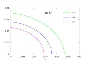
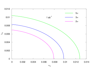
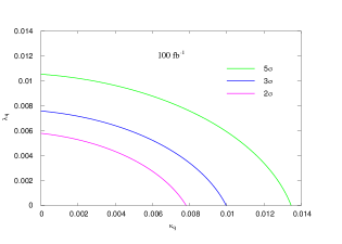
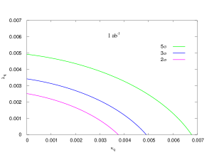
Figure 9: The reach of proposed couplings at different significance level at LHeC (first row) and FCC-he (second row) with luminosity projections 100 fb^-1 and 1 ab^-1.

The limits on couplings can be translated into the branching ratio via Fig. 1. We find the upper limits on branching ratio BR($t\to qZ$)$\leq 4.0\times 10^{-5}$ and BR($t\to qZ$)$\leq 1.0\times 10^{-5}$ at $2\sigma$ significance level for $L_{int}=1$ ab^-1 at LHeC and FCC-he, respectively. The HL-LHC will produce a large number of top quarks, which also provide opportunity to search for FCNC processes to improve existing constraints on the branching ratios BR($t\to qZ$)$<10^{-5}$ with the upgraded LHC experiments. We find better limits when compared to the current experimental limits and estimations for HL-LHC. In our previous studies given in Refs. ICakir2017 and Denizli17 , we have obtained the limits on the top quark FCNC $tq\gamma$ couplings depending on the integrated luminosity of future ep colliders. As a complementary to these studies, here we have analyzed both $tq\gamma$ and $tqZ$ couplings in three different scenarios and obtained sensitivities to the couplings $\kappa_{q}$ and $\lambda_{q}$.

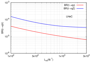
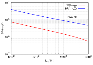
Figure 10: Expected sensitivities on BR($t\to q\gamma$) and BR($t\to qZ$) as a function of the integrated luminosity at LHeC (left) and FCC-he (right).

Finally, extending the analysis for higher luminosities, we present the expected sensitivities on BR($t\to q\gamma$) and BR($t\to qZ$) as a function of the integrated luminosity (in the range between 100 fb^-1 and 3000 fb^-1) at the LHeC and FCC-he in Fig. 10. For the integrated luminosities of 1 ab^-1, 2 ab^-1 and 3 ab^-1, the sensitivities on BR$(t\to q\gamma)$ and BR$(t\to qZ)$ are given in Table 4 at the LHeC and FCC-he.

Table 4: The sensitivities to the branching ratios BR($t\to q\gamma$) and BR($t\to qZ$) for three different luminosity projections at LHeC and FCC-he.

Collider		LHeC
Luminosity		1 ab-1		2 ab-1		3 ab-1
BR($t\to q\gamma$)		$1.0\times 10^{-5}$		$7.5\times 10^{-6}$		$6.2\times 10^{-6}$
BR($t\to qZ$)		$4.0\times 10^{-5}$		$3.5\times 10^{-5}$		$3.3\times 10^{-5}$

		FCC-he
		1 ab-1		2 ab-1		3 ab-1
		$1.5\times 10^{-6}$		$8.5\times 10^{-7}$		$5.5\times 10^{-7}$
		$9.5\times 10^{-6}$		$6.0\times 10^{-6}$		$4.5\times 10^{-6}$

IV Conclusion

The top quark FCNC interactions are important probes for new physics beyond the SM. It is also worth to mention that the analysis include the signal and background interference effects. The physics potential of future $ep$ colliders LHeC and FCC-he for probing new physics through top FCNC is promoted with their expected complementarity to the future lepton and hadron colliders. Sensitivities have been achieved for the $tq\gamma$ and $tqZ$ FCNC couplings at the LHeC with the center of mass energy of $1.3$ TeV and integrated luminosities of $L_{int}=1$ ab^-1, 2 ab^-1 and 3 ab^-1. The FCC-he with higher center of mass energy of $3.5$ TeV will allow us to significantly improve the sensitivity to the top quark FCNC.

V Acknowledgement

This work was partially supported by Bolu Abant Izzet Baysal University Scientific Research Projects under the project no: 2018.03.02.1286. Authors’ work was partially supported by Turkish Atomic Energy Authority (TAEK) under the project grant no. 2018TAEK(CERN)A5.H6.F2-20.

References

- (1) N. Cabibbo, Phys. Rev. Lett. 10, 531 (1963).
- (2) M. Kobayashi and T. Maskawa, Prog. Theor. Phys. 49, 652 (1973).
- (3) S. L. Glashow, J. Iliopoulos and L. Maiani, Phys. Rev. D 2, 1285 (1970).
- (4) ATLAS Collaboration, Eur. Phys. J. C 76, 55 (2016).
- (5) CMS Collaboration, Journal of High Energy Physics 04, 035 (2016).
- (6) M. Aaboud et al., ATLAS Collaboration, Journal High Energy Phys. 1710, 120 (2017).
- (7) A.M. Sirunyan et al., CMS Collaboration, JHEP 1707, 003 (2017).
- (8) ATLAS Collaboration, ATLAS Note ATL-PHYS-PUB-2013-007 (2013).
- (9) ATLAS Collaboration, ATLAS Note ATL-PHYS-PUB-2016-019 (2016).
- (10) J.A. Aguilar-Saavedra, Eur. Phys. J. C 77, 769 (2017).
- (11) J.L. Abelleria Fernandez et al., LHeC Study Group, Journal of Physics G: Nuclear and Particle Physics, vol. 39, Article ID 075001 (2012).
- (12) More information is available on the FCC web site: https://fcc.web.cern.ch.
- (13) I. Turk Cakir, A. Yilmaz, H. Denizli, A. Senol, H. Karadeniz and O. Cakir, Advances in High Eenergy Physics, vol. 2017, 1572053, 1-8 (2017).
- (14) H. Denizli, A. Senol, A. Yilmaz, I. Turk Cakir, H. Karadeniz, O. Cakir, Phys. Rev. D 96, 015024 (2017).
- (15) M. Kumar et al., Phys. Lett. B 764, 247 (2017).
- (16) C.S. Li, R.J. Oakes, and T.C. Yuan, Phys. Rev. D 43, 3759 (1991).
- (17) M. Tanabashi et al. (Particle Data Group), Phys. Rev. D 98, 030001 (2018).
- (18) J. Alwall et al., Journal of High Energy Physics 07, 079 (2014).
- (19) A. Alloul, N. D. Christensen, C. Degrande, C. Duhr, and B. Fuks, Computer Physics Communications, vol. 185, no. 8, pp. 2250–2300 (2014).
- (20) T. Sjostrand, S. Mrenna, and P. Skands, “PYTHIA 6.4 physics and manual,” Journal of High Energy Physics, vol. 5, article 026, (2006).
- (21) J. de Favereau et al., Journal of High Energy Physics, vol. 2014, article 57 (2014).