Minimal Re-computation for Exploratory Data Analysis in Astronomy

Abstract

We present a technique to automatically minimise the re-computation when a data analysis program is iteratively changed, or added to, as is often the case in exploratory data analysis in astronomy. A typical example is flagging and calibration of demanding or unusual observations where visual inspection suggests improvement to the processing strategy. The technique is based on memoization and referentially transparent tasks. We describe the implementation of this technique for the CASA radio astronomy data reduction package. We also propose a technique for optimising efficiency of storage of memoized intermediate data products using copy-on-write and block level de-duplication and measure their practical efficiency. We find the minimal recomputation technique improves the efficiency of data analysis while reducing the possibility for user error and improving the reproducibility of the final result. It also aids exploratory data analysis on batch-schedule cluster computer systems.

1 Introduction

Notwithstanding the notable successes in automating the reduction and analysis of data from radio telescopes, the traditional astronomer-driven data reduction is still common. This typically takes the form of exploratory, iterative, data reduction where visual inspection of intermediate or final data products is used to adjust, or add to, the data processing program. Each adjustment is typically small and impacts only a subset of the processing as a whole; however in current systems there is no way automatically re-run only this subset. Instead the user has the choice to either re-run the whole program, which can take minutes, hours or even days; or to manually do the sub-selection of the part of the program which needs to be re-run and risk introducing errors.

The situation can be easily be improved as we show below, by thin wrappers around existing data reduction software systems and applying techniques used in other parts of software engineering. We expect the benefits will be the greatest during telescope commissioning, during which the automated pipelines are being developed, and to particularly demanding observations where careful inspection of flagging, calibration, CLEANing and uv-weighting may be needed.

Similar workflows are encountered in optical observational astronomy as well as in general in data analysis. The reason for focusing on radio-astronomy are very large data-volumes (e.g., a number of radio telescopes record at a rate of excess of 1 TeraByte/hour) combined with complex data analysis which is made up out of a number of simpler tasks. The complexity of analysis in radio astronomy stems from:

1. Use of self-calibration [Pearson and Readhead, 1984]: iteratively solving for calibration solutions while simultaneously improving the estimated image of the sky

2. Iterative flagging of bad data

3. Use of user-supplied explicit constraints during deconvolution (‘CLEAN boxes’).

Self-calibration is illustrated in the sample program shown in 1.

2 Objective

The use case we consider is an astronomer who is repeatedly running a data reduction processing job with some change to the processing logic between each run. The primary objective is that, without any intervention from the astronomer, only the processing steps whose results could have changed (because either their parameters or their input data changed) are re-executed between the runs. We assume the processing logic is captured in a ‘script’ and the above implies astronomer does not need to edit the script in any way to select steps which are to be executed – instead the script as a whole is submitted for every execution.

The rationale for this objective is to, at the same time, improve the efficiency of data analysis (both in term of the computing time and the time of the astronomers doing the analysis) while reducing the possibility of errors resulting from astronomers manually sub-selecting parts of the script to be run. By only having a single script whose logic is incrementally improved we expect reproducibility and understandability will be improved.

The second objective is that the syntax and semantics of the scripts are as similar as possible to what astronomers are familiar with. In the field of radio astronomy at least this means Python, or Python-like syntax and semantics. The rationale for this is to maximise of the uptake of this software – very few would be willing to learn a new paradigm of computing.

The third objective is to enable modularity of the scripts. The rationale is that as exploitative analysis becomes more driven by complete scripts those scripts will become increasingly complex and it will be desirable to have modularity to make them easier to construct and to read.

3 Approach

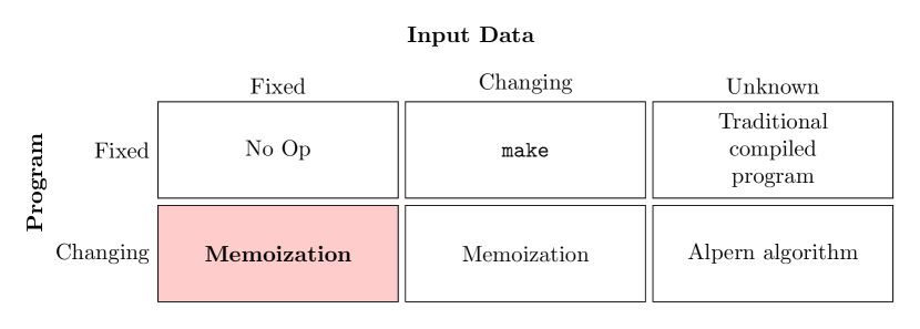
Figure 1: Classification of techniques for minimising computation for all combinations of changing program and data scenarios. The primary scenario we consider here the box shaded red – input data are fixed and the program is changing.

Minimal re-computation can be classified based on whether re-computation happens after a change in the data input or a change in the program itself. Specifically, the program can be considered either to be ‘fixed’ or to be ‘changing’ and the data can be considered to be either ’fixed’, ’changing’ or ‘unknown’. The ‘unknown’ category for data is useful because some program changes can be proven not to affect the output regardless of what data are input. This classification is illustrated graphically in Fig 1.

In the scenario we consider here the input data are known and fixed – they are the raw data recorded by the telescope – while the data processing program is evolving between processing runs. This scenario can be contrasted with one where the program does not change but some of the input data changes between runs: the classic example of this is the make program which minimises the re-compilation/re-linking when a subset of source code files changes. Another scenario considered in previous work [Small et al., 2015] is where the input data are unknown, i.e., the minimal set of re-computation needs to be determined without reference to a particular input data.

The approach we adopt is to have referentially transparent tasks at the user level and use memoization. A referentially transparent task is a task whose call can always be replaced by its return values. The important implications for astronomy are that tasks cannot have observable side effects other then their return values and that tasks can not modify in-place any of their input variables. So for example, a task to calibrate a dataset must return a new calibrated dataset rather than modifying the dataset it has been passed. The downside of such tasks is that a processing job will require more disk storage space; we describe below how we ameliorate this.

Memoization [Michie, 1968, Abelson et al., 1996] is the technique of tabling the results of task invocations against their inputs. In astronomy this means tabling the results against both the input astronomical data and any adjustable processing parameters. The technique is commonly used in functional programming languages or when a functional sub-set of a language is used. A well known example is Packrat parsing [Ford, 2002]. The downside of memoization is the storage space required for keeping the results, which we limit with an eviction strategy described below. Another downside in the general case is the high cost of lookup for extremely fine grained tasks but this is unlikely to apply to typical astronomical processing scripts and their tasks. The approach we adopt parallels that put forward in some other fields in software engineering: we list these related works in Section 7. As far as we are aware this is the first time a technique of this type has been applied to scientific data analysis.

4 Design & Implementation

The software system we implemented is named Recipe and in this work we concentrate on using it in cojuction with CASA [McMullin et al., 2007], probably the widest-used software package in radio astronomy. A similar approach can easily be applied to ParselTongue [Kettenis et al., 2006] as we showed earlier [Small et al., 2015]. The strategy we adopt is to wrap the existing CASA interface to make it referentially transparent and to replace the use of user-defined filenames with automatically generated unique strings (which the user handles via Python variables rather than explicitly). We then apply memoization to this new interface, storing the tabling key as the filename of the value. Values are evicted according the Least-Recently-Used (LRU) strategy. An outline of the algorithm is shown in Figure 2.

Figure 2: Flow diagram illustrating the algorithm used for minimal re-computation applied to CASA workflows as implemented by the recipe system.

Users interact with CASA predominately via “tasks”, a Python-based interface where input and output data are always files on disk. This interface is functional in the sense no state is retained in memory between task invocations. CASA tasks however often create their outputs by modifying their input datasets, thus invalidating the input dataset for use in substituting out some previous computation. We make such tasks suitable for minimal re-computation by copying the input dataset before the task is invoked and using this copy as the output value of the task.

Since some tasks only modify a small part of the input dataset, this copy approach can be inefficient on traditional filesystems. For this reason we use OpenZFS (on Linux) which supports block-level de-duplication or BTRFS which supports file-level Copy-On-Write (COW). With both of those approaches, a copy of a file (i.e., not just a link to) will not cause any copying of the on-disk blocks until those specific blocks have been changed for the first time. In the present case this means that when a task modifies its input dataset, only the blocks it modifies will actually use disk space. The savings in disk space due to the use of copy-on-write or de-duplication are measured in Section 5.

In normal usage, CASA users specify the files which contain inputs and outputs of tasks directly by their concrete filenames. Multiple approaches can be used to apply memoization in this situation. One approach is to hash the input datafiles and use hashes for tabling; another is to infer the dataflow [see Small et al., 2015, for a description]. The approach we adopt is to encourage the analyst to use variables instead of direct filenames, and to ensure the actual filenames are the string representations of the hash of the task call that was used to generate their contents. This approach has two advantages: no hashing of file contents is needed (a potentially expensive operation) as long as raw input data have stable filenames and are never modified in-place (the normal situation in radio-astronomy); and, the resulting code structure is much easier to modularise since the file variables are lexically scoped in the same way as the other variables. By contrast, direct use of filenames is equivalent to a single global namespace for file variables.

Memoized values are checked for eviction before every call into a task. The trigger is the free disk space on the filesystem used to store the values, i.e., values will be evicted if the free space is less than a certain critical value. The criterion used is the last-access time stamp of the files. This implements the least-recently-used cache eviction scheme. When a task checks for the existence of a memoized value, it updates the last-access time even if the value is not read (i.e., the descendant task has also been memoized) – this is done in order to reduce the chance of early eviction of roots of long, deep dataflows.

Complete information, source code and links to the Git revision control repository for the full implementation is available at http://www.mrao.cam.ac.uk/~bn204/sw/recipe. Introspection facilities of Python and regularity of the CASA task interface means that only around 150 lines of Python are required for the implementation.

A reduced example script using this implementation is shown in Listing1. This script implements iterative self-calibration on the Galactic Centre for HERA as described by Nikolic and Carilli [2017]. The only differences to typical CASA/Python scripts are:

1. Filenames are never specified explicitly by the analyst except for the input data (which are assumed not to change)

2. Every wrapped CASA task returns a single value which is the filesystem path containing the output of the task

We have found analysts familiar with CASA are able to use the minimal re-computation framework with little training.

In Table 1 we present a comparison the run time performance of our minimal re-computation software versus plain CASA. The workload used is a typical self-calibration workload, consisting of a slightly extended version of the script in Listing1. It can be noted that:

1. On the initial run, performance of Recipe/CASA is close to, but slightly better than plain CASA. This is because the automatic re-use of some intermediate data product in the self-calibration loop outweighs the time for some additional copying of data that minimal recomputation requires.

2. On subsequent runs of the same script the performance of Recipe/CASA is extremely high as only cache queries corresponding to checking of existence of a file need to be made. As there is no need to list the whole cache directory, the performance is not expected to degrade appreciably with increasing cache size.

5 Practical de-duplication and copy-on-write efficiency

We have measured the efficiency (with respect to the volume of storage required) of both the de-duplication and copy-on-write approaches. The measurement was made with a slightly expanded version of program in Listing 1 with input data consisting of a single HERA observation with 40 antennas. The size of the input dataset is 1.8 GB and size of the complete repository for intermediate data products is 41 GB. All tests were done with CASA version 5.1 using standard Measurement Set V2 files on GNU/Linux Ubuntu 17.04 Kernel 4.10 with both ZFS (for de-duplication) and BTRFS (for copy-on-write).

When using ZFS block-level de-duplication the allocated space on disk is 6.5 GB and the de-duplication factor $6.2\times$ (both as reported by the zpool list command). Some copying of data is unavoidable in normal manual CASA processing, this shows that with de-duplication is highly efficient for this problem, and that the repository is only perhaps two times larger than would be necessary at the minimum. ZFS de-duplication however requires a significant reserve of RAM to function efficiently as it needs to maintain a table with the check-sums of all of the blocks.

In the same test environment we measured the efficiency of the copy-on-write mechanism provided by BTRFS. For this purposes all copies were done with cp --reflink=auto flag. We find disk usage is 8.4 GB, a saving of $4.9\times$ compared to no copy-on-write. Therefore, the copy-on-write mechanism is less efficient than de-duplication, but still very good. The advantage of copy-on-write compared to de-duplication is that it does not impose additional RAM memory requirements. In most general purpose scenarios we expect the copy-on-write approach would give sufficient storage efficiency without additional hardware requirements.

6 Minimal re-computation in a batch-scheduled cluster environment

Analysis of data from large radio telescopes (e.g., ALMA, JVLA, LOFAR) is often done on shared-filesystem computer clusters. Such clusters are often batch-scheduled to facilitate efficiency, making interactive use impossible. Exploratory data analysis must then be done by submitting multiple data analysis scripts for processing which creates issues of many unnecessary re-computations and keeping track of the results of each script.

The proposed technique of minimal re-computation and the implementation we have created work on a multi-user shared-filesystems cluster without need for modification and with high efficiency. The key feature is the use of the filesystem as the only store of information, which being a shared resource on the cluster means that all computers see a synchronised version of the data. In particular, both multiple jobs and multiple users can re-use each other’s previously computed values regardless on which computer on the cluster they get scheduled on.

We find use of minimal recomputation significantly improves the work-flow of exploratory data analysis on a batch-scheduled cluster:

• It is efficient to submit initial parts of the script while later parts are being developed: the results of initial evaluation can then be available when the full script is submitted

• There is no need to constrain the scheduling of many similar scripts: they can be executed in any order and on any machine and will re-use each others intermediate values as available

• The enforced referential-transparency of tasks usefully aids modularisation which is more important when interactive use is not possible.

Configuration
Environment	Software	1st Execution	Repeated Execution
		Time	Time
Workstation	CASA	10m30s	10m29s
	Recipe/CASA	9m59s	0.1s
Cluster	CASA	16m37s	16m9s
	Recipe/CASA	19m37s	0.1s

Table 1: Results of measurement of execution time. The ‘Workstation’ environment is a Dell T7810 Single Node Dual Socket Xeon E5-2680 v3 with 64 GB ECC RAM with 4x Samsung SM961 512GB NVMe Storage organised as a striped ZFS filesystem. The ‘Cluster’ environment refers to University of Cambridge’s ‘CSD3’ cluster with Intel Skylake processors and a shared Lustre filesystem connected to OmniPath fabric. ‘Recipe/CASA’ refers to our minimal re-computation software driving CASA, as described in text. CASA version 5.3 for RHEL 7 was used. The script which was timed is a slightly extended version of 1 representing a realistic self-calibration processing in radio astronomy. All times are wall-clock times.

Measurement of run-time performance in the cluster environment is presented in Table 1 (together with single-node performance as described above). We note that overall execution time slower in the cluster. Experience suggests this primarily due to overheads of access to the data over the shared Lustre filesystem. We also note Recipe/CASA in the cluster environment is now slower than plain CASA: this is because the slower file-system access increases the overhead due to copying of data inherent in the minimal re-processing when some operations modify their input data. Nevertheless, the primary advantage of very fast repeated execution is clearly demonstrated in the cluster environment.

7 Related work

The most generally familiar related system is ccache. It minimises recompilation when both the source code and the instructions for compilation may be changing (e.g., due to edits to Makefiles or experimenting with different compilation switches). In this scenario the equivalent of our data analysis program are the Makefiles while the equivalent to our astronomical data is the program source code. Ccache is specialised for compilation only; also, in contrast to our system, it always reads the full input data (and also does pre-processing on them) before computing the hashes.

The most direct inspiration was the Ciel dataflow execution engine [Murray et al., 2011]. Another inspiration was the NiX [Dolstra, 2006] system, which like ccache works in the domain of software building, but applies the minimal re-computation methodology to building a whole Linux distribution rather than a single program. From NiX we take the idea of using the filesystem as a database keyed by the hash of the processing requested from each task.

A related system is Nectar described by Gunda et al. [2010]. It too uses the idea of a cache of intermediate results (or sub-expression values) to speed up program execution when the program is being developed, or shared by multiple users. It includes a sophisticated rewriting engine rather than simple memoization. Nectar is specialised on the LINQ data processing language working in the CLR environment, so would be difficult to integrate with software such as CASA. A similar related system is IncPy presented by Guo and Engler [2011], This system is also based on memoization, however it requires a modification to the Python interpreter in order to dynamically analyse dependencies of Python functions. It could not therefore be applied to CASA (which comes with own Python interpreter and accesses files from its C++ code). The system presented here additionally replaces all user-created files with unique values based on memoization hashes; this allows re-use of values across many previous generation of the analysis script.

8 Conclusions

We present an approach to minimal recomputation and a concrete implementation for the CASA radio astronomy data analysis system. The implementation can be adapted to other task-based astronomy data analysis applications which use the filesystem for storage of all input and output data. When used in combination with a copy-on-write filesystem, the technique has modest additional storage requirements while providing significant benefits in reproducability and efficiency of the data analysis. The benefits are amplified in batch-scheduled computer clusters where interactive use is difficult.

The approach presented here has implications on the design and implementation of data models used in science: models structured so that changes or additions to data change as few on-disk block as possible will provide highest efficiency in terms of storage requirements.

The technique here also significant bearing on ‘notebook-style’ interaction with programs, as first popularised by Wolfram Research’s Mathematica, and now often used in the field of scientific data analysis through the Jupyter system. In such systems, when an entry in a notebook is changed, the user usually has the options to either re-evaluate the whole notebook or try to singly evaluate all statements which my be affected by the first change. Minimal re-computation resolves this problem (subject to sufficient storage space) by allowing the user to always select re-evaluation the whole notebook while automatically only the statements which could have changed are actually re-evaluated.

References

Appendix A Example Recipe program

Listing 1: Self-calibration data reduction based on script for imaging data from the Hydrogen Epoch of Reionization Experiment (HERA). Multiple iterations of the self-call loop are made with different strategies (number of CLEAN iterations, gain versus bandpass calibration).

⬇

# Input, unchaging files

ingc="GCmodl.cl"

invis="exampleinputvis.ms"

# Insert model for first calibration

f1=ft(invis, complist=ingc, usescratch=True)

# Calculate delay calibration

K=gaincal(f1, gaintype=’K’)

# Calculate antenna based-gain errors

G=gaincal(f1, gaintable=[K], gaintype=’G’)

# Apply the initial solutions

f2=applycal(f1, gaintable=[K, G])

# Outputs can be assigned directly to other variables

f3=f2

# First clean, to setup a very simple model for the GC

ooorig=clean(vis=f3, niter=50)

# Example of a clean Module

def iterselfcal(visin, img, niter, dobandpass=False):

"""Make␣one␣iteration␣of␣the␣self␣cal␣loop

␣␣␣␣:param␣img:␣Image␣to␣use␣as␣the␣model

␣␣␣␣:param␣niter:␣Number␣of␣minor␣cycle␣iterations

␣␣␣␣:param␣dobandpass:␣Do␣a␣bandpass␣calibration␣?

␣␣␣␣"""

# Now back to the original vis for the calibration. NB. use the

# *model* output from previous here

f33=ft(visin,

model=os.path.join(img, "img.model"),

usescratch=True)

ctl=[]

K2=gaincal(f33, gaintype=’K’)

ctl.append(K2)

G2=gaincal(f33, gaintype=’G’, gaintable=[K2])

ctl.append(G2)

if dobandpass:

B2=bandpass(f33, bandtype="B", gaintable=ctl)

ctl.append(B2)

f33=applycal(f33, gaintable=ctl)

# Reclean

oo=clean(vis=f33, niter=niter)

return oo, ctl

# Incrementally CLEAN and re-solve for solutions, first with and then

# without bandpass

oo1 ,GG1=iterselfcal(f1, ooorig, 500)

oo11,GG2=iterselfcal(f1, oo1, 5000)

oo2 ,GG3=iterselfcal(f1, oo1, 500, dobandpass=True)

oo3 ,GG4=iterselfcal(f1, oo2, 5000, dobandpass=True)

References

- Abelson et al. [1996] Abelson, H., Sussman, G.J., Sussman, J., 1996. Structure and interpretation of computer programs. Justin Kelly.
- Dolstra [2006] Dolstra, E., 2006. The Purely Functional Software Deployment Model. Ph.D. thesis. IPA.
- Ford [2002] Ford, B., 2002. Packrat parsing: Simple, powerful, lazy, linear time. SIGPLAN Not. 37, 36–47. URL: http://doi.acm.org/10.1145/583852.581483, doi:10.1145/583852.581483.
- Gunda et al. [2010] Gunda, P.K., Ravindranath, L., Thekkath, C.A., Yu, Y., Zhuang, L., 2010. Nectar: Automatic management of data and computation in datacenters, in: OSDI: 9th USENIX Symposium on Operating Systems Design and Implementation.
- Guo and Engler [2011] Guo, P.J., Engler, D., 2011. Using automatic persistent memoization to facilitate data analysis scripting, in: Proceedings of ISSTA’11, ACM. ACM.
- Kettenis et al. [2006] Kettenis, M., van Langevelde, H.J., Reynolds, C., Cotton, B., 2006. ParselTongue: AIPS Talking Python, in: Gabriel, C., Arviset, C., Ponz, D., Enrique, S. (Eds.), Astronomical Data Analysis Software and Systems XV, p. 497.
- McMullin et al. [2007] McMullin, J.P., Waters, B., Schiebel, D., Young, W., Golap, K., 2007. CASA Architecture and Applications, in: Shaw, R.A., Hill, F., Bell, D.J. (Eds.), Astronomical Data Analysis Software and Systems XVI, p. 127.
- Michie [1968] Michie, D., 1968. Memo functions and machine learning. Nature 218, 19–22.
- Murray et al. [2011] Murray, D.G., Schwarzkopf, M., Smowton, C., Smith, S., Madhavapeddy, A., Hand, S., 2011. Ciel: A universal execution engine for distributed data-flow computing, in: Proceedings of the 8th USENIX Conference on Networked Systems Design and Implementation, USENIX Association, Berkeley, CA, USA. pp. 113–126. URL: http://dl.acm.org/citation.cfm?id=1972457.1972470.
- Nikolic and Carilli [2017] Nikolic, B., Carilli, C., 2017. Self-calibration of highly-redundant low-frequency arrays: Initial results with HERA, in: 2017 XXXIInd General Assembly and Scientific Symposium of the International Union of Radio Science (URSI GASS), pp. 1–4. doi:10.23919/URSIGASS.2017.8105387.
- Pearson and Readhead [1984] Pearson, T.J., Readhead, A.C.S., 1984. Image Formation by Self-Calibration in Radio Astronomy. ARA&A 22, 97–130. doi:10.1146/annurev.aa.22.090184.000525.
- Small et al. [2015] Small, D., Kettenis, M., Nikolic, B., 2015. Hilado Deliverable 10.13: A framework for minimal recomputation. Technical Report D10.13. EC RadioNet3 FP7 project. http://www.radionet-eu.org/radionet3wiki/lib/exe/fetch.php?media=jra:d10.13_rn3_deliverable_hilado_150602.pdf.