Time-optimality by distance-optimality for parabolic
control systems

Abstract.

The equivalence of time-optimal and distance-optimal control problems is shown for a class of parabolic control systems. Based on this equivalence, an approach for the efficient algorithmic solution of time-optimal control problems is investigated. Numerical examples are provided to illustrate that the approach works well is practice.

1. Introduction

This article is devoted to time optimal control problems for parabolic systems. Specifically, we propose a formulation which is equivalent to the original time optimal control formulation and amenable for numerical realization. We consider the problem

($$P \mbox{Minimize~{}}T\quad\text{subject to}\quad\left\{\begin{aligned} T&>0\mbox{,}\\ u&\in U_{ad}(0,T)\mbox{,}\\ \partial_{t}y+Ay&=Bu\mbox{,}&\mbox{in~{}}(0,T)\mbox{,}\\ y(0)&=y_{0}\mbox{,}\\ \lVert y(T)-y_{d}\lVert_{H}&\leq\delta_{0}\mbox{,}\\ \end{aligned}\right.$$)

where $y$ denotes the state, $u$ the control, and $T$ the terminal time. Here, the set of admissible controls is

$$U_{ad}(0,T)\coloneqq\left\{u\in L^{2}((0,T);L^{2}(\omega))\colon u_{a}\leq u(t)\leq u_{b}\mbox{~{}a.e.~{}}t\in(0,T)\right\}$$

for $u_{a},u_{b}\in L^{\infty}(\omega)$ the control constraints, where $\omega$ is a measurable set. Moreover, $A$ is an unbounded operator satisfying Gårding’s inequality and $B$ is the (bounded) control operator; see also Section 2 for the precise assumptions. The goal is to steer the system into a ball centered at $y_{d}$ with radius $\delta_{0}$ in the shortest time possible. Note that the state equation is posed on a variable time horizon which causes a nonlinear dependency of the state $y$ with respect to the terminal time $T$ and the control $u$. For this reason, ($P$) is a nonlinear and nonconvex optimization problem subject to control as well as state constraints. Additionally we emphasize that the objective functional does not contain control costs which complicates the algorithmic solution of ($P$) compared to the situation with an $L^{2}$ term in the objective; cf., e.g., [15, 18].

In this article, we propose an equivalent reformulation in terms of minimal distance problems that can be used algorithmically to solve the time-optimal control problem. For $\delta>0$ consider the perturbed time-optimal control problem defined as

($$P_{\delta} \inf_{\begin{subarray}{c}T>0\\ u\in U_{ad}(0,T)\end{subarray}}\;T\quad\text{subject to}\quad\lVert y[u](T)-y_{d}\lVert_{H}\leq\delta_{0}+\delta,$$)

where $y[u](T)$ denotes the state associated with the control $u$ evaluated at $T$. Moreover, we consider the minimum distance control problem

($$\delta_{T} \mbox{Minimize~{}}\lVert y[u](T)-y_{d}\lVert_{H}-\delta_{0}\quad\mbox{subject to}\quad u\in U_{ad}(0,T)\mbox{.}\\$$)

Under weak assumptions we show that the associated value functions defined by

$$T(\delta)=\inf\eqref{TOPT}\quad\text{and}\quad\delta(T)=\inf\eqref{DOPT}$$

are inverse to each other; see Proposition 3.4. Furthermore, we prove that ($P_{\delta}$) and ($\delta_{T}$) are equivalent. Precisely, if $\delta>0$ is given and $(T,\bar{u})$ is optimal for ($P_{\delta}$), then $\bar{u}$ is also distance-optimal for ($\delta_{T}$). Conversely, if $T>0$ is given and $\bar{u}$ is distance optimal, then $(T,\bar{u})$ is time-optimal with $\delta=\delta(T)$; see Theorem 3.1 for details. Hence, instead of solving the time-optimal control problem directly, we can search for a root of the $\delta(\cdot)$-value function. A similar equivalence first appeared in [35] (see also [34, Section 5.4]) for the situation where one aims at delaying the activation of the control as long as possible. However, to the best of our knowledge it has never been considered for an algorithmic approach. In this regard, we also mention a similar approach used in [11] for time-optimal control of a one-dimensional vibrating system with controls in a subspace of $L^{2}$ determined by certain moment equations.

We show that the $\delta(\cdot)$-value function is continuously differentiable for many important control scenarios; see Section 5. If in addition qualified optimality conditions hold for the original problem, then the derivative of $\delta(\cdot)$ is nonvanishing near the optimal solution; see Proposition 6.2. This justifies to use a Newton method for the calculation of a root of $\delta(\cdot)$. Moreover, under an additional assumption we show that the derivative of the value function is Lipschitz continuous which guarantees fast local convergence of the Newton method. In fact, in all our numerical examples, we observe quadratic order of convergence, even if the additional assumption does not hold. For the solution of the resulting minimal distance problem with simple control constraints, the literature offers a wide spectrum of algorithms.

Time optimal control problems are among the most studied problems of optimal control, and thus it comes at no surprise that diverse techniques have been proposed for their solution. In the following let us briefly describe some of them. An approach, which is conceptually close, rests on an equivalent reformulation utilizing minimum norm problems. In contrast, to the perturbations in the terminal constraint as in ($P_{\delta}$), perturbations in the control constraint are introduced. To explain the approach, we consider the time optimal control problem

($$P_{\rho} \inf_{\begin{subarray}{c}T>0\\ u\in L^{2}((0,T)\times\omega)\end{subarray}}\;T\quad\text{subject to}\quad\lVert y[u](T)-y_{d}\lVert_{H}\leq\delta_{0},\quad\lVert u\lVert_{L^{\infty}((0,T);L^{2}(\omega))}\leq\rho,$$)

which is related to the minimal norm problem defined as

($$N_{T} \inf_{u\in L^{2}((0,T)\times\omega)}\;\lVert u\lVert_{L^{\infty}((0,T);L^{2}(\omega))}\quad\text{subject to}\quad\lVert y[u](T)-y_{d}\lVert_{H}\leq\delta_{0}.$$)

To follow much of the literature, we adapted the control constraints to be chosen in $L^{\infty}((0,T);L^{2}(\omega))$ rather than $L^{\infty}((0,T)\times\omega)$. Under appropriate controllability assumptions these two problems have been shown to be equivalent; see [17, 8, 10, 36, 30] for parabolic equations, [38] for time-varying ordinary differential equations, [34, Chapter 5] for abstract evolution equations, and [39] for the Schrödinger equation. Note that typically these publications consider the case of exact controllability, i.e. $\delta_{0}=0$, or exact null controllability, i.e. $\delta_{0}=0$ and $y_{d}=0$. The solution to ($N_{T}$) can be determined by solving an unconstrained optimization problem given by

(1.1) $$\inf_{\varphi_{T}\in H}\frac{1}{2}\left(\int_{0}^{T}\lVert B^{*}\varphi(t)\lVert_{L^{2}(\omega)}\,\mathrm{d}t\right)^{2}+(\varphi(0),y_{0})+\delta_{0}\lVert\varphi_{T}\lVert_{H}-(y_{d},\varphi_{T}),$$

where $\varphi$ is the solution to the adjoint state equation

$$-\partial_{t}\varphi+A^{*}\varphi=0,\quad\varphi(T)=\varphi_{T};$$

see [30, Section 4], compare also [9, Section 1.7]. If $\bar{\varphi}_{T}$ is the minimizer of (1.1), then the minimum norm control is given by

$$\bar{u}(t)=\left(\int_{0}^{T}\lVert B^{*}\bar{\varphi}(t)\lVert_{L^{2}(\omega)}\,\mathrm{d}t\right)\frac{(B^{*}\bar{\varphi})(t)}{\lVert(B^{*}\bar{\varphi})(t)\lVert_{L^{2}(\omega)}},\quad\text{a.e.~{}}t\in(0,T),$$

where $\bar{\varphi}$ is the adjoint state with terminal value $\bar{\varphi}_{T}$. Turning to the numerical realization, as far as we know, the only algorithmic studies based on this equivalence are [21] for time-optimal control problems subject to ordinary differential equations and [24] for problems subject to partial differential equations employing an optimal design approach. A direct numerical realization of ($N_{T}$) is impeded by the difficulties related to the appearance of the state constraint and the fact that the minimization is carried out over a non-reflexive Banach space. In contrast (1.1) does not contain state constraints. Turning to the realization of ($N_{T}$) by means of (1.1), one has to cope with the non-smoothness of the $L^{1}$-norm, whereas ($\delta_{T}$) involves the minimization of a Hilbert space norm. In addition, (1.1) can be considered as an inverse source problem for the initial condition of the adjoint problem. Such problems are inherently ill-posed. For the specific context of (1.1) this was analyzed in [25].

An alternative approach to solve time-optimal control problems for finite or infinite dimensional systems is based on solving the optimality system for ($P$) after adding a regularization term of the form $\alpha\lVert u\lVert^{2}$ to the cost functional. In an additional outer loop the regularization parameter $\alpha$ can be driven to zero; see [15, 19, 18]. This is a flexible method, but one has to cope with the difficulties of the asymptotic behavior as the regularization parameters tends to zero. We compare our approach with the regularization approach in one numerical example and observe that even for a fixed regularization parameter our algorithm performs roughly five to ten times faster in terms of the required number of solves for the partial differential equation; see Table 3.

Yet another approach, which has mostly been investigated for time-optimal control problems subject to ordinary differential equations, rests on the reformulation of ($P$) as an optimization problem with respect to the switching points of the optimal controls; see, e.g., [16, 23]. This approach cannot be extended to the distributed control setting in a straightforward way.

This paper is organized as follows: In Section 2 we introduce the notation and main assumptions. The equivalence of time and distance optimal controls is proved in Section 3. Section 4 is devoted to general properties of the time-optimal control problem. Differentiability of the value function associated to the minimal distance problems is proved in Section 5. The algorithm is presented in Section 6. Various numerical examples in Section 7 show that our approach is efficient in practice. Last, in Section 8 we conclude with some open problems.

2. Notation and main assumptions

Let $V$ and $H$ be real Hilbert spaces forming a Gelfand triple, i.e. $V\hookrightarrow_{c}H\cong H^{*}\hookrightarrow V^{*}$, where $\hookrightarrow$ denotes the continuous embedding and $\hookrightarrow_{c}$ the continuous and compact embedding. We abbreviate the duality pairing between $V$ and $V^{*}$ as well as the inner product and norm in $H$ by

$$\langle\cdot,\cdot\rangle=\langle\cdot,\cdot\rangle_{V^{*},V},\quad(\cdot,\cdot)=(\cdot,\cdot)_{H},\quad\lVert\cdot\lVert=\lVert\cdot\lVert_{H}\mbox{.}$$

Assumption 2.1.

Let $a\colon V\times V\to\mathbb{R}$ be a continuous bilinear form, which satisfies the Gårding inequality (also referred to as weak coercivity): There are constants $\alpha_{0}>0$ and $\omega_{0}\geq 0$ such that

(2.1) $$a(v,v)+\omega_{0}\lVert v\lVert^{2}\geq\alpha_{0}\lVert v\lVert^{2}_{V}\quad\text{for all~{}}v\in V\mbox{.}$$

We denote by $A\colon V\subset V^{*}\to V^{*}$ the unique linear operator with

$$\langle Ay,v\rangle=a(y,v)\quad\text{for all~{}}v\in V.$$

The Gårding inequality implies that $-A$ generates an analytic semigroup on $V^{*}$ denoted $\mathrm{e}^{-\cdot A}$; see, e.g., [27, Section 1.4].

Assumption 2.2.

Let $(\omega,\varrho)$ be a measure space. We assume that the control operator $B\colon L^{2}(\omega,\varrho)\rightarrow V^{*}$ is linear and continuous. Moreover, $y_{d}\in H$ is the desired state and $\delta_{0}>0$.

The abstract measure space allows for one consistent notation for different control scenarios. For example, in case of a distributed control on a subset $\omega$ of the spatial domain $\Omega\subset\mathbb{R}^{d}$ we take $\omega$ equipped with the Lebesgue measure. If no ambiguity arises, we drop the measure $\varrho$ and simply write $\omega$ in the following. The space of admissible controls is defined as

$$U_{ad}\coloneqq\left\{u\in L^{2}(\omega)\colon u_{a}\leq u\leq u_{b}\;\mbox{~{}a.e.\ in~{}}\;\omega\right\}\subset L^{\infty}(\omega)$$

for $u_{a},u_{b}\in L^{\infty}(\omega)$ with $u_{a}<u_{b}$ almost everywhere. In addition, for $T>0$ we set $U(0,T)\coloneqq L^{2}((0,T)\times\omega)$ and

$$U_{ad}(0,T)\coloneqq\left\{u\in U(0,T)\colon u(t)\in U_{ad}\mbox{~{}a.e.~{}}t\in(0,T)\right\}\subset L^{\infty}((0,T)\times\omega),$$

where $(0,T)\times\omega$ is equipped with the completion of the product measure. For $T>0$ we use $W(0,T)$ to abbreviate $H^{1}((0,T);V^{*})\cap L^{2}((0,T);V)$, endowed with the canonical norm and inner product. The symbol $i_{T}\colon W(0,T)\rightarrow H$ denotes the trace mapping $i_{T}y=y(T)$. For any two Banach spaces $X$ and $Y$, let $\mathcal{L}(X,Y)$ denote the space of linear and bounded operators from $X$ to $Y$. The symbol $\mathcal{B}_{r}(x)$ stands for the ball centered at $x\in X$ with radius $r>0$ in $X$. Moreover, $\mathbb{R}_{+}$ abbreviates the open interval $(0,+\infty)$.

Last, to ensure the existence of optimal controls we require the following

Assumption 2.3.

There exist a finite time $T>0$ and a feasible control $u\in U_{ad}(0,T)$ such that the solution to the state equation of ($P$) satisfies $\lVert y(T)-y_{d}\lVert\leq\delta_{0}$. To exclude the trivial case, we in addition assume $\lVert y_{0}-y_{d}\lVert>\delta_{0}$.

3. Equivalence of time and distance optimal controls

Instead of solving the time-optimal control problem directly, we propose to solve an equivalent reformulation in terms of minimal distance control problems. The reformulation leads to a bilevel optimization problem, where we search for a root of a certain value function in the outer loop and solve convex optimization problems in the inner loop. We start by proving the equivalence of minimal time and minimal distance controls.

For any $\delta\geq 0$ we consider the perturbed time-optimal control problem

($$P_{\delta} \mbox{Minimize~{}}T\quad\mbox{subject to}\quad T \in\mathbb{R}_{+}\mbox{,~{}}u\in U_{ad}(0,T)\mbox{,}$$)

$$\lVert y[u](T)-y_{d}\lVert \leq\delta_{0}+\delta\mbox{.}$$

Moreover, for fixed $T>0$ we consider the minimal distance control problem

($$\delta_{T} \mbox{Minimize~{}}\lVert y[u](T)-y_{d}\lVert-\delta_{0}\quad\mbox{subject to}\quad u\in U_{ad}(0,T)\mbox{.}\\$$)

Note that ($P_{\delta}$) is a nonlinear and nonconvex optimization problem subject to control as well as state constraints, whereas ($\delta_{T}$) is a convex problem subject to control bounds only.

We define the value functions $T\colon[0,\infty)\to[0,\infty]$ and $\delta\colon[0,\infty)\to[0,\infty)$ as

$$T(\delta)=\inf\eqref{TOPT}\quad\text{and}\quad\delta(T)=\inf\eqref{DOPT}.$$

Let us formulate the main result of this section.

Theorem 3.1.

Let $T(\cdot)$ be left-continuous. If $T\in(0,T(0)]$ and $u\in U_{ad}(0,T)$ is distance-optimal for ($\delta_{T}$), then $(T,u)$ is also time-optimal for $(P_{\delta(T)})$. Conversely, if $\delta\in[0,\delta^{\bullet})$ and $(T,u)\in\mathbb{R}_{+}\times U_{ad}(0,T)$ is time-optimal for ($P_{\delta}$), then $u$ is also distance-optimal for $(\delta_{T})$, where $\delta^{\bullet}=\lVert y_{0}-y_{d}\lVert-\delta_{0}$.

The proof of Theorem 3.1 will be given in the following. We first note that due to boundedness of $U_{ad}$, linearity of the control-to-state mapping (for fixed $T>0$), and weak lower semicontinuity of the norm, the problem ($\delta_{T}$) is well-posed, and for this reason the value function $\delta(\cdot)$ is well-defined. In contrast, to verify well-posedness of ($P_{\delta}$) we require Assumption 2.3; cf. also Proposition 4.1.

Proposition 3.2.

The value function $T$ is finite, i.e. $T(\cdot)<\infty$ on $[0,\infty)$.

Proof.

Let $(T,u)\in\mathbb{R}_{+}\times U_{ad}(0,T)$ be the feasible point from Assumption 2.3, i.e. $\lVert y[u](T)-y_{d}\lVert\leq\delta_{0}$. Clearly, $(T,u)\in\mathbb{R}_{+}\times U_{ad}(0,T)$ is also feasible for $(P_{\delta})$ for any $\delta>0$. Thus, $T(\delta)\leq T<\infty$. ∎

Proposition 3.3.

Set $\delta^{\bullet}=\lVert y_{0}-y_{d}\lVert-\delta_{0}$. The function $T\colon[0,\delta^{\bullet}]\to[0,\infty)$ is strictly monotonically decreasing and right-continuous.

Proof.

Step 1: $T$ is strictly decreasing. Clearly, $T$ is monotonically decreasing. To show strict monotonicity, let $\delta_{1}>\delta_{2}\geq 0$. We have to show $T(\delta_{1})<T(\delta_{2})$. Suppose $T(\delta_{1})=T(\delta_{2})$ and let $(T(\delta_{i}),u_{i})\in\mathbb{R}_{+}\times U_{ad}(0,T(\delta_{i}))$ be optimal solutions to $(P_{\delta_{i}})$, $i=1,2$. Since

$$\lVert y[u_{2}](T(\delta_{2}))-y_{d}\lVert-\delta_{0}=\delta_{2}<\delta_{1},$$

we infer that $(T(\delta_{2}),u_{2})$ is also feasible for $(P_{\delta_{1}})$. Note that in the problem formulation we can equivalently use $\lVert y[u](T)-y_{d}\lVert\leq\delta$ and $\lVert y[u](T)-y_{d}\lVert=\delta$. From continuity of $y[u_{2}]\colon[0,T(\delta_{2})]\to H$ and $T(\delta_{1})=T(\delta_{2})$ we deduce that $(T(\delta_{1}),u_{1})$ cannot be optimal for the time-optimal problem $(P_{\delta_{1}})$. This contradicts the assumption and we conclude $T(\delta_{1})<T(\delta_{2})$.

Step 2: $T$ is right-continuous. Consider a sequence $\delta_{1}\geq\delta_{2}\geq\ldots\geq\delta_{n}\to\delta$. We have to show $\lim_{n\to\infty}T(\delta_{n})=T(\delta)$. Assume that $\lim_{n\to\infty}T(\delta_{n})\neq T(\delta)$. Then, due to monotonicity of $T$, there is $\varepsilon>0$ such that

$$\lim_{n\to\infty}T(\delta_{n})=T(\delta)-\varepsilon.$$

Let $u_{n}=u_{n}(\delta_{n},T(\delta_{n}))\in U_{ad}(0,T(\delta_{n}))$ denote an optimal control to $(P_{\delta_{n}})$. We can extend each $u_{n}$ to the time-interval $(0,T(\delta))$ so that $u_{n}\in U_{ad}(0,T(\delta))$ for all $n\in\mathbb{N}$. Due to boundedness of $U_{ad}(0,T(\delta))$, there is a subsequence denoted in the same way such that $u_{n}\rightharpoonup u$ in $L^{s}((0,T(\delta))\times\omega)$ with $u\in U_{ad}(0,T(\delta))$ and some $s>2$. Now, continuity of $y[u]\colon[0,T(\delta)]\to H$ and the triangle inequality imply

$$\lim_{n\to\infty}\lVert y[u_{n}](T(\delta_{n}))-y_{d}\lVert \geq\lim_{n\to\infty}\lVert y[u](T(\delta_{n}))-y_{d}\lVert-\lim_{n\to\infty}\lVert y[u](T(\delta_{n}))-y[u_{n}](T(\delta_{n}))\lVert$$

$$\geq\lim_{n\to\infty}\lVert y[u](T(\delta_{n}))-y_{d}\lVert-\lim_{n\to\infty}\sup_{t\in[0,T(\delta)]}\lVert y[u](t)-y[u_{n}](t)\lVert$$

$$=\lim_{n\to\infty}\lVert y[u](T(\delta_{n}))-y_{d}\lVert,$$

where in the last step we have used compactness of the control-to-state mapping from $\mathbb{R}\times L^{s}((0,T(\delta))\times\omega)$ to $C([0,T(\delta)];H)$; see [2, Proposition A.19]. Therefore,

$$\delta+\delta_{0}=\lim_{n\to\infty}\delta_{n}+\delta_{0}=\lim_{n\to\infty}\lVert y[u_{n}](T(\delta_{n}))-y_{d}\lVert\geq\lVert y[u](T(\delta)-\varepsilon)-y_{d}\lVert.$$

Thus, $(T(\delta)-\varepsilon,u)$ is admissible for $(P_{\delta})$, contradicting optimality of $T(\delta)$. ∎

Proposition 3.4.

Let $T(\cdot)$ be left-continuous. Then $\delta\colon[0,T(0)]\to[0,\infty)$ is continuous and strictly monotonically decreasing. Moreover,

(3.1) $$T(\delta(T^{\prime}))=T^{\prime}\quad\text{for all~{}}T^{\prime}\in[0,T(0)]$$

and

(3.2) $$\delta(T(\delta^{\prime}))=\delta^{\prime}\quad\text{for all~{}}\delta^{\prime}\in[0,\delta^{\bullet}].$$

Proof.

First, since $T$ is strictly decreasing, its inverse $T^{-1}$ is continuous. Moreover, as $T$ is right-continuous according to Proposition 3.3, the assumption implies that $T$ is continuous. Hence, $T^{-1}$ is defined everywhere on $[0,T(0)]$; see, e.g., [1, Theorem III.5.7].

Let $T>0$. Then there exists $u\in U_{ad}(0,T)$ such that $\lVert y[u](T)-y_{d}\lVert-\delta_{0}=\delta(T)$. Hence, $T(\delta(T))\leq T$ holds. Suppose that $T(\delta(T))<T$. Then by continuity of $T$ there exists $\delta^{\prime}<\delta(T)$ such that $T(\delta^{\prime})=T$. Let $u^{\prime}\in U_{ad}(0,T)$ be an optimal control to $(P_{\delta^{\prime}})$. Then

$$\delta^{\prime}<\delta(T)\leq\lVert y[u^{\prime}](T)-y_{d}\lVert-\delta_{0}\leq\delta^{\prime},$$

a contradiction, which proves (3.1).

Moreover, (3.1) implies that $T(\delta(T(\delta^{\prime})))=T(\delta^{\prime})$ for all $\delta^{\prime}\in[0,\delta^{\bullet}]$. Strict monotonicity of $T$ therefore yields (3.2). For these reasons, $\delta=T^{-1}$ and we conclude that $\delta$ is continuous and strictly monotonically decreasing. ∎

After this preparation we can now prove the equivalence of time and distance optimal controls.

Proof of Theorem 3.1.

Let $T>0$ and $u\in U_{ad}(0,T)$ be distance-optimal for ($\delta_{T}$), i.e. $\delta(T)=\lVert y[u](T)-y_{d}\lVert-\delta_{0}$. Due to (3.1) we have $T(\delta(T))=T$. Thus, $(T,u)$ is also time-optimal for $(P_{\delta(T)})$.

Conversely, let $\delta\geq 0$ and $(T,u)\in\mathbb{R}_{+}\times U_{ad}(0,T)$ be time-optimal for ($P_{\delta}$). In particular, this gives $\lVert y[u](T)-y_{d}\lVert-\delta_{0}=\delta$. Using (3.2) we infer that

$$\delta(T(\delta))=\delta=\lVert y[u](T)-y_{d}\lVert-\delta_{0},$$

i.e. $u$ is also distance-optimal for $(\delta_{T})$. ∎

Since monotone functions have at most countably many discontinuities, see, e.g., [1, Proposition III.5.6], it is unlikely that we accidentally hit a point where $T$ is not left-continuous. However, for the algorithm to be presented later we are interested in continuity of the value function in a neighborhood of the optimal value. To this end, we state two sufficient conditions. Note that the second condition even guarantees Lipschitz continuity from the left of the value function $T(\cdot)$. The setting considered in [36] for example automatically satisfies the assumptions of Proposition 3.6, since $y_{d}=0$ and $0\in U_{ad}$.

Proposition 3.5.

Let the following controllability condition hold: For all $\delta\in(0,\delta^{\bullet}]$ there exists $T^{\prime}>0$ and a control $u\in U_{ad}(0,T^{\prime})$ such that the trajectory $y[u,y^{\delta}(T(\delta))]$ with initial value $y^{\delta}(T(\delta))$ satisfies

$$\lVert y[u,y^{\delta}(T(\delta))](t)-y_{d}\lVert<\delta_{0}+\delta\quad\text{for all~{}}t\in(0,T^{\prime}],$$

where $y^{\delta}\in W(0,T(\delta))$ denotes an optimal trajectory for ($P_{\delta}$). Then, $T$ is left-continuous.

Proof.

Let $\delta>0$ and let $u\in U_{ad}(0,T(\delta))$ be an optimal control to ($P_{\delta}$). According to the controllability assumption there exists $T^{\prime}>0$ and an extended control $u^{\prime}\in U_{ad}(0,T(\delta)+T^{\prime})$, i.e. $u^{\prime}=u$ on $(0,T(\delta))$, such that

$$\lVert y[u^{\prime},y_{0}](T(\delta)+t)-y_{d}\lVert<\delta_{0}+\delta\quad\text{for all~{}}t\in(0,T^{\prime}].$$

Set $f(t)\coloneqq\lVert y[u^{\prime}](T(\delta)+t)-y_{d}\lVert-\delta_{0}$. Since $f$ is continuous, $f(0)=\delta$, and $f(t)<\delta$ for $t\in(0,T^{\prime}]$, for all $\delta_{n}>0$ sufficiently small there exists $t_{n}\in(0,T^{\prime}]$ such that $f(t_{n})=\delta-\delta_{n}$. Hence, $(T(\delta)+t_{n},u^{\prime})$ is feasible for $(P_{\delta-\delta_{n}})$ and we have

$$T(\delta-\delta_{n})\leq T(\delta)+t_{n}.$$

Moreover, if $\delta_{n}\to 0$ then $t_{n}\to 0$ due to $f(t)<\delta$ for $t\in(0,T^{\prime}]$. Passing to the limit $\delta_{n}\to 0$ yields the result. ∎

Proposition 3.6.

Let $y_{d}\in V$ and assume that Gårding’s inequality (2.1) holds with $\omega_{0}=0$. If there exists a control $\breve{u}\in U_{ad}$ such that $\lVert B\breve{u}-Ay_{d}\lVert_{V^{*}}<\alpha_{0}\delta_{0}$, then $T\colon[0,\delta^{\bullet}]\to\mathbb{R}$ is Lipschitz continuous from the left.

Proof.

We argue similarly as in [3, Theorem 4.5]. First, the assumptions of Proposition 3.6 ensure that [3, (3.3)] holds with $h_{0}=\alpha_{0}\delta_{0}-\lVert B\breve{u}-Ay_{d}\lVert_{V^{*}}>0$; see the proof of [3, Proposition 5.3].

Let $\delta\in[0,\delta^{\bullet}]$, $\delta^{\prime}\in[0,\delta]$, and $(T,u,y)$ be a solution to problem $(P_{\delta})$. Consider the auxiliary problem $\partial_{t}\breve{y}+A\breve{y}=B\breve{u}$ with initial condition $\breve{y}(0)=y(T)$ and an auxiliary control $\breve{u}\colon[0,\infty)\to U_{ad}$. Employing [3, Lemma 3.9] we can choose $\breve{u}$ such that

$$\max\set{0,\lVert\breve{y}(t)-y_{d}\lVert-\delta_{0}}\leq\max\set{0,\;\delta-h_{0}t}\quad\text{for~{}}t\geq 0$$

holds, since $d_{U}(y)=\max\set{0,\lVert y-y_{d}\lVert-\delta_{0}}$, where $d_{U}(\cdot)$ denotes the distance function to the set $U=\mathcal{B}_{y_{d}}(\delta_{0})$. Choose $\tau=(\delta-\delta^{\prime})/h_{0}$. Then, $u\in U_{ad}(0,T+\tau)$ defined by

$$u(t) =\begin{cases}u(t)&\text{if~{}}t\leq T\mbox{,}\\ \breve{u}(t-T)&\text{if~{}}t>T\mbox{,}\end{cases}$$

is admissible for $(P_{\delta^{\prime}})$ and we find

$$T(\delta^{\prime})\leq T(\delta)+\tau=T(\delta)+(\delta-\delta^{\prime})/h_{0}$$

concluding the proof. ∎

Instead of solving the time-optimal control problem, we can equivalently search for a root of the value function $\delta(\cdot)$ by virtue of Theorem 3.1. However, this still might be a difficult task, as $\delta(\cdot)$ can have several roots and we do not know the approximate region of the root we are looking for. If in addition the target set $\mathcal{B}_{\delta_{0}}(y_{d})$ is weakly invariant under $(A,BU_{ad})$, i.e. for every $y_{0}\in\mathcal{B}_{\delta_{0}}(y_{d})$ there exists a control $u\colon[0,\infty)\rightarrow U_{ad}$ such that the solution $y$ to

$$\partial_{t}y+Ay=Bu\mbox{,}\quad y(0)=y_{0}\mbox{,}$$

satisfies $y(t)\in\mathcal{B}_{\delta_{0}}(y_{d})$ for all $t\geq 0$, then there is only one root where $\delta(\cdot)$ changes from a strictly positive value to a nonpositive value. We also refer to [3, Theorem 3.8] for a characterization of weak invariance.

Proposition 3.7.

Let $T\in\mathbb{R}_{+}$ such that $\delta(T)=0$. Suppose that the target set $\mathcal{B}_{\delta_{0}}(y_{d})$ is weakly invariant under $(A,BU_{ad})$. Then, $\delta(T+t)\leq 0$ for all $t\in\mathbb{R}_{+}$.

Proof.

This immediately follows from the definition of weak invariance. ∎

Hence, if $T(\cdot)$ is continuous from the left and the target set $\mathcal{B}_{\delta_{0}}(y_{d})$ is weakly invariant under $(A,BU_{ad})$, then an iterative procedure is able to find the global optimal solution to the time-optimal control problem, provided that the initial value $T_{0}$ for the minimization of $\delta(\cdot)$ satisfies $\delta(T_{0})>0$. If the latter condition is violated, then the procedure has to be restarted with a smaller initial value. Repeating the steps above will lead to an optimal solution.

4. The time-optimal control problem

We introduce a change of variables to discuss first order necessary optimality conditions for ($P$). In particular, we consider optimality conditions in qualified form that will be essential for the Newton method (introduced later) to be well-defined.

4.1. Change of variables

In order to deal with the variable time horizon of ($P$), we transform the state equation to the fixed reference time interval $(0,1)$. For $\nu\in\mathbb{R}_{+}$ we set $T_{\nu}(t)=\nu t$ and obtain the transformed state equation

$$\partial_{t}y+\nu Ay=\nu Bu\mbox{,}\quad y(0)=y_{0}\mbox{.}$$

We generally abbreviate $I=(0,1)$. Gårding’s inequality guarantees that for each pair $(\nu,u)\in\mathbb{R}_{+}\times U(0,1)$ there exists a unique solution $y\in W(I)$ to the transformed state equation; see, e.g., [6, Theorem 2, Chapter XVIII, §3]. Hence, it is justified to introduce the control-to-state mapping $S\colon\mathbb{R}_{+}\times U_{ad}(0,1)\rightarrow W(I)$ with $(\nu,u)\mapsto y=S(\nu,u)$. The transformed optimal control problem reads as

($$\hat{P} \mbox{Minimize~{}}\nu\mbox{~{}subject to~{}}\left\{\begin{aligned} &(\nu,u)\in\mathbb{R}_{+}\times U_{ad}(0,1),\\ &\lVert i_{1}S(\nu,u)-y_{d}\lVert\leq\delta_{0}.\end{aligned}\right.$$)

We emphasize that the problem ($P$) and the transformed problem ($\hat{P}$) are equivalent; see [3, Proposition 4.6].

Since there exists at least one feasible control due to Assumption 2.3, well-posedness of ($\hat{P}$) is obtained by the direct method; cf., e.g., [3, Proposition 4.1]. We note that the optimal solution must fulfill the terminal constraint with equality (otherwise, a control with a shorter time is admissible, while having a smaller objective value).

Proposition 4.1.

Problem ($\hat{P}$) admits a solution $(\bar{\nu},\bar{u})\in\mathbb{R}_{+}\times U_{ad}(0,1)$ with associated state $\bar{y}=S(\bar{\nu},\bar{u})$. Moreover, $\lVert\bar{y}(1)-y_{d}\lVert=\delta_{0}$ holds.

4.2. First order optimality conditions

Next, we derive general necessary optimality conditions.

Lemma 4.2.

Let $(\bar{\nu},\bar{u})\in\mathbb{R}_{+}\times U_{ad}(0,1)$ be a solution to ($\hat{P}$). Then there exist $\bar{\mu}>0$ and $\bar{\mu}_{0}\in\set{0,1}$ such that

(4.1) $$\int_{0}^{1}\langle B\bar{u}(t)-A\bar{y}(t),\bar{p}(t)\rangle\,\mathrm{d}t =-\bar{\mu}_{0}\mbox{,}$$

(4.2) $$\int_{0}^{1}(B^{*}\bar{p}(t),u(t)-\bar{u}(t))_{L^{2}(\omega)}\,\mathrm{d}t \geq 0\quad\text{for all~{}}u\in U_{ad}(0,1)\mbox{,}$$

(4.3) $$\lVert\bar{y}(1)-y_{d}\lVert =\delta_{0}\mbox{,}$$

where the adjoint state $\bar{p}\in W(0,1)$ is determined by

(4.4) $$-\partial_{t}\bar{p}(t)+\bar{\nu}A^{*}\bar{p}(t)=0\mbox{,}\quad t\in(0,1)\quad\bar{p}(1)=\bar{\mu}(\bar{y}(1)-y_{d})\mbox{.}$$

If $\bar{\mu}_{0}=1$, then the optimality conditions are called qualified.

Proof.

Since the terminal set has finite codimension, see, e.g., [20, Definition 4.1.5], we can argue as in [3, Theorem 4.13] to obtain $\bar{\mu}>0$ and $\bar{\mu}_{0}\in\set{0,1}$ such that

$$\min_{u\in U_{ad}(0,1)}\int_{0}^{1}\langle Bu-A\bar{y},\bar{p}\rangle\,\mathrm{d}t=\int_{0}^{1}\langle B\bar{u}-A\bar{y},\bar{p}\rangle\,\mathrm{d}t=-\bar{\mu}_{0}.$$

Now, (4.1) follows from the second equality and the first equality is equivalent to (4.2). ∎

Last, for the terminal set considered in this article, we cite the following criterion from [3] that guarantees qualified optimality conditions. It is worth mentioning that this condition can be checked a priori without knowing an optimal solution.

Proposition 4.3.

Adapt the assumptions of Proposition 3.6. Then qualified optimality conditions hold.

Proof.

This follows from [3, Proposition 5.3] and [3, Theorem 4.12]. ∎

5. Properties of the minimal distance value function

We discuss differentiability of the value function associated with the minimal distance control problems that will later be used for a Newton method. To this end, we first study optimality conditions and uniqueness of solutions to the minimal distance problems.

5.1. Minimal distance control problems

As in Section 4.1 the minimal distance control problem ($\delta_{T}$) is transformed to the reference time interval $I=(0,1)$. Moreover, for fixed $\nu\in\mathbb{R}_{+}$ we define $\bar{u}(\nu)$ as

(5.1) $$\bar{u}(\nu)=\operatorname*{arg\!\min}_{u\in U_{ad}(0,1)}\;\lVert i_{1}S(\nu,u)-y_{d}\lVert.$$

Note that $\bar{u}(\nu)$ is not necessarily unique and for this reason $\nu\mapsto\bar{u}(\nu)$ is in general a set-valued mapping. However, the observation $i_{1}S(\nu,u)$ is unique, because in (5.1) we can equivalently consider the squared norm that is strictly convex. For the following arguments we introduce $f\colon\mathbb{R}_{+}\times U(0,1)\to\mathbb{R}$ defined by

$$f(\nu,u)=\lVert i_{1}S(\nu,u)-y_{d}\lVert-\delta_{0}.$$

The minimal distance value function $\delta(\cdot)$ and the functional $f$ are related via

$$\delta(\nu)=f(\nu,u),\quad u\in\bar{u}(\nu).$$

Differentiability of the control to state mapping, see [3, Proposition 4.7], and the chain rule immediately imply that $f$ is continuously differentiable for all $\nu\in\mathbb{R}_{+}$ such that $\delta(\nu)>-\delta_{0}$. Furthermore, introducing an adjoint state, we have the representation

$$\partial_{\nu}f(\nu,u)=\int_{0}^{1}\langle Bu-Ay,p\rangle\,\mathrm{d}t,\quad\partial_{u}f(\nu,u)=\nu\int_{0}^{1}(B^{*}p,\cdot)_{L^{2}(\omega)}\,\mathrm{d}t,$$

where $y=S(\nu,u)$ and $p\in W(0,1)$ is the associated adjoint state determined by

(5.2) $$-\partial_{t}p+\nu A^{*}p=0,\quad p(1)=\left(y(1)-y_{d}\right)/\lVert y(1)-y_{d}\lVert.$$

Note that the adjoint state $p$ is independent of the concrete optimal control $u\in\bar{u}(\nu)$, due to uniqueness of the observation $y(1)$. Since both the objective functional in (5.1) and $U_{ad}(0,1)$ are convex, the following necessary and sufficient optimality condition holds: Given $\nu\in\mathbb{R}_{+}$ such that $\delta(\nu)>-\delta_{0}$, a control $u\in\bar{u}(\nu)\subset U_{ad}(0,1)$ is optimal for (5.1) if and only if

(5.3) $$\int_{0}^{1}(B^{*}p,u^{\prime}-u)_{L^{2}(\omega)}\geq 0\quad\text{for all }u^{\prime}\in U_{ad}(0,1),$$

where $p\in W(0,1)$ solves (5.2) with $y=S(\nu,u)$; see, e.g., [32, Lemma 2.21]. From the variational inequality (5.3) we deduce that an optimal control $u\in\bar{u}(\nu)$ satisfies

(5.4) $$u(t,x)=\begin{cases}u_{a}(x)&\text{if~{}}(B^{*}p)(t,x)>0\\ u_{b}(x)&\text{if~{}}(B^{*}p)(t,x)<0.\end{cases}$$

Hence, $u$ is bang-bang, if the set where $B^{*}p$ vanishes has zero measure. Indeed, the latter condition ensures uniqueness of the control.

Proposition 5.1.

Let $\nu\in\mathbb{R}_{+}$ such that $\delta(\nu)>-\delta_{0}$ and $u\in\bar{u}(\nu)$. Moreover, suppose that the associated adjoint state $p$ determined by (5.2) satisfies

(5.5) $$\lvert\set{(t,x)\in I\times\omega\colon(B^{*}p)(t,x)=0}\rvert=0,$$

where $\lvert\cdot\rvert$ denotes the measure associated with $I\times\omega$. Then $u$ is bang-bang and $\bar{u}(\nu)$ is a singleton.

Proof.

Due to uniqueness of the observation $y(1)$, the associated adjoint state $p$ is unique. Hence, from (5.4) and (5.5) we conclude that $u$ is bang-bang and unique. ∎

Condition (5.5) can be deduced from a unique continuation property. Let $p$ denote the adjoint state with terminal value $p_{1}\in H$. The system satisfies the unique continuation property

(5.6) $$\text{if~{}}B^{*}p=0\text{~{}on some~{}}\Lambda\subset I\times\omega\text{~{}with~{}}\lvert\Lambda\rvert\neq 0,\text{~{}then~{}}p=0.$$

Proposition 5.2.

If the unique continuation property (5.6) is satisfied, then (5.5) holds. In particular, $\bar{u}(\nu)$ is a singleton.

Proof.

Assume that condition (5.5) is violated. Then there exists a subset $\Lambda\subset I\times\omega$ with nontrivial measure such that $B^{*}p=0$ on $\Lambda$. From the unique continuation property (5.6) we deduce $p=0$. This contradicts $p(1)=\left(y(1)-y_{d}\right)/\lVert y(1)-y_{d}\lVert\neq 0$. ∎

Remark 5.3.

The unique continuation property (also referred to as backward uniqueness property) is guaranteed to hold in the following situations.

1. In the case of purely time-dependent controls, i.e. $Bu(t)=\sum_{i=1}^{N_{c}}e_{i}u_{i}(t)$, $u\in L^{2}(I;\mathbb{R}^{N_{c}})$, for $e_{i}\in V^{*}$, the unique continuation property is equivalent to normality of $(A,B)$; see and [33, Theorem 11.2.1, Definition 6.1.1]. A system $(A,B)$ is called normal, if $(A,B_{i})$ is approximately controllable for all $i=1,2,\ldots,N_{c}$; cf. also [13, Section II.16] or [22, Section III.3].

2. For the linear heat-equation on a bounded domain with a distributed control acting on an open subset of the spatial domain, the unique continuation property is known to hold; see [8, Theorem 4.7.12] using [12, Theorem 1.1].

5.2. Differentiability of $\delta(\cdot)$

Next, we present the central differentiability result of this section. After its proof, we discuss specific situations where the directional derivative of $\delta(\cdot)$ can be strengthened to a classical derivative.

Theorem 5.4.

Let $\nu\in\mathbb{R}_{+}$ such that $\delta(\nu)>-\delta_{0}$. Then the value function $\delta(\cdot)$ is directionally differentiable at $\nu$ and the expression

(5.7) $$\mathrm{d}^{\pm}\delta(\nu)=\min_{u\in\bar{u}(\nu)}\pm\int_{0}^{1}\langle Bu-Ay,p\rangle\,\mathrm{d}t,$$

holds, where $p\in W(0,1)$ satisfies

$$-\partial_{t}p+\nu A^{*}p=0,\quad p(1)=\left(y(1)-y_{d}\right)/\lVert y(1)-y_{d}\lVert,$$

and $y=S(\nu,u)$. If additionally the value of the integral in (5.7) is independent of the concrete minimizer $u\in\bar{u}(\nu)$, then $\delta(\cdot)$ is continuously differentiable at $\nu$. Here, $\mathrm{d}^{+}$ and $\mathrm{d}^{-}$ denote the right and left directional derivatives.

For the proof we require

Proposition 5.5.

Let $\nu\in\mathbb{R}_{+}$. Then

$$\lim_{n\to\infty}\sup_{u\in U_{ad}(0,1)}\lVert i_{1}S(\nu_{n},u)-i_{1}S(\nu,u)\lVert=0$$

for all sequences $\nu_{n}\in\mathbb{R}_{+}$ such that $\nu_{n}\to\nu$.

Proof.

Set $y_{n}=y(\nu_{n})$ and $y=y(\nu)$. Then the difference $w=y-y_{n}$ satisfies

$$\partial_{t}w+\nu Aw=(\nu-\nu_{n})\left(-Ay_{n}+Bu\right),\quad w(0)=0.$$

Hence, the assertion follows by standard energy estimates as well as the embedding $H^{1}(I;V^{*})\cap L^{2}(I;V)\hookrightarrow C([0,1];H)$. ∎

Proof of Theorem 5.4.

Let $\nu\in\mathbb{R}_{+}$ and $\tau_{n}\in\mathbb{R}$ such that $\tau_{n}\to 0$. Set $\nu_{n}=\nu+\tau_{n}$ and $u_{n}\in\bar{u}(\nu_{n})$. Due to boundedness of $u_{n}\in U_{ad}(0,1)$, there exists a subsequence denoted in the same way such that $u_{n}\rightharpoonup u$ in $L^{s}(I\times\omega)$ for some $s>2$ as $n\to\infty$ with $u\in U_{ad}(0,1)$. Let $\tilde{u}\in U_{ad}(0,1)$ denote a minimizer of (5.1). Affine linearity of $u\mapsto S(\nu,u)$ for fixed $\nu$, weak lower semi continuity of $\lVert\cdot\lVert$, and optimality of $(\nu_{n},u_{n})$ imply

$$f(\nu,u) \leq\liminf_{n\to\infty}f(\nu,u_{n})\leq\limsup_{n\to\infty}f(\nu_{n},u_{n})+\limsup_{n\to\infty}\left[f(\nu,u_{n})-f(\nu_{n},u_{n})\right]$$

$$\leq\limsup_{n\to\infty}f(\nu_{n},\tilde{u})=f(\nu,\tilde{u}),$$

where we have used Proposition 5.5 in the second last step. Hence, the weak limit $u$ is also a minimizer of (5.1), i.e. $u\in\bar{u}(\nu)$.

Optimality of the tuples $(\nu,u)$ and $(\nu_{n},u_{n})$ leads to

$$f(\nu_{n},u_{n})-f(\nu,u_{n}) \leq f(\nu_{n},u_{n})-f(\nu,u_{n})+f(\nu,u_{n})-f(\nu,u)$$

$$=\delta(\nu_{n})-\delta(\nu)\leq f(\nu_{n},u)-f(\nu,u).$$

Without restriction suppose that $\tau_{n}>0$ for all $n\in\mathbb{N}$. Dividing the above chain of inequalities by $\tau_{n}$, we infer that

(5.8) $$\tau_{n}^{-1}\left[f(\nu_{n},u_{n})-f(\nu,u_{n})\right]\leq\tau_{n}^{-1}\left[\delta(\nu_{n})-\delta(\nu)\right]\leq\tau_{n}^{-1}\left[f(\nu_{n},u)-f(\nu,u)\right].$$

The right-hand side of (5.8) converges to $\partial_{\nu}f(\nu,u)$ due to differentiability of the control-to-state mapping. Concerning the left-hand side, we first observe that

$$\tau_{n}^{-1}\left[f(\nu_{n},u_{n})-f(\nu,u_{n})\right]=\partial_{\nu}f(\nu+\theta_{n},u_{n})=\int_{0}^{1}\langle Bu_{n}-Ay_{n},p_{n}\rangle\,\mathrm{d}t$$

with $\theta_{n}\to 0$, $y_{n}=S(\nu+\theta_{n},u_{n})$, and $p_{n}$ the associated adjoint state with terminal value $y_{n}(1)-y_{d}$. Convergence of $\nu_{n}\to\nu$, weak convergence of $u_{n}\rightharpoonup u$, and compactness of $(\nu,u)\mapsto S(\nu,u)$ from $\mathbb{R}_{+}\times L^{s}(I\times\omega)$ to $C([0,1];H)$, see [2, Proposition A.19], yields $p_{n}\to p$ in $W(0,1)$. Hence

$$\lim_{n\to\infty}\int_{0}^{1}\langle Bu_{n}-Ay_{n},p_{n}\rangle\,\mathrm{d}t=\int_{0}^{1}\langle Bu-Ay,p\rangle\,\mathrm{d}t.$$

In summary, this proves

(5.9) $$\lim_{n\to\infty}\tau_{n}^{-1}\left[\delta(\nu_{n})-\delta(\nu)\right]=\int_{0}^{1}\langle Bu-Ay,p\rangle\,\mathrm{d}t.$$

We have to argue that the limit is independent of the chosen subsequence. To this end, we first observe that

$$\delta(\nu_{n})-\delta(\nu)\leq f(\nu_{n},\tilde{u})-f(\nu,\tilde{u})$$

for any minimizer $\tilde{u}$ of (5.1). Hence, dividing the inequality above by $\tau_{n}$ and passing to the limit implies the additional estimate

(5.10) $$\lim_{n\to\infty}\tau_{n}^{-1}\left[\delta(\nu_{n})-\delta(\nu)\right]\leq\int_{0}^{1}\langle B\tilde{u}-A\tilde{y},p\rangle\,\mathrm{d}t,$$

where $\tilde{y}=S(\nu,\tilde{u})$. Recall that the adjoint state $p$ is unique due to uniqueness of the observation. Let $u_{n}^{\prime}$ denote another subsequence of $u_{n}$ with weak limit $u^{\prime}\in U_{ad}(0,1)$ and associated times $\nu_{n}^{\prime}=\nu+\tau_{n}^{\prime}$. Repeating the arguments above we obtain

(5.11) $$\int_{0}^{1}\langle Bu^{\prime}-Ay^{\prime},p^{\prime}\rangle\,\mathrm{d}t=\lim_{n^{\prime}\to\infty}\tau_{n}^{\prime-1}\left[\delta(\nu_{n}^{\prime})-\delta(\nu)\right]\leq\int_{0}^{1}\langle B\tilde{u}-A\tilde{y},p\rangle\,\mathrm{d}t$$

for any minimizer $\tilde{u}$ of (5.1). Now, combining (5.9), as well as (5.10) with $\tilde{u}=u^{\prime}$, and (5.11) with $\tilde{u}=u$ yields

$$\int_{0}^{1}\langle Bu-Ay,p\rangle\,\mathrm{d}t =\lim_{n\to\infty}\tau_{n}^{-1}\left[\delta(\nu_{n})-\delta(\nu)\right]\leq\int_{0}^{1}\langle Bu^{\prime}-Ay^{\prime},p\rangle\,\mathrm{d}t$$

$$=\lim_{n^{\prime}\to\infty}\tau_{n}^{\prime-1}\left[\delta(\nu_{n}^{\prime})-\delta(\nu)\right]\leq\int_{0}^{1}\langle Bu-Ay,p\rangle\,\mathrm{d}t.$$

Hence, equality must hold and we conclude that the limit is independent of the chosen subsequence. Taking the infimum in the inequalities above implies

$$\mathrm{d}^{\pm}\delta(\nu)=\inf_{u\in\bar{u}(\nu)}\pm\int_{0}^{1}\langle Bu-Ay,p\rangle\,\mathrm{d}t.$$

By standard arguments we can show that the infimum exists and we conclude (5.7).

Clearly, if the integral expression in (5.7) is independent of $u$, then $\delta(\cdot)$ is differentiable at $\nu$. To show continuity of $\delta^{\prime}(\cdot)$, let $\nu_{n}\in\mathbb{R}_{+}$ with $\nu_{n}\to\nu$. Moreover, let $u_{n}\in\bar{u}(\nu_{n})$ such that $u_{n}$ minimizes the expression (5.7) for $\nu=\nu_{n}$. As in the beginning of the proof, there exists a subsequence converging weakly to $u\in U_{ad}(0,1)$ that is a minimizer of (5.1). Compactness of the control-to-state mapping from $\mathbb{R}_{+}\times L^{s}(I\times\omega)$ to $C([0,1];H)$, see [2, Proposition A.19], as before leads to

$$\lim_{n\to\infty}\mathrm{d}^{\pm}\delta(\nu_{n})=\lim_{n\to\infty}\pm\int_{0}^{1}\langle Bu_{n}-Ay_{n},p_{n}\rangle\,\mathrm{d}t=\pm\int_{0}^{1}\langle Bu-Ay,p\rangle\,\mathrm{d}t$$

where $y_{n}=S(\nu_{n},u_{n})$ and $y=S(\nu,u)$ with $p_{n}$ and $p$ denoting the associated adjoint states. Hence, we conclude that $\delta^{\prime}(\cdot)$ is continuous. ∎

If $\bar{u}(\nu)$ is a singleton, which can be guaranteed under the unique continuation property (see Proposition 5.2), then we immediately deduce that $\delta(\cdot)$ is continuously differentiable.

Corollary 5.6.

If the unique continuation property (5.6) holds, the integral expression in (5.7) is independent of $u\in\bar{u}(\nu)$. In particular, $\delta(\cdot)$ is continuously differentiable.

Moreover, in the case of purely time-dependent controls, the expression for the derivative is independent of the concrete minimizer $u\in\bar{u}(\nu)$, even for multiple optimal controls.

Proposition 5.7.

In the case of purely time-dependent controls (i.e. $\omega=\set{1,2,\ldots,N_{c}}$ equipped with the counting measure in Assumption 2.2), the integral expression in (5.7) is independent of $u\in\bar{u}(\nu)$. In particular, $\delta(\cdot)$ is continuously differentiable.

Proof.

We consider the splitting

$$\int_{0}^{1}\langle Bu-Ay,p\rangle\,\mathrm{d}t=\int_{0}^{1}\langle Bu,p\rangle-\langle Ay_{1},p\rangle-\langle Ay_{2},p\rangle\,\mathrm{d}t$$

with $y_{1}=S(\nu,0)$ and $y_{2}=y-y_{1}$. Recall that the adjoint state $p$ is independent of $u$, due to uniqueness of the observation. Hence, the optimality condition (5.4) for $u\in\bar{u}(\nu)$ implies that the first summand is independent of $u$. Moreover, the second summand is independent of $u$, because $y_{1}$ depends on the initial state $y_{0}$ and the time $\nu$, only. For the remaining summand, the variation of constants formula yields

$$\langle Ay_{2}(t),p(t)\rangle =\nu\langle A\int_{0}^{t}\mathrm{e}^{-\nu(t-s)A}Bu(s)\,\mathrm{d}s,\mathrm{e}^{-\nu(1-t)A^{*}}p(1)\rangle$$

$$=\nu\int_{0}^{t}\langle Bu(s),A^{*}\mathrm{e}^{-\nu(t-s)A^{*}}\mathrm{e}^{-\nu(1-t)A^{*}}p(1)\rangle\,\mathrm{d}s=\int_{0}^{t}\langle Bu(s),\nu A^{*}p(s)\rangle\,\mathrm{d}s,$$

where we have used the identity $(\mathrm{e}^{-\cdot A})^{*}=\mathrm{e}^{-\cdot A^{*}}$, see [28, Corollary 1.10.6], the fact that the semigroup commutes with its generator, see [28, Theorem 1.2.4], and the semigroup property. Hence, Fubini’s theorem and the definition of $p$ imply

$$\int_{0}^{1}\langle Ay_{2}(t),p(t)\rangle\,\mathrm{d}t =\int_{0}^{1}\int_{0}^{1}\mathds{1}_{[0,t]}(s)\langle Bu(s),\nu A^{*}p(s)\rangle\,\mathrm{d}s\,\mathrm{d}t$$

$$=\int_{0}^{1}\int_{0}^{1}\mathds{1}_{[s,1]}(t)\langle Bu(s),\nu A^{*}p(s)\rangle\,\mathrm{d}t\,\mathrm{d}s$$

$$=\int_{0}^{1}(1-s)\langle Bu(s),\nu A^{*}p(s)\rangle\,\mathrm{d}s=\int_{0}^{1}(1-s)\langle u(s),B^{*}\partial_{t}p(s)\rangle\,\mathrm{d}s.$$

Since $\omega$ is discrete, we can identify $\left(B^{*}p\right)(i)=(B^{*}p)_{i}$ for $i\in\set{1,2,\ldots,N_{c}}$. If $(B^{*}p)_{i}$ vanishes on a set with nonzero measure for some $i\in\set{1,2,\ldots,N_{c}}$, then it has to vanish on $(0,1)$ due to analyticity of the semigroup generated by $-A^{*}$. Thus, $(B^{*}\partial_{t}p)_{i}=\partial_{t}(B^{*}p)_{i}=0$ on $(0,1)$. Due to uniqueness of the adjoint state $p$ and the fact that only those components of $u$ are not uniquely determined where $B^{*}p$ vanishes (see optimality condition (5.4)) we conclude that the above expression is independent of $u$. Last, the second assertion follows from the first and Theorem 5.4. ∎

5.3. Lipschitz continuity of $\delta^{\prime}(\cdot)$

Last, we consider a sufficient condition for Lipschitz continuity of $\delta^{\prime}(\cdot)$, which in turn guarantees fast local convergence of the Newton method. Let $\nu\in\mathbb{R}_{+}$, $u\in\bar{u}(\nu)\subset U_{ad}(0,1)$, and let $p$ denote the corresponding adjoint state. We say that the structural assumption holds at $\bar{u}(\nu)$, if there exists a $C>0$ such that

(5.12) $$\lvert\set{(t,x)\in I\times\omega\colon-\varepsilon\leq(B^{*}p)(t,x)\leq\varepsilon}\rvert\leq C\varepsilon$$

for all $\varepsilon>0$. Since (5.12) implies that $\bar{u}(\nu)$ is a singleton, see Proposition 5.1, it is justified to say that (5.12) holds at $\bar{u}(\nu)$.

Proposition 5.8.

Let $\nu\in\mathbb{R}_{+}$ and suppose that (5.12) holds at $\set{u}=\bar{u}(\nu)$. Then

(5.13) $$\partial_{u}f(\nu,u)(u^{\prime}-u)\geq\nu c_{0}\lVert u^{\prime}-u\lVert_{L^{1}(I\times\omega)}^{2}\quad\text{for all~{}}u^{\prime}\in U_{ad}(0,1),$$

where $c_{0}=(2\lVert u_{b}-u_{a}\lVert_{L^{\infty}(\omega)}C)^{-1}$.

Proof.

The proof can be obtained along the lines of [5, Proposition 2.7]. ∎

For the following considerations, we assume that the adjoint states $p(\nu_{1})$ and $p(\nu_{2})$ associated with the time transformations $\nu_{1}$ and $\nu_{2}$ and the states $i_{1}S(\nu_{1},u)$ and $i_{1}S(\nu_{2},u)$ satisfy

(5.14) $$\lVert B^{*}\left(p(\nu_{1})-p(\nu_{2})\right)\lVert_{L^{\infty}(I\times\omega)}\leq c\lvert\nu_{1}-\nu_{2}\rvert$$

for all $\nu_{1},\nu_{2}\in[\nu_{\text{min}},\nu_{\text{max}}]$ and all $u\in U_{ad}(0,1)$, where $0<\nu_{\text{min}}<\nu_{\text{max}}$ are constants. The stability estimate (5.14) holds in case of purely-time dependent controls under the general conditions of this article. Moreover, the estimate can be shown in case of a distributed control for fairly general elliptic operators and spatial domains; see, e.g., [4, Proposition A.3].

Proposition 5.9.

Suppose that (5.14) is valid and let $\bar{\nu}\in\mathbb{R}_{+}$ with $\set{\bar{u}}=\bar{u}(\bar{\nu})$. If (5.13) holds at $(\bar{\nu},\bar{u})$ for some constant $c_{0}>0$, then there is $\delta>0$ such that

$$\lVert u-\bar{u}\lVert_{L^{1}(I\times\omega)}\leq c\lvert\nu-\bar{\nu}\rvert\quad\text{for all~{}}\nu\in\mathbb{R}_{+},\lvert\nu-\bar{\nu}\rvert\leq\delta,\text{~{}and~{}}u\in\bar{u}(\nu),$$

with $c>0$ a constant independent of $\nu$ and $u$.

Proof.

Let $u\in\bar{u}(\nu)$ and let $p(\nu,u)$ denote the associated adjoint state. Employing Proposition 5.8 with $u^{\prime}=u$ and the first order necessary optimality condition (5.3) for $u$ yield

$$\bar{\nu}c_{0}\lVert u-\bar{u}\lVert_{L^{1}(I\times\omega)}^{2}\leq\partial_{u}f(\bar{\nu},\bar{u})(u-\bar{u})\leq\partial_{u}f(\bar{\nu},\bar{u})(u-\bar{u})-\bar{\nu}(B^{*}p(\nu,u),u-\bar{u})_{L^{2}(I\times\omega)}\\ =\bar{\nu}(B^{*}\left(\bar{p}-p(\bar{\nu},u)\right),u-\bar{u})_{L^{2}(I\times\omega)}+\bar{\nu}(B^{*}\left(p(\bar{\nu},u)-p(\nu,u)\right),u-\bar{u})_{L^{2}(I\times\omega)},$$

where $p(\bar{\nu},u)$ denotes the adjoint state associated with $\bar{\nu}$ and $u$. Concerning the first term on the right-hand side we observe

$$\bar{\nu}(B^{*}\left(\bar{p}-p(\bar{\nu},u)\right),u-\bar{u})_{L^{2}(I\times\omega)}=-\bar{\nu}\lVert i_{1}\left(\partial_{t}+\bar{\nu}A\right)^{-1}B(u-\bar{u})\lVert^{2}\leq 0,$$

where $\left(\partial_{t}+\bar{\nu}A\right)^{-1}$ denotes the solution operator to the linear parabolic state equation with zero initial value. Thus, Hölder’s inequality implies

$$c_{0}\lVert u-\bar{u}\lVert_{L^{1}(I\times\omega)}\leq\lVert B^{*}\left(p(\bar{\nu})-p(\nu)\right)\lVert_{L^{\infty}(I\times\omega)}.$$

Finally, we apply the stability estimate (5.14) to conclude the proof. ∎

Applying Proposition 5.9 twice, we immediately infer the following Lipschitz type estimate

Corollary 5.10.

There are $\delta>0$ and $c>0$ such that

(5.15) $$\lVert u_{1}-u_{2}\lVert_{L^{1}(I\times\omega)}\leq c\lvert\nu_{1}-\nu_{2}\rvert\quad\text{for all~{}}u_{1}\in\bar{u}(\nu_{1})\text{~{}and~{}}u_{2}\in\bar{u}(\nu_{2}),$$

and all $\nu_{1}\in[\bar{\nu}-\delta,\bar{\nu}]$ and $\nu_{2}\in[\bar{\nu},\bar{\nu}+\delta]$.

Moreover, if $B\in\mathcal{L}(L^{1}(\omega),H)$ then the control-to-state mapping is continuous from $L^{1}(I\times\omega)$ to $C([0,1];H)$ and we infer the following result.

Corollary 5.11.

If $B\in\mathcal{L}(L^{1}(\omega),H)$, then there are $\delta>0$ and $c>0$ such that

$$\lvert\delta^{\prime}(\nu_{1})-\delta^{\prime}(\nu_{2})\rvert\leq c\lvert\nu_{1}-\nu_{2}\rvert$$

for all $\nu_{1}\in[\bar{\nu}-\delta,\bar{\nu}]$ and $\nu_{2}\in[\bar{\nu},\bar{\nu}+\delta]$.

6. Algorithm

We now turn to the algorithmic solution of ($P$). Throughout the rest of this article we assume that $T(\cdot)$ is left-continuous. In view of Theorem 3.1, we are interested in finding a root of the value function $\delta(\cdot)$ in order to solve the time-optimal control problem ($P$). This will generally lead to a bi-level optimization problem: The outer loop finds the optimal $T$ and the inner loop determines for each given $T$ a control such that the associated state has a minimal distance to the target set. It is worth mentioning that this procedure will find a global solution to ($P$) provided that we initiate the outer optimization with a time smaller than the optimal one.

6.1. Newton method for the outer minimization

To find a root of the value function, we apply the Newton method. As this requires $\delta(\cdot)$ to be continuously differentiable, we require the following assumption. Recall that Assumption 6.1 automatically holds in the case of purely time-dependent controls and for the linear heat-equation on a bounded domain with distributed control; see Corollaries 5.6 and 5.7.

Assumption 6.1.

Suppose that the integral expression in (5.7) is independent of the concrete minimizer $u\in\bar{u}(\nu)$ for all $\nu\in\mathbb{R}_{+}$ with $\delta(\nu)>-\delta_{0}$.

For well-posedness of the method, we have to guarantee that $\delta^{\prime}(\bar{\nu})\neq 0$. The following result underlines the practical relevance of qualified optimality conditions for ($\hat{P}$) in the context of its algorithmic solution.

Proposition 6.2.

Let $(\bar{\nu},\bar{u})\in\mathbb{R}_{+}\times U_{ad}(0,1)$ be a solution to ($\hat{P}$). The first order optimality conditions of Lemma 4.2 hold in qualified form if and only if $\delta^{\prime}(\bar{\nu})\neq 0$.

Proof.

According to the general form of the optimality conditions of Lemma 4.2 there exist $\bar{\mu}>0$ and $\bar{\mu}_{0}\in\set{0,1}$ such that

$$\int_{0}^{1}\langle B\bar{u}-A\bar{y},\bar{p}\rangle\,\mathrm{d}t=-\bar{\mu}_{0},$$

where $\bar{p}\in W(0,1)$ is the adjoint state with terminal value $\bar{\mu}\left(\bar{y}(1)-y_{d}\right)$. Hence, linearity of the expression above and (5.7) imply $\delta^{\prime}(\bar{\nu})=-\bar{\mu}^{-1}\bar{\mu}_{0}\lVert\bar{y}(1)-y_{d}\lVert^{-1}$. Thus, qualified optimality conditions (i.e. $\bar{\mu}_{0}=1$) hold if and only if $\delta^{\prime}(\bar{\nu})\neq 0$. ∎

The resulting Newton method is summarized in Algorithm 1. By means of Theorem 5.4 and well-known properties of the Newton method, see, e.g., [26, Theorem 11.2], we obtain the following convergence result.

Proposition 6.3.

Let $\bar{\nu}\in\mathbb{R}_{+}$ and suppose that Assumption 6.1 holds. If $\delta^{\prime}(\bar{\nu})\neq 0$, then the sequence $\nu_{n}$ generated by Algorithm 1 converges locally q-superlinearly to $\bar{\nu}$.

Choose $\nu_{0}>0$;

for $n=0$ to $n_{\max}$ do

       Calculate $u\in\bar{u}(\nu_{n})$ using Algorithm 2 and $y=S(\nu_{n},u)$;

       if $\delta(\nu_{n})<\varepsilon_{\text{tol}}$ then

             return ;

            

       end if

      Evaluate $\delta^{\prime}(\nu_{n})$ using (5.7);

       Set $\nu_{n+1}=\nu_{n}-\delta(\nu_{n})\delta^{\prime}(\nu_{n})^{-1}$;

      

end for

Algorithm 1 Newton method for solution of minimal distance problem (outer loop)

If we in addition assume that the control operator is bounded from $L^{1}$ into $H$, then the variation of constants formula implies that the control-to-state mapping is linear and continuous from $L^{1}(I\times\omega)$ to $C([0,1];H)$ for any fixed $\nu\in\mathbb{R}_{+}$. Hence, if the structural assumption (5.12) on the adjoint state holds, we immediately obtain the following fast convergence result.

Proposition 6.4.

Let $\bar{\nu}\in\mathbb{R}_{+}$ and suppose that Assumption 6.1 holds. Moreover, assume that (5.12) holds at $\bar{u}(\bar{\nu})$ and that $B\in\mathcal{L}(L^{1}(\omega),H)$. If $\delta^{\prime}(\bar{\nu})\neq 0$, then the sequence $\nu_{n}$ generated by Algorithm 1 converges locally q-quadratically to $\bar{\nu}$.

Proof.

First, Proposition 6.3 guarantees q-linear convergence of the sequence $\nu_{n}$. The improved convergence rate follows from Lipschitz continuity of $\delta^{\prime}(\cdot)$, see Corollary 5.11, and well-known properties of the Newton method; see, e.g., [26, Theorem 11.2]. Note that the Lipschitz type estimate of Corollary 5.11 is sufficient for the proof of [26, Theorem 11.2]. ∎

Remark 6.5.

For convenience we summarize that under Assumption 6.1 (which implies that $\delta(\cdot)$ is continuously differentiable) and if qualified optimality conditions hold for ($\hat{P}$) (which implies that $\delta^{\prime}(\cdot)$ is nonzero near the optimal solution), the Newton method for finding a root of $\delta(\cdot)$ is well-defined. If in addition, $T(\cdot)$ is left-continuous, then the root of $\delta(\cdot)$ is the optimal time for the time-optimal control problem ($\hat{P}$).

6.2. Conditional gradient method for the inner optimization

For the algorithmic solution of the inner problem, i.e. the determination of $\bar{u}(\nu)$ in (5.1), we employ the conditional gradient method; see, e.g., [7]. We abbreviate

$$f(u)=\lVert i_{1}S(\nu,u)-y_{d}\lVert$$

neglecting the $\nu$ dependence for a moment. Clearly, we are interested in minimizing $f$ over $U_{ad}(0,1)$. As in Section 5.1, we have

$$f^{\prime}(u)^{*}=\nu B^{*}p,$$

where $p\in W(0,1)$ solves (5.2) with $y=S(\nu,u)$. Given $u_{n}\in U_{ad}(0,1)$, we take

(6.1) $$u_{n+1/2}=\begin{cases}u_{a},&\text{if }B^{*}p_{n}>0,\\ u_{b},&\text{if }B^{*}p_{n}<0,\\ (u_{a}+u_{b})/2,&\text{else},\end{cases}$$

almost everywhere. This choice guarantees that

$$f^{\prime}(u_{n})(u_{n+1/2}-u_{n})=\min_{u\in U_{ad}(0,1)}f^{\prime}(u_{n})(u-u_{n}).$$

The next iterate $u_{n+1}$ is defined by the optimal convex combination of $u_{n}$ and $u_{n+1/2}$. Precisely, we take $u_{n+1}=(1-\lambda^{*})u_{n}+\lambda^{*}u_{n+1/2}$ with

(6.2) $$\lambda^{*}=\operatorname*{arg\!\min}_{0\leq\lambda\leq 1}f((1-\lambda)u_{n}+\lambda u_{n+1/2}).$$

This expression can be analytically determined, employing the fact that $u\mapsto S(\nu,u)$ is affine linear. Using the convexity of $f$ and the definition of $u_{n+1/2}$, we immediately derive the following a posteriori error estimator

$$0\leq f(u_{n})-f(\bar{u})\leq f^{\prime}(u_{n})(u_{n}-\bar{u})\leq\max_{u\in U_{ad}(0,1)}f^{\prime}(u_{n})(u_{n}-u)=f^{\prime}(u_{n})(u_{n}-u_{n+1/2}).$$

The expression on the right-hand side can be efficiently evaluated using the adjoint representation and serves as a termination criterion for the conditional gradient method. The algorithm for the inner optimization is summarized in Algorithm 2.

Let $\nu>0$ be given. Choose $u_{0}\in U_{ad}(0,1)$;

for $n=0$ to $n_{\max}$ do

       Calculate $y_{n}=S(\nu,u_{n})$ and $p_{n}$;

       Choose $u_{n+1/2}$ as in (6.1);

       if $f^{\prime}(u_{n})(u_{n}-u_{n+1/2})<\varepsilon_{\text{tol}}$ then

             return ;

            

       end if

      Calculate $\lambda^{*}$ as in (6.2);

       Set $u_{n+1}=(1-\lambda^{*})u_{n}+\lambda^{*}u_{n+1/2}$;

      

end for

Algorithm 2 Conditional gradient method for solution of (5.1)

The conditional gradient method has the following convergence properties.

Proposition 6.6.

Let $(u_{n})_{n}$ be a sequence generated by the conditional gradient method. Then $f(u_{n})$ decreases monotonically and

$$0\leq f(u_{n})-f(\bar{u})\leq\frac{f(u_{0})-f(\bar{u})}{1+cn},\quad n\geq 0,$$

with a constant $c$ exclusively depending on the Lipschitz constant of $f^{\prime}$ on $U_{ad}(0,1)$, the initial residuum, and $U_{ad}$.

Proof.

This follows from [7, Theorem 3.1 (i)], since both $f$ and $U_{ad}(0,1)$ are convex. ∎

If the control operator $B$ defines a bounded operator from $L^{1}(\omega)$ to $H$, then under the structural assumption (5.12) on the adjoint state, the objective values converges q-linearly.

Proposition 6.7.

Suppose that $B\in\mathcal{L}(L^{1}(\omega),H)$. If (5.12) holds at $\bar{u}(\nu)$, then there is $\lambda\in[1/2,1)$ such that

(6.3) $$0\leq f(u_{n})-f(\bar{u})\leq\left[f(u_{0})-f(\bar{u})\right]\lambda^{n},\quad n\geq 0.$$

The constant $\lambda$ exclusively depends on $C$, $u_{a}$, $u_{b}$, $\omega$, and the Lipschitz constant of $f^{\prime}$ on $U_{ad}(0,1)$. Moreover, for a constant $c>0$ we have

(6.4) $$\lVert u_{n}-\bar{u}\lVert_{L^{1}(I\times\omega)}\leq c\lambda^{n/2},\quad n\geq 0.$$

Proof.

Since $B\colon L^{1}(\omega)\to H$, the variation of constants formula implies that the control-to-state mapping is linear and continuous from $L^{1}(I\times\omega)$ to $C([0,1];H)$. Hence, $f$ as a mapping defined on $L^{1}(I\times\omega)$ is (infinitely often) continuously differentiable. Furthermore, Proposition 5.8 implies

$$f^{\prime}(\bar{u})(u-\bar{u})\geq c_{0}\nu\lVert u-\bar{u}\lVert^{2}_{L^{1}(I\times\omega)}\quad\text{for all~{}}u\in U_{ad}(0,1),$$

for some constant $c_{0}>0$. Therefore, (6.3) follows from [7, Theorem 3.1 (iii)]. Finally, convexity of $f$ and the inequality above yield (6.4). ∎

6.3. Accelerated conditional gradient method for the inner optimization

Since the criterion from Proposition 6.7 guaranteeing q-linear convergence of the conditional gradient method is not satisfied for many examples and we in fact observe slow convergence in practice, we employ an acceleration strategy that is described in the following: Instead of minimizing the convex combination of the last iterate $u_{n}$ and the new point $u_{n+1/2}$ in (6.2), we search for the best convex combination of all previous iterates plus the new point $u_{n+1/2}$. Concretely, instead of (6.2) we determine $\lambda^{*}$ as

(6.5) $$\lambda^{*}=\operatorname*{arg\!\min}_{\lambda\in\mathbb{P}_{n+2}}f(\sum_{i=0}^{n}\lambda_{i}u_{i}+\lambda_{n+1}u_{n+1/2}),$$

where $\mathbb{P}_{n+2}=\set{\lambda\in\mathbb{R}^{n+2}\colon\lambda_{i}\geq 0\text{~{}and~{}}\sum_{i=0}^{n+1}\lambda_{i}=1}$ denotes the probability simplex in $\mathbb{R}^{n+2}$. The next iterate is then defined as $u_{n+1}=\sum_{i=0}^{n}\lambda_{i}^{*}u_{i}+\lambda_{n+1}^{*}u_{n+1/2}$. In order to derive an efficient algorithm for the determination of $\lambda^{*}$, we first reformulate the optimality condition associated with (6.5) employing the normal map due to Robinson [31]. To this end, let us abbreviate $h(\lambda)\coloneqq f(\sum_{i=0}^{n}\lambda_{i}u_{i}+\lambda_{n+1}u_{n+1/2})$. For any $c>0$ we define Robinson’s normal map as

$$G(\eta)=c(\eta-\operatorname{\Pi}(\eta))+\nabla h(\operatorname{\Pi}(\eta)),$$

where $\operatorname{\Pi}$ denotes the projection onto $\mathbb{P}_{n+2}$. Due to convexity of $h$, which follows immediately from the convexity of $f$, an optimal solution of (6.5) can be characterized by means of the normal map as follows; cf. [29, Prop. 3.5].

Proposition 6.8.

$\lambda^{*}\in\mathbb{P}_{n+2}$ is optimal for (6.5) if and only if there exists $\eta\in\mathbb{R}^{n+2}$ such that $G(\eta)=0$ and $\lambda^{*}=\operatorname{\Pi}(\eta)$.

Proof.

First of all, $\lambda^{*}$ is optimal for (6.5) if and only if $h^{\prime}(\lambda^{*})(\lambda-\lambda^{*})\geq 0$ for all $\lambda\in\mathbb{P}_{n+1}$, because $h$ is convex. Let $\lambda^{*}\in\mathbb{P}_{n+2}$ be optimal and set $\eta=\lambda^{*}-c^{-1}\nabla h(\lambda^{*})$. Then we have

$$(\eta-\lambda^{*},\lambda-\lambda^{*})_{\mathbb{R}^{n+2}}=-c^{-1}h^{\prime}(\lambda^{*})(\lambda-\lambda^{*})\leq 0$$

for all $\lambda\in\mathbb{P}_{n+2}$. Hence, $\lambda^{*}=\operatorname{\Pi}(\eta)$. Moreover, by construction $G(\eta)=0$. Conversely, let $\eta$ be given such that $G(\eta)=0$ and $\lambda^{*}=\operatorname{\Pi}(\eta)$. Then

$$-c(\eta-\lambda^{*},\lambda-\lambda^{*})_{\mathbb{R}^{n+2}}=h^{\prime}(\lambda^{*})(\lambda-\lambda^{*})\geq 0$$

for all $\lambda\in\mathbb{P}_{n+2}$. Thus, $\lambda^{*}$ is optimal. ∎

In view of Proposition 6.8, to determine $\lambda^{*}$ defined in (6.5), we can equivalently solve the nonlinear equation $G(\eta)=0$ for $\eta$ and obtain the optimal solution $\lambda^{*}$ by projecting $\eta$ onto the probability simplex, i.e. $\lambda^{*}=\operatorname{\Pi}(\eta)$. We propose to solve the equation $G(\eta)=0$ by means of a semi-smooth Newton method. Note that the projection $\operatorname{\Pi}$ and its derivative $D\operatorname{\Pi}$ can be efficiently evaluated (with cost $\mathcal{O}(n\log n)$), see Algorithm 4, where we have extended the algorithm from [37] by adding the derivative $D\operatorname{\Pi}$. The resulting semi-smooth Newton method is summarized in Algorithm 3.

Choose $c>0$ and $\eta\in\mathbb{R}^{n+2}$;

Set $\lambda=\operatorname{\Pi}(\eta)$;

while $\lVert c(\eta-\lambda)+\nabla h(\lambda)\lVert_{\mathbb{R}^{n+2}}>\varepsilon_{\text{tol}}$ do

       Calculate $\xi=\left(c(\operatorname{Id}-D\operatorname{\Pi}(\eta))+\nabla^{2}h(\lambda)D\operatorname{\Pi}(\eta)\right)^{-1}\left(c(\eta-\lambda)+\nabla h(\lambda)\right)$;

       Set $\eta=\eta-\xi$ and $\lambda=\operatorname{\Pi}(\eta)$;

      

end while

Algorithm 3 Semi-smooth Newton method for solution of (6.5)

Input: $y\in\mathbb{R}^{n}$

Sort $y$ such that $y_{\pi(1)}\geq y_{\pi(2)}\geq\ldots\geq y_{\pi(n)}$;

Find $\rho=\max\set{1\leq j\leq n\colon y_{\pi(j)}+\frac{1}{j}\left(1-\sum_{i=1}^{j}y_{\pi(i)}\right)>0}$;

Define $\lambda=\frac{1}{\rho}\left(1-\sum_{i=1}^{\rho}y_{\pi(i)}\right)$;

Set $\Gamma=(\gamma_{i,j})_{i,j}\in\mathbb{R}^{n\times n}$ with $\gamma_{i,i}=1$ if $x_{i}+\lambda>0$ and $\gamma_{i,j}=0$ otherwise for $1\leq i,j\leq n$;

Set $x=(x_{i})_{i}\in\mathbb{R}^{n}$ with $x_{i}=\max\set{y_{i}+\lambda,0}$ for $1\leq i\leq n$;

Set $\Lambda=(\lambda_{i,j})_{i,j}\in\mathbb{R}^{n\times n}$ with $\lambda_{i,j}=-1/\rho$ if $j=\pi(k)$ for some $1\leq k\leq\rho$ and $\lambda_{i,j}=0$ otherwise for $1\leq i,j\leq n$;

Output: $\operatorname{\Pi}(y)=x$ and $D\operatorname{\Pi}(y)=\Gamma\left(\operatorname{Id}+\Lambda\right)$

Algorithm 4 Projection $\operatorname{\Pi}$ onto the probability simplex $\mathbb{P}_{n}$ and its derivative

The accelerated conditional gradient method is exactly Algorithm 2 except for the last two lines: The parameter $\lambda^{*}$ is determined using Algorithm 3 (in contrast to the standard conditional gradient method where we could calculate $\lambda^{*}$ explicitly). Moreover, in the last line we set $u_{n+1}=\sum_{i=0}^{n}\lambda_{i}^{*}u_{i}+\lambda_{n+1}^{*}u_{n+1/2}$. We note that the accelerated version is at least as fast as the standard conditional gradient method, because the feasible set from (6.2) is contained in (6.5). In practice we observe that the acceleration strategy significantly improves the performance.

7. Numerical examples

As a proof of concept, we implement numerical examples illustrating that the proposed algorithm can be realized in practice. We begin with one example governed by an ordinary differential equation, even though our main focus are systems subject to partial differential equations.

Since the value function $\delta(\cdot)$ can be non-convex, we consider the damped Newton method. If $\delta(\nu_{n+1})<-\varepsilon_{\text{tol}}$, then the Newton step is iteratively multiplied by the damping factor $\gamma=0.9$ until $\delta(\nu_{n+1})>-\varepsilon_{\text{tol}}$. Note that this strategy does not require the inner problem to be solved with high accuracy. If a feasible control with sufficiently negative value for $\delta(\cdot)$ is known, then the conditional gradient method can be restarted with a smaller Newton step.

Moreover, we have implemented the acceleration strategy from Section 6.3 for the conditional gradient method. To keep the memory requirements moderate, points that are associated with small coefficients in the convex combination are being removed from the list of former iterates. In our examples, this strategy significantly improves the convergence.

7.1. Linearized pendulum

We first consider a time-optimal control example subject to an ordinary differential equation from [13, Example 17.2]. The operators $A$ and $B$ are given by the matrices

$$A=\left(\begin{array}[]{cc}0&-1\\ 1&0\end{array}\right),\quad B=\left(\begin{array}[]{c}0\\ 1\end{array}\right).$$

Hence, we set $V=H=V^{*}=\mathbb{R}^{2}$ and $Q=\mathbb{R}^{1}$. Moreover, the control constraints are $u_{a}=-1$ and $u_{b}=1$, and the desired state is $y_{d}=0$. The corresponding state equation describes a harmonic oscillator, precisely the linearized pendulum $\ddot{x}+x=u$ with forcing term $u$. Note that the system is normal, so (5.1) possesses a unique minimizer; see Propositions 5.2 and 5.3. As shown in [13, Example 17.2], the optimal trajectories for $\delta_{0}=0$ can be constructed geometrically. For example, if

$$y_{0}=-r\left(\cos(\uppi/3-\theta_{0}),\sin(\uppi/3-\theta_{0})\right)^{T}+(1,-3)^{T},\quad\theta_{0}=\arcsin(1/r),\quad r=\sqrt{17},$$

then the optimal trajectory consists of three semi circles with $\theta=\uppi/3$ and center $(1,0)^{T}$, $\theta=\uppi$ and center $(-1,0)^{T}$, and $\theta=\uppi/2$ and center $(1,0)^{T}$. In addition, the optimal time is $T=\uppi(1/3+1+1/2)=11\uppi/6$, and the unique optimal control is given by

$$\bar{u}(t)=\begin{cases}1&\text{if~{}}0\leq t\leq\uppi/3,\\ -1&\text{if~{}}\uppi/3<t\leq 4\uppi/3,\\ 1&\text{if~{}}4\uppi/3<t\leq 11\uppi/6.\\ \end{cases}$$

The ordinary differential equation is discretized by means of the discontinuous Galerkin method with piecewise constant functions (corresponding to the implicit Euler method) for an equidistant time grid with $M$ denoting the number of time intervals. To solve the problem with our approach, we consider a relaxation of the terminal constraint by taking $\delta_{0}=10^{-6}$. Since the solution is stable with respect to perturbations in the constraint, the relaxation has no significant influence on the optimal solution, as long as the error due to the discretization of the state equation dominates the overall error.

As depicted in Figure 1 we observe fast convergence of the Newton method. Moreover, the number of Newton steps in the outer loop and the number of iterations of the conditional gradient method in the inner loop seem to be essentially independent of the discretization of the state equation; see Table 1.

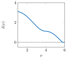
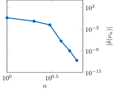
Figure 1. Value function $\delta$ (left) and absolute value of $\delta(\nu_{n})$ (right) for $\nu_{n}$ the iterates generated by the Newton method (Algorithm 1) for Example 7.1 with $M=10\,000$ time steps for the implicit Euler method.

$M$	$T_{k}$	$\lvert T_{k}-T\rvert$	Newton steps	cG steps
$100$	$5.501553$	$2.5803_{-1}$	$6$ ($1$)	$44$
$1\,000$	$5.730029$	$2.9557_{-2}$	$6$ ($1$)	$52$
$10\,000$	$5.756636$	$2.9504_{-3}$	$6$ ($1$)	$58$
$100\,000$	$5.759346$	$2.4051_{-4}$	$6$ ($1$)	$56$
$1\,000\,000$	$5.759618$	$3.1244_{-5}$	$6$ ($1$)	$53$

Table 1. Computed optimal times, absolute errors, number of Newton steps in outer loop (number of damped steps in brackets), and number of conditional gradient steps in inner loop for Example 7.1 with $M$ denoting the number of time steps. Moreover, $\delta_{0}=10^{-6}$ and the inital value for the Newton method is $\nu_{0}=0.6\,T$.

7.2. Linear heat-equation with distributed control

Next, we consider the following problem subject to the linear heat-equation. Let

$$\Omega =(0,1)^{2}\mbox{,}\quad\omega=(0.25,0.75)^{2}\mbox{,}\quad\delta_{0}=1/10,$$

$$y_{0}(x) =4\sin(\pi x_{1}^{2})\sin(\pi x_{2})^{3},\quad y_{d}(x)=-2\min\set{x_{1},1-x_{1},x_{2},1-x_{2}}\mbox{,}$$

$$U_{ad}(0,1) =\set{u\in L^{2}(I\times\omega)\colon-5\leq u\leq 0}\mbox{.}$$

Moreover, $A=-0.03\upDelta$ with $-\upDelta$ the Laplace operator equipped with homogeneous Dirichlet boundary conditions. The control operator $B$ is the extension by zero operator. Hence, we take $V=H^{1}_{0}(\Omega)$, $H=L^{2}(\Omega)$, $V^{*}=H^{-1}(\Omega)$, and $U=L^{2}(\omega)$. Note that the control acts on a subset $\omega\subset\Omega$, only. Concerning the practical implementation, we consider a discontinuous Galerkin method in time and a continuous Galerkin method in space. The state and adjoint state equations are discretized by means of piecewise constant functions in time (corresponding to the implicit Euler method) and continuous and cellwise linear functions in space.

$M$	$N$	$T_{k}$	$\lvert T_{k}-T\rvert$	Newton steps	cG steps
$20$	$4225$	$1.573876$	$9.0814_{-2}$	$6$ ($0$)	$206$
$40$	$4225$	$1.525617$	$4.2554_{-2}$	$6$ ($0$)	$210$
$80$	$4225$	$1.501899$	$1.8836_{-2}$	$6$ ($0$)	$209$
$160$	$4225$	$1.490127$	$7.0645_{-3}$	$6$ ($0$)	$210$
$320$	$4225$	$1.484246$	$1.1830_{-3}$	$6$ ($0$)	$196$
$640$	$81$	$1.291744$	$1.9132_{-1}$	$6$ ($0$)	$133$
$640$	$289$	$1.423571$	$5.9492_{-2}$	$6$ ($0$)	$162$
$640$	$1089$	$1.468758$	$1.4304_{-2}$	$6$ ($0$)	$188$
$640$	$4225$	$1.481302$	$1.7608_{-3}$	$6$ ($0$)	$190$

Table 2. Computed optimal times, absolute errors, number of Newton steps in outer loop (number of damped steps in brackets), and number of conditional gradient steps in inner loop for Example 7.2 with $M$ denoting the number of time steps and $N$ the number of nodes for the spatial discretization. Moreover, the inital value for the Newton method is $\nu_{0}=0.8$.

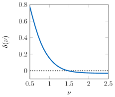
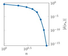
Figure 2. Value function $\delta$ (left) and absolute value of $\delta(\nu_{n})$ (right) for $\nu_{n}$ the iterates generated by the Newton method (Algorithm 1) for Example 7.2.

As in the first example, we observe fast convergence of the Newton method, see Tables 2 and 2. Moreover, we observe quadratic order of convergence with respect to the spatial discretization and linear order convergence with respect to the temporal discretization. For further details and a priori discretization error estimates we also refer to [4].

Before turning to the next example, we would like to compare the algorithm from Section 6 to an alternative approach, where the time-optimal control problem ($\hat{P}$) is solved directly after adding a regularization term to the objective functional, precisely the $L^{2}$-norm of the control variable. Clearly, we are interested in steering the regularization parameter to zero. The terminal constraint in ($\hat{P}$) is treated algorithmically by means of the augmented Lagrange method. The resulting optimization problems are solved by means of a semi-smooth Newton method in a monolithic way, i.e. we consider the tuple $(\nu,u)$ as a joint optimization variable; cf. [18] and [2, Section 4.1]. We observe that our approach requires roughly four to ten times less solves of the PDE than the regularization approach for any fixed regularization parameter in the range from $\alpha=0.001$ to $\alpha=10$; see Table 3. Employing a path-following strategy, where one iteratively decreases the regularization parameter starting with a moderate value of $\alpha$ and uses the solution of the former iteration as the initial value for the next optimization (see, e.g., [14]), one could avoid the high computational costs for small $\alpha$. However, this strategy requires at least one solution without warm start, so that our approach is (in this example) at least five times faster.

		Min. dist.	Augmented Lagrange method with regularization
$M$	$N$		$\alpha=0.001$	$\alpha=0.01$	$\alpha=0.1$	$\alpha=1$	$\alpha=10$
$20$	$4225$	$260$	$2681$	$1598$	$1208$	$1375$	$1813$
$40$	$4225$	$250$	$2703$	$1447$	$1177$	$1440$	$1675$
$80$	$4225$	$250$	$2687$	$1424$	$1130$	$1434$	$1685$
$160$	$4225$	$252$	$3017$	$1697$	$1154$	$1388$	$1705$
$320$	$4225$	$222$	$3068$	$1587$	$1100$	$1356$	$1709$
$640$	$81$	$214$	$1879$	$1091$	$924$	$1074$	$1215$
$640$	$289$	$198$	$1824$	$1070$	$774$	$1180$	$1479$
$640$	$1089$	$212$	$2495$	$1412$	$1028$	$1372$	$1789$
$640$	$4225$	$246$	$3597$	$1647$	$1050$	$1364$	$1781$

Table 3. Number of PDE solves for the algorithm from Section 6 based on solving minimal distance problems and the augmented Lagrange method with $L^{2}$-regularization for the control and $\alpha$ the regularization parameter. $M$ denotes the number of intervals for the temporal discretization and $N$ the number of nodes for the spatial discretization of the PDE. The initial parameters for the augmented Lagrange method are $c_{0}=2\cdot 10^{4}$ and $\mu_{0}=80$.

7.3. Linear heat-equation with Neumann boundary control

Last, we consider the following problem subject to the linear heat-equation with Neumann boundary control. Concretely, let

$$\Omega =(0,1)^{2}\mbox{,}\quad\omega=\partial\Omega\mbox{,}\quad\delta_{0}=1/10,$$

$$y_{0}(x) =4\sin(\pi x_{1}^{2})\sin(\pi x_{2})^{3},\quad y_{d}(x)=0\mbox{,}$$

$$U_{ad}(0,1) =\set{u\in L^{2}(I\times\omega)\colon-5\leq u\leq 5}\mbox{.}$$

Moreover, $A=-0.03\upDelta$ with $-\upDelta$ the Laplace operator. The control operator $B$ is the adjoint of the trace operator, i.e. $B=\mathrm{Tr}^{*}\colon L^{2}(\partial\Omega)\to(H^{1}(\Omega))^{*}$. Hence, we take $V=H^{1}(\Omega)$, $H=L^{2}(\Omega)$, $V^{*}=(H^{1}(\Omega))^{*}$, and $U=L^{2}(\omega)$. We consider the same discretization scheme for the state and adjoint state equation as before. Moreover, the control is discretized by edge-wise constant functions on the boundary.

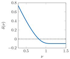
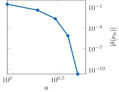
Figure 3. Value function $\delta$ (left) and absolute value of $\delta(\nu_{n})$ (right) for $\nu_{n}$ the iterates generated by the Newton method (Algorithm 1) for Example 7.3.

$M$	$N$	$T_{k}$	$\lvert T_{k}-T\rvert$	Newton steps	cG steps
$20$	$4225$	$8.8971_{-1}$	$4.0493_{-2}$	$4$ ($0$)	$3302$
$40$	$4225$	$8.6784_{-1}$	$1.8619_{-2}$	$4$ ($0$)	$4141$
$80$	$4225$	$8.5681_{-1}$	$7.5882_{-3}$	$4$ ($0$)	$4979$
$160$	$4225$	$8.5134_{-1}$	$2.1231_{-3}$	$4$ ($0$)	$6294$
$320$	$81$	$6.9746_{-1}$	$1.5176_{-1}$	$3$ ($0$)	$1938$
$320$	$289$	$8.1011_{-1}$	$3.9113_{-2}$	$4$ ($0$)	$5265$
$320$	$1089$	$8.4096_{-1}$	$8.2584_{-3}$	$4$ ($0$)	$8029$
$320$	$4225$	$8.4865_{-1}$	$5.7155_{-4}$	$4$ ($0$)	$8432$

Table 4. Computed optimal times, absolute errors, number of Newton steps in outer loop (number of damped steps in brackets), and number of conditional gradient steps in inner loop for Example 7.3 with $M$ denoting the number of time steps and $N$ the number of nodes for the spatial discretization. Moreover, the initial value for the Newton method is $\nu_{0}=0.6$.

The optimal control obtained numerically is depicted in Figure 4, where the boundary of the square domain has been unrolled. Note that switching hyperplanes of the control seem to accumulate towards the end of the time horizon. As in the preceding examples, we observe fast convergence of the Newton method for the outer loop; see Figures 3 and 4.

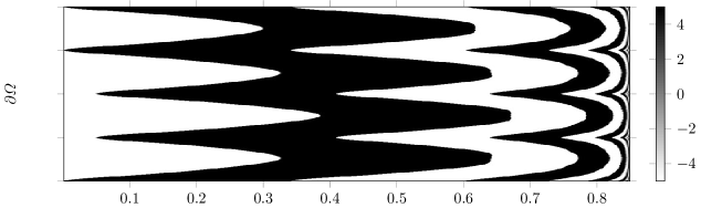
Figure 4. Optimal control for Example 7.3. Black denotes the upper bound and white the lower bound of the control constraints.

8. Open problems

We conclude with some open problems.

1. To prove the equivalence of time-optimal and distance-optimal controls, we required that $T(\cdot)$ is left-continuous; see Theorem 3.1. We stated two sufficient conditions; see Propositions 3.5 and 3.6. The latter can be checked a priori without knowing an optimal solution, whereas the first depends on a certain controllability condition under pointwise control constraints that is difficult to verify. It would be desirable to know further sufficient conditions that can be easily verified for concrete problems.

2. Moreover, to strengthen the directional derivative of $\delta(\cdot)$ to a classical derivative, one has to ensure that the integral expression in (5.7) is independent of the control variable. This is guaranteed for purely time-dependent controls (see Proposition 5.7) or if a backwards uniqueness property holds (see Corollary 5.6). Clearly, the backwards uniqueness property of other control scenarios is of independent interest and would also lead to more applications for our approach.

3. Last, Lipschitz continuity of $\delta^{\prime}(\cdot)$ yields fast local convergence of the Newton method, which further justifies to use the equivalence of time-optimal and distance-optimal controls for numerical realization. Here, we only stated one sufficient condition that relies on the structural assumption of the adjoint state (5.12); see Proposition 6.4. This condition does not seem to be sufficient as we observe Lipschitz continuity of $\delta^{\prime}(\cdot)$ in the numerical examples even if (5.12) is violated. Different techniques to show Lipschitz continuity of $\delta^{\prime}(\cdot)$ would require a second order sufficient optimality condition. However, such a condition cannot be expected to hold in the case of bang-bang controls.

References

• [1] H. Amann and J. Escher. Analysis. I. Birkhäuser Verlag, Basel, 2005. Translated from the 1998 German original by Gary Brookfield.
• [2] L. Bonifacius. Numerical Analysis of Parabolic Time-optimal Control Problems. PhD thesis, Technische Universität München, 2018.
• [3] L. Bonifacius and K. Pieper. Strong stability of linear parabolic time-optimal control problems. ESAIM: Control, Optimisation and Calculus of Variations, 2019.
• [4] L. Bonifacius, K. Pieper, and B. Vexler. Error estimates for space-time discretization of parabolic time-optimal control problems with bang-bang controls. SIAM J. Control Optim. Accepted.
• [5] E. Casas, D. Wachsmuth, and G. Wachsmuth. Sufficient Second-Order Conditions for Bang-Bang Control Problems. SIAM J. Control Optim., 55(5):3066–3090, 2017.
• [6] R. Dautray and J.-L. Lions. Mathematical analysis and numerical methods for science and technology. Vol. 5. Springer-Verlag, Berlin, 1992. Evolution problems. I, With the collaboration of Michel Artola, Michel Cessenat and Hélène Lanchon, Translated from the French by Alan Craig.
• [7] J. C. Dunn. Convergence rates for conditional gradient sequences generated by implicit step length rules. SIAM J. Control Optim., 18(5):473–487, 1980.
• [8] H. O. Fattorini. Infinite dimensional linear control systems, volume 201 of North-Holland Mathematics Studies. Elsevier Science B.V., Amsterdam, 2005. The time optimal and norm optimal problems.
• [9] R. Glowinski, J.-L. Lions, and J. He. Exact and approximate controllability for distributed parameter systems, volume 117 of Encyclopedia of Mathematics and its Applications. Cambridge University Press, Cambridge, 2008. A numerical approach.
• [10] F. Gozzi and P. Loreti. Regularity of the minimum time function and minimum energy problems: the linear case. SIAM J. Control Optim., 37(4):1195–1221, 1999.
• [11] M. Gugat. A Newton method for the computation of time-optimal boundary controls of one-dimensional vibrating systems. J. Comput. Appl. Math., 114(1):103–119, 2000. Control of partial differential equations (Jacksonville, FL, 1998).
• [12] Q. Han and F.-H. Lin. Nodal sets of solutions of parabolic equations. II. Comm. Pure Appl. Math., 47(9):1219–1238, 1994.
• [13] H. Hermes and J. P. LaSalle. Functional analysis and time optimal control. Academic Press, New York-London, 1969. Mathematics in Science and Engineering, Vol. 56.
• [14] M. Hintermüller and K. Kunisch. Path-following methods for a class of constrained minimization problems in function space. SIAM J. Optim., 17(1):159–187, 2006.
• [15] K. Ito and K. Kunisch. Semismooth Newton methods for time-optimal control for a class of ODEs. SIAM J. Control Optim., 48(6):3997–4013, 2010.
• [16] C. Y. Kaya and J. L. Noakes. Computational method for time-optimal switching control. J. Optim. Theory Appl., 117(1):69–92, 2003.
• [17] W. Krabs. Optimal control of processes governed by partial differential equations. I. Heating processes. Z. Oper. Res. Ser. A-B, 26(1):A21–A48, 1982.
• [18] K. Kunisch, K. Pieper, and A. Rund. Time optimal control for a reaction diffusion system arising in cardiac electrophysiology - a monolithic approach. ESAIM: Mathematical Modelling and Numerical Analysis, 2016.
• [19] K. Kunisch and D. Wachsmuth. On time optimal control of the wave equation, its regularization and optimality system. ESAIM Control Optim. Calc. Var., 19(2):317–336, 2013.
• [20] X. J. Li and J. M. Yong. Optimal control theory for infinite-dimensional systems. Systems & Control: Foundations & Applications. Birkhäuser Boston, Inc., Boston, MA, 1995.
• [21] X. Lu, L. Wang, and Q. Yan. Computation of time optimal control problems governed by linear ordinary differential equations. J. Sci. Comput., 73(1):1–25, 2017.
• [22] J. W. Macki and A. Strauss. Introduction to optimal control theory. Springer-Verlag, New York-Berlin, 1982. Undergraduate Texts in Mathematics.
• [23] E.-B. Meier and A. E. Bryson, Jr. Efficient algorithm for time-optimal control of a two-link manipulator. J. Guidance Control Dynam., 13(5):859–866, 1990.
• [24] A. Münch and F. Periago. Numerical approximation of bang-bang controls for the heat equation: an optimal design approach. Systems Control Lett., 62(8):643–655, 2013.
• [25] A. Münch and E. Zuazua. Numerical approximation of null controls for the heat equation: ill-posedness and remedies. Inverse Problems, 26(8):085018, 39, 2010.
• [26] J. Nocedal and S. J. Wright. Numerical optimization. Springer Series in Operations Research and Financial Engineering. Springer, New York, second edition, 2006.
• [27] E. M. Ouhabaz. Analysis of heat equations on domains, volume 31 of London Mathematical Society Monographs Series. Princeton University Press, Princeton, NJ, 2005.
• [28] A. Pazy. Semigroups of linear operators and applications to partial differential equations, volume 44 of Applied Mathematical Sciences. Springer-Verlag, New York, 1983.
• [29] K. Pieper. Finite element discretization and efficient numerical solution of elliptic and parabolic sparse control problems. PhD thesis, Technische Universität München, 2015.
• [30] S. Qin and G. Wang. Equivalence between Minimal Time and Minimal Norm Control Problems for the Heat Equation. SIAM J. Control Optim., 56(2):981–1010, 2018.
• [31] S. M. Robinson. Normal maps induced by linear transformations. Math. Oper. Res., 17(3):691–714, 1992.
• [32] F. Tröltzsch. Optimal control of partial differential equations, volume 112 of Graduate Studies in Mathematics. American Mathematical Society, Providence, RI, 2010. Theory, methods and applications, Translated from the 2005 German original by Jürgen Sprekels.
• [33] M. Tucsnak and G. Weiss. Observation and control for operator semigroups. Birkhäuser Advanced Texts: Basler Lehrbücher. [Birkhäuser Advanced Texts: Basel Textbooks]. Birkhäuser Verlag, Basel, 2009.
• [34] G. Wang, L. Wang, Y. Xu, and Y. Zhang. Time Optimal Control of Evolution Equations. Progress in Nonlinear Differential Equations and Their Applications. Springer International Publishing, 2018.
• [35] G. Wang and Y. Xu. Equivalence of three different kinds of optimal control problems for heat equations and its applications. SIAM J. Control Optim., 51(2):848–880, 2013.
• [36] G. Wang and E. Zuazua. On the equivalence of minimal time and minimal norm controls for internally controlled heat equations. SIAM J. Control Optim., 50(5):2938–2958, 2012.
• [37] W. Wang and M. Á. Carreira-Perpiñán. Projection onto the probability simplex: An efficient algorithm with a simple proof, and an application. ArXiv e-prints, Sept. 2013.
• [38] C. Zhang. The time optimal control with constraints of the rectangular type for linear time-varying ODEs. SIAM J. Control Optim., 51(2):1528–1542, 2013.
• [39] Y. Zhang. Two equivalence theorems of different kinds of optimal control problems for Schrödinger equations. SIAM J. Control Optim., 53(2):926–947, 2015.