Graph-based algorithms for the efficient solution of a class of optimization problems

Abstract

In this paper, we address a class of specially structured problems that include speed planning, for mobile robots and robotic manipulators, and dynamic programming. We develop two new numerical procedures, that apply to the general case and to the linear subcase. With numerical experiments, we show that the proposed algorithms outperform generic commercial solvers.

Index terms— Computational methods, Acceleration of convergence, Dynamic programming, Complete lattices

1 Introduction

In this paper, we address a class of specially structured problems of form

$$\max_{x}f(x)$$ (1)

subject to $$a\leq x\leq g(x),$$

where $x\in\mathbb{R}^{n}$, $a\in\mathbb{R}^{n}$, $f:\mathbb{R}^{n}\rightarrow\mathbb{R}$ is a continuous function, strictly monotone increasing with respect to each component and $g=(g_{1},g_{2},\ldots,g_{n})^{T}:\mathbb{R}^{n}\rightarrow\mathbb{R}^{n}$, is a continuous function such that, for $i=1,\ldots,n$, $g_{i}$ is monotone not decreasing with respect to all variables and constant with respect to $x_{i}$. Also, we assume that there exists a real constant vector $U$ such that

$$g(x)\leq U,\forall x:a\leq x\leq g(x)\,.$$ (2)

A Problem related to (1) that is relevant in applications is the following one

$$\max_{x}f(x)$$ (3)

subject to $$0\leq x\leq\underset{\ell\in\mathcal{L}}{\operatorname{\bigwedge}}\left\{A_{\ell}x+b_{\ell}\right\},\ x\leq U,$$

where, for each $\ell\in\mathcal{L}=\{1,\ldots,L\}$, with $L\in\mathbb{N}$, $A_{\ell}$ is a nonnegative matrix and $b_{\ell}$ is a nonnegative vector.

Note that the expression $\underset{\ell\in\mathcal{L}}{\operatorname{\bigwedge}}$, on the right hand side of (3), denotes the greatest lower bound of $L$ vectors. It corresponds to the component-wise minimum of vectors $A_{\ell}x+b_{\ell}$, where a different value of $\ell\in\mathcal{L}$ can be chosen for each component. We will show that Problem (3) is actually a subclass of (1) after a suitable definition of function $g$ in (1).

We will also show that the solution of Problems (1) and (3) is independent on the specific choice of $f$. Hence, Problem (3) is equivalent to the following linear one

$$\max_{x}\sum_{i=1}^{n}x_{i}$$ (4)

subject to $$0\leq x,Cx+d\leq 0,x\leq U,$$

where $C$ is a matrix such that every row contains one and only one positive entry and $d$ is a nonpositive vector.

The structure of the paper is the following: in Section 1.1 we justify the interest in Problem class (1) and, in particular, its subclass (3), by presenting some problems in control, which can be reformulated as optimization problems within subclass (3). In Section 2 we derive some theoretical results about Problem (1) and a class of algorithms for its solution. In Section 3 we do the same for the subclass (3). In Section 4 we discuss some theoretical and practical issues about convergence speed of the algorithms and we present some numerical experiments. Some proofs are given in the appendix.

1.1 Problems reducible to form (3)

1.1.1 Speed planning for autonomous vehicles

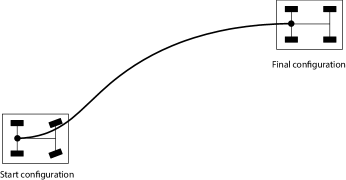
Figure 1: A path to follow for an autonomous car-like vehicle.

This example is taken from [8] and we refer the reader to this reference for further detail. We consider a speed planning problem for a mobile vehicle (see Figure 1). We assume that the path that joins the initial and the final configuration is assigned and we aim at finding the time-optimal speed law that satisfies some kinematic and dynamic constraints. Namely, we consider the following problem

$$\min_{v\in C^{1}([0,s_{f}],\mathbb{R})}\int_{0}^{s_{f}}v^{-1}(s)ds$$ (5a)

subject to $$v(0)=0,\,v(s_{f})=0$$ (5b)

$$0<v(s)\leq\bar{v}, s\in(0,s_{f}),$$ (5c)

$$|2v^{\prime}(s)v(s)|\leq A_{T}, s\in[0,s_{f}],$$ (5d)

$$|k(s)|v(s)^{2}\leq A_{N}, s\in[0,s_{f}],$$ (5e)

where $\bar{v}$, $A_{T}$, $A_{N}$ are upper bounds for the velocity, the tangential acceleration and the normal acceleration, respectively. Here, $s_{f}$ is the length of the path (that is assumed to be parameterized according to its arc length) and $k$ is its scalar curvature (i.e., a function whose absolute value is the inverse of the radius of the circle that locally approximates the trajectory).

The objective function (5a) is the total maneuver time, constraints (5b) are the initial and final interpolation conditions and constraints (5c), (5d), (5e) limit velocity and tangential and normal components of acceleration.

After the change of variable $w=v^{2}$, the problem can be rewritten as

$$\min_{w\in C^{1}([0,s_{f}],\mathbb{R})}\int_{0}^{s_{f}}w(s)^{-1/2}ds$$ (6a)

subject to $$w(0)=0,\,w(s_{f})=0,$$ (6b)

$$0<w(s)\leq\bar{v}^{2}, s\in(0,s_{f}),$$ (6c)

$$|w^{\prime}(s)|\leq A_{T}, s\in[0,s_{f}],$$ (6d)

$$|k(s)|w(s)\leq A_{N}, s\in[0,s_{f}].$$ (6e)

For $i=1\,\ldots,n$, set $w_{i}=w((i-1)h)$, with $h=\frac{s_{f}}{n-1}$, then Problem (6) can be approximated with

$$\min_{w\in\mathbb{R}^{n}}\ \ \phi(w)$$ (7a)

subject to $$w_{1}=0,\,w_{n}=0,$$ (7b)

$$0<w_{i}\leq\bar{v}^{2}, i=2,\ldots,n-1,$$ (7c)

$$|w_{i+1}-w_{i}|\leq hA_{T}, i=1,\ldots,n-1,$$ (7d)

$$|k(h(i-1))|w_{i}\leq A_{N}, i=2,\ldots,n-1,$$ (7e)

where the total time to travel the complete path is approximated by

$$\phi(w)=\sum_{i=1}^{n-1}t_{i}=2h\sum_{i=1}^{n-1}\frac{1}{\sqrt{w_{i}}+\sqrt{w_{i+1}}}.$$ (8)

Note that conditions (7d) is obtained by Euler approximation of $w^{\prime}(hi)$. Similarly, the objective function (8) is a discrete approximation of the integral appearing in (6a). By setting $f(w)=\phi(w)$, $a=0$, $g_{1}(w)=0$, $g_{n}(w)=0$ and, for $i=2,\ldots,n-1$,

$$g_{i}(w)=\bigwedge\left\{\bar{v}^{2},\frac{A_{N}}{|k(h(i-1))|},hA_{T}+w_{i-1},hA_{T}+w_{i+1}\right\}\,,$$

Problem (7) takes on the form of Problem (1) and, since $g$ is linear with respect to $w$, it also belongs to the more specific class (3). We remark that, with respect to the problem class (3), we minimize a decreasing function which is equivalent to maximizing an increasing function.

Our previous works [7], [8] present an algorithm, with linear-time computational complexity with respect to the number of variables $n$, that provides an optimal solution of Problem (7). This algorithm is a specialization of the algorithms proposed in this paper which exploits some specific feature of Problem (7). In particular, the key property of Problem (7), which strongly simplifies its solution, is that functions $g_{i}$ fulfill the so-called superiority condition

$$g_{i}(w_{i-1},w_{i+1})\geq w_{i-1},w_{i+1},$$

i.e., the value of function $g_{i}$ is not lower than each one of its arguments.

1.1.2 Speed planning for robotic manipulators

The technical details of this second example are more involved and we refer the reader to [6] for the complete discussion. Let $\mathbb{R}^{p}$ be the configuration space of a robotic manipulator with $p$-degrees of freedom. The coordinate vector $\mathbf{q}$ of a trajectory in $U$ satisfies the dynamic equation

$$\boldsymbol{D}(\mathbf{q})\ddot{\mathbf{q}}+\boldsymbol{C}(\mathbf{q},\dot{\mathbf{q}})\dot{\mathbf{q}}+\boldsymbol{\ell}(\mathbf{q})=\boldsymbol{\tau},$$ (9)

where $\mathbf{q}\in\mathbb{R}^{p}$ is the generalized position vector, $\boldsymbol{\tau}\in\mathbb{R}^{p}$ is the generalized force vector, $\boldsymbol{D}(\mathbf{q})$ is the mass matrix, $\boldsymbol{C}(\mathbf{q},\dot{\mathbf{q}})$ is the matrix accounting for centrifugal and Coriolis effects (assumed to be linear in $\dot{\mathbf{q}}$) and $\boldsymbol{\ell}(\mathbf{q})$ is the vector accounting for joints position dependent forces, including gravity. Note that we do not consider Coulomb friction forces.

Let $\boldsymbol{\gamma}\in C^{2}([0,s_{f}],\mathbb{R}^{p})$ be a function such that ($\forall\lambda\in[0,s_{f}]$) $\lVert\boldsymbol{\gamma}^{\prime}(\lambda)\rVert=1$. The image set $\boldsymbol{\gamma}([0,s_{f}])$ represents the coordinates of the elements of a reference path. In particular, $\boldsymbol{\gamma}(0)$ and $\boldsymbol{\gamma}(s_{f})$ are the coordinates of the initial and final configurations. Define $t_{f}$ as the time when the robot reaches the end of the path. Let $\lambda:[0,t_{f}]\rightarrow[0,s_{f}]$ be a differentiable monotone increasing function that represents the position of the robot as a function of time and let $v:[0,s_{f}]\rightarrow[0,+\infty]$ be such that $\left(\forall t\in[0,t_{f}]\right)\dot{\lambda}(t)=v(\lambda(t))$. Namely, $v(s)$ is the velocity of the robot at position $s$. We impose ($\forall s\in[0,s_{f}]$) $v(s)\geq 0$. For any $t\in[0,t_{f}]$, using the chain rule, we obtain

$$\begin{array}[]{ll}\mathbf{q}(t)=&\boldsymbol{\gamma}(\lambda(t)),\\[8.0pt] \dot{\mathbf{q}}(t)=&\boldsymbol{\gamma}^{\prime}(\lambda(t))v(\lambda(t)),\\[8.0pt] \ddot{\mathbf{q}}(t)=&\boldsymbol{\gamma}^{\prime}(\lambda(t))v^{\prime}(\lambda(t))v(\lambda(t))+\boldsymbol{\gamma}^{\prime\prime}(\lambda(t))v(\lambda(t))^{2}.\end{array}$$ (10)

Substituting (10) into the dynamic equations (9) and setting $s=\lambda(t)$, we rewrite the dynamic equation (9) as follows:

$$\mathbf{d}(s)v^{\prime}(s)v(s)+\mathbf{c}(s)v(s)^{2}+\mathbf{g}(s)=\boldsymbol{\tau}(s),$$ (11)

where the parameters in (11) are defined as

$$\begin{array}[]{l}\mathbf{d}(s)=\boldsymbol{D}(\boldsymbol{\gamma}(s))\boldsymbol{\gamma}^{\prime}(s),\\[8.0pt] \mathbf{c}(s)=\boldsymbol{D}(\boldsymbol{\gamma}(s))\boldsymbol{\gamma}^{\prime\prime}(s)+\boldsymbol{C}(\boldsymbol{\gamma}(s),\boldsymbol{\gamma}^{\prime}(s))\boldsymbol{\gamma}^{\prime}(s),\\[8.0pt] \mathbf{g}(s)=\boldsymbol{\ell}(\boldsymbol{\gamma}(s)).\end{array}$$ (12)

The objective function is given by the overall travel time $t_{f}$ defined as

$$t_{f}=\int_{0}^{t_{f}}1\,dt=\int_{0}^{s_{f}}v(s)^{-1}\,ds.$$ (13)

Let $\boldsymbol{\mu},\boldsymbol{\psi},\boldsymbol{\alpha}:\left[0,s_{f}\right]\rightarrow\mathbb{R}^{p}_{+}$ be assigned bounded functions and consider the following minimum time problem:

$$\displaystyle\min_{v\in C^{1},\boldsymbol{\tau}\in C^{0}}\displaystyle\int_{0}^{s_{f}}v(s)^{-1}\,ds,$$ (14a)

subject to $$\ (\forall s\in[0,s_{f}])$$

$$\mathbf{d}(s)v^{\prime}(s)v(s)+\mathbf{c}(s)v(s)^{2}+\mathbf{g}(s)=\boldsymbol{\tau}(s),$$ (14b)

$$\boldsymbol{\gamma}^{\prime}(s)v(s)=\dot{\mathbf{q}}(s),$$ (14c)

$$\boldsymbol{\gamma}^{\prime}(s)v^{\prime}(s)v(s)+\boldsymbol{\gamma}^{\prime\prime}(s)v(s)^{2}=\ddot{\mathbf{q}}(s),$$ (14d)

$$\lvert\boldsymbol{\tau}(s)\rvert\leq\boldsymbol{\mu}(s),$$ (14e)

$$\lvert\dot{\mathbf{q}}(s)\rvert\leq\boldsymbol{\psi}(s),$$ (14f)

$$\lvert\ddot{\mathbf{q}}(s)\rvert\leq\boldsymbol{\alpha}(s),$$ (14g)

$$v(s)\geq 0,$$ (14h)

$$v(0)=0,\,v(s_{f})=0,$$ (14i)

where (14b) represents the robot dynamics, (14c)-(14d) represent the relation between the path $\boldsymbol{\gamma}$ and the generalized position $\mathbf{q}$ shown in (10), (14e) represents the bounds on generalized forces, (14f) and (14g) represent the bounds on joints velocity and acceleration, respectively. Constraints (14i) specify the interpolation conditions at the beginning and at the end of the path.

After some manipulation and using a carefully chosen finite dimensional approximation (again, see [6] for the details), Problem (14) can be reduced to form (see Proposition 8 of [6]).

$$\min_{w}\phi(w)$$ (15)

subject to $$w_{i}\leq f_{j,i}w_{i+1}+c_{j,i} i=1,\ldots,n-1,\quad j=1,\ldots,p,$$

$$w_{i+1}\leq b_{k,i}w_{i}+d_{k,i} i=1,\ldots,n-1,\quad k=1,\ldots,p,$$

$$0\leq w_{i}\leq u_{i} i=1,\ldots,n,$$

where, $\phi$ is defined as in (8) and $w=(w_{1},\ldots,w_{n})^{T}$. For $i=1,\ldots,n$, $w_{i}=v((i-1)h)^{2}$, $h=\frac{s_{f}}{n-1}$, is the squared manipulator speed at configuration $\boldsymbol{\gamma}((i-1)h)$. Moreover $u_{i}$, $f_{j,i}$, $c_{j,i}$, $b_{k,i}$, $d_{k,i}$ are nonnegative constant terms depending on problem data.

Problem (15) belongs to classes (1) and (3). Also in this case, the performance of the algorithms proposed in this paper can be enhanced by exploiting some further specific features of Problem (15). In particular, in [6], we were able to develop a version of the algorithm with optimal time-complexity $O(np)$.

1.1.3 Dynamic Programming

This section is based on Appendix A of [3], to which we refer the reader for more detail. Consider a control system defined by the following differential equation in $\mathbb{R}^{n}$:

$$\begin{cases}\dot{x}(t)=f(x(t),u(t))\\ x(0)=x_{0},\end{cases}$$ (16)

where $f:\mathbb{R}^{n}\times U\rightarrow\mathbb{R}^{n}$ is a continuous function, $x_{0}$ is the initial state, $u(t)\in U\subset\mathbb{R}^{m}$ is the control input and $U$ is a compact set of admissible controls. Consider an infinite horizon cost functional defined as follows

$$J_{x_{0}}(u)=\int\limits_{0}^{\infty}g(x(t),u(t))e^{-\lambda t}dt,$$ (17)

where $g:\mathbb{R}^{n}\times U\rightarrow\mathbb{R}$ is a continuous cost function. The viscosity parameter $\lambda$ is a positive real constant. Following [3], we assume that there exist positive real constants $L_{f}$, $L_{g}$, $C_{f}$, $C_{g}$ such that, $\forall x_{1},x_{2}\in\mathbb{R}^{n}$, $\forall u\in U$,

$$|f(x_{1},u)-f(x_{2},u)|\leq L_{f}|x_{1}-x_{2}|,\qquad \left\|f(x_{1},u)\right\|_{\infty}\leq C_{f},$$

$$|g(x_{1},u)-g(x_{2},u)|\leq L_{g}|x_{1}-x_{2}|,\qquad \left\|g(x_{1},u)\right\|_{\infty}\leq C_{g}.$$

Define the value function $v:\mathbb{R}^{n}\to\mathbb{R}$ as

$$v(x_{0})=\inf_{u\in U}J_{x_{0}}(u).$$

As shown in [3], the value function $v$ is the unique viscosity solution of the Hamilton-Jacobi-Bellman (HJB) equation:

$$\lambda v(x)+\sup_{u\in U}\{-\nabla v(x)f(x,u)-g(x,u)\}=0,\quad x\in\mathbb{R}^{n},$$ (18)

where $\nabla v$ denotes the gradient of $v$.

In general, a closed form solution of the partial differential equation (18) does not exist. Various numerical procedures have been developed to compute approximate solutions, such as in [1], [3] [13], [15].

In particular, [3] presents an approximation scheme based on a finite approximation of state and control spaces and a discretization in time. Roughly speaking, in (18) one can approximate $\nabla v(x)f(x,u)\simeq h^{-1}(v(x+hf(x,u))-v(x))$, where $h$ is a small positive real number that represents an integration time. In this way, (18) becomes

$$(1+\lambda h)v(x)=\min_{u\in U}\{v(x+hf(x,u))+hg(x,u)\}=0,\ x\in\mathbb{R}^{n},$$

and, by approximating $(1+\lambda h)^{-1}\simeq(1-\lambda h)$, $(1+\lambda h)^{-1}h\simeq h$, one arrives at the following HJB equation in discrete time

$$v_{h}(x)=\min_{u\in U}\left\{(1-\lambda h)v_{h}(x+hf(x,u))+hg(x,u)\right\},\ x\in\mathbb{R}^{n}.$$ (19)

For a more rigorous derivation of (19), again, see [3].

A triangulation is computed on a finite set of vertices $\mathcal{T}=\{x_{i}\}_{i\in\mathcal{V}}\subset\mathbb{R}^{n}$, with $\mathcal{V}\subseteq\mathbb{N}$ and $|\mathcal{V}|=N$. Evaluating (19) at $x\in\mathcal{T}$, we obtain

$$v_{h}(x_{i})=\min_{u\in U}\left\{(1-\lambda h)v_{h}(x_{i}+hf(x_{i},u))+hg(x_{i},u)\right\},\ i\in\mathcal{V}.$$ (20)

Note the dependence of the value cost function on the choice of the integration step $h$. Using the triangulation, function $v$ can be approximated by a linear affine function of the finite set of variables $v_{h}(x_{i})$, with $i\in\{1,\ldots,N\}$.

Theorem 2.1 of Appendix A of [3] shows that, if $\lambda>L_{f}$ and $h\in\left(\left.0,\frac{1}{\lambda}\right]\right.$, system (20) has a unique solution that converges uniformly to the solution of (18) as $h,d,\frac{d}{h}$ tend to $0$, where $d$ is the maximum diameter of the simplices used in the triangulation. Note that, for convergence results, one should choose $\lambda$ large enough since it is bounded from below by $L_{f}$.

To further simplify (20), it is possible to discretize the control space, substituting $U$ with a finite set of controls $\{u_{\ell}\}_{\ell\ \in\mathcal{L}}$, so that we can replace (20) with

$$v_{h}(x_{i})=\min_{\ell\in\mathcal{L}}\left\{(1-\lambda h)v_{h}(x_{i}+hf(x_{i},u_{\ell}))+hg(x_{i},u_{\ell})\right\},\ i\in\mathcal{V}.$$ (21)

Figure 2 illustrates a step of construction of problem (21). Namely, for each node of the triangulation $x_{i}$ and each value of the control $u_{\ell}$, all end points $x_{i}+hf(x_{i},u_{\ell})$ of the Euler approximation of the solution of (16) from the initial state $x_{i}$ are computed. The value cost function for these end points is given by a convex combination of its values on the triangulation vertices.

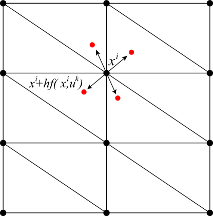
Figure 2: Approximation of the HJB equation on a triangulation with four controls.

Set vector $w:=[w_{1},\ldots,v_{n}]^{T}={[v_{h}(x_{1}),v_{h}(x_{2}),\ldots,v_{h}(x_{N})]}^{T}$, in this way $w\in\mathbb{R}^{N}$ represents the value of the cost function on the grid points.

Note that, for each $x_{i},u_{\ell}$, the right-hand side of (21) is affine with respect to $w$, so that Problem (21) can be rewritten in form

$$\max_{w}\sum_{i}w_{i}$$

subject to $$0\leq w\leq\underset{\ell\in\mathcal{L}}{\operatorname{\bigwedge}}\left\{A_{\ell}w+b_{\ell}\right\},\ w\leq\frac{1}{\lambda}\,,$$

where for $\ell\in\mathcal{L}$, $A_{\ell}\in\mathbb{R}^{N\times N}$ are suitable nonnegative matrices and $b_{\ell}\in\mathbb{R}^{N}$ are suitable nonnegative vectors. Hence, Problem (21) belongs to class (3). Moreover, observe that if $h$ is sufficiently small, matrices ${\left\{A_{\ell}\right\}}_{\ell\in\mathcal{L}}$ are dominant diagonal.

1.2 Statement of Contribution

The main contributions of the paper are the following ones:

• We develop a new procedure (Algorithm 2) for the solution of Problem (1) and a more specific one (Algorithm 3) for its subclass (3). We prove the correctness of these solution methods.

• With numerical experiments, we show that the proposed algorithms outperform generic commercial solvers in the solution of linear problem (3).

1.3 Notation

The set of nonnegative real numbers is denoted by $\mathbb{R}_{+}:=[0,+\infty)$ and $\underline{0}$ denotes the zero vector of $\mathbb{R}^{n}$.

Given $n,m\in\mathbb{N}$, let $x\in\mathbb{R}^{n}$ and $A\in\mathbb{R}^{n\times m}$, for $i\in\{1,\ldots,n\}$, we denote the $i$-th component of $x$ with ${[x]}_{i}$ and the $i$-th row of $A$ with ${[A]}_{i*}$; further, for $j\in\{1,\ldots,m\}$ we denote the $j$-th column of $A$ with ${[A]}_{*j}$ and the $ij$-th element of $A$ with ${[A]}_{ij}$.

Function $\left\|\cdot\right\|_{\infty}:\mathbb{R}^{n}\rightarrow\mathbb{R}_{+}$ is the infinity norm, namely the maximum norm, of $\mathbb{R}^{n}$ (i.e., $\forall\ x\in\mathbb{R}^{n}\ \left\|x\right\|_{\infty}=\max\limits_{i\in\{1,\ldots,n\}}{|{[x]}_{i}|}$); $\left\|\cdot\right\|_{\infty}$ is also used to denote the induced matrix norm. Given a finite set $S$, the cardinality of $S$ is denoted by $|S|$, the power set of $S$ is denoted by $\wp(S)$ and symbol $\varnothing$ denotes the empty set.

Consider the binary relation $\leq$ defined on $\mathbb{R}^{n}$ as follows

$$\forall x,y\in\mathbb{R}^{n}\ (x\leq y\ \Longleftrightarrow\ y-x\in\mathbb{R}_{+}^{n}).$$

It is easy to verify that $\leq$ is a partial order of $\mathbb{R}^{n}$.

Finally, given a nonempty set $\mathcal{V}$ let us define a priority queue $Q$ as a finite subset of $\mathcal{Q}:=\mathcal{V}\times\mathbb{R}$ such that, if $(v,q)\in Q$, then, no other element $(\bar{v},\bar{q})\in Q$ can satisfy that $\bar{v}=v$. Let us also define two operations on priority queues: $\text{Enqueue}:\wp(\mathcal{Q})\times\mathcal{Q}\rightarrow\mathcal{Q}$, which, given $Q\in\wp(\mathcal{Q})$ and $(v,q)\in\mathcal{Q}$, if $Q$ does not contain elements of the form $(v,p)$, with $p\geq q$, then Enqueue adds $(v,q)$ to the priority queue $Q$ and removes any other element of the form $(v,p)$, with $p<q$, if previously present. The second operation we need on priority queues is $\text{Dequeue}:\wp(\mathcal{Q})\rightarrow\wp(\mathcal{Q})\times\mathcal{V}$ which extracts from a priority queue $Q$ the pair $(v,q)$ with highest priority (i.e., it extracts $(v,q)\in Q$ such that $\forall(\bar{v},\bar{q})\in Q,q\geq\bar{q}$) and returns element $v$.

2 Characterization of Problem (1)

In this section, we consider Problem (1) with the additional assumption $g(a)\geq a$ which guarantees that the feasible set of Problem (1)

$$\Sigma=\{x\in\mathbb{R}^{n}:a\leq x\leq g(x)\}\,$$

is non-empty.

For any $\Gamma\subset\Sigma$ define $\bigvee\Gamma$ as the smallest $x\in\Sigma$, if it exists, such that $(\forall y\in\Gamma)\,x\geq y$. We call $\bigvee\Gamma$ the least upper bound of $\Gamma$. Note that $\bigvee\varnothing=a$. The following proposition shows that $\bigvee\Gamma$ exists.

Proposition 2.1.

For any $\Gamma\subset\Sigma$, $\bigvee\Gamma$ exists.

Proof.

We first prove that, if $x,y\in\Sigma$, then $x\vee y\in\Sigma$ (recall that $\vee$ denotes the component-wise maximum). It is obvious that $x\vee y\geq a$. Thus, we only need to prove that, for each $j=1,\ldots,n$, $[y\vee x]_{j}\leq g_{j}(x\vee y)$. To see this, let us assume, w. l. o. g. , that $[x]_{j}\leq[y]_{j}$. Since $y\in\Sigma$, then $[y]_{j}\leq g_{j}(y)$. Moreover, $g_{j}(y)\leq g_{j}(y\vee x)$ since $g_{j}$ is monotone non decreasing, so that $[y\vee x]_{j}\leq g_{j}(y\vee x)$ as we wanted to prove.

Set $\Sigma$ is closed since it is defined by non strict inequalities of a continuous function, $\Sigma$ is bounded by assumption, hence $\Sigma$ is compact. Set $x^{+}=\bigvee\Sigma$, note that $x^{+}\leq U$ since $(\forall x\in\Sigma)x\leq U$, where $U$ is defined in (2). There exists a sequence $x:\mathbb{N}\to\Sigma$ such that $\lim_{k\to\infty}x(k)=x^{+}$. Namely, for any $k>0$, choose $x^{(1)}_{k},\ldots,x^{(n)}_{k}\in\Sigma$ such that $[x^{+}-x^{(i)}_{k}]_{i}<k^{-1}$ and set $x(k)=\bigvee\{x^{(1)}_{k},\ldots,x^{(n)}_{k}\}$. Being $\Sigma$ compact, $\Sigma$ is also sequentially compact and $x^{+}\in\Sigma$. ∎

Similarly, define $\bigwedge\Gamma$ as the largest $x$, if it exists, such that $(\forall y\in\Gamma)x\leq y$, we call $\bigwedge\Gamma$ the greatest lower bound of $\Gamma$.

For $x,y\in\Sigma$, note that $x\vee y=\bigvee\{x,y\}$, $x\wedge y=\bigwedge\{x,y\}$.

The following proposition characterizes set $\Sigma$ with respect to operations $\vee$, $\wedge$. In particular, it shows that the component-wise minimum and maximum of each subset of $\Sigma$ belongs to $\Sigma$.

Proposition 2.2.

Set $\Sigma$ with operations $\vee,\wedge$ defined above is a complete lattice.

Proof.

It is a consequence of the dual of Theorem 2.31 of [9]. Indeed $\Sigma$ has a bottom element ($a$) and $\bigvee\Gamma$ exists for any non-empty $\Gamma\subset\Sigma$ by Proposition 2.1. ∎

A consequence of the previous definition is that also $\bigwedge\Gamma$ exists.

The following proposition shows that the least upper bound $x^{+}$ of $\Sigma$ is a fixed point of $g$ and corresponds to an optimal solution of Problem (1).

Proposition 2.3.

Set

$$x^{+}=\bigvee\Sigma\,,$$

then i)

$$x^{+}=g(x^{+})$$ (22)

ii) $x^{+}$ is an optimal solution of problem (1).

Proof.

i) It is a consequence of Knaster-Tarski Theorem (see Theorem 2.35 of [9]), since $(\Sigma,\wedge,\vee)$ is a complete lattice and $g$ is an order-preserving map.

ii) By contradiction, assume that $x^{+}$ is not optimal, this implies that there exists $x\in\Sigma$ such that $f(x)>f(x^{+})$. Being $f$ monotonic increasing, this implies that there exists $i\in 1,\ldots,n$ such that $[x]_{i}>[x^{+}]_{i}$, which implies that $x^{+}\neq\bigvee\Sigma$. ∎

Remark 2.4.

The previous proposition shows that the actual form of function $f$ is immaterial to the solution of Problem (1), since the optimal solution is $x^{+}$ for any strictly monotonic increasing objective function $f$.

The following defines a relaxed solution of Problem (1), obtained by allowing an error on fixed-point condition (22).

Definition 2.5.

Let $\epsilon$ be a positive real constant, $x$ is an $\epsilon$-solution of (1) if

$$x\geq a,\quad\|x-g(x)\|_{\infty}<\epsilon\,.$$

The following proposition presents a sufficient condition that guarantees that a sequence of $\epsilon$-solutions approaches $x^{+}$ as $\epsilon$ converges to $0$.

Proposition 2.6.

If there exists $\delta>0$ such that

$$(\forall x,y\geq a)\,\frac{\|g(x)-g(y)\|_{\infty}}{\|x-y\|_{\infty}}\notin[1-\delta,1+\delta]$$ (23)

then, there exists a constant $M$ such that, for any $\epsilon>0$, if $x\in\mathbb{R}^{n}$ is an $\epsilon$-solution of (1), then

$$\|x-x^{+}\|_{\infty}\leq M\epsilon\,.$$

Proof.

Let $x$ be an $\epsilon$-solution. By Proposition 2.3 we have that

$$x-x^{+}=g(x)-g(x^{+})+\xi\,,$$

where $\|\xi\|_{\infty}\leq\epsilon$.

By assumption (23), either $\|g(x)-g(y)\|_{\infty}>(1+\delta)\|x-y\|_{\infty}$ or $\|g(x)-g(y)\|_{\infty}<(1-\delta)\|x-y\|_{\infty}$. In the first case,

$$\|x-x^{+}\|_{\infty}\geq-\|\xi\|_{\infty}+(1+\delta)\|x-x^{+}\|_{\infty}\,,$$

in the second case,

$$\|x-x^{+}\|_{\infty}\leq\|\xi\|_{\infty}+(1-\delta)\|x-x^{+}\|_{\infty}\,.$$

In both cases it follows that

$$\|x-x^{+}\|_{\infty}\leq\delta^{-1}\|\xi\|_{\infty}\leq\delta^{-1}\epsilon\,.$$

∎

Remark 2.7.

If condition (23) is not satisfied, an $\epsilon$-solution of (1) can be very distant from the optimal solution $x^{+}$. Figure 3 refers to a simple instance of Problem (1) with $x\in\mathbb{R}$, so that $g$ is a scalar function. The optimal value $x^{+}$ corresponds to the maximum value of $x$ such that $x\leq g(x)$. The figure also shows $\tilde{x}$, which is an $\epsilon$-solution, for the value of $\epsilon$ depicted in the figure. In this case there is a large separation between $x^{+}$ and $\tilde{x}$. Note that in this case function $g$ does not satisfy (23).

\psfrag{x}{$x$}\psfrag{g}{$g(x)$}\psfrag{t}{$x$}\psfrag{e}{$\epsilon$}\psfrag{w}{$x^{+}$}\psfrag{y}{$\tilde{x}$}\includegraphics[width=260.17464pt]{Figure/hypothesis_prop}

Figure 3: Representation of an instance of problem (1) in which conditions (23) does not hold.

Remark 2.8.

If $g$ is a contraction, namely, if there exists $\gamma\in[0,1)$, such that $\forall x,y\in\mathbb{R}^{n}\ \|g(x)-g(y)\|_{\infty}\leq\gamma\|x-y\|_{\infty}$ (a subcase of (23)), then $x^{+}$ can be found with a standard fixed point iteration

$$\begin{cases}x(k+1)=g(x)\\ x(0)=x_{0},\end{cases}$$ (24)

and, given $\epsilon>0$, an $\epsilon$-solution $x$ of (1) can be computed with Algorithm 1. This algorithm, given an input tolerance $\epsilon$, function $g$ and an initial solution $x_{0}\in\mathbb{R}^{n}$, repeats the fixed point iteration $x=g(x)$ until $x$ satisfies the definition of $\epsilon$-solution, that is, until the infinity norm of error vector $\xi=x-g(x)$ is smaller than the assigned tolerance $\epsilon$.

Algorithm 1 Fixed Point Iteration.

1:  INPUT: initial vector $x_{0}$, tolerance $\epsilon$, function $g$.

2:  OUTPUT: vector $x$.

3:  

4:  $x:=x_{0}$

5:  repeat

6:     $x_{\textrm{old}}:=x$

7:     $x:=g(x)$

8:     $\xi:=x_{\textrm{old}}-x$

9:  until $\|\xi\|_{\infty}\leq\epsilon$

10:  

11:  return  $x$

The special structure of Problem (1) leads to a solution algorithm that is much more efficient than Algorithm 1 in terms of overall number of elementary operations. As a first step, we associate a graph to constraint $g$ of Problem (1).

2.1 Graph associated to Problem (1)

It is natural to associate to Problem (1) a directed graph $\mathbb{G}=(V,E)$, where the nodes correspond to the $n$ components of $x$ and of constraint $g$, namely $V=\mathcal{V}\cup\mathcal{C}$, with $\mathcal{V}=\{v_{1},\ldots,v_{n}\}$, $\mathcal{C}=\{c_{1},\ldots,c_{n}\}$, where $v_{i}$ is the node associated to $[x]_{i}$ and $c_{i}$ is the node associated to $g_{i}$. The edge set $E\subseteq V\times V$ is defined according to the rules:

• for $i=1,\ldots,n$, there is a directed edge from $c_{i}$ to $v_{i}$,

• for $i=1,\ldots,n$, $j=1,\ldots,n$, there is a directed edge from $v_{i}$ to $c_{j}$ if $g_{j}$ depends on $x_{i}$,

• no other edges are present in $E$.

For instance, for $x\in\mathbb{R}^{3}$ consider problem

$$\max_{x}f(x)$$

subject to $$0\leq x_{1}\leq g_{1}(x_{2},x_{3})$$

$$0\leq x_{2}\leq g_{2}(x_{1})$$

$$0\leq x_{3}\leq g_{3}(x_{1},x_{2}).$$

The associated graph, with $\mathcal{V}=\{v_{1},v_{2},v_{3}\}$, $\mathcal{C}=\{c_{1},c_{2},c_{3}\}$, is given by

We define the set of neighbors of node $i\in\mathcal{V}$ as

$$\mathcal{N}(i):=\left\{j\in\mathcal{V}\ |\ \exists c\in\mathcal{C}:(i,c),(c,j)\in E\right\},$$

namely, a node $j\in\mathcal{V}$ is a neighbor of $i$ if there exists a directed path of length two that connects $i$ to $j$. For instance, in the previous example, $v_{1}\in\mathcal{N}(v_{3})$ and $v_{2}\notin\mathcal{N}(v_{3})$. In other words, $v_{j}\in\mathcal{N}(v_{i})$ if constraint $g_{j}$ depends on $x_{i}$.

2.2 Selective update algorithm for Problem (1)

In Algorithm 1, each time line 7 is evaluated, the value of all components of $x$ is updated according to the fixed point iteration $x=g(x)$, even though many of them may remain unchanged. We now present a more efficient procedure for computing an $\epsilon$-solution of (1), in which we update only the value of those components of $x$ that are known to undergo a variation. The algorithm is composed of two phases, an initialization and a main loop. In the initialization, $x$ is set to an initial value $x_{0}$ that is known to satisfy $x_{0}\geq x^{+}$. Then the fixed point error $\xi=x-g(x)$ is computed and all indexes $i=1,\ldots,n$ for which $[\xi]_{i}>\epsilon$ are inserted into a priority queue, ordered with respect to a policy that will be discussed later. In this way, at the end of the initialization, the priority queue contains all indexes $i$ for which the corresponding fixed point error $[\xi]_{i}$ exceeds $\epsilon$.

Then, the main loop is repeated until the priority queue is empty. First, we extract from the priority queue the index $i$ with the highest priority. Then, we update its value by setting $[x]_{i}=g_{i}(x)$ and update the fixed point error $\xi$ by setting $[\xi]_{j}=[x]_{j}-g_{j}(x)$ for all variables $j\in\mathcal{N}(i)$. This step is actually the key-point of the algorithm: we recompute the fixed point error only of those variables that correspond to components of $g$ that we know to have been affected by the change in variable $[x]_{i}$. Finally, as in the initialization, all variables $j\in\mathcal{N}(i)$ such that the updated fixed-point error satisfies $[\xi]_{j}>\epsilon$ are placed into the priority queue.

The order in which nodes are actually processed depends on the ordering of the priority queue. The choice of this ordering turns out to be critical in terms of computational cost for the algorithm, as can be seen in the numerical experiments in Section 4.3. Various orderings for the priority queue will be introduced in Section 4.3 and the ordering choice will be discussed in more detail. The procedure stops once the priority queue becomes empty, that is, once none of the updated nodes undergoes a significant variation. As we will show, the correctness of the algorithm is independent on the choice of the ordering of the priority queue.

We may think of graph $\mathbb{G}$ as a communication network in which each node transmits its updated value to its neighbours, whilst all other nodes maintain their value unchanged.

These considerations lead to Algorithm 2. This algorithm takes as input an initial vector $x_{0}\in\mathbb{R}^{n}$, a tolerance $\epsilon$, function $g$ and the lower bound $a$. From lines 4 to 6 it initializes the solution vector $x$, the priority queue $Q$ and the error vector $\xi$. From line 8 to 12 it adds into the priority queue those component nodes whose corresponding component of the error vector $\xi$ is greater than tolerance $\epsilon$. The priority with which a node is added to the queue will be discussed in Section 4.3, here symbol * denotes a generic choice of priority. Lines from 14 to 24 constitute the main loop. While the queue is not empty, the component node $i$ with highest priority is extracted from the queue and its value is updated. Then, each component node $j$ which is a neighbor of $i$ is examined; the variation of node $j$ is updated and, if it is greater than tolerance $\epsilon$, neighbor $j$ is added to the priority queue. After this, the component corresponding to node $i$ in $\xi$ is set to 0. Finally, once the queue becomes empty, the feasibility of solution $x$ is checked and returned along with vector $x$. We remark that Algorithm 2 can be seen as a generalization of Algorithm 1 in [5], where a specific priority queue (namely, one based on the values of the nodes) was employed. Also note that Algorithm 2 can be seen as a bound-tightening technique (see, e. g., [4]) which, however, for this specific class of problem is able to return the optimal solution.

Algorithm 2 Solution algorithm for Problem (1)

1:  INPUT: initial vector $x_{0}$, tolerance $\epsilon$, function $g$, vector $a$.

2:  OUTPUT: vector $x$, bool $feasible$.

3:  

4:  $x:=x_{0}$

5:  $Q:=\varnothing$

6:  $\xi:=x-g(x)$

7:  

8:  for $i=1,\ldots,n$ do

9:     if $[\xi]_{i}>\epsilon$  then

10:        $Q:=\textrm{Enqueue}(Q,(i,*))$

11:     end if

12:  end for

13:  

14:  while $Q\neq\varnothing$ do

15:     $(Q,i):=\textrm{Dequeue}(Q)$

16:     $[x]_{i}:=[x]_{i}-[\xi]_{i}$

17:     for all $j\in\mathcal{N}(i)$ do

18:        $[\xi]_{j}:=[x]_{j}-g_{j}(x)$

19:        if $[\xi]_{j}>\epsilon$ then

20:           $Q:=\textrm{Enqueue}(Q,(j,*))$

21:        end if

22:     end for

23:     $[\xi]_{i}:=0$

24:  end while

25:  

26:  $feasible:=x\geq a$

27:  

28:  return  $x,feasible$

The following proposition characterizes Algorithm 2 and proves its correctness.

Proposition 2.9.

Assume that $x_{0}\geq x^{+}$ and $g(x_{0})\geq x_{0}$, then Algorithm 2 satisfies the following properties:

i) At all times, $x\geq x^{+}$ and $x\geq g(x)$.

ii) At every evaluation of line 14, $x=g(x)+\xi$ and $\xi\geq 0$.

iii) The algorithm terminates in a finite number of steps for any $\epsilon>0$.

iv) If Problem (1) is feasible, output “feasible” is true.

v) If output “feasible” is true, then $x$ is an $\epsilon$-feasible solution of Problem (1).

Proof.

i) We prove both properties by induction. Note that $x$ is updated only at line 16 and that line 16 is equivalent to $[x]_{i}=g_{i}(x)$. For $m\in\mathbb{N}$, let $x(m)$ be the value of $x$ after the $m$-th evaluation of line 16. Note that $x(0)=x_{0}\geq x^{+}$ and that $x$ is changed only at step 16. Then $[x(m)]_{i}=g_{i}(x(m-1))\geq g_{i}(x^{+})=x^{+}$, where we have used the inductive hypothesis $x(m-1)\geq x^{+}$ and the fact that $g(x^{+})=x^{+}$ (by Proposition 2.3).

Further, note that $g(x(0))=g(x_{0})\geq x_{0}$ by assumption. Moreover, $[x(m)]_{i}=g_{i}(x(m-1))=g_{i}(x(m))$, since $g_{i}$ does not depend on $[x]_{i}$ by assumption and variables $x(m)$, $x(m-1)$ differ only on the $i$-th component. By the induction hypothesis, $[x(m)]_{i}=g_{i}(x(m-1))\leq[x(m-1)]_{i}$ which implies that $x(m)\leq x(m-1)$. Thus, in view of the monotonicity of $g$ and of the inductive assumption, for $k\neq i$, $[g(x(m))]_{k}=g_{k}(x(m))\leq g_{k}(x(m-1))\leq[x(m-1)]_{k}=[x(m)]_{k}$.

ii) Condition $x=g(x)+\xi$ is satisfied after evaluating 6. Moreover, after evaluating line 23, $[x]_{i}=[g(x)]_{i}+[\xi]_{i}$ and all indices $j$ for which potentially $[x]_{j}\neq[g(x)]_{j}+[\xi]_{j}$ belong to set $\mathcal{N}(i)$. For these indices, line 18 re-enforces $[x]_{j}=[g(x)]_{j}+[\xi]_{j}$. The fact that $\xi\geq 0$ is a consequence of point i).

iii) At each evaluation of line 16 the value of a component of $x$ is decreased by at least $\epsilon$. If the algorithm did not terminate, at some iteration we would have that $x\ngeq x^{+}$ which is not possible by i).

iv) If Problem (1) is feasible, then $x^{+}\geq a$ is its optimal solution. By point 1), $x\geq x^{+}\geq a$ and output “feasible” is true.

v) When the algorithm terminates, $Q$ is empty, which implies than $\|x-g(x)\|_{\infty}\leq\epsilon$, if “feasible” is true, it is also $x\geq a$ and $x$ is an $\epsilon$-solution. ∎

3 Characterization of Problem (3)

In this section, we consider Problem (3) and we propose a solution method that exploits its linear structure and is more efficient than Algorithm 2. First of all, we show that Problem (3) belongs to class (1). To this end, set

$$P_{\ell}:=I-D_{\ell},$$ (25)

where $I\in\mathbb{R}^{n\times n}$ is the identity matrix and, for $\ell\in\mathcal{L}$, $D_{\ell}\in\mathbb{R}^{n\times n}$ is a diagonal matrix that contains the elements of $A_{\ell}$ on the diagonal. Note that here and in what follows we assume that all the diagonal entries of $A_{\ell}$ are lower than 1. Indeed, for values larger than or equal to 1 the corresponding constraints are redundant and can be eliminated. The proof of the following proposition is in the appendix.

Proposition 3.1.

Problem (3) can be reformulated as a problem of class (1). Namely, this is achieved by setting

$$\hat{A}_{\ell}:={P_{\ell}}^{-1}(A_{\ell}-D_{\ell}),\quad\hat{b}_{\ell}:={P_{\ell}}^{-1}b_{\ell}$$ (26)

and $\hat{g}(x)=\underset{\ell\in\mathcal{L}}{\operatorname{\bigwedge}}\{\hat{A}_{\ell}x+\hat{b}_{\ell}\}\wedge U$.

Then we apply the results for Problem (1) to Problem (3). The following proposition is a corollary of Proposition 2.3.

Proposition 3.2.

Problem (3) is feasible and its optimal solution $x^{+}$ satisfies the two equations

$$x^{+}=\underset{\ell\in\mathcal{L}}{\operatorname{\bigwedge}}\left\{\hat{A}_{\ell}x^{+}+\hat{b}_{\ell}\right\}\wedge U\,.$$ (27)

$$x^{+}=\underset{\ell\in\mathcal{L}}{\operatorname{\bigwedge}}\left\{A_{\ell}x^{+}+b_{\ell}\right\}\wedge U\,.$$ (28)

Proof.

Note that $g(0)=b_{\ell}\wedge U\geq 0$, which implies that $\Sigma\neq\varnothing$ and that Problem (1) is feasible. Then, by Proposition 2.3, its solution $x^{+}$ satisfies $x^{+}=g(x^{+})$, which implies (27) and (28). ∎

The following result, needed below, can be found, e. g., in [11].

Lemma 3.3.

Let $L\in\mathbb{R}_{+}$ and $\{g_{i}:i\in I\}$, with $I$ set of indices, be a family of functions $g_{i}:\mathbb{R}^{n}\rightarrow\mathbb{R}^{n}$ such that $\forall x,y\in\mathbb{R}^{n}$

$$\|g_{i}(x)-g_{i}(y)\|_{\infty}\leq L\|x-y\|_{\infty}.$$

Then, function $g(x):=\displaystyle\underset{i\in I}{\operatorname{\bigwedge}}\{g_{i}(x)\}$ also satisfies $\forall x,y\in\mathbb{R}^{n}$

$$\|g(x)-g(y)\|_{\infty}\leq L\|x-y\|_{\infty}.$$

The following proposition illustrates that if the infinity norm of all matrices $A_{\ell}$ is lower than 1, equation (28) is actually a contraction.

Proposition 3.4.

Assume that there exists a real constant $\gamma\in[0,1)$ such that

$$\forall\ell\in\mathcal{L},\,\|A_{\ell}\|_{\infty}<\gamma,$$ (29)

then function

$$\bar{g}(x)=\underset{\ell\in\mathcal{L}}{\operatorname{\bigwedge}}\left\{A_{\ell}x+b_{\ell}\right\}\wedge U\,.$$ (30)

is a contraction in infinity norm, in particular, $\forall x,y\in\mathbb{R}^{n}$,

$$\|\bar{g}(x)-\bar{g}(y)\|_{\infty}\leq\gamma\|x-y\|_{\infty}\,.$$ (31)

Proof.

Note that, for any $\ell\in\mathcal{L}$, function $h(x)=A_{\ell}x+b_{\ell}$ is a contraction, in fact, for any $x,y\in\mathbb{R}^{n}$

$$\|h(x)-h(y)\|_{\infty}=\|A_{\ell}(x-y)\|_{\infty}\leq\gamma\|x-y\|_{\infty}\,.$$

Then, the thesis is a consequence of Lemma 3.3. ∎

The following result proves that, under the same assumptions, also (27) is a contraction. The proof is in the appendix.

Proposition 3.5.

Assume that (29) holds and set

$$\hat{A}_{\ell}={P_{\ell}}^{-1}(A_{\ell}-D_{\ell})\quad\text{ and }\quad\hat{b}_{\ell}={P_{\ell}}^{-1}b_{\ell},$$ (32)

with $P_{\ell}$ and $D_{\ell}$ defined as in (25). Let

$$\hat{g}(x)=\underset{\ell\in\mathcal{L}}{\operatorname{\bigwedge}}\{\hat{A}_{\ell}x+\hat{b}_{\ell}\}\wedge U,$$ (33)

then $\hat{g}$ is a contraction in infinity norm, in particular, $\forall x,y\in\mathbb{R}^{n}$,

$$\|\hat{g}(x)-\hat{g}(y)\|_{\infty}\leq\hat{\gamma}\|x-y\|_{\infty}\,,$$ (34)

where

$$\hat{\gamma}:=\max_{\begin{subarray}{c}\ell\in\mathcal{L}\\ i\in\mathcal{V}\end{subarray}}\left\{\frac{\gamma-\left[D_{\ell}\right]_{ii}}{1-\left[D_{\ell}\right]_{ii}}\right\}.$$ (35)

Moreover, it holds that $\hat{\gamma}\leq\gamma$.

Hence, in case (29) is satisfied, Problem (3) can be solved by Algorithm 1 using either $g=\bar{g}$ in (30) or $g=\hat{g}$ in (33). As we will show in Section 4, the convergence is faster in the second case.

Algorithm 2 can be applied to Problem (3), being a subclass of (1). Anyway, the linear structure of Problem (3) allows for a more efficient implementation, detailed in Algorithm 3. This algorithm takes as input an initial vector $x_{0}\in\mathbb{R}^{n}$, a tolerance $\epsilon$, matrices $A_{\ell}$ and vectors $b_{\ell}$, for $\ell\in\mathcal{L}$, representing function $g$ and the lower bound $a$. It operates like Algorithm 2 but it optimizes the operation performed in line 18 of Algorithm 2. Lines from 6 to 9 initialize the error vector $\xi$ and they correspond to line 6 of Algorithm 2. Whilst, lines 21 from to 24 are the equivalent of line 18 of Algorithm 2 in which the special structure of Problem (3) is exploited in such a way that the updating of the $j$-th component of vector $\xi$ only involves the evaluation of $L$ scalar products and $L$ scalar sums, with $L=|\mathcal{L}|$, as opposed to (up to) $nL$ scalar products and $nL$ scalar sums of Algorithm 2 applied to Problem (3).

Algorithm 3 Solution algorithm for Problem (3).

1:  INPUT: initial vector $x_{0}$, tolerance $\epsilon$, matrices $A_{\ell}$, vectors $b_{\ell}$ for $\ell\in\mathcal{L}$, vector $a$.

2:  OUTPUT: vector $x$.

3:  $x:=x_{0}$

4:  $Q:=\varnothing$

5:  

6:  for all $\ell\in\mathcal{L}$ do

7:     $\eta_{\ell}:=A_{\ell}x+b_{\ell}$

8:  end for

9:  $\xi:=x-\underset{\ell\in\mathcal{L}}{\bigwedge}\eta_{\ell}$

10:  

11:  for all $i\in\mathcal{V}$ do

12:     if ($\left[\xi\right]_{i}>\epsilon$) then

13:        $Q:=\textrm{Enqueue}\left(Q,\left(i,*\right)\right)$

14:     end if

15:  end for

16:  

17:  while $Q\neq\varnothing$ do

18:     $(Q,i):=\textrm{Dequeue}(Q)$

19:     $[x]_{i}=[x]_{i}-[\xi]_{i}$

20:     for all $j\in\mathcal{V}:i\in\mathcal{N}(j)$ do

21:        for all $\ell\in\mathcal{L}$ do

22:           $\left[\eta_{\ell}\right]_{j}:=\left[\eta_{\ell}\right]_{j}-\left[A_{\ell}\right]_{ji}\cdot[\xi]_{i}$

23:        end for

24:        $[\xi]_{j}:=[x]_{j}-\displaystyle\min_{\ell\in\mathcal{L}}\left[\eta_{\ell}\right]_{j}$

25:        if $[\xi]_{j}>\epsilon$ then

26:           $Q:=\textrm{Enqueue}\left(Q,\left(j,*\right)\right)$

27:        end if

28:     end for

29:     $[\xi]_{i}=0$

30:  end while

31:  

32:  $feasible:=x\geq a$

33:  

34:  return  $x,feasible$

4 Convergence Speed Discussion

In this section, we will compare the convergence speed of various methods for solving Problem (3). First of all, note that Problem (3) can be reformulated as the linear problem (4). Hence, it can be solved with any general method for linear problems. As we will show, the performance of such methods is poor since they do not exploit the special stucture of Problem (4).

4.1 Fixed point iterations

In case hypothesis (29) is satisfied, as discussed in Section 3, Problem (3) can be solved by Algorithm 1 using either $g=\bar{g}$ in (30) or $g=\hat{g}$ in (33). In other words, $x^{+}$ can be computed with one of the following iterations:

$$\begin{cases}x(k+1)=\bar{g}(x)=\underset{\ell\in\mathcal{L}}{\operatorname{\bigwedge}}\left\{A_{\ell}x(k)+b_{\ell}\right\}\wedge U\\ x(0)=x_{0},\end{cases}$$ (36)

$$\begin{cases}x(k+1)=\hat{g}(x)=\underset{\ell\in\mathcal{L}}{\operatorname{\bigwedge}}\left\{\hat{A}_{\ell}x(k)+\hat{b}_{\ell}\right\}\wedge U\\ x(0)=x_{0},\end{cases}$$ (37)

where $x_{0}\in\mathbb{R}^{n}$ is an arbitrary initial condition and $\hat{A}_{\ell}$ and $\hat{b}_{\ell}$ are defined as in (26).

We can compare the convergence rate of iterations (36) and (37). The speed of convergence of iteration (36) can be measured by the convergence rate:

$$\bar{\chi}:=\max_{\begin{subarray}{c}x\in\mathbb{R}^{N}\\ x\neq x^{\star}\end{subarray}}\left\{\frac{{\|\bar{g}(x)-\bar{g}(x^{+})\|}_{\infty}}{{\|x-x^{+}\|}_{\infty}}\right\}.$$

Similarly, we call $\hat{\chi}$ the convergence rate of iteration (37). Note that, by Proposition 3.4, $\bar{\chi}\leq\gamma$ and, by Proposition 3.5, $\hat{\chi}\leq\max_{\begin{subarray}{c}\ell\in\mathcal{L}\\ i\in\mathcal{V}\end{subarray}}\left\{\frac{\gamma-\left[D_{\ell}\right]_{ii}}{1-\left[D_{\ell}\right]_{ii}}\right\}\leq\gamma$. Hence, in general, we have a better upper bound of the convergence rate of iteration (37) than (36).

Now, let us assume that matrices $\{A_{\ell}\}_{\ell\in\mathcal{L}}$ are dominant diagonal, that is, there exists $\Delta\in\left[0,\frac{1}{2}\right)$ such that, $\forall i\in\{1,\ldots,n\}$, $\forall\ell\in\mathcal{L}$,

$$[A_{\ell}]_{ii}\geq(1-\Delta)\gamma\quad\text{and}\quad\sum_{\begin{subarray}{c}j=1\\ j\neq i\end{subarray}}^{n}[A_{\ell}]_{ij}\leq\Delta\gamma.$$ (38)

Recall that in the applications discussed in Section 1.1.3 this is attained when $h$ is small enough. In the following theorem, whose proof is proved in the Appendix, we state that, if $\Delta$ is small enough, iteration (37) has a faster convergence than iteration (24).

Proposition 4.1.

Assume that (29) holds and let $\Delta\in\left[0,\frac{1}{2}\right)$ be such that matrices $\{A_{\ell}\}_{\ell\in\mathcal{L}}$ satisfy (38). Then, if the starting point $x_{0}$ is selected in such a way that $x_{0}\geq x^{+}$, then the solutions of both (36) and (37) satisfy $x(k)\geq x_{0}$, $\forall k\in\mathbb{N}$. Moreover, if

$$\Delta\in\left[0,\frac{\sqrt{1-\gamma}-(1-\gamma)}{\gamma}\right)\,,$$

then for any $x\geq x^{+}$

$${\|\hat{g}(x)-x^{+}\|}_{\infty}<{\|\bar{g}(x)-x^{+}\|}_{\infty}.$$ (39)

4.2 Speed of Algorithm 3 and priority queue policy

As we will see in the numerical experiments section, Algorithm 3 solves Problem (3) more efficiently than iterations (36) and (37).

As we already mentioned in the previous section, the order in which we update the values of the nodes in the priority queue does not affect the convergence of the algorithm but impacts heavily on its convergence speed. We implemented four different queue policies, detailed in the following.

4.2.1 Node variation

The priority associated to an index $i$ is given by the opposite of the absolute value of the variation of $[x]_{i}$ in its last update. In this case, in lines 10, 20 of Algorithm 2 and lines 13, 26 of Algorithm 3, symbol $*$ is replaced by the opposite of the corresponding component of $\xi$ of the node added to the queue (see Table 1). This can be considered a “greedy” policy, in fact we update first the components of the solution $[x]_{i}$ associated to a larger variation $[\xi]_{i}$, in order to have a faster convergence of the current solution $x$ to $x^{+}$.

4.2.2 Node values

The priority associated to an index $i$ in the priority queue is given by $[x]_{i}$. In this case, in lines 10, 20 of Algorithm 2 and lines 13, 26 of Algorithm 3, symbol $*$ is replaced by the opposite of the value of the node added to the queue (see Table 1). The rationale of this policy is the observation that, in Problem (4), components of $x$ with lower values are more likely to appear in active constraints. This policy mimics Dijkstra’s algorithm, in fact the indexes associated to the solution components with lower values are processed first.

4.2.3 FIFO e LIFO policies

The two remaining policies implement respectively the First In First Out (FIFO) policy, (i.e., a stack) and the Last In First Out (LIFO) policy (i.e., a queue). Namely, in case of FIFO, the nodes are updated in the order in which they are inserted in the queue. In case of LIFO, they are updated in reverse order.

In order to formally implement these two policies in a priority queue, we need to introduce a counter $k$ initialized to $0$ and incremented every time a node is added to the priority queue. In lines 10, 20 of Algorithm 2 and lines 13, 26 of Algorithm 3, symbol $*$ is replaced by $k$ in case we want to implement a LIFO policy and by $-k$ for implementing a FIFO policy (see Table 1). These steps are required to formally represent these two policies in Algorithm 3. As said, these two policies can be more simply implemened with an unordered queue (for FIFO policy) or a stack (for LIFO policy). The rationale of this two policies is to avoid the overhead of managing a priority queue. In fact, inserting an entry into a priority queue of $n$ elements has a time-cost of $O(\log n)$, while the same operation on an unordered queue or a stack has a cost of $O(1)$. Note that, with these policies, we increase the efficiency in the management of the set of the indexes that have to be updated at the expense of a possible less efficient update policy.

Policy	Alg.2 line 10, Alg.3 line 13	Alg.2 line 20, Alg.3 line 26
Variation	$Q:=\textrm{Enqueue}\left(Q,\left(i,-[\xi]_{i}\right)\right)$	$Q:=\textrm{Enqueue}\left(Q,\left(j,-[\xi]_{j}\right)\right)$
Value	$Q:=\textrm{Enqueue}\left(Q,\left(i,[x]_{i}\right)\right)$	$Q:=\textrm{Enqueue}\left(Q,\left(j,[x]_{j}\right)\right)$
FIFO	$Q:=\textrm{Enqueue}\left(Q,\left(i,k\right)\right)$; $k:=k+1$	$Q:=\textrm{Enqueue}\left(Q,\left(j,k\right)\right)$; $k:=k+1$
LIFO	$Q:=\textrm{Enqueue}\left(Q,\left(i,-k\right)\right)$; $k:=k+1$	$Q:=\textrm{Enqueue}\left(Q,\left(j,-k\right)\right)$; $k:=k+1$

Table 1: Possible priority queue policies.

4.3 Numerical Experiments

In this section, we test Algorithm 3 on randomly generated problems of class (3). We carried out two sets of tests. In the first one, we compared the solution time of Algorithm 3 with different priority queue policies with a commercial solver for linear problems (Gurobi). In the second class of tests, we compared the number of scalar multiplications executed by Algorithm 3 (with different priority queue policies) with the ones required by the fixed point iteration (36).

4.3.1 Random problems generation

The following procedure allows generating a random problem of class (3) with $n$ variables. The procedure takes the following input parameters:

• $U\in\mathbb{R}^{+}$: an upper bound for the problem solution,

• $M_{A}\in\mathbb{R}^{+}$: maximum value for entries of $A_{1},\ldots,A_{L}$,

• $M_{b}\in\mathbb{R}^{+}$: maximum value for entries of $b_{1},\ldots,b_{L}$,

• $G_{1},\ldots,G_{L}$: graphs with $n$ nodes.

A problem of class (3) is then obtained with the following operations, for $i=1,\ldots,L$:

• Set $D_{i}$ as the adiacency matrix of graph $G_{i}$,

• define $A_{i}$ as the matrix obtained from $D_{i}$ by replacing each nonzero entry of $D_{i}$ with a random number generated from a uniform distribution in interval $[0,M_{A}]$,

• define $b_{i}\in\mathbb{R}^{n}$ so that each entry is a random number generated from a uniform distribution in interval $[0,M_{b}]$.

Graphs $G_{1},\ldots,G_{L}$ are obtained from standard classes of random graphs, namely:

• the Barabási-Albert model [2], characterized by a scale-free degree distribution,

• the Newman-Watts-Strogatz model [14], that originates graphs with small-world properties,

• the Holm and Kim algorithm [12], that produces scale-free graphs with high clustering.

In our tests, we used the software NetworkX [10] to generate the random graphs.

4.3.2 Test 1: solution time

We considered random instances of Problem (3) obtained with the following parameters: $U=10^{5}$, $M_{A}=0.5$, $M_{b}=1$, $L=4$, using random graphs with a varying number of nodes obtained with the following models.

• The Barabási-Albert model (see [2] for more details), in which each new node is connected to 5 existing nodes.

• The Watts-Strogatz model (see [14]), in which each node is connected to its 2 nearest neighbors and with shortcuts created with a probability of 3 divided by the number of nodes in the graph.

• The Holm and Kim algorithm (see [12]), in which 4 random edges are added for each new node and with a probability of $0.25$ of adding an extra random edge generating a triangle.

Figures 4, 5 and 6 compare the solution times obtained with Algoritm 3 (using different queue policies) to those obtained with Gurobi. The figures refer to random graphs generated with Barabási-Albert model, Watts-Strogatz model and Holm and Kim algorithm, respectively. For each figure, the horizontal axis represents the number of variables (that are logarithmically spaced) and the vertical-axis represents the solution times (also logarithmically spaced), obtained as the average of 5 tests. For each graph type, the policies based on FIFO and node variation appear to be the best performing ones. In particular, for problems obtained from the Barabasi-Albert model (Figure 4) and Holm and Kim algorithm (Figure 6), the solution time obtained with these two policies are more than three orders of magnitude lower than Gurobi. Moreover, the solution time with FIFO policy is more than one order of magniture lower than Gurobi for problems obtained from Watts-Strogatz model (Figure 5). Note that, in every figure, Gurobi solution times are almost constant for small numbers of variables. A possible explanation could be that Gurobi performs some dimension-independent operations which, at small dimensions, are the most time-consuming ones. Note also that, in Figures 4 and 6, the solution times for node value and LIFO policies are missing starting from a certain number of variables. This is due to excessively high computational times, however, the first collected data points are enough for drawing conclusions on the performances of these policies which, as the number of variables grows, perform far worse than Gurobi.

Figure 4: Solution times for graphs with growing number of nodes generated with Barabási-Albert model.

Figure 5: Solution times for graphs with growing number of nodes generated with Newman-Watts-Strogatz model.

Figure 6: Solution times for graphs with growing number of nodes generated with Holm and Kim algorithm.

Figure 7: Scalar multiplications for different tolerances on a graph generated with Barabási-Albert model.

Figure 8: Scalar multiplications for different tolerances on a graph generated with Newman-Watts-Strogatz model.

Figure 9: Scalar multiplications for different tolerances on a graph generated with Holm and Kim algorithm.

4.3.3 Test 2: number of operations

We considered three instances of Problem (3), obtained from the three classes of random graphs considered in the previous tests, with the same parameters and with 500 nodes. For each instance, we considered 10 logarithmically spaced values of tolerance $\epsilon$ between $10^{-1}$ and $10^{-10}$. We solved each problem with the following methods:

• the preconditioned fixed point iteration (37),

• Algorithm 3 with FIFO, LIFO, node value and node variation policies.

The results are reported in Figures 7, 8 and 9. These figures show that the number of product operations required with node variation policy is much lower (of one order of magnitude) than those required by the fixed point iteration (36). The iteration based on FIFO, even though slightly less performing than the the node variation policy, also gives comparable results to it. Observe that, even though the iteration based on node variation requires (slightly) less scalar multiplications than the one based on FIFO, its solution times are worse than those obtained with the FIFO policy, since the management of the priority queue based on node variation is computationally more demanding than a First-In-First-Out data structure. The iteration based on nodes value provides poor performances even with high tolerances. Also, the iteration based on LIFO gives poor computational results, underperforming the fixed point iteration (36) for tolerances smaller than $10^{-7}$, in Figures 7 and 9, and smaller than $10^{-6}$, in Figure 8. Note that, in Figures 7, 8 and 9, below a certain value of the tolerance, the numbers of scalar multiplications for the priority queue based on node value are missing due to excessively high computational times. However, the first collected data points are enough for drawing conclusions on the performances of this policy.

As a concluding remark, we observe that all the experiments confirm our previous claim about the relevance of the ordering in the priority queue. While convergence is guaranteed for all the orderings we tested, speed of convergence and number of scalar multiplications turn out to be rather different between them. In what follows we give a tentative explanation of such different performances. The good performance of the node variation policy can be explained with the fact that such policy guarantees a quick reduction of the variables values. The LIFO and value orderings seem to update a small subset of variables before proceeding to update also the other variables. This is particularly evident in the case of the value policy, where only variables with small values are initially updated. The FIFO ordering guarantees a more uniform propagation of the updates, thus avoiding stagnation into small portions of the feasible region.

Appendix: Proofs of the Main Results

4.4 Proof of Proposition 3.1

Proof.

Given $A\in\mathbb{R}^{n\times n}$ let us define, for $i=1,\ldots,n$ the sum of the elements of row $i$

$$s_{i}(A):=\sum_{j=1}^{n}{[A]}_{ij}.$$ (40)

Note that, for any $\ell\in\mathcal{L}$, matrix $P_{\ell}$ defined in (25) is positive diagonal since, by assumption, all elements of $D_{\ell}$ are less than $1$. One can rewrite the inequality of Problem (3) as

$$\underline{0}\leq\underset{\ell\in\mathcal{L}}{\operatorname{\bigwedge}}\{A_{\ell}x-(D_{\ell}-D_{\ell}+I)x+b_{\ell}\}$$

$$\Leftrightarrow\ \underline{0}\leq\underset{\ell\in\mathcal{L}}{\operatorname{\bigwedge}}\{(A_{\ell}-D_{\ell})x-(I-D_{\ell})x+b_{\ell}\}$$

$$\Leftrightarrow\ \underline{0}\leq\underset{\ell\in\mathcal{L}}{\operatorname{\bigwedge}}\{(I-D_{\ell})^{-1}(A_{\ell}-D_{\ell})x-x+(I-D_{\ell})^{-1}b_{\ell}\}$$

$$\Leftrightarrow\ x\leq\underset{\ell\in\mathcal{L}}{\operatorname{\bigwedge}}\{(I-D_{\ell})^{-1}(A_{\ell}-D_{\ell})x+(I-D_{\ell})^{-1}b_{\ell}\}$$

$$\Leftrightarrow\ x\leq\underset{\ell\in\mathcal{L}}{\operatorname{\bigwedge}}\{{P_{\ell}}^{-1}(A_{\ell}-D_{\ell})x+{P_{\ell}}^{-1}b_{\ell}\}$$

Then, set $\hat{A}_{\ell}:={P_{\ell}}^{-1}(A_{\ell}-D_{\ell})$ and $\hat{b}_{\ell}:={P_{\ell}}^{-1}b_{\ell}$ and $\hat{g}(x)=\underset{\ell\in\mathcal{L}}{\bigwedge}\{\hat{g}_{\ell}(x)\}\wedge U$, where, for $\ell\in\mathcal{L}$,

$$\hat{g}_{\ell}(x):=\hat{A}_{\ell}x+\hat{b}_{\ell}.$$ (41)

Note that $\hat{g}$ is monotonic (since all entries of $\hat{A}_{\ell}$ are nonnegative) and for $i=1,\ldots,n$, $\left[\hat{g}\right]_{i}$ is independent on $x_{i}$ (since the diagonal entries of $\hat{A}_{\ell}$ are null). Note also that $\hat{b}_{\ell}$ is nonnegative. Hence, Problem (3) takes on the form of Problem (1). ∎

4.5 Proof of Proposition 3.5

Given $P_{\ell}$ as in (25) for $i\in\mathcal{V}$ and $\ell\in\mathcal{L}$ we have that

$$s_{i}(\hat{A}_{\ell})\leq\frac{\gamma-\left[D_{\ell}\right]_{ii}}{\left[P_{\ell}\right]_{ii}},$$

where $s_{i}$ is defined in (40) and $\hat{A}_{\ell}$ is defined as in (26). Let us note that

$$\max_{\begin{subarray}{c}\ell\in\mathcal{L}\\ i\in\mathcal{V}\end{subarray}}\left\{s_{i}(\hat{A}_{\ell})\right\}\leq\max_{\begin{subarray}{c}\ell\in\mathcal{L}\\ i\in\mathcal{V}\end{subarray}}\left\{\frac{\gamma-\left[D_{\ell}\right]_{ii}}{\left[P_{\ell}\right]_{ii}}\right\}=\max_{\begin{subarray}{c}\ell\in\mathcal{L}\\ i\in\mathcal{V}\end{subarray}}\left\{\frac{\gamma-\left[D_{\ell}\right]_{ii}}{1-\left[D_{\ell}\right]_{ii}}\right\}=\hat{\gamma},$$ (42)

where $\hat{\gamma}$ is defined as in (35). Note that the term on the left-hand side is the maximum of $s_{i}(A)$ for all possible $i\in\mathcal{V}$ and for all possible matrices $A\in\mathbb{R}^{n\times n}$ which can be obtained by all possible combinations of the rows of matrices $A_{\ell}$, with $\ell\in\mathcal{L}$. We prove that $\hat{\gamma}\leq\gamma$, under the given assuptions. Indeed, it is immediate to see that function

$$S(d):=\frac{\gamma-d}{1-d}$$ (43)

is monotone decreasing for any $d\in[0,\gamma]$. We remark that, for any $\ell\in\mathcal{L}$, $\left\|\hat{A}_{\ell}\right\|_{\infty}\leq\hat{\gamma}$. Now, for any $x\in\mathbb{R}^{n}$, let us define $\hat{g}_{U}(x):=U$, while for any $\ell\in\mathcal{L}$, $\hat{g}_{\ell}(x)$ is defined as in (41). It is immediate to see that $\forall x,y\in\mathbb{R}^{n}$, $\left\|\hat{g}_{i}(x)-\hat{g}_{i}(y)\right\|_{\infty}\leq\hat{\gamma}\|x-y\|_{\infty}$, for any $i\in\mathcal{L}\cup\{U\}$. Then, by Lemma 3.3 we have that, for $\hat{g}(x)=\displaystyle\bigwedge_{k\in\mathcal{L}\cup\{U\}}\hat{g}_{k}(x)$, it holds that $\forall x,y\in\mathbb{R}^{n}$, $\left\|\hat{g}(x)-\hat{g}(y)\right\|_{\infty}\leq\hat{\gamma}\|x-y\|_{\infty}$, that is, $\hat{g}$ is a contraction.

4.6 Proof of Proposition 4.1

We first remark that $x_{0}\geq x^{+}$ implies $x_{k}\geq x^{+}$ and $\bar{g}(x_{k})\geq x^{+}$ for any $k$, where $\bar{g}$ is defined as in (30). Then, we provide a lower bound for $\left\|\bar{g}(x_{k})-\bar{g}(x^{+})\right\|_{\infty}$. Let $\bar{A}\in\mathbb{R}^{n\times n}_{+}$ and $\bar{b}\in\mathbb{R}^{n}_{+}$ be such that $\bar{A}x_{k}+\bar{b}=g(x_{k})$. Note that $\bar{A}$ is obtained by a combination of the rows of matrices $A_{\ell}$, with $\ell\in\mathcal{L}$. In other words, for each $i\in\{1,\ldots,n\}$, $\left[\bar{A}\right]_{i*}=\left[A_{\ell_{i}}\right]_{i*}$ for some $\ell_{i}\in\mathcal{L}$. Then, in view of $x_{k}\geq x^{+}$, $x^{+}\leq\bar{A}x^{+}+\bar{b}$ and $\bar{A}\geq 0$,

$$\left\|\bar{g}(x_{k})-\bar{g}(x^{+})\right\|_{\infty}= \left\|\bar{A}x_{k}+\bar{b}-x^{+}\right\|_{\infty}\geq\left\|\bar{A}x_{k}+\bar{b}-(\bar{A}x^{+}+\bar{b})\right\|_{\infty}=\left\|\bar{A}(x_{k}-x^{+})\right\|_{\infty}\geq$$

$$\geq \left\|\operatorname{diag}(\bar{A})(x_{k}-x^{+})\right\|_{\infty}\geq(1-\Delta)\gamma\left\|x_{k}-x^{+}\right\|_{\infty},$$

where the last inequality follows from (38). Then, the result follows by observing that

$$\frac{\Delta\gamma}{1-(1-\Delta)\gamma}<(1-\Delta)\gamma\ \Leftrightarrow\ \Delta\gamma<(1-\Delta)\gamma-(1-\Delta)^{2}\gamma^{2}\ \Leftrightarrow$$

$$\Leftrightarrow\ \gamma^{2}\Delta^{2}+2(1-\gamma)\gamma\Delta-(1-\gamma)\gamma<0\Leftrightarrow\ \Delta\in\left[\left.0,\frac{\sqrt{1-\gamma}-(1-\gamma)}{\gamma}\right.\right).$$

References

- [1] A. Al-Tamimi, F. L. Lewis, and M. Abu-Khalaf. Discrete-time nonlinear hjb solution using approximate dynamic programming: Convergence proof. IEEE Transactions on Systems, Man, and Cybernetics, Part B (Cybernetics), 38(4):943–949, Aug 2008.
- [2] A.-L. Barabási and R. Albert. Emergence of scaling in random networks. Science, 286:509–512, 1999.
- [3] M. Bardi and I. Capuzzo-Dolcetta. Optimal control and viscosity solutions of Hamilton-Jacobi-Bellman equations. Springer Science & Business Media, 2008.
- [4] P. Belotti, J. Lee, L. Liberti, F. Margot, and A. Wächter. Branching and bounds tightening techniques for non-convex minlp. Optimization Methods and Software, 24(4-5):597–634, 2009.
- [5] F. Cabassi, L. Consolini, and M. Locatelli. Time-optimal velocity planning by a bound-tightening technique. Computational Optimization and Applications, 70(1):61–90, May 2018.
- [6] L. Consolini, M. Locatelli, A. Minari, A. Nagy, and I. Vajk. Optimal time-complexity speed planning for robot manipulators. CoRR, abs/1802.03294, 2018.
- [7] L. Consolini, M. Locatelli, A. Minari, and A. Piazzi. A linear-time algorithm for minimum-time velocity planning of autonomous vehicles. In Proceedings of the 24th Mediterranean Conference on Control and Automation (MED), IEEE, 2016.
- [8] L. Consolini, M. Locatelli, A. Minari, and A. Piazzi. An optimal complexity algorithm for minimum-time velocity planning. Systems and Control Letters, in press, 2017.
- [9] B. Davey and H. Priestley. Introduction to Lattices and Order. Cambridge University Press, 2002.
- [10] A. A. Hagberg, D. A. Schult, and P. J. Swart. Exploring network structure, dynamics, and function using networkx. In G. Varoquaux, T. Vaught, and J. Millman, editors, Proceedings of the 7th Python in Science Conference (SciPy2008), pages 11–15, Aug 2008.
- [11] J. Heinonen. Lectures on Lipschitz Analysis. Bericht (Jyväskylän yliopisto. Matematiikan ja tilastotieteen laitos). University of Jyväskylä, 2005.
- [12] P. Holme and B. J. Kim. Growing scale-free networks with tunable clustering. Physical Review E, 65(026107):1–4, Jan 2002.
- [13] D. Liu and Q. Wei. Finite-approximation-error-based optimal control approach for discrete-time nonlinear systems. IEEE Transactions on Cybernetics, 43(2):779–789, April 2013.
- [14] M. E. J. Newman and D. J. Watts. Renormalization group analysis of the small-world network model. Physics Letters A, 263(4-6):341–346, 1999.
- [15] S. Wang, F. Gao, and K. L. Teo. An upwind finite-difference method for the approximation of viscosity solutions to hamilton-jacobi-bellman equations. IMA Journal of Mathematical Control and Information, 17(2):167–178, 2000.