Explicit High-Order Gauge-Independent Symplectic Algorithms for Relativistic Charged Particle Dynamics

Abstract

Symplectic schemes are powerful methods for numerically integrating Hamiltonian systems, and their long-term accuracy and fidelity have been proved both theoretically and numerically. However direct applications of standard symplectic schemes to relativistic charged particle dynamics result in implicit and electromagnetic gauge-dependent algorithms. In the present study, we develop explicit high-order gauge-independent noncanonical symplectic algorithms for relativistic charged particle dynamics using a Hamiltonian splitting method in the 8D phase space. It also shown that the developed algorithms can be derived as variational integrators by appropriately discretizing the action of the dynamics. Numerical examples are presented to verify the excellent long-term behavior of the algorithms.

1 Introduction

Charged particle dynamics plays an important role in plasma physics, space physics and accelerator physics. In a given electromagnetic field, the dynamics of a charged particle is described by Newton’s equation with the Lorentz force. Since the governing equation is a 6D nonlinear ordinary differential equation (ODE) in general, we have to depend on numerical solutions to understand the complicated behavior of the dynamics. In practice, long-term simulations are often needed. For instance in a typical tokamak, the particle confinement time of ions is $10^{7}\sim 10^{8}$ times longer than their cyclotron period. For these multi-scale dynamics, it is crucial to adopt numerical schemes with the long-term conservation properties. Conventional integrators for ODEs, such as the 4th order Runge-Kutta (RK4) method, can bound the truncation error of the discrete time advance for each time step. However these truncation errors from different time-steps will accumulate during the simulation and the global error grows without bound.

Fortunately, most physical systems are Hamiltonian, and symplectic (or geometric) integrators for Hamiltonian systems have been systematically studied since 1980s Lee82 ; Ruth83 ; Feng85 ; Feng86 ; Lee87 ; Veselov88 ; yoshida1990construction ; Forest90 ; Channell90 ; Candy91 ; Tang93 ; Sanz-Serna94 ; Shang99 ; marsden2001discrete ; Hairer02 ; Feng10 . The idea of symplectic integrators is to construct time advance maps that preserve the symplectic 2-form, just as the exact solutions of the original Hamiltonian system do. It has been demonstrated that symplectic integrators can globally bound the errors on the invariants of the dynamics Ruth83 ; Feng86 ; Hairer02 , such as the conserved Hamiltonian and momenta, for all simulation time-steps.

Recently in plasma physics and accelerator physics, various symplectic algorithms have been developed and applied for the Vlasov-Maxwell system, Vlasov-Poisson system squire2012geometric ; xiao2013variational ; kraus2013variational ; evstatiev2013variational ; Shadwick14 ; xiao2015variational ; xiao2015explicit ; Qin15JCP ; he2015hamiltonian ; qin2016canonical ; Webb16 ; kraus2017gempic ; xiao2018structure , two-fluid dynamics xiao2016explicit , magnetohydrodynamics gawlik2011geometric ; pavlov2011structure ; zhou2014variational ; zhou2015formation , and guiding center dynamics qin2008variational ; qin2009variational ; guan2010phase ; li2011variational ; zhang2014 ; squire2012gauge ; burby2017toroidal ; ellison2018degenerate . For charged particle dynamics in a given electromagnetic field, the dependence of the Hamiltonian $H(p,q)$ on momentum $p$ and position $q$ is inseparable in general, and direct applications of standard symplectic methods will result in implicit schemes. Recently, He et al. he2015explicit ; he2017explicit discovered a Hamiltonian splitting method to build explicit high-order symplectic algorithms for non-relativistic charged particle dynamics in static electromagnetic fields, and its applicability has been extended to general electromagnetic fields and relativistic dynamics in the canonical setting zhou2017explicit . Generating function methods have also been utilized to construct explicit 3rd order symplectic method for relativistic dynamics zhang2016explicit ; zhang2018explicit . As an example of another class of geometric integrators, the well known Boris algorithm boris1972proceedings was found to preserve phase volume qin2013boris , but not the symplectic structure ellison2015comment . Families of volume preserving algorithms have been developed for relativistic and non-relativistic charged particle dynamics zhang2015volume ; he2015volume ; he2016high ; He16-172 ; Tu2016 ; Higuera2017 .

In the present study, we develop a family of explicit high-order gauge-independent noncanonical symplectic integrators for relativistic charged particle dynamics using the Hamiltonian splitting method discovered by He et al. he2015explicit ; he2017explicit . The algorithms possess desirable properties for long-term simulation studies of relativistic charged particle dynamics. For example, it preserves a noncanonical symplectic 2-form that enables the global bound on errors for invariants of the dynamics. Because the algorithms are explicit, higher accuracy can be achieved with relatively low computational cost. The gauge-independent property implies that discrete orbits are not affected by the choice of electromagnetic gauge. Compared with the algorithms in Ref. zhou2017explicit , the methods developed in the present study do not require the knowledge of vector and scalar potentials. Only electromagnetic fields are needed. We will also show that the noncanonical symplectic algorithms developed can be derived as variational integrators with specifically constructed discrete Lagrangian.

The paper is organized as follows. In Sec. 2, we start from the Lagrange theory of the relativistic charged particle dynamics, and derive the corresponding noncanonical Hamiltonian theory and Poisson bracket. In Sec. 3, explicit high-order gauge-independent noncanonical symplectic integrators are constructed using the Hamiltonian splitting method. The same schemes are also derived as variational integrators. Numerical examples are given in Sec. 4.

2 Lagrangian and noncanonical Hamiltonian formalism of relativistic charged particle dynamics

The motion of a relativistic charged particle in a given electromagnetic fields is governed by Newton’s equation with the Lorentz force,

$$\frac{\mathrm{d}\mathbf{x}}{\mathrm{d}t} = \frac{\mathbf{p}}{\gamma}~{},$$ (1)

$$\frac{\mathrm{d}\mathbf{p}}{\mathrm{d}t} = \mathbf{E}+\frac{\mathbf{p}\times\mathbf{B}}{\gamma}~{},$$ (2)

where $\gamma=\sqrt{1+\left|\mathbf{p}\right|^{2}}$ is the relativistic factor. For simplicity, the rest mass $m_{0}$, speed of light $\mathrm{c}$ and charge of the particle $q$ are set to be 1. The Lagrangian theory for relativistic particle dynamics can be found in Ref. goldstein2011classical . In the present study, we adopt the Lagrangian theory in the 8D tangent bundle of space-time. The proper time $\tau$ is used as the parameter for particle’s worldline in the 8D tangent bundle. The Lagrangian $L$ and action integral $S$ are

$$L[\mathbf{x},t] = \frac{1}{2}\left(-\dot{t}^{2}+|\dot{\mathbf{x}}|^{2}\right)+\dot{\mathbf{x}}\cdot\mathbf{A}\left(\mathbf{x},t\right)-\dot{t}\phi\left(\mathbf{x},t\right)~{},$$ (3)

$$S[\mathbf{x},t] = \int L[\mathbf{x},t]\mathrm{d}\tau~{},$$ (4)

where $\mathbf{A}$ and $\phi$ are vector and scalar potentials. Particle’s space-time coordinates $\mathbf{x}$ and $t$ are functions of the proper time $\tau$, and $\dot{\mathbf{x}}=d\mathbf{x}/d\tau$ and $\dot{t}=dt/d\tau$. The governing equations are the Euler-Lagrange equations,

$$\frac{\delta S}{\delta\mathbf{x}} = 0~{},$$ (5)

$$\frac{\delta S}{\delta t} = 0~{}.$$ (6)

If we let $\mathbf{p}=\dot{\mathbf{x}}$, it can be proved that Eqs. (5) and (6) are exactly the same as Eqs. (1) and (2).

To obtain the noncanonical Hamiltonian theory, we need to derive the Lagrange 1-form $\Gamma$ marsden2013introduction defined as

$$\Gamma=\frac{\partial L}{\partial\dot{\mathbf{x}}}\mathbf{d}\mathbf{x}+\frac{\partial L}{\partial\dot{t}}\mathbf{d}t~{}.$$ (7)

where $\mathbf{d}$ denotes for the exterior derivative. The Euler-Lagrange equation can be written as

$$i_{(\dot{\mathbf{x}},\dot{\mathbf{p}},\dot{t},\dot{\gamma})}\mathbf{d}\Gamma+\mathbf{d}H=0~{},$$ (8)

where $\mathbf{p}=\dot{\mathbf{x}}$ and $(\dot{\mathbf{x}},\dot{\mathbf{p}},\dot{t},\dot{\gamma})$ denotes for the following vector field in the 8D cotangent bundle,

$$\dot{\mathbf{x}}\frac{\partial}{\partial\mathbf{x}}+\dot{\mathbf{p}}\frac{\partial}{\partial\mathbf{p}}+\dot{t}\frac{\partial}{\partial t}+\dot{\gamma}\frac{\partial}{\partial\gamma}~{}$$ (9)

In Eq. (8), $H$ is the Hamiltonian

$$H = \frac{\partial L}{\partial\dot{\mathbf{x}}}\cdot\dot{\mathbf{x}}-L~{}$$ (10)

$$= \frac{1}{2}\left(-\gamma^{2}+\left|\mathbf{p}\right|^{2}\right)~{}.$$

Since $H$ does not depend on $\tau,$ $H$ is an invariant of the dynamics, which implies that the particle is always on the mass-shell. Equation (8) can be also written in matrix form,

$$\dot{z}\Omega=-\frac{\partial}{\partial z}H\left(z\right)~{},$$ (11)

or

$$\dot{z} = \Omega^{-1}\left(\frac{\partial}{\partial z}H\left(z\right)\right)^{T}~{},$$ (12)

where $\Omega$ is the matrix form of the noncanonical symplectic 2-form $\mathbf{d}\Gamma$, and $z=\left(\mathbf{x},\mathbf{p},t,\gamma\right)$ is a point in the 8D cotangent bundle. It is clear that Eq. (12) is a noncanonical Hamilton’s equation

$$\dot{z} = \left\{z,H\right\}~{},$$ (13)

with a noncanonical Poisson bracket $\left\{.,.\right\}$. Specifically, the noncanonical Poisson bracket is defined by $\Omega^{-1}$ as

$$\left\{F,G\right\} = \left(\frac{\partial}{\partial z}F\right)\Omega^{-1}\left(\frac{\partial}{\partial z}G\right)^{T}$$ (14)

$$= \left(\frac{\partial}{\partial z}F\right)\left[\begin{array}[]{cccc}0&I&0&0\\ -I&\hat{B}\left(\mathbf{x},t\right)&0&-\mathbf{E}\left(\mathbf{x},t\right)^{T}\\ 0&0&0&-I\\ 0&\mathbf{E}\left(\mathbf{x},t\right)&I&0\end{array}\right]\left(\frac{\partial}{\partial z}G\right)^{T}~{},$$ (19)

$$\hat{B} = \left[\begin{array}[]{ccc}0&B_{z}&-B_{y}\\ -B_{z}&0&B_{x}\\ B_{y}&-B_{x}&0\end{array}\right]\,.$$ (23)

It can be verified that Eq. (13) is equivalent to the following dynamic equation

$$\left\{\begin{array}[]{ccl}\dot{\mathbf{x}}&=&\mathbf{p}~{},\\ \dot{\mathbf{p}}&=&\gamma\mathbf{E}+\mathbf{p}\times\mathbf{B}~{},\\ \dot{t}&=&\gamma~{},\\ \dot{\gamma}&=&\mathbf{E}\cdot\mathbf{p}~{}.\end{array}\right.$$ (28)

which reduces to Eqs. (1) and (2).

3 Construction of the geometric algorithm

In previous works, the powerful Hamiltonian splitting technique has been applied to render explicit high-order symplectic algorithms for single particle dynamics he2015explicit ; he2017explicit ; zhou2017explicit , Vlasov-Maxwell systems xiao2015explicit ; he2015explicit ; he2016hamiltonian ; kraus2017gempic , and two-fluid dynamics xiao2016explicit . Here, we apply a similar technique to the noncanonical Hamilton’s equation (13) for relativistic particle dynamics. The Hamiltonian $H$ in Eq. (10) can be naturally split into four parts,

$$H = H_{t}+H_{x}+H_{y}+H_{z}~{},$$ (29)

$$H_{t} = -\gamma^{2}/2\thinspace,$$ (30)

$$H_{x} = p_{x}^{2}/2\,,$$ (31)

$$H_{y} = p_{y}^{2}/2\,,$$ (32)

$$H_{z} = p_{z}^{2}/2\thinspace.$$ (33)

For $H_{t}$, Hamilton’s equation is

$$\dot{z} = \left\{z,H_{t}\right\}~{},$$ (34)

i.e.,

$$\left\{\begin{array}[]{ccl}\dot{\mathbf{x}}&=&0~{},\\ \dot{\mathbf{p}}&=&\gamma\mathbf{E}~{},\\ \dot{t}&=&\gamma~{},\\ \dot{\gamma}&=&0~{}.\end{array}\right.$$ (39)

Its exact solution map $\Theta_{t}\left(\Delta\tau\right)$ is

$$\Theta_{t}\left(\Delta\tau\right):\left\{\begin{array}[]{ccl}\mathbf{x}&\rightarrow&\mathbf{x}~{},\\ \mathbf{p}&\rightarrow&\mathbf{p}+\Delta\tau\gamma\int_{0}^{1}\mathrm{d}t^{\prime}\mathbf{E}\left(\mathbf{x},t+\gamma\Delta\tau t^{\prime}\right)~{},\\ t&\rightarrow&t+\Delta\tau\gamma~{},\\ \gamma&\rightarrow&\gamma~{}.\end{array}\right.$$ (44)

Exact solution maps for the subsystems $H_{x}$, $H_{y}$ and $H_{z}$ can be obtained similarly. For $H_{i}$, $i\in\left\{x,y,z\right\}$, Hamilton’s equation is

$$\left\{\begin{array}[]{ccl}\dot{\mathbf{x}}&=&p_{i}\mathbf{e}_{i}~{},\\ \dot{\mathbf{p}}&=&p_{i}\mathbf{e}_{i}\times\mathbf{B}~{},\\ \dot{t}&=&0~{},\\ \dot{\gamma}&=&E_{i}p_{i}~{},\end{array}\right.$$ (49)

and the solution map is

$$\Theta_{i}\left(\Delta\tau\right):\left\{\begin{array}[]{ccl}\mathbf{x}&\rightarrow&x+\Delta\tau p_{i}\mathbf{e}_{i}~{},\\ \mathbf{p}&\rightarrow&\mathbf{p}+\Delta\tau\int_{0}^{1}\mathrm{d}t^{\prime}p_{i}\mathbf{e}_{i}\times\mathbf{B}\left(\mathbf{x}+p_{i}\mathbf{e}_{i}\Delta\tau t^{\prime},t\right)~{},\\ t&\rightarrow&t~{},\\ \gamma&\rightarrow&\gamma+\Delta\tau p_{i}\int_{0}^{1}E_{i}\left(\mathbf{x}+p_{i}\mathbf{e}_{i}\Delta\tau t^{\prime},t\right)\mathrm{d}t^{\prime}~{}.\end{array}\right.$$ (54)

Using these exact solutions of subsystems, we can construct high-order explicit algorithms by various compositions. Since exact solutions are symplectic, the algorithms constructed by composition are automatically symplectic. For example, a 1st order symplectic scheme is

$$\Theta_{1}\left(\Delta\tau\right)=\Theta_{x}\left(\Delta\tau\right)\Theta_{y}\left(\Delta\tau\right)\Theta_{z}\left(\Delta\tau\right)\Theta_{t}\left(\Delta\tau\right)~{},$$ (55)

and a symmetric 2nd order symplectic scheme can be built using Strang splitting Hairer02 ,

$$\Theta_{2}\left(\Delta\tau\right) = \Theta_{x}\left(\Delta\tau/2\right)\Theta_{y}\left(\Delta\tau/2\right)\Theta_{z}\left(\Delta\tau/2\right)\Theta_{t}\left(\Delta\tau\right)$$ (56)

$$\Theta_{z}\left(\Delta t/2\right)\Theta_{y}\left(\Delta t/2\right)\Theta_{x}\left(\Delta t/2\right)~{}.$$

A $2(l+1)$-th order scheme can be constructed from a $2l$-th order scheme using the method of triple jump yoshida1990construction ; Hairer02 ,

$$\Theta_{2(l+1)}(\Delta\tau) = \Theta_{2l}(\alpha_{l}\Delta\tau)\Theta_{2l}(\beta_{l}\Delta\tau)\Theta_{2l}(\alpha_{l}\Delta\tau)~{},$$ (57)

$$\alpha_{l} = 1/(2-2^{1/(2l+1)})~{},$$ (58)

$$\beta_{l} = 1-2\alpha_{l}~{}.$$ (59)

The main difficulty in implementing the present algorithm is calculating integrals in each solution map. When these integrals can not be calculated explicitly, we can approximate the external electromagnetic fields $\mathbf{B}$ and $\mathbf{E}$ by piece-wise polynomial fields $\bar{\mathbf{B}}$ and $\bar{\mathbf{E}}$ that satisfy Maxwell’s equation. For example in vacuum, they satisfy xiao2015explicit

$$\dot{\bar{\mathbf{B}}} = -\nabla\times\bar{\mathbf{E}}~{},$$ (60)

$$0 = \nabla\cdot\bar{\mathbf{B}}~{}.$$ (61)

The piece-wise polynomial approximation can be made to arbitrary high-orders.

We have found previously that the explicit high-order noncanonical symplectic particle-in-cell (PIC) scheme can be also obtained by using the discrete variational method xiao2018structure . The same idea applies here, i.e., the present noncanonical relativistic particle integrators can be derived as variational integrators marsden1998multisymplectic ; marsden2001discrete ; Hairer02 . For this purpose, we consider a 1st order approximation of discrete action integral

$$S_{d1} = \sum_{l=0}^{N_{t}-1}L_{d1}\left(x_{l}^{4},x_{l+1}^{4};\Delta\tau\right)~{},$$ (62)

where $L_{d1}\left(x_{l}^{4},x_{l+1}^{4};\Delta\tau\right)$ is the discrete Lagrangian

$$L_{d1}\left(x_{l}^{4},x_{l+1}^{4};\Delta\tau\right) = \frac{1}{2}\left(-\left(\frac{t_{l+1}-t_{l}}{\Delta\tau}\right)^{2}+\left|\frac{\mathbf{x}_{l+1}-\mathbf{x}_{l}}{\Delta\tau}\right|^{2}\right)+$$ (63)

$$\frac{x_{l+1}-x_{l}}{\Delta\tau}\int_{0}^{1}\mathrm{d}\tau^{\prime}A_{x}\left(x_{l}+\left(x_{l+1}-x_{l}\right)\tau^{\prime},y_{l},z_{l},t_{l}\right)+$$

$$\frac{y_{l+1}-y_{l}}{\Delta\tau}\int_{0}^{1}\mathrm{d}\tau^{\prime}A_{y}\left(x_{l+1},y_{l}+\left(y_{l+1}-y_{l}\right)\tau^{\prime},z_{l},t_{l}\right)+$$

$$\frac{z_{l+1}-z_{l}}{\Delta\tau}\int_{0}^{1}\mathrm{d}\tau^{\prime}A_{z}\left(x_{l+1},y_{l+1},z_{l}+\left(z_{l+1}-z_{l}\right)\tau^{\prime},t_{l}\right)-$$

$$\frac{t_{l+1}-t_{l}}{\Delta\tau}\int_{0}^{1}\mathrm{d}\tau^{\prime}A_{t}\left(x_{l+1},y_{l+1},z_{l+1},t_{l}+\left(t_{l+1}-t_{l}\right)\tau^{\prime}\right).$$

Here, $x_{l}^{4}$ represents $\left(x_{l},y_{l},z_{l},t_{l}\right)$ and $A_{t}=\phi$ is the scalar potential. Discrete equation of motion can be derived by the discrete variational principle,

$$\frac{\partial S_{d1}}{\partial\mathbf{x}_{l}} = 0~{},$$ (64)

$$\frac{\partial S_{d1}}{\partial t_{l}} = 0~{},$$ (65)

for $1\leq l\leq N_{t}$. Written out explicitly, Eq. (65) is

$$-\frac{t_{l+1}-2t_{l}+t_{l-1}}{\Delta\tau^{2}}+\frac{x_{l+1}-x_{l}}{\Delta\tau}\int_{0}^{1}\mathrm{d}\tau^{\prime}A_{x,t}\left(x_{l}+\left(x_{l+1}-x_{l}\right)\tau^{\prime},y_{l},z_{l},t_{l}\right)+$$

$$\frac{y_{l+1}-y_{l}}{\Delta\tau}\int_{0}^{1}\mathrm{d}\tau^{\prime}A_{y,t}\left(x_{l+1},y_{l}+\left(y_{l+1}-y_{l}\right)\tau^{\prime},z_{l},t_{l}\right)+$$

$$\frac{z_{l+1}-z_{l}}{\Delta\tau}\int_{0}^{1}\mathrm{d}\tau^{\prime}A_{z,t}\left(x_{l+1},y_{l+1},z_{l}+\left(z_{l+1}-z_{l}\right)\tau^{\prime},t_{l}\right)-$$

$$\frac{t_{l+1}-t_{l}}{\Delta\tau}\int_{0}^{1}\mathrm{d}\tau^{\prime}\left(1-\tau^{\prime}\right)A_{t,t}\left(x_{l+1},y_{l+1},z_{l+1},t_{l}+\left(t_{l+1}-t_{l}\right)\tau^{\prime}\right)+$$

$$\frac{1}{\Delta\tau}\int_{0}^{1}\mathrm{d}\tau^{\prime}A_{t}\left(x_{l+1},y_{l+1},z_{l+1},t_{l}+\left(t_{l+1}-t_{l}\right)\tau^{\prime}\right)-$$

$$\frac{t_{l}-t_{l-1}}{\Delta\tau}\int_{0}^{1}\mathrm{d}\tau^{\prime}\tau^{\prime}A_{t,t}\left(x_{l},y_{l},z_{l},t_{l-1}+\left(t_{l}-t_{l-1}\right)\tau^{\prime}\right)-$$

$$\frac{1}{\Delta\tau}\int_{0}^{1}\mathrm{d}\tau^{\prime}A_{t}\left(x_{l},y_{l},z_{l},t_{l-1}+\left(t_{l}-t_{l-1}\right)\tau^{\prime}\right)~{}.$$ (66)

Let $\mathbf{E}=-\nabla A_{t}-\partial\mathbf{A}/\partial t=\left(E_{1}\left(x^{4}\right),E_{2}\left(x^{4}\right),E_{3}\left(x^{4}\right)\right)$, $\mathbf{p}_{l}=\frac{\mathbf{x}_{l+1}-\mathbf{x}_{l}}{\Delta\tau}=[p_{1,l},p_{2,l},p_{3,l}]$, and $\gamma=\frac{t_{l+1}-t_{l}}{\Delta\tau}$. Using the following identities,

$$\frac{\mathrm{d}}{\mathrm{d}\tau^{\prime}}f\left(\mathbf{x}+p_{i}\mathbf{e}_{i}\tau^{\prime}\Delta\tau,t\right) = p_{i}\Delta\tau\tau^{\prime}f_{,i}\left(\mathbf{x}+p_{i}\mathbf{e}_{i}\tau^{\prime}\Delta\tau,t\right)~{},$$

$$\frac{\mathrm{d}}{\mathrm{d}\tau^{\prime}}\left(\tau^{\prime}f\left(\mathbf{x},t+\gamma\tau^{\prime}\Delta\tau\right)\right) = \gamma\tau^{\prime}\Delta\tau f_{,t}\left(\mathbf{x},t+\gamma\tau^{\prime}\Delta\tau\right)+f\left(\mathbf{x},t+\gamma\tau^{\prime}\Delta\tau\right)~{},$$

$$\frac{\mathrm{d}}{\mathrm{d}\tau^{\prime}}\left(\left(1-\tau^{\prime}\right)f\left(\mathbf{x},t+\gamma\tau^{\prime}\Delta\tau\right)\right) = \gamma\Delta\tau\left(1-\tau^{\prime}\right)f_{,t}\left(\mathbf{x},t+\gamma\tau^{\prime}\Delta\tau\right)-f\left(\mathbf{x},t+\gamma\tau^{\prime}\Delta\tau\right)~{},$$

we can rewrite Eq. (66) as

$$\frac{\gamma_{l}-\gamma_{l-1}}{\Delta\tau} = \sum_{i=1}^{3}p_{i,l}\int_{0}^{1}\mathrm{d}t^{\prime}E_{i}\left(\mathbf{x}_{l}+\sum_{j<i\textrm{ and }1\leq j\leq 3}p_{j,l}\mathbf{e}_{j}\Delta\tau+p_{i,l}\Delta\tau t^{\prime},t_{l}\right)~{},$$ (67)

which is an explicit scheme for advancing $\gamma_{l}$. A similar treatment applies to Eq. (64) as well, leading to

$$\frac{\mathbf{p}_{l}-\mathbf{p}_{l-1}}{\Delta\tau} = \int_{0}^{1}\mathrm{d}\tau^{\prime}\gamma_{l}\mathbf{E}\left(\mathbf{x}_{l},t_{l}+\gamma_{l}\tau^{\prime}\right)+\mathbf{p}_{l-1}\cdot\hat{\mathbf{B}}_{p,l-1}+\mathbf{p}_{l}\cdot\hat{\mathbf{B}}_{p,l}^{*}~{},$$ (68)

where

$$\mathbf{p}_{l-1}\cdot\hat{\mathbf{B}}_{p,l-1}=\left[\begin{array}[]{c}p_{y,l-1}\int_{0}^{1}\mathrm{d}t^{\prime}B_{z,l-1}\left(x_{l},y_{l-1}+t^{\prime}p_{y,l-1}\Delta\tau,z_{l-1},t_{l-1}\right)-\\ p_{z,l-1}\int_{0}^{1}\mathrm{d}t^{\prime}B_{y,l-1}\left(x_{l},y_{l},z_{l-1}+t^{\prime}p_{z,l-1}\Delta\tau,t_{l-1}\right)~{},\\ p_{z,l-1}\int_{0}^{1}\mathrm{d}t^{\prime}B_{x,l-1}\left(x_{l},y_{l},z_{l-1}+t^{\prime}p_{z,l-1}\Delta\tau,t_{l-1}\right)~{},\\ 0\end{array}\right]~{},$$ (69)

$$\mathbf{p}_{l}\cdot\hat{\mathbf{B}}_{p,l}^{*}=\left[\begin{array}[]{c}0,\\ -p_{x,l}\int_{0}^{1}\mathrm{d}t^{\prime}B_{z,l}\left(x_{l}+t^{\prime}p_{x,l}\Delta\tau,y_{l},z_{l},t_{l}\right)~{},\\ p_{x,l}\int_{0}^{1}\mathrm{d}t^{\prime}B_{y,l}\left(x_{l}+t^{\prime}p_{x,l}\Delta\tau,y_{l},z_{l},t_{l}\right)-\\ p_{y,l}\int_{0}^{1}\mathrm{d}t^{\prime}B_{x,l}\left(x_{l+1},y_{l}+t^{\prime}p_{y,l}\Delta\tau,z_{l},t_{l}\right){}\end{array}\right]~{}.$$ (70)

Equation (68) furnishes an explicit scheme for advancing $\mathbf{x}_{l}$. It can be seen that Eqs. (67) and (68) are the same as $\Theta_{1}$ in Eq. (55).

For higher order splitting schemes, equivalent variational integrators also exist. For example, the discrete action integral from which a scheme equivalent to $\Theta_{2}$ can be derived is

$$S_{d2} = \sum_{l=0}^{N_{t}-1}\Delta tL_{d2}\left(x_{2l}^{4},x_{2l+1}^{4},x_{2l+2}^{4};\Delta\tau\right)~{},$$ (71)

where

$$L_{d2}\left(x_{2l}^{4},x_{2l+1}^{4},x_{2l+2}^{4};\Delta\tau\right) = L_{d1}\left(x_{2l}^{4},x_{2l+1}^{4};\Delta\tau/2\right)+L_{d1}^{\prime}\left(x_{2l+1}^{4},x_{2l+2}^{4};\Delta\tau/2\right)~{},$$

$$L_{d1}^{\prime}\left(x_{l}^{4},x_{l+1}^{4};\Delta\tau\right) = \frac{1}{2}\left(-\left(\frac{t_{l+1}-t_{l}}{\Delta\tau}\right)^{2}+\left|\frac{\mathbf{x}_{l+1}-\mathbf{x}_{l}}{\Delta\tau}\right|^{2}\right)+$$

$$-\frac{t_{l+1}-t_{l}}{\Delta\tau}\int_{0}^{1}\mathrm{d}\tau^{\prime}A_{t}\left(x_{l},y_{l},z_{l},t_{l}+\left(t_{l+1}-t_{l}\right)\tau^{\prime}\right)+$$

$$\frac{z_{l+1}-z_{l}}{\Delta\tau}\int_{0}^{1}\mathrm{d}\tau^{\prime}A_{z}\left(x_{l},y_{l},z_{l}+\left(z_{l+1}-z_{l}\right)\tau^{\prime},t_{l+1}\right)+$$

$$\frac{y_{l+1}-y_{l}}{\Delta\tau}\int_{0}^{1}\mathrm{d}\tau^{\prime}A_{y}\left(x_{l},y_{l}+\left(y_{l+1}-y_{l}\right)\tau^{\prime},z_{l+1},t_{l+1}\right)+$$

$$\frac{x_{l+1}-x_{l}}{\Delta\tau}\int_{0}^{1}\mathrm{d}\tau^{\prime}A_{x}\left(x_{l}+\left(x_{l+1}-x_{l}\right)\tau^{\prime},y_{l+1},z_{l+1},t_{l+1}\right)~{}.$$

The gauge-independent property can be directly shown from the form of the discrete Lagrangian. If we change potentials $\mathbf{A}$ and $\phi$ by a gauge field $\psi$ in the discrete action $S_{d1}$ as

$$\mathbf{A} \rightarrow \mathbf{A}+\nabla\psi~{},$$ (72)

$$\phi \rightarrow \phi-\frac{\partial\psi}{\partial t}~{},$$ (73)

$S_{d1}$ is changed only by a boundary term

$$S_{d1}\rightarrow S_{d1}-\psi\left(x_{0}^{4}\right)+\psi\left(x_{N_{t}}^{4}\right)~{}.$$ (74)

Thus the evolution determined by Eqs. (64) and (65) is independent of the gauge field $\psi$.

4 Numerical Examples

We have implemented the explicit 2nd order Gauge-Independent Geometric Integrator (GIGI2) for relativistic particle dynamics. In this section, we test the performance of the GIGI2 using several numerical examples, can compare it with the RK4 method.

4.1 The 2D Tokamak Geometry

The first example is the dynamics of a charged particle in a 2D tokamak geometry. The magnetic potential and electrostatic potential are

$$\mathbf{A}\left(x,y,z,t\right) = B_{0}\left(\frac{r^{2}}{2R}\mathbf{e}_{\xi}-\frac{\log(R/R_{0})R_{0}}{2}\mathbf{e}_{z}+\frac{R_{0}z}{2R}\mathbf{e}_{R}\right)~{},$$ (75)

$$\phi\left(x,y,z,t\right) = 0~{},$$ (76)

where

$$R = \sqrt{x^{2}+y^{2}}~{},$$ (77)

$$r = \sqrt{\left(R-R_{0}\right)^{2}+z^{2}}~{},$$ (78)

$$\mathbf{e}_{\xi} = [-\frac{y}{R},\frac{x}{R},0]~{},$$ (79)

$$\mathbf{e}_{R} = [\frac{x}{R},\frac{y}{R},0]~{},$$ (80)

and $B_{0}$ is the strength of the magnetic field at $R=R_{0}\text{ and }z=0$. The normalization of physical quantities in numerical calculation is listed in Tab. 1.

Names	Symbols	Units
Position	$\mathbf{x},r,R$	$\mathrm{c}/\Omega$
Time	$t,\tau$	$1/\Omega$
Momentum	$\mathbf{p}$	$m_{0}\mathrm{c}$
Velocity	$\mathbf{v}$	$\mathrm{c}$
Magnetic field	$\mathbf{B}$	$m_{0}\Omega/q$
Electric field	$\mathbf{E}$	$\mathrm{c}m_{0}\Omega/q$

Table 1: Normalization used in the numerical example of Sec. 4. Here, $\Omega=qB_{0}/m_{0}$.

After the normalization, the magnetic field is

$$\mathbf{B}=\frac{r}{2R}\mathbf{e}_{\theta}+\frac{R_{0}\Omega}{\mathrm{c}R}\mathbf{e}_{\xi}~{},$$ (81)

and the motion equation of the particle is exactly Eq. (28). We set $R_{0}\Omega/\mathrm{c}=1$, and initially the particle is located at $\mathbf{x}_{0}=[1.05,0,0]$ and its velocity is $\mathbf{v}_{0}=[2.1\times 10^{-3},4.3\times 10^{-4},0]$. The time step is set to be $\Delta\tau=0.25$, and the total number of time steps is $1\times 10^{6}$. During the simulation the location and energy are recorded, and results are plotted in Figs. 1 and 2. It is evident that the GIGI2 method preserves the orbit and energy well, whereas the RK4 method does not.

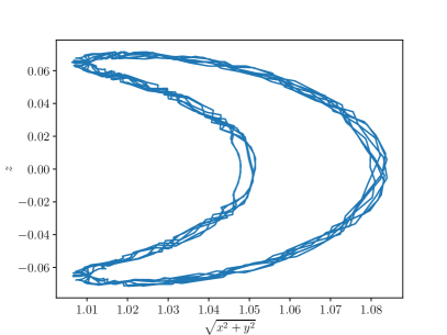
(a) GIGI2

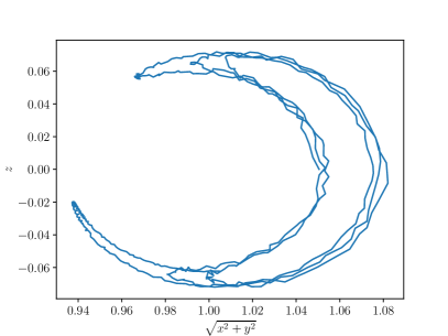
(b) RK4

Figure 1: Particle orbit in the poloidal plane of a tokamak obtained by the GIGI2 and RK4 method.

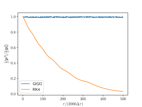
Figure 2: Evolution of $\frac{1}{2}|\mathbf{p}|^{2}$ of the charged particle in a tokamak calculated by the GIGI2 and RK4 method.

4.2 Accelerator Field

The second example is a charged particle in a model linear accelerator configuration with

$$\mathbf{A}\left(x,y,z,t\right) = \frac{B_{0}}{2a}\sin\left(k_{z}z\right)\left(x^{2}-y^{2}\right)\mathbf{e}_{z}~{},$$ (82)

$$\phi\left(x,y,z,t\right) = \phi_{0}\sin\left(k_{r}z-\omega t\right)~{}.$$ (83)

Here, $\mathbf{A}$ is the periodic quadrupole focusing field in the transverse direction, $\phi$ provides the accelerating radio frequency (RF) field in the longitudinal direction, and $a$ is the radius of the transverse direction. The normalization of physical variables used in the calculation is the same as that listed in Tab. 1. The normalized external electromagnetic fields are

$$\mathbf{B}\left(x,y,z,t\right) = \frac{\mathrm{c}}{a\Omega}\sin\left(k_{z}\mathrm{c}z/\Omega\right)\left(y\mathbf{e}_{x}-x\mathbf{e}_{y}\right)~{},$$ (84)

$$\mathbf{E}\left(x,y,z,t\right) = -\frac{\Omega\phi_{0}q}{m_{0}\mathrm{c}}k_{r}\cos\left(k_{r}\mathrm{c}z/\Omega-\omega t/\Omega\right)\mathbf{e}_{z}~{}.$$ (85)

First, the longitudinal accelerating field $\mathbf{E}$ is turned off, and particle’s dynamics in the quadrupole focusing lattice is examined. Simulation parameters are chosen as

$$\frac{\mathrm{c}}{a\Omega} = 30~{},$$

$$k_{z}\mathrm{c}z/\Omega = 7.5,$$

$$\mathbf{x}_{t=0} = [2.667\times 10^{-3},2.667\times 10^{-3},0]~{},$$

$$\left.\frac{\mathrm{d}\mathbf{x}}{\mathrm{d}t}\right|_{t=0} = [-0.001,0.001,0.9]~{},$$

$$\Delta\tau = 0.1~{}.$$

The total number of time steps is 800. Particle’s orbit and error on the Hamiltonian are plotted in Figs. 3 and 4. It is observed that particle’s orbit obtained by the GIGI2 is stable, and particle dynamics in the transverse direction is the betatron oscillation, as expected Davidson01-all ; Qin13PRL2 ; Qin14-044001 ; Qin15-056702 . The error on the Hamiltonian is globally bounded by a small number for the GIGI2. On the other hand, the RK4 method fails to generate the correct orbit, and its error on the Hamiltonian grows without bound. We note that the conservation of the Hamiltonian defined in Eq. (10) means preserving the mass-shell condition. The unbounded growth of the error on the Hamiltonian for the RK4 method implies that the numerical solution drift away from the mass-shell condition, which is physically incorrect.

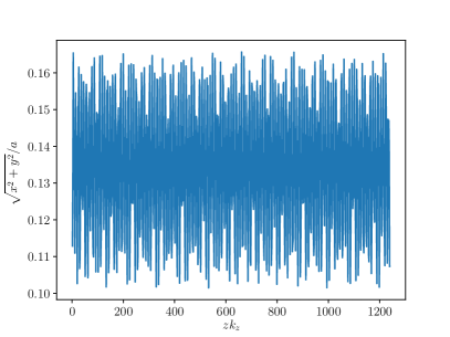
(a) GIGI2

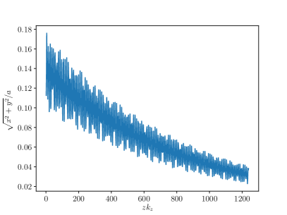
(b) RK4

Figure 3: Particle orbit in a model accelerator simulated by the GIGI2 (a) and RK4 (b) method.

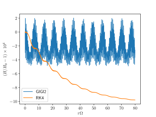
Figure 4: Evolution of the Hamiltonian $H$ of the particle in a model accelerator calculated by the GIGI2 and RK4 method.

Next, we turn on the accelerating field. The parameters are chosen as

$$\omega/\Omega = 0.1~{},$$ (86)

$$k_{r}\mathrm{c}/\Omega \approx 0.1111~{},$$ (87)

$$\frac{\Omega\phi_{0u}q}{m_{0u}\mathrm{c}}k_{r} = -0.04~{},$$ (88)

and the total number of time steps is 6400. Initially the phase speed of the electric wave is the same as the speed of the particle in the $\mathbf{e}_{z}$ direction, i.e., $\mathrm{d}z/\mathrm{d}t$. The evolution of particle orbit and Lorentz factor $\gamma$ obtained by the GIGI2 and RK4 methods are plotted in Fig. 5. It shows that the particle is accelerated at the beginning, and then decelerated and accelerated alternatively due to the phase mis-matching and matching. The RK4 method is able to calculate correctly the energy of particle, however it fails to compute the correct orbit in the transverse direction.

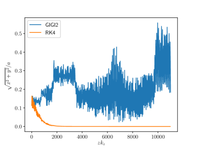
(a) Particle orbit

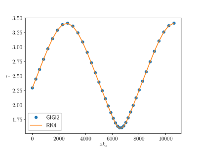
(b) Lorentz factor $\gamma$

Figure 5: Evolution of the particle orbit (a) and Lorentz factor $\gamma$ (b) calculated by the GIGI2 and RK4 method.

5 Conclusion

In this paper, we have developed a set of explicit high-order gauge-independent noncanonical symplectic integrators for relativistic charged particle dynamics. These algorithms preserve exactly a 8D noncanonical symplectic structure, and displayed long-term accuracy and fidelity. Compared with the standard implicit symplectic schemes for relativistic charged particles, the present schemes are high-order and explicit. Due to their gauge-independent property, these algorithms do not require the knowledge of vector and scalar potentials. This is more convenient for problems where only electromagnetic fields are given.

References

• (1) T. Lee, Can time be a discrete dynamical variable?, Phys. Lett. B 122 (1983) 217.
• (2) R. D. Ruth, A canonical integration technique, IEEE Trans. Nucl. Sci 30 (1983) 2669.
• (3) K. Feng, On difference schemes and sympletic geometry, in: K. Feng (Ed.), the Proceedings of 1984 Beijing Symposium on Differential Geometry and Differential Equations, Science Press, 1985, pp. 42–58.
• (4) K. Feng, Difference schemes for Hamiltonian formalism and symplectic geometry, J. Comput. Maths. 4 (1986) 279–289.
• (5) T. Lee, Difference equations and conservation laws, J. Statis. Phys. 46 (1987) 843.
• (6) A. P. Veselov, Integrable discrete-time systems and difference operators, Funkc. Anal. Priloz. 22 (1988) 1.
• (7) H. Yoshida, Construction of higher order symplectic integrators, Physics Letters A 150 (5) (1990) 262–268.
• (8) E. Forest, R. D. Ruth, 4th-order symplectic integration, Physica D 43 (1990) 105–117.
• (9) P. J. Channell, C. Scovel, Symplectic integration of Hamiltonian systems, Nonlinearity 3 (1990) 231–259.
• (10) J. Candy, W. Rozmus, A symplectic integration algorithm for separable Hamiltonian functions, Journal of Computational Physics 92 (1991) 230–256.
• (11) Y.-F. Tang, The symplecticity of multi-step methods, Computers & Mathematics with Applications 25 (1993) 83–90.
• (12) J. M. Sanz-Serna, M. P. Calvo, Numerical Hamiltonian Problems, Chapman and Hall, London, 1994.
• (13) Z. Shang, Kam theorem of symplectic algorithms for hamiltonian systems, Numerische Mathematik 83 (1999) 477–496.
• (14) J. E. Marsden, M. West, Discrete mechanics and variational integrators, Acta Numer. 10 (2001) 357–514.
• (15) E. Hairer, C. Lubich, G. Wanner, Geometric Numerical Integration: Structure-Preserving Algorithms for Ordinary Differential Equations, Springer, New York, 2002.
• (16) K. Feng, M. Qin, Symplectic Geometric Algorithms for Hamiltonian Systems, Springer-Verlag, 2010.
• (17) J. Squire, H. Qin, W. M. Tang, Geometric integration of the vlasov-maxwell system with a variational particle-in-cell scheme, Physics of Plasmas 19 (8) (2012) 084501.
• (18) J. Xiao, J. Liu, H. Qin, Z. Yu, A variational multi-symplectic particle-in-cell algorithm with smoothing functions for the vlasov-maxwell system, Phys. Plasmas 20 (10) (2013) 102517.
• (19) M. Kraus, Variational integrators in plasma physics, arXiv:1307.5665.
• (20) E. Evstatiev, B. Shadwick, Variational formulation of particle algorithms for kinetic plasma simulations, Journal of Computational Physics 245 (2013) 376–398.
• (21) B. A. Shadwick, A. B. Stamm, E. G. Evstatiev, Variational formulation of macro-particle plasma simulation algorithms, Physics of Plasmas 21 (2014) 055708.
• (22) J. Xiao, J. Liu, H. Qin, Z. Yu, N. Xiang, Variational symplectic particle-in-cell simulation of nonlinear mode conversion from extraordinary waves to bernstein waves, Physics of Plasmas 22 (9) (2015) 092305.
• (23) J. Xiao, H. Qin, J. Liu, Y. He, R. Zhang, Y. Sun, Explicit high-order non-canonical symplectic particle-in-cell algorithms for vlasov-maxwell systems, Physics of Plasmas 22 (11) (2015) 112504.
• (24) H. Qin, Y. He, R. Zhang, J. Liu, J. Xiao, Y. Wang, Comment on "hamiltonian splitting for the vlasov-maxwell equations", Journal of Computational Physics 297 (2015) 721 – 723. doi:http://dx.doi.org/10.1016/j.jcp.2015.04.056.
URL http://www.sciencedirect.com/science/article/pii/S0021999115003265
• (25) Y. He, H. Qin, Y. Sun, J. Xiao, R. Zhang, J. Liu, Hamiltonian time integrators for vlasov-maxwell equations, Physics of Plasmas 22 (12) (2015) 124503. doi:10.1063/1.4938034.
• (26) H. Qin, J. Liu, J. Xiao, R. Zhang, Y. He, Y. Wang, Y. Sun, J. W. Burby, L. Ellison, Y. Zhou, Canonical symplectic particle-in-cell method for long-term large-scale simulations of the vlasov-maxwell equations, Nuclear Fusion 56 (1) (2016) 014001.
URL http://stacks.iop.org/0029-5515/56/i=1/a=014001
• (27) S. D. Webb, A spectral canonical electrostatic algorithm, Plasma Physics and Controlled Fusion 58 (2016) 034007.
• (28) M. Kraus, K. Kormann, P. J. Morrison, E. Sonnendrücker, Gempic: Geometric electromagnetic particle-in-cell methods, Journal of Plasma Physics 83 (4).
• (29) X. Jianyuan, Q. Hong, L. Jian, Structure-preserving geometric particle-in-cell methods for vlasov-maxwell systems, Plasma Science and Technology 20 (11) (2018) 110501.
• (30) J. Xiao, H. Qin, P. J. Morrison, J. Liu, Z. Yu, R. Zhang, Y. He, Explicit high-order noncanonical symplectic algorithms for ideal two-fluid systems, Physics of Plasmas 23 (11) (2016) 112107.
• (31) E. S. Gawlik, P. Mullen, D. Pavlov, J. E. Marsden, M. Desbrun, Geometric, variational discretization of continuum theories, Physica D: Nonlinear Phenomena 240 (21) (2011) 1724–1760.
• (32) D. Pavlov, P. Mullen, Y. Tong, E. Kanso, J. E. Marsden, M. Desbrun, Structure-preserving discretization of incompressible fluids, Physica D: Nonlinear Phenomena 240 (6) (2011) 443–458.
• (33) Y. Zhou, H. Qin, J. Burby, A. Bhattacharjee, Variational integration for ideal magnetohydrodynamics with built-in advection equations, Physics of Plasmas 21 (10) (2014) 102109.
• (34) Y. Zhou, Y.-M. Huang, H. Qin, A. Bhattacharjee, Formation of current singularity in a topologically constrained plasma, Phys. Rev. E 93 (2016) 023205. doi:10.1103/PhysRevE.93.023205.
URL http://link.aps.org/doi/10.1103/PhysRevE.93.023205
• (35) H. Qin, X. Guan, Variational symplectic integrator for long-time simulations of the guiding-center motion of charged particles in general magnetic fields, Physical Review Letters 100 (3) (2008) 035006.
• (36) H. Qin, X. Guan, W. M. Tang, Variational symplectic algorithm for guiding center dynamics and its application in tokamak geometry, Physics of Plasmas 16 (4) (2009) 042510.
• (37) X. Guan, H. Qin, N. J. Fisch, Phase-space dynamics of runaway electrons in tokamaks, Physics of Plasmas 17 (9) (2010) 092502.
• (38) J. Li, H. Qin, Z. Pu, L. Xie, S. Fu, Variational symplectic algorithm for guiding center dynamics in the inner magnetosphere, Physics of Plasmas 18 (5) (2011) 052902.
• (39) R. Zhang, J. Liu, Y. Tang, H. Qin, J. Xiao, B. Zhu, Canonicalization and symplectic simulation of the gyrocenter dynamics in time-independent magnetic fields, Physics of Plasmas 21 (3) (2014) 032504.
• (40) J. Squire, H. Qin, W. M. Tang, Gauge properties of the guiding center variational symplectic integrator, Physics of Plasmas 19 (5) (2012) 052501.
• (41) J. Burby, C. Ellison, Toroidal regularization of the guiding center lagrangian, Physics of Plasmas 24 (11) (2017) 110703.
• (42) C. L. Ellison, J. M. Finn, J. W. Burby, M. Kraus, H. Qin, W. M. Tang, Degenerate variational integrators for magnetic field line flow and guiding center trajectories, Physics of Plasmas 25 (5) (2018) 052502.
• (43) Y. He, Y. Sun, Z. Zhou, J. Liu, H. Qin, Explicit non-canonical symplectic algorithms for charged particle dynamics, arXiv:1509.07794.
• (44) Y. He, Z. Zhou, Y. Sun, J. Liu, H. Qin, Explicit k-symplectic algorithms for charged particle dynamics, Physics Letters A 381 (6) (2017) 568–573.
• (45) Z. Zhou, Y. He, Y. Sun, J. Liu, H. Qin, Explicit symplectic methods for solving charged particle trajectories, Physics of Plasmas 24 (5) (2017) 052507.
• (46) R. Zhang, H. Qin, Y. Tang, J. Liu, Y. He, J. Xiao, Explicit symplectic algorithms based on generating functions for charged particle dynamics, Physical Review E 94 (1) (2016) 013205.
• (47) R. Zhang, Y. Wang, Y. He, J. Xiao, J. Liu, H. Qin, Y. Tang, Explicit symplectic algorithms based on generating functions for relativistic charged particle dynamics in time-dependent electromagnetic field, Physics of Plasmas 25 (2) (2018) 022117.
• (48) J. P. Boris, R. A. Shanny, Proceedings: Fourth Conference on Numerical Simulation of Plasmas, November 2, 3, 1970, Naval Research Laboratory, 1972.
• (49) H. Qin, S. Zhang, J. Xiao, J. Liu, Y. Sun, W. M. Tang, Why is boris algorithm so good?, Physics of Plasmas 20 (8) (2013) 084503.
• (50) C. Ellison, J. Burby, H. Qin, Comment on "symplectic integration of magnetic systems": A proof that the boris algorithm is not variational, Journal of Computational Physics 301 (2015) 489 – 493. doi:http://dx.doi.org/10.1016/j.jcp.2015.09.007.
URL http://www.sciencedirect.com/science/article/pii/S0021999115005884
• (51) R. Zhang, J. Liu, H. Qin, Y. Wang, Y. He, Y. Sun, Volume-preserving algorithm for secular relativistic dynamics of charged particles, Physics of Plasmas 22 (4) (2015) 044501.
• (52) Y. He, Y. Sun, J. Liu, H. Qin, Volume-preserving algorithms for charged particle dynamics, Journal of Computational Physics 281 (2015) 135–147.
• (53) Y. He, Y. Sun, R. Zhang, Y. Wang, J. Liu, H. Qin, High order volume-preserving algorithms for relativistic charged particles in general electromagnetic fields, Physics of Plasmas 23 (9) (2016) 092109.
• (54) Y. He, Y. Sun, J. Liu, H. Qin, Higher order volume-preserving schemes for charged particle dynamics, Journal of Computational Physics 305 (2016) 172.
• (55) X. Tu, B. Zhu, Y. Tang, H. Qin, J. Liu, R. Zhang, A family of new explicit, revertible, volume-preserving numerical schemes for the system of lorentz force, Physics of Plasmas 23 (2016) 122514. doi:10.1063/1.4972878.
• (56) A. V. Higuera, J. R. Cary, Structure-preserving second-order integration of relativistic charged particle trajectories in electromagnetic fields, Physics of Plasmas 24 (5) (2017) 052104. doi:10.1063/1.4979989.
URL http://adsabs.harvard.edu/abs/2017PhPl...24e2104H
• (57) H. Goldstein, Classical mechanics, Pearson Education India, 2011.
• (58) J. E. Marsden, T. Ratiu, Introduction to mechanics and symmetry: a basic exposition of classical mechanical systems, Vol. 17, Springer Science & Business Media, 2013.
• (59) Y. He, Y. Sun, H. Qin, J. Liu, Hamiltonian particle-in-cell methods for vlasov-maxwell equations, Physics of Plasmas 23 (9) (2016) 092108.
• (60) J. E. Marsden, G. W. Patrick, S. Shkoller, Multisymplectic geometry, variational integrators, and nonlinear pdes, Communications in Mathematical Physics 199 (2) (1998) 351–395.
• (61) R. C. Davidson, H. Qin, Physics of Intense Charged Particle Beams in High Energy Accelerators, Imperial College Press and World Scientific, 2001.
• (62) H. Qin, R. C. Davidson, M. Chung, J. W. Burby, Phy. Rev. Lett. 111 (2013) 104801.
• (63) H. Qin, R. C. Davidson, J. W. Burby, M. Chung, Analytical methods for describing charged particle dynamics in general focusing lattices using generalized courant-snyder theory, Phys. Rev. ST Accel. Beams 17 (2014) 044001. doi:10.1103/PhysRevSTAB.17.044001.
• (64) H. Qin, M. Chung, R. C. Davidson, J. W. Burby, Spectral and structural stability properties of charged particle dynamics in coupled lattices, Physics of Plasmas 22.