Whisper: Fast Flooding for Low-Power Wireless Networks

Abstract.

This paper presents Whisper, a fast and reliable protocol to flood small amounts of data into a multi-hop network. Whisper makes use of synchronous transmissions, a technique first introduced by the Glossy flooding protocol. In contrast to Glossy, Whisper does not let the radio switch from receive to transmit mode between messages. Instead, it makes nodes continuously transmit identical copies of the message and eliminates the gaps between subsequent transmissions. To this end, Whisper embeds the message to be flooded into a signaling packet that is composed of multiple packlets – where a packlet is a portion of the message payload that mimics the structure of an actual packet. A node must intercept only one of the packlets to detect that there is an ongoing transmission and that it should start forwarding the message. This allows Whisper to speed up the propagation of the flood, and thus, to reduce the overall radio-on time of the nodes. Our evaluation on the FlockLab testbed shows that Whisper achieves comparable reliability but 2x lower radio-on time than Glossy. We further show that by embedding Whisper in an existing data collection application, we can more than double the lifetime of the network.

1. Introduction

Many application scenarios for low-power wireless networks require the reliable and fast exchange of small data values. Examples include the dissemination of parameters – e.g., the set-point of a valve – in industrial control systems or smart buildings. In these settings, the communication is either periodic or event-driven. Approaches like Glossy (16) or LWB (15) can be used to reliably and quickly share data periodically in a low-power wireless network. Crystal (18; 19) and other approaches (36; 19; 24; 14; 41; 26; 29) extend Glossy to event-driven systems by periodically sampling the network for potential events.

In this paper, we present Whisper, a novel communication primitive that addresses the challenge of quickly and efficiently sharing small amounts of information in either periodic or event-based application scenarios. Whisper relies on synchronous transmissions to provide fast and energy-efficient communication in low-power wireless multi-hop networks. First, Whisper integrates the flood – consisting of multiple replicated packets as in Glossy – into a single packet transmission. This reduces the duration of a flood, eliminates gaps, i.e, the radio turnaround time, and thereby allows Whisper to reduce radio-on time and energy consumption. Second, its compact flooding format and the lack of gaps between packets enable Whisper to introduce energy-efficient sampling strategies, i.e, the ability to sample the channel for a packet and not, as done in Glossy, LWB, Crystal and most others protocols to rely on idle listening of the radio.

Whisper can be used as “standalone” dissemination protocol for small data and as service for other protocols, e.g., as an efficient wake-up primitive to reduce the protocol’s idle listening overhead. The latter is the case in the event-based transmission of large data packets. In such scenarios, the nodes listen to potential packets for a predefined interval before turning the radio off. Using Glossy-like protocols, the length of this interval depends on the packet size, the number of hops in the network, and the number of packet repetitions $N_{tx}$. For example, it would take Glossy almost 67 ms to disseminate a 127 byte packet in a 6-hop network with $N_{tx}=3$. Thus, all nodes must keep the radio turned on for this amount of time, even when no packet is disseminated. Using Whisper, the nodes keep their radio on for at most a Whisper slot, which is less than 3 ms in a 6-hop network. Only if they have received a packet during the Whisper slot, they await the actual data packet afterward. Otherwise, they keep their radio turned off. Thus, using Whisper, nodes only communicate when they have an event to share.

In summary, Whisper is designed around three cornerstones:

• Whisper compacts the network flood into a single packet without “gaps” to reduce latency and radio-on time and to enable efficient sampling.

• Whisper employs strategies for sampling so that nodes can energy-efficiently determine whether there is data to exchange during a round or not.

• Whisper exploits synchronous transmissions for fast and reliable flooding.

We show the efficiency of Whisper as primitive for fast and reliable network-wide flooding of small amounts of data by evaluating it on the publicly available FlockLab testbed. For example, in Whisper nodes can determine whether a flood is ongoing within less than 3 milliseconds in a 6-hop network, whereas in Crystal and in several solutions of the EWSN dependability competitions, nodes are awake for the duration of the network flood, which on FlockLab, for example, commonly takes 5 milliseconds. We further show that Whisper has an up to 50% higher network lifetime than Glossy and it can increase the network lifetime of Crystal by a factor of 2.3 when used as wake-up service within Crystal.

The remainder of this paper is structured as follows. We present a high-level overview of Whisper in Sec. 2 and discuss relevant details of its design in Sec. 3. Using our implementation for TelosB nodes in Contiki, we compare Whisper in various dissemination scenarios with Glossy in Sec. 4 and use Whisper as wake-up primitive in Crystal in Sec. 5. A discussion of related work follows in Sec. 6 and Sec. 7 concludes the paper.

2. Whisper: How it works

Figure 1. Format of a signaling packet. The gray-shadowed footer at the end of the packet is created only when the radio is used in buffered mode.

At its core, Whisper is a communication primitive that allows to quickly and reliably flood data into a multi-hop network. In the following, we describe the three building blocks of Whisper’s design: packlets, direction-aware channel sampling, and synchronous transmissions.

Signaling packet and packlets

In Whisper, a node that needs to send data – hereafter referred to as the sender – transmits a signaling packet, which looks as depicted in Fig. 1. It consists of several packlets, whereas a packlet is a piece of message payload that has the structure of an actual IEEE 802.15.4 packet, including preamble, start-of-frame delimiter (SFD) and footer. Whisper’s signaling packet, thus, mimics a train of short, identical packets being sent continuously by the radio, as illustrated in Fig. 2a.

This is a core difference between Whisper and, e.g., Glossy (16). In Glossy– and in all protocols that build upon it – the nodes continuously switch between sending and receiving mode, and thus, leave “gaps” between two transmissions, as depicted in Fig. 2c. The absence of such gaps significantly increases the speed at which the network flood can propagate and, thus, it reduces the time nodes must keep their radio on.

It is also worth noting that there exist other techniques, e.g., (24; 14; 26), that modified Glossy to make it transmit packets consecutively instead of alternating between reception and transmission. These existing approaches, however, still suffer from the existence of the gaps because the radio transceiver must perform the RX/TX turnaround each time after packet transmission completes. By embedding packlets in the payload of a single signaling packet, Whisper completely eliminates gaps between consecutive transmissions, because there is no RX/TX turnaround.

While Whisper can support payloads of arbitrary length, it is best suited to flood small amounts of data, as we also discuss in Sec. 3.9. Small payloads occur frequently in real scenarios, e.g., when a configuration parameter, which may be coded using just a few bits, must be communicated to all nodes in a network. More importantly, Whisper can be used as a very efficient signaling primitive to, e.g., notify to all nodes in a network that they must stay awake to help forwarding incoming data packets. In this scenario, no data or only very little data is actually transmitted and thus a small payload size does not represent a limiting factor.

(a) Whisper.

(b) Whisper with lazy sampling.

(c) Glossy.

Figure 2. Whisper eliminates gaps. The time needed to switch the radio between receive (RX) and transmit (TX) mode (and vice versa) causes communication “gaps” to occur in Glossy. By transmitting a log train of packlets, Whisper does not need to perform the RX/TX turnaround and thus eliminates these gaps.

Figure 3. Whisper’s operation. Nodes receive a packlet, process it while turning their radio to transmit mode and afterwards transmit their signaling packet.

Sampling strategy

For nodes to be able to detect the presence of a signaling packet, they must regularly switch their radios on and check the channel for incoming transmissions. The more often this channel check is performed – and the longer each check lasts – the higher is the duty cycle of the nodes and thus their energy consumption. The possibility to design thrifty sampling strategies – which is opened up by the use of packlets – is thus instrumental to reduce the overall radio-on time and thus the duty cycle of nodes running Whisper.

A straightforward sampling strategy – to which we refer to as lazy sampling (see Fig. 2b) – consists in making all nodes switch their radios on at the beginning of a communication slot. This strategy is used in Glossy and other approaches such as LWB (15) or Crystal (18) and can be used in Whisper too. When adopting lazy sampling, nodes must wait for an incoming transmission long enough so that a message from the initiator can propagate through the entire network. This can, however, take several milliseconds in a network of few hops and represents a high cost in terms of energy consumption, especially if no packet is transmitted.

To cope with this problem, Whisper uses an alternative sampling strategy – which we dub direction-aware sampling. It exploits the fact that in many practical scenarios the network topology is usually fixed or changes slowly and that data traffic flows in one direction only – e.g., from an initiator to all other nodes in a network in a data dissemination scenario or from a random node in the network to a central sink node in case of event-driven aperiodic communication. Thus, nodes can estimate their distance in hops from the sender or destination, respectively, and switch on their radios only when a signaling packet is likely to “pass-by”, as shown in Fig. 2a.

Synchronous transmissions

To ensure a fast and reliable propagation of the signaling packet, Whisper exploits synchronous transmissions. When a neighbor of the sender turns its radio on, it needs to intercept only one of the packlets to detect the existence of a signaling packet. If no packlet is detected, the node switches its radio off to save energy. If a packlet is instead successfully received, the node keeps its radio on and helps propagating the signaling packet. It does so by joining the ongoing synchronous transmission with its own signaling packet, which is again a single packet made of multiple packlets. To this end, a node that starts sending a signaling packet must ensure that its own packlets overlap with the packlets that are already being transmitted by other nodes.

Whisper takes special account of scenarios in which nodes share the same data, e.g., when a controller disseminates a new configuration parameter or when Whisper is used as wake-up primitive. In these cases, packlets sent by nearby nodes must fulfill two conditions: they must be identical and must be sent at almost exactly the same time instant, as schematically illustrated in Fig. 2a. We discuss in Sec. 3 how Whisper manages to fulfill both these conditions.

Whisper also supports the concurrent transmission of different data. The procedures for sending identical data packets and different data packets are identical. The latter case, however, relies on the capture effect instead of constructive interference.

3. Whisper: A Closer Look

After having presented the core design elements of Whisper in the previous section, we now discuss in detail its most relevant features.

3.1. The signaling packet

The design of the signaling packet as shown in Fig. 1 makes Whisper able to send a train of packets back-to-back, i.e., without any gaps between consecutive transmissions. We argue that this is an essential stepping stone to: (a) lower the duration of a network flood; (b) enable sampling strategies that reduce nodes’ duty cycle; and (c) simplify the timing of synchronous transmissions.

Whisper uses the payload of the signaling packet to simulate several packets being sent back-to-back. This is achieved by the use of packlets, a technique inspired by the multi-header approach presented in (22). As illustrated in Fig. 1, a packlet in Whisper consists of at least five fields: a preamble, a 1-byte SFD, 1-byte length field, a 1-byte payload, and a 2-byte footer, which includes a Frame Check Sequence (FCS). Nonetheless, the packlet format in Whisper is user-configurable and can be changed or extended to contain, e.g., larger payloads. When a receiver starts listening for incoming packets it only needs to intercept a single preamble and SFD of one of the packlets to detect an ongoing transmission.

While the IEEE 802.15.4-compliant length of the preamble is 4 bytes, in some radios – e.g., the CC2420 (40) – both the preamble length and the SFD are configurable parameters. To reduce the total length of a signaling packet, and thus, decrease the radio-on time of the nodes, Whisper’s default implementation sets the length of the preamble to 2 bytes. While this assumes that Whisper can exploit low-level features of the transceiver and makes it non-IEEE 802.15.4-compliant, we believe that it is important to explore the potential of Whisper’s design beyond current technological limits. Several other authors have indeed explored before us non-IEEE 802.1.5.4-compliant techniques to design energy-efficient protocols (31; 13; 8). Nonetheless, Whisper can operate with a preamble of arbitrary length and can thus, if required, also be used with a standard-compliant preamble of 4 bytes. While a longer preamble affects performance, we show in Sec. 4 that Whisper outperforms Glossy also with a preamble length of 4 bytes.

Given the above description, a packlet is by default 7 bytes long. Since IEEE 802.15.4 radios transmit at a rate of 250 kbit/s, the transmission of one packlet– henceforth denoted with $T_{packlet}$ – lasts 224 $\mu$s. The sender sends $N_{tx}$ packlets and its total transmission time with $N_{tx}=3$ is thus 672 $\mu$s. The radio of other nodes in the network is instead active for at least the duration of $N_{tx}+2$ packlets. This is because, as depicted in Fig. 2a, before being able to send its $N_{tx}$ packlets a node must first receive one packlet and then switch the radio from receive to transmit mode, thereby adding the duration of 2 packlets to the total time needed to transmit $N_{tx}$ packlets. Further, nodes must sample the channel, which further adds to the time they must keep the radio on. With direction-aware sampling, for instance, nodes persist in idle listening for the duration of roughly one packlet, thus, bringing the otal radio-on time to $(N_{tx}+2+1)\cdot T_{packlet}$, i.e., 1,344 ms by setting $T_{packlet}=$ 224 $\mu$s.

In contrast, nodes running Glossy in the same scenario must keep their radio on for at least $2N_{tx}$ transmissions. This is because, as shown in Fig. 2c, a node in Glossy both receives and transmits a packet $N_{tx}$ times. Assuming that also Glossy sends packets with a 1-byte payload – and that a Glossy packet is as long as a packlet– each node actively transmits or receives for $2N_{tx}T_{packlet}$, i.e., 1.344 ms when $N_{tx}=3$. Glossy must, however, also continuously switch between receive and transmit mode, as illustrated in Fig. 2c. This RX/TX turnaround of the radio takes 192 $\mu$s (17) and nodes must turn the radio from receive to transmit mode $N_{tx}-1$ times, which adds almost 1 ms (i.e., 960 $\mu$s) of additional radio on time. The radio-on time of Glossy is thus almost twice as long as that of Whisper (2,304 ms vs. 1,344 ms) – even though we did not account for the time spent in idle listening by nodes running Glossy nor for Glossy’s software delay, which should be added to the RX/TX turnaround time. We also did not consider – neither in the calculation above nor in Fig. 2 – the guard times that are present in both Whisper and Glossy. A guard interval is usually short and appears only once at the beginning of the idle listening phase. It, thus, has only little influence on the computation presented above.

This back-of-the-envelope calculation shows that the superior performance of Whisper with respect to Glossy– discussed in detail in Sec. 4.2 – is mainly due to the fact that Whisper eliminates the gaps between consecutive transmissions. This advantage persists even if Whisper is used with lazy sampling, as in this case the time spent in idle listening is roughly the same as for Glossy.

In the example discussed above, we assume Glossy packets with a payload of 1 byte. The payload of standard Glossy packets is, however, 4 bytes: a 2 byte sequence number, a 1 byte Glossy header, and a 1 byte relay counter (16). We reduce the payload size to 1 byte (we keep only the field relay_counter), to avoid penalizing Glossy due to its larger payload size. This also allows us to show – in Sec. 4 – that shortening the payload size in Glossy is not sufficient to make it more efficient than Whisper.

3.2. Sending identical packlets

Whisper natively takes special account for scenarios in which nodes share identical data. For these cases, sending identical packets is a necessary condition for constructive interference to occur (or more precisely for packets not to interfere destructively) when synchronous transmissions are used. In Whisper, this translates in ensuring that all packlets sent at the same time are identical.

The only value that changes across different packlets in the same signaling packet is the counter $c$, which is the 1-byte payload of each packlet. As illustrated in Fig. 1, the $1$st packlet has counter $c=0$, the second $c=1$, and so on. When nodes start sending their own signaling packet, they must properly set the value of the counter $c$ of the packlets. In particular – as also shown in Fig. 3 – Whisper makes a node that receives a packlet with counter $c=i$ set the counter of its first packlet to $c=i+2$. This is because while the $c=i+1$th packlet is being transmitted, the node performs the RX/TX turnaround of the radio. In this time frame the node “misses” a packlet and must wait until the next one starts being sent before sending its own signaling packet.

Besides ensuring the values of the counter $c$ is identical for all synchronously transmitted packlets, Whisper must also properly set the length field of the packlets. This field specifies the length in bytes of the payload and the footer. For packlets that have a 1-byte payload, the length field must, thus, be set to three. This can be easily done for all packlets but the first. As highlighted in gray in Fig. 1, the packlet with counter $c=0$ “borrows” the preamble, SFD, and length field of the signaling packet. The first byte of the signaling packet, however, specifies how many bytes the radio must send before automatically ceasing to transmit. If Whisper would use this mode of operation (called buffered mode in the CC2420 (40)), the (first) length field in the signaling packet would indicate the total length of the signaling packet in bytes – which is different than three. This would cause the length field of each signaling packet to collide with the length field of synchronously sent packlets. As a consequence, destructive interference would occur and result in packet drops.

To avoid this problem, we exploit an alternative transmit mode available on certain IEEE 802.15.4 radio transceivers (including the CC2420 (40)): the TXFIFO looping mode. When set in this mode the radio ignores the length field and just continuously reads data from the radio buffer and transmits it. Once the content of the buffer has been sent, the radio wraps around and starts to read and send the data from the beginning. This continues indefinitely until a timeout explicitly stops the transmission. Since the value of the length field is ignored when the radio operates in TXFIFO looping mode, Whisper can set the first length field to the length of a packlet – instead that to the length of the signaling packet– thus completely overcoming the problem described above.

While this mode of operation may not be available on all IEEE 802.15.4 transceivers, which limits the portability of Whisper, we believe that it is important to explore novel design ideas notwithstanding current technological limits and protocol standards. We further plan to explore an alternative approach to avoid the TXFIFO looping mode: using byte-wise transmission power control to send the length field using the smallest possible transmit power (32). When evaluating the performance of Whisper in Sec. 4, we, nonetheless, explicitly consider a fully IEEE 802.15.4-compliant version of the protocol, called Whisper (compliant), which we describe in Sec. 3.6.

Further, Whisper is not limited for sharing identical data. Related work has already shown the efficiency of synchronously transmitting different data (21; 18; 6; 43) by relying on the capture effect. Letting the nodes flood different data with Whisper, indeed, also relaxes the need for support of the TXFIFO looping mode. The advantage of Whisper compared to existing solutions is, still, the absence of gaps resulting in a short flooding duration and thus, efficient sampling.

3.3. Sending packlets synchronously

In the previous subsection we mentioned that after receiving a packlet (with counter value $c_{i}$), a node must wait for an entire $T_{packlet}$ before sending its first packlet (with counter $c_{i}+2$). This is because while packlet $c_{i}+1$ is on the air, the node must perform the RX/TX turnaround of the radio, which lasts $T_{turn}=192$ $\mu$s for IEEE 802.15.4 radios (17). This leaves a wait time $T_{wait}=T_{packlet}-T_{turn}-T_{d}$, whereas $T_{d}$ is the time that elapses between the rising SFD edge of a sender during transmission and the corresponding rising SFD edge of a receiver during reception.

The existence of $T_{d}$ is due to the fact that the reception of a pack(l)et lasts slightly longer than its transmission. This data delay is a common phenomenon in wireless radios, and each transceiver has a specific latency of the RX and TX paths, which is reported in the data sheets. If not compensated for, the existence of $T_{d}$ would make nodes start sending the next packlet before receivers have completed the reception of the previous one. Including propagation delay, $T_{d}$ is reported to be $3<T_{d}\leqslant 3.6$ $\mu$s (40; 42; 20) and is, thus, non-negligible. In Whisper, we set $T_{d}=3$ $\mu$s.

The existence of this fixed wait time is a further difference between Whisper and Glossy. Indeed, Glossy aims at re-sending a packet as quickly as possible after receiving it (i.e., immediately after the RX/TX turnaround). This is because the longer nodes wait to retransmit a packet, the stronger MCU clock instabilities become relevant and can, thus, cause transmissions of different nodes to misalign (16). This so-called software delay in Glossy is $23$ $\mu$s. In Whisper, if we assume a payload of 1 byte and a preamble of 2 bytes, then $T_{packlet}=224$ $\mu$s and, thus, $T_{wait}=29$ $\mu$s. Although the values of $T_{wait}$ and of Glossy’s software delay are relatively close to each other, the latter does not depend on the length of the packet whereas it does in the case of Whisper. The wait time is, thus, more critical for Whisper than for Glossy.

To cope with this issue we employ Flock, a recently presented clock compensation approach for low-power nodes (7). Flock compensates for instabilities in the digitally controlled oscillator (DCO) that drives the MCU of many low-power hardware platforms. It, thus, makes Whisper able to ensure that packlet transmissions align within the 0.5 $\mu$s window notwithstanding the existence of $T_{wait}$ and even if $T_{wait}$ is significantly longer than 29 $\mu$s. This, in turn, makes Whisper robust even with long packlets and in challenging environments with highly unstable DCO clocks, like those considered in (5).

3.4. Lazy sampling

A straightforward way to maximize the probability that a node intercepts a signaling packet, even in scenarios with high node mobility, consists in making the node keep its radio in idle listening for the entire duration of a Whisper slot. This is the time interval during which a Whisper flood is executed and during which – like in Glossy and other protocols based on synchronous transmissions – all other application tasks executing the hosting platform are suspended.

The length of the slot – indicated as $T_{slot}$ – is a protocol parameter and should be set depending on the expected network diameter. In particular, it holds:

(1) $$T_{slot}=(2d_{net}+N_{tx})\cdot T_{packlet},$$

where $d_{net}$ is the network diameter and $T_{packlet}$ is the time needed to send a packlet. The first addend in Eq. 1 accounts for the fact that Whisper progress at a “speed” of 2 packlets per hop, as illustrated in Fig. 2a. The second addend instead considers that at the last hop, after the first packlet has been transmitted a node must still transmit $N_{tx}-1$ packlets. If Whisper is used in a network of 6 hops and with $N_{tx}=3$ and $T_{packlet}$ = 224 $\mu$s (1 byte payload), a slot length of 4,48 ms would be sufficient. In practical settings, however, it is recommendable to use a slightly larger value to account for synchronization drifts and other issues. In the experiments presented in Sec. 4, for instance, we use $T_{slot}=5$ ms.

Irrespectively of the type of sampling used, once a Whisper slot ends nodes schedule their next wake-up according to the needs of the application. If, for instance, it must be checked every $5$ minutes if there is an update by the initiator, nodes will reschedule their wake-up accordingly at a time instant $t^{*}_{start}$ that is 5 minutes away from the beginning of the slot. To account for possible synchronization errors, Whisper uses as in Glossy a guard time – indicated as $T_{guard}$ – and makes the node actually switch their radio on at $t^{*}_{start}-T_{guard}$.

3.5. Direction-aware sampling

A significant drawback of the lazy sampling strategy sketched above is that it causes all nodes in the network to stay in idle listening for an entire Whisper slot – even when no signaling packet is sent. To reduce this idle listening time and thus the overall radio-on time, Whisper exploits a different strategy, which we call direction-aware sampling.

The main idea behind this strategy is to let the nodes switch their radio on only shortly before the flood is expected to “pass by”. In low-power networks, traffic often flows in one direction only, e.g., from an initiator towards all other nodes in the network in data dissemination scenarios (16; 9; 10) or from all nodes to a sink in data collection (18). If the direction of the traffic is known – hence the name direction-aware sampling – Whisper can exploit this information to run an efficient sampling strategy.

In the scenario considered in Glossy, for instance, traffic always flows from a fixed initiator to all other nodes. If Whisper is used in this scenario, the counter $c$ of the packlet received by a forwarding node depends on the distance in hops between the node and the initiator. If the topology of the network can be assumed to be static or vary slowly, this distance – and thus, the counter $c$ – can also be assumed to be constant or to vary only a little across consecutive floods. Whisper exploits this situation and lets each node keep in memory two values – $c_{min}$ and $c_{max}$ – which are estimates of the counters of the packlets with the lowest and highest counter, and thus, the “earliest” and “latest” packlet a node is expected to receive. Both values $c_{min}$ and $c_{max}$ are used by the nodes to compute when to turn the radio on and off, respectively. The value of $c_{min}$ is set to the lowest value of $c$ ever received. The value for $c_{max}$ can be computed as follows:

(2) $$c_{max}=(c_{max}+c)/2\quad\text{if: }c\geq c_{max}-2$$

The term $c_{max}-2$ in the condition of Eq. 2 accounts for the progression speed of $2$ in Whisper. Thus, Eq. 2 allows the filtering of outliers that could result in a high sampling duration, and thus, high energy consumption, while also being able to react to changing channel conditions. Underestimating $c_{max}$ would, thus, cause a node to switch off its radio too early, which in the worst case could stop the propagation of the flood. The strategy chosen to set both $c_{min}$ and $c_{max}$ are very conservative and can definitely be improved in future work. The design of Whisper actually opens up opportunities for designing further smart sampling strategies beyond the two – lazy and direction-aware – discussed in this paper.

Once $c_{min}$ and $c_{max}$ are known, a node can compute the start and the duration of its sampling interval as follows:

(3) $$t_{start}=t^{*}_{start}-T_{guard}+max(0,c_{min}-1)\cdot T_{packlet}$$

(4) $$T_{sampling}=(\lfloor c_{max}\rfloor+(N_{tx}+1))\cdot T_{packlet}-t_{start}$$

In Eq. 3, $t^{*}_{start}$ indicates the time at which the sender is expected to start its transmission, whereas $T_{guard}$ is the guard time that protects against possible synchronization drifts. When a node did not yet receive its very first packlet, it sets $c_{min}=0$ and $T_{sampling}=T_{slot}$. When the first packlet with counter $c$ is received, the node sets $c_{min}=c_{max}=c$. Afterwards, the mechanisms mentioned above are used to update $c_{min}$ and $c_{max}$.

The discussion above assumes that Whisper is used in a data dissemination scenario. In Sec. 5, we show how direction-aware sampling can be applied also in a data collection scenario.

3.6. Whisper (compliant)

The standard version of Whisper described above exploits low-level mechanisms of the radio transceiver. For the sake of completeness, we consider in our evaluation also an IEEE-802.15.4-compliant version of Whisper, called Whisper (compliant). This version uses a 4-byte preamble and the radio in buffered mode, which has the following two consequences. First, the first length field of the signaling packet must be set to the actual length of the payload and will, thus, collide with the length field of synchronously sent packlets. This causes the first packlet of each signaling packet to be dropped, and thus, slows down the progression of the flood. In particular, Whisper (compliant) needs three instead of two packlets per hop to progress. Second, the radio hardware will set the footer of the signaling packet, i.e., the gray-shadowed footer in Fig. 1. To avoid this footer to collide with the footer of synchronously sent packlets, Whisper (compliant) makes that all nodes stop sending at the same time, so that the footers of all signaling packets align.

3.7. Resilience against external interferences

As other approaches based on synchronous transmissions, Whisper is sensitive to external interference. Common devices such as microwave ovens or Wi-Fi access points can disturb communication and significantly reduce the reliability of the protocol. Several approaches already presented in the literature show that introducing frequency diversity – in particular channel hopping – is an effective countermeasure against external interference (19; 24; 34). These techniques, especially sending each flood on a different frequency (19), are straightforward to integrate in Whisper.

3.8. Porting Whisper to other radios

Whisper exploits low-level mechanisms that are, admittedly, not available for all radio transceivers. However, the design of Whisper is still not limited to the CC2420 radio chip and the TelosB platform. The CC2520 (37) that is used in the WiSMote (2) nodes also provides the TXFIFO looping mode. Often, radio chips provide the TXFIFO looping mode functionality using a different name. For example, the Atmel AT86RF215 (4) that is deployed in the OpenMote-B calls it frame based continuous transmission or continuous transmission in the AT86RF231 chip (3) that the M3 Open Nodes and A8 Open Nodes are equipped with. The Semtech SX1211 (33) chip calls this functionality buffered mode and the default mode is here called packet mode (not to be confused with the default ’buffered mode’ of the CC2420). The CC1101 (39) that is deployed in the MSP430-CCRF (30) nodes provides three packet length modes that can be reprogrammed during receive and transmit: fixed mode, variable mode, and infinite mode. Using these modes, the CC1101 supports packet lengths that are longer than 127 bytes. Whisper can use them to avoid the transmission of the length field of the signaling packet.

For radios that do not support the TXFIFO looping mode or similar options, a software-based solution like the byte-wise transmission power control approach from Saha and Chan (32) – where the length field is transmitted with the smallest possible transmit power – as mentioned in Sec. 3.2, could be an interesting alternative approach that we plan to investigate in a future project.

3.9. Using Whisper with large payloads

(a) First hop.

(b) Third hop.

(c) Sixth hop.

Figure 4. The theoretical radio-on time for different payloads at different hops. The nodes in the first hop using Whisper and Whisper (lazy) achieve a lower radio-on time compared to the nodes running Glossy for all payload sizes. The nodes using Whisper (lazy) in the third hop exceed the radio-on time of the nodes using Glossy at 40 bytes of payload and the nodes in the sixth hop running Whisper (lazy) exceed the nodes running Glossy’s radio-on time at 15 bytes payload. Whisper achieves for all three network diameters and all payload sizes a lower radio-on time compared to Glossy.

This paper describes Whisper as quick yet energy-efficient flooding primitive for small amounts of data. However, Whisper also supports the propagation of large data, i.e., packlet lengths of 127 bytes. Using the TXFIFO looping mode, the radio returns to the beginning of the TXFIFO buffer when the radio has reached the end of the buffer. The MCU has, thus, to continuously fill the buffer while the radio continuously reads the buffer. This allows a sender to transmit packlets and signaling packets of infinite length. However, the receivers operate in buffered mode in which the length of a packlet is limited to 127 bytes (while the length of a signaling packet is still unlimited).

Even though Whisper also works for large data, the sampling strategies presented in this paper are designed for small data. For example, in the direction-aware sampling strategy, the nodes wake-up one packlet before the actually expected packlet. Transmitting and receiving a 127 byte packlet takes about 4 ms. Thus, the nodes stay in idle listening for the entire 4 ms, which is power inefficient. In applications with large data, a new sampling strategy should be designed, e.g., by letting the nodes only sample at the beginning of a potential packlet arrival instead of the entire packlet duration.

We show in Fig. 4 the theoretical radio-on time for different payloads and at different hops for Whisper, Whisper (lazy), and Glossy. Glossy exceeds the radio-on time of Whisper and Whisper (lazy) for all payload sizes in the first hop, shown in Fig. 4a. However, at the third hop, Whisper (lazy) has a higher radio-on time compared to Glossy and Whisper with a payload of 40 bytes, depicted in Fig. 4b and at the sixth hop at a payload of 15 bytes as shown in Fig, 4c. This is because Whisper’s progression of 2 packlets per hop, and thus, a node in the third hop running Whisper (lazy) spends a duration of 4 packlets in idle listening. In comparison, a node running Glossy in the same configuration only is in idle listening for 2 packets and 2-times the RX/TX turnaround. Whisper using direction-aware sampling achieves a low radio-on time in all hops, showing that Whisper can also be used for large data. For a more detailed comparison of the theoretical radio-on time of Whisper, Whisper (lazy), and Glossy, we refer to Table 5 in Appendix A.

4. Evaluating Whisper in flooding scenarios

In this section, we evaluate Whisper in extensive testbed experiments. In this set of experiments, we consider scenarios in which Whisper disseminates periodically small data of a few byte like configuration parameters. We find that Whisper has a 50% higher network lifetime compared to Glossy while achieving a reliability which is close to 100%.

4.1. Evaluation setup

Implementation

We implemented Whisper for the Contiki operating system. We embedded the code base of Flock into Whisper and reused parts of the publicly available implementation of Glossy in our code.

Metrics

We focus on two key performance metrics: reliability and radio-on time. We compute the per-node reliability as the ratio of the total number of signaling packets successfully received by a node and the total number of signaling packets sent during an experiment. We then derive the network reliability as the average of the reliability of all nodes in the network. The radio on-time is the time the radio is turned on and active (including idle listening) during a Whisper (or Glossy) slot. As for the case of reliability, the radio-on time of the network is computed as the average of the radio-on time of each node.

Testbed

We run our experiments on the FlockLab testbed (23). FlockLab is an indoor testbed with 27 nodes deployed in an office building of the ETH Zurich in Switzerland. The nodes available for our experiments are the Tmote Sky, equipped with the MSP430F1611 low-power microcontroller (38) and the CC2420 IEEE 802.15.4 transceiver (40).

Whisper and Glossy versions used in the evaluation

To illustrate the performance of Whisper in detail, we implement different versions of the protocol. Whisper is the full-fledged protocol that includes direction-aware sampling (see Sec. 3.5) and exploits the TXFIFO looping mode (see Sec. 3.2). In Whisper, we further use a 2-byte preamble as mentioned in Sec. 3.1 and set $N_{tx}=3$.

We also explore the performance of Whisper in a series of other configurations, e.g., with lazy sampling instead of direction-aware sampling, with a 4-byte instead of 2-byte preamble, as well as with different values of $N_{tx}$. In the plots, we indicate after the name of Whisper the specific change with respect to the default implementation, i.e, “Whisper (lazy)” indicates a version of Whisper that uses lazy sampling but keeps the TXFIFO looping mode, the 2-byte preamble and $N_{tx}=3$. Lastly, we also consider the fully IEEE 802.15.4-compliant version of Whisper described in Sec. 3.6. Whisper (compliant) uses a 4-byte preamble, lazy sampling, $N_{tx}=14$ and does not exploit the TXFIFO looping mode.

As for Glossy, we use its publicly available code base10. As discussed in Sec. 3.1, we set the payload of Glossy packets to 1 byte to avoid an unfair penalization of Glossy due to its larger packet size. We provide experimental results obtained by running Glossy with both a 2 byte and a 4 byte preamble.

Table 1. Summary of scenarios description and configuration parameters.

Scenario	Label	Sender
		[node id in FlockLab]
Dissemination with fixed sender	diss. fixed	1
Dissemination with different senders	diss. diff.	10, 22, 11, 16, 23, 19, 20, 31, 26, 7
Dissemination with concurrent, close-by senders	diss. close	4, 2, 8, 1
Dissemination with concurrent, far-away senders	diss. far	16, 19, 7, 1

Scenarios

We run experiments in different dissemination scenarios, as summarized in Table 1, in which nodes flood small amounts of data into a multi-hop network. We test both dissemination with only one sender and with different senders. We also consider the case in which different senders transmit concurrently and differentiate between concurrent senders positioned close-by each other or roughly evenly distributed across the network. A summary of our evaluation results for the different scenarios can be found in Table 2. However, in the following, we describe our results in more detail.

4.2. Whisper vs. Glossy

(a) Performance during data dissemination. Comparing with Glossy reduce Whisper and Whisper (lazy) the radio on-time by a factor of two while achieving a reliability near 100%. Nodes have learned their distance to the source (node 1) and efficiently turn their radio on before the flood “passes-by”.

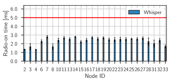
(b) Radio on-time when no signaling packet is disseminated. Whisper achieves a low radio on-time even when no signaling packet is disseminated. In contrast, Whisper (lazy) and Glossy use a fixed timeout mechanism that is set to 5 ms (marked as red line) to turn the radio off in case no packlet has been received. Learning the distance to the source (node 1) allows for energy-efficient channel checks.

Figure 5. Performance of Whisper, Whisper (lazy), Glossy, and Glossy (2b preamble) at 0 dBm in FlockLab in a data dissemination scenario with only a single, fixed sender (diss. fixed). Whisper outperforms Glossy in terms of energy-efficiency during data dissemination as well as when no signaling packet has been sent.

We first compare the performance of Whisper, Whisper (lazy) as well as Glossy and Glossy (2b preamble) in a dissemination scenario with a single, fixed sender (diss. fixed). This scenario corresponds to, e.g., a controller that needs to signal the nodes to stay awake for an unscheduled software update or to disseminate some configuration parameters to all nodes in the network. We find that nodes using Whisper achieve, with respect to Glossy, a comparable or higher reliability and a significantly smaller radio-on time, both with and without data traffic.

Experiments

We run Whisper, Whisper (lazy), “standard” Glossy and Glossy (2b preamble) in the following configuration. We select the node with identifier 1 as the sender. This node is located on the outer edge of the FlockLab testbed, which allows us to obtain a large network diameter. To vary the topology and in particular the number of hops between the sender and the farthest receivers, we use two different transmit powers: -10 dBm and 0 dBm. This results in a network diameter of 3 to 4 and 5 to 6 hops, respectively. Each experiment consists of 10’000 floods and we repeat each experiment 3 times. For Whisper, we further measure the radio-on time over 5’000 slots during which the sender sends no signaling packet. The collected per-node data is averaged over the three independent runs and the standard deviation is plotted as error bars in the figures.

Results

Fig. 5a details – for the case in which the sender disseminates a signaling packet in each slot – the per-node reliability in the upper plot and the per-node radio-on time in the lower plot. While the reliability of Whisper and Whisper (lazy) is comparable or slightly higher than that of Glossy and Glossy (2b preamble), the radio-on time is significantly lower – on average half that of Glossy– for Whisper and Whisper (lazy). Assuming that the protocols are scheduled every second, Whisper has a 50% higher network lifetime than Glossy . Fig. 5a also shows that Whisper and Whisper (lazy) achieve a similar radio-on time. However, with increasing network diameter, the radio-on time of Whisper (lazy) significantly increases compared to Whisper, as shown in Table 2 at -10 dBm.

Fig. 5b shows the per-node radio-on time of Whisper when no signaling packet is sent. The bold, (red) line at 5 ms corresponds to the radio-on time of approaches like Whisper (lazy) or Glossy that – in case of the absence of communication – keep nodes in idle listening for the entire slot. Whisper can save radio-on time by a factor of 2 in this case thanks to the use of direction-aware sampling, which makes nodes switch their radio off at most when the expected reception time of the packlet with counter $c=c_{max}+N_{tx}+1$ has elapsed. This characteristic of Whisper is particularly relevant when nodes must frequently switch on their radios to limit delays in relaying data traffic – yet often no packet is flooded, like in the data prediction scenario of Crystal (18).

Table 2. Summary of evaluation results. Whisper and Whisper (lazy) outperform Glossy in terms of reliability and radio-on time in various scenarios. Nodes using Whisper (lazy) and Glossy use a timeout mechanism to turn the radio off in case they have not intercepted a packlet/packet within a given time. In this evaluation the timeout is set to 5 ms.

Protocol	Scenario	Tx power	Reliability	Radio on	Radio on
				w/ signaling	w/o signaling
		[dBm]	[%]	[ms]	[ms]
	diss. fixed	-10	99.980	2.055	2.546
		0	99.980	1.936	2.474
	diss. fixed	-10	99.817	2.477	5.0
		0	99.983	1.962	5.0
	diss. diff.	-10	99.932	2.175	5.0
		0	99.986	1.865	5.0
	diss. close	-10	99.887	2.438	5.0
		0	99.952	2.129	5.0
	diss. far	-10	99.786	1.626	5.0
		0	99.965	1.540	5.0
	diss. fixed	-10	99.738	4.253	5.0
		0	99.828	3.756	5.0
	diss. fixed	-10	99.616	3.914	5.0
		0	99.767	3.356	5.0
	diss. diff.	-10	98.369	3.805	5.0
		0	98.963	3.351	5.0
	diss. close	-10	99.350	4.071	5.0
		0	99.024	3.932	5.0
	diss. far	-10	98.881	3.680	5.0
		0	98.559	3.721	5.0

4.3. Whisper in dissemination scenarios

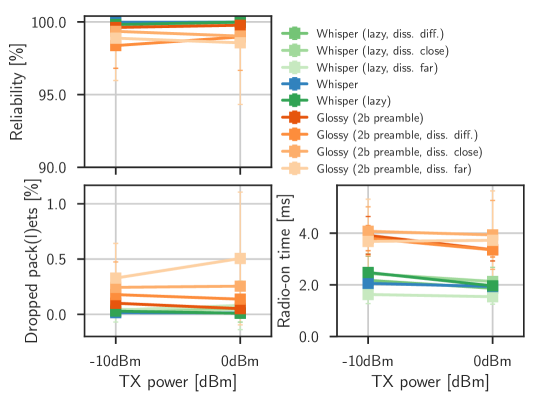
Figure 6. Comparison in dissemination scenarios. Whisper and Whisper (lazy) achieve in all scenarios a two-fold lower radio-on time compared to Glossy. At the same time, they achieve a higher reliability.

To consider the case in which different nodes must disseminate data – possibly even concurrently – we evaluate the performance of Whisper, Whisper (lazy) and Glossy in the three scenarios diss. diff., diss. close, and diss. far (see Table 2). We find that contention for the same slot causes less packet collisions, and thus, results in higher reliability in Whisper and Whisper (lazy) compared to Glossy.

Experiments

We run Whisper, Whisper (lazy) and Glossy consecutively with transmit powers -10 dbm and 0 dBm. In the diss. diff. scenario, each sender – shown in Table 1 – consecutively transmits 1’000 signaling packets before handing over to the next sender. The senders in the diss. close, and diss. far scenarios concurrently transmit signaling packets in every Whisper slot. We execute 10’000 floods in each experiment (i.e., for each protocol) and we run each experiment 3 times.

Results

Fig. 6 shows the network reliability (upper plot, left), radio-on time (lower plot, right) and the percentage of dropped packlets/packets per Whisper/Glossy slot. In all the considered scenarios, Whisper and Whisper (lazy) achieve a higher reliability and a lower radio-on time than Glossy.

The difference in performance is more evident in scenarios with concurrent senders, i.e., diss. close and diss. far. The reason is that interference due to concurrent floods has a stronger impact in Glossy than in Whisper. More precisely, floods from different senders overlap with a slightly different temporal displacement caused by (i) senders not being synchronized within sub-microseconds and (ii) as stated in  (27) “a combination of software, hardware, and signal propagation delays” caused by an increasing number of concurrent transmitters. While (i) affects both Whisper and Glossy to an equal extent, (ii) intensifies for each gap between consecutive transmissions, resulting in a stronger impact on Glossy compared to Whisper. The consequence is that nodes using Glossy drop more packets on average, e.g., 0.5% in diss. far resulting in 1% lower reliability compared to Whisper (lazy).

4.4. Impact of low-level mechanisms

We now investigate the impact of the individual low-level mechanisms used in Whisper. We thereby consider a dissemination scenario with a single, fixed initiator (diss. fixed).

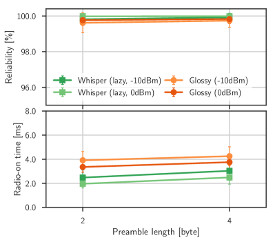
(a) Impact of preamble length. A 4 byte preamble increases the overall reliability by 0.1% while increasing the radio-on time by 20% and 10% for Whisper and Glossy, respectively, compared to a 2 byte preamble.

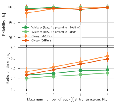
(b) Impact of number of packlet/packet transmissions. Glossy’s radio-on time increases stronger with $N_{tx}$ compared to Whisper’s (lazy, 4b preamble). The reason is the additional packet reception as well as the RX/TX turnaround.

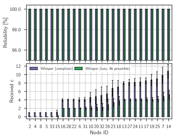
(c) Impact of length field. Colliding lenght fields in Whisper (compliant) have a great impact on the progression speed of the flood.

Figure 7. Impact of low-level mechanisms.

4.4.1. Impact of preamble length

We start by analyzing the effect of the preamble length on the performance of Whisper (lazy) and Glossy. We find that a 2 byte preamble significantly reduces the radio-on time for both protocols while causing a neglibile loss in terms of reliability.

Experiments

We run Whisper (lazy) and Glossy in the diss. fixed scenario using $N_{tx}=3$, preamble length of both 2 bytes and 4 bytes, and transmit powers of -10 dBm and 0 dBm. We execute 10’000 Whisper/Glossy network floods for each protocol and collect data from 3 independent runs.

Results

Fig. 7a shows the network reliability in the upper plot and the achieved radio-on time in the lower plot. One can observe a slight increase in reliability with the 4 byte preamble compared to the 2 byte preamble. Comparing the gray-shadowed results corresponding to $N_{tx}=3$ in Table 3a, the network reliability with a 2 byte preamble drops about 0.1% for all protocols and transmit powers, which corresponds to the loss of 10 packets out of 10,000, on average. The radio-on time, however, increases with the longer preamble by 10% and 20% for Whisper (lazy) and Glossy, respectively, as shown in Fig. 7a. To an almost negligible decrease of reliability, thus, corresponds a significant improvement in terms of radio-on time. This can be explained considering that the preamble and SFD byte are used by receivers to achieve symbol synchronization and to adjust for frequency offsets (40). The length of the preamble, however, only affects transmissions. The receiver starts intercepting a packet as soon as it has found a single preamble byte followed by the SFD. Transmitting a longer preamble is useful to increase the signal-to-noise ratio, and thus, to help the receiver in detecting the preamble and SFD bytes. An increase of the preamble length from 2 to 4 bytes leads, however, to almost negligible improvements, as illustrated above.

4.4.2. Impact of the number of transmissions $N_{tx}$

We now discuss how different values of $N_{tx}$ affect the performances of both Whisper and Glossy. We find that both protocols achieve a similar reliability. However, Whisper (lazy, 4b preamble) has a smaller radio-on time than Glossy and with every $N_{tx}$, the effect on the radio-on time increases stronger in Glossy compared to Whisper (lazy, 4b preamble).

Experiments

We run Whisper (lazy, 4b preamble) and set $N_{tx}=\{2,3,4,5\}$. We use transmit powers -10 dBm and 0 dBm and execute 10’000 Whisper/Glossy network floods for each protocol and collect data from 3 independent runs. We further run “standard” Glossy with a preamble length of 4 byte in the same configuration.

Results

The upper plot of Fig. 7b shows that for different values of $N_{tx}$ Whisper (lazy, 4b preamble) and Glossy achieve a comparable reliability. Apart from minor fluctuations, the reliability increases as $N_{tx}$ increases, as expected. The lower plot in Fig. 7b shows that Whisper outperforms Glossy in terms of radio-on time even with lazy sampling and 4 byte preamble. More precisely, Table 3b shows that in Whisper (lazy, 4b preamble) increasing $N_{tx}$ by 1 causes an increase of the radio-on time of roughly 288 $\mu$s – which corresponds to $T_{packlet}$ for a packlet with a 4 byte preamble and a 1-byte payload. In Glossy the radio on-time increases for each $N_{tx}$ by the duration of one received and one transmitted packet à 288 $\mu$s, the RX/TX turnaround time with 192 $\mu$s and 23 $\mu$s for the software delay. As a consequence, the increase in radio-on time with increasing $N_{tx}$ is more prominent in Glossy than in Whisper.

4.4.3. Impact of collisions due to different length fields

Lastly, we compare Whisper (compliant) with Whisper (lazy, 4b preamble, 14 packlets). We find that collisions caused by the different length fields in Whisper (compliant) have a significant, negative influence on the speed at which a flood can progress.

Experiments

We run Whisper (compliant) with 14 packlets, which results in a signaling packet of 122 bytes. We further run Whisper (lazy, 4b preamble, 14 packlets) and make all nodes stop transmitting their signaling packets simultaneously. The signaling packets in Whisper (compliant) and in Whisper (lazy, 4b preamble, 14 packlets) differ only in the length field of the first packlet. This is the length of the signaling packet in Whisper (compliant) and the length of a packlet in the latter.

Results

Fig. 7c shows the per-node reliability on the upper plot and the received counter $c$ on the lower plot. We find that each node achieves a reliability of 100% for both protocols. This is consistent with the results discussed in the previous Sec. 4.4.2, where we found that the reliability increases with each additionally transmitted packlet. This is also the case when nodes simultaneously stop sending instead of ceasing after $N_{tx}$ transmissions.

The lower plot of Fig. 7c reveals that nodes using Whisper (compliant) receive higher counter values compared to Whisper (lazy, 4b preamble, 14 packlets). This is what causes a slower progression of the flood and is not unexpected given that in Whisper (compliant) (i) nodes drop packlets whose length field is not set correctly, and (ii) the packlets are exposed to collisions due to the different length fields. More precisely, the packlet with $c=0$ is dropped by the nodes in the first hop (nodes with identifiers 2 to 15 in Flocklab), because the length field is not set to the length of a packlet but to the length of the signaling packet. The nodes in the first hop receive packlet $c=1$ and consequently miss $c=2$ due to the RX/TX turnaround. They transmit packlet $c=3$, which collides with the packlet of the sender. Thus, nodes on the second hop (identifiers 16 to 31) successfully receive packlet $c=4$. This procedure continues until the last hop (node with identifier 14) receives packlet $c=11$. In comparison, the same node receives $c=5$ with Whisper (lazy, 4b preamble, 14 packlets). This shows that the flood progresses faster with Whisper (lazy, 4b preamble, 14 packlets), and thus, requires less packlets to be sent in total, which reduces the radio-on time.

Table 3. Summary of low-level mechanisms.

		4b preamble					2b preamble
Protocol	Tx power	$N_{tx}=2$	$=3$	$=4$	$=5$		$N_{tx}=3$
	[dBm]	[%]					[%]
Whisper (lazy)	-10	99.774	99.921	99.672	99.953		99.817
Whisper (lazy)	0	99.985	99.986	99.996	99.998		99.983
Glossy	-10	99.204	99.738	99.870	99.888		99.616
Glossy	0	99.613	99.828	99.649	99.939		99.767

(a) Reliability.

		4 byte preamble					2 byte preamble
Protocol	Tx power	$N_{tx}=2$	$=3$	$=4$	$=5$		$N_{tx}=3$
	[dBm]	[ms]					[ms]
Whisper (lazy)	-10	2.718	3.036	3.587	3.705		2.477
Whisper (lazy)	0	2.118	2.487	2.772	3.109		1.962
Glossy	-10	3.367	4.253	5.303	6.363		3.914
Glossy	0	2.781	3.756	4.834	5.841		3.356

(b) Radio-on time.

5. Evaluating Whisper as wake-up primitive within Crystal

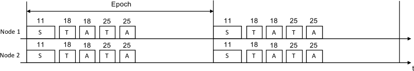
(a) Crystal.

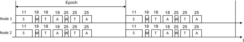
(b) Crystal /w Whisper.

Figure 8. A Crystal epoch with and without Whisper. The (W-), T- and A-slot alternate until the sink node has disseminated a negative-acknowledgment twice during the A-slot. The numbers above the slots denote the channel used for communication. The illustrations are based on Figure 5 in (19).

In the following, we evaluate Whisper used as wake-up primitive in Crystal (18; 19), a recently proposed data collection protocol based on Glossy that targets data prediction scenarios. We show the performance of Crystal and Crystal with integrated Whisper and find that Whisper increases the network lifetime by a factor of 2.3 compared to “standard” Crystal.

Crystal and Crystal with Whisper

In the following, we briefly describe the operation of Crystal and afterwards how Whisper is incorporated in Crystal.

Crystal uses Glossy-floods to let nodes transmit data to a sink node. When the sink node has received a data packet, it acknowledges its reception. Otherwise, it disseminates a negative-acknowledgment. The transmit (T) and acknowledgment (A) slots alternate until the sink has disseminated a negative-acknowledgment twice. After the second negative-acknowledgment, the nodes turn their radio off. Crystal runs periodically and organizes its operations in epochs. Fig. 8a shows an example of a Crystal epoch. Each epoch starts with a synchronization (S) slot in which the nodes re-synchronize to the sink node. After the synchronization slot follow the T- and A-slots as described above. To increase resilience against interference, Crystal integrates a channel hopping mechanism. The numbers above the communication slots in Fig. 8a indicate the channel at which the nodes communicate. In particular, each TA-pair uses the same channel.

The sink node always disseminates packets in the S- and A-slot. However, there is infrequent communication in the T-slot. For example, in Crystal’s temperature prediction scenario, there is no data dissemination in over 80% of the T-slots. However, the duration of the T-slot must be sufficiently long to support the packet size that is required by the application. As a consequence, the nodes consume unnecessary energy. To reduce the idle listening time when no data communication is needed, and thus, to reduce the energy consumption, Whisper can be integrated into Crystal as wake-up primitive. Fig. 8b shows Crystal with Whisper. Whisper (W) runs before each T-slot. A node that has data to share, transmits a signaling packet in the Whisper slot. The packlets in the signaling packet only carry the counter $c$ as payload, and thus, the data field has a length of zero. Nodes that intercept a packlet turn their radio on in the T-slot, otherwise they keep the radio turned off until the following A-slot. In this setting, Whisper relies on the synchronization and channel hopping mechanisms from Crystal. More precisely, Crystal initiates the start of the Whisper slot and also provides the communication channel, which is the same as used for the TA-slots.

Experiments

Table 4. Crystal’s configuration parameters.

Tx power	$N_{S}$	$N_{T}$	$N_{A}$		$W_{S}$	$W_{T}$	$W_{A}$
[dBm]	[#]	[#]	[#]		[ms]	[ms]	[ms]
0	3	2	3		10	9	7
-10	4	3	4		14	14	12

In this experiment, we measure the duty cycle and the achieved reliability. In particular, the duty cycle is the averaged per-node duty cycle that is the ratio of the sum of the radio-on time for all slots during an epoch and the duration of the epoch. The reliability indicates how many nodes that have transmitted an update in the current epoch also received an acknowledgment from the sink. Thus, the measured reliability includes the packet reception rates of the T-slot, the A-slot, and when used, also the Whisper (W)-slot.

Since Crystal is a collection protocol, we run Whisper using a “reversed” direction-aware sampling strategy, henceforth called Whisper (coll.). Thereby, the nodes must know their distance in hops to the sink, which they can learn through a short initialization phase. The nodes can then derive their position in the collection tree by subtracting their distance in hops to the root from the network diameter. We use Crystal’s bootstrapping period – which lasts 10 epochs – as initialization phase for Whisper to let the nodes learn their position in the network tree. We run Crystal with an epoch of 1.5 s and a data payload of 20 bytes. We use the default number of retransmissions $N$ for the different slots and transmit powers, given in (18) and summarized in Table 4. As also shown in the table, we further use the default duration $W$ for the S- and A-slots. However, since we increase the payload, we also adjust the duration for the T-slot. We run Crystal in FlockLab, with node 1 as sink, and with updates $u=0$, $u=2$, and $u=5$. An update $u=X$ implies that among the 27 nodes in FlockLab, there are X events (or data packets) to share during a specific epoch. Crystal with $u=0$ indicates that no message is transmitted in the T-slots, and thus, in this case we measure the idle listening time of Crystal. More precisely, $u=0$ indicates the minimal power consumption, and we, thus, use it as baseline for other update configurations. After running Crystal 3 times for 60 minutes, we repeat the experiments with Crystal using Whisper (coll.).

Results

Fig. 9 shows the duty cycle in the upper plot and the reliability in the lower plot. We find that Whisper reduces the duty cycle by a factor of two for all updates $u$. Considering only the energy consumption during communication (i.e., 20 mA) and assuming a battery with a capacity of 2000 mAh, Crystal with Whisper increases the nodes’ lifetime by a factor of 2.3 compared to “standard” Crystal (278 days vs. 119 days of lifetime) in this experiment. The factor of how much Whisper increases the network lifetime depends on the size of the packets sent in the T-slot as well as the number of retransmissions. A large packet requires a long duration of the T-slot compared to short packets. The longer the duration of the T-slot, the higher is the gain in terms of energy-efficiency that Whisper is able to achieve.
However, one can also observe that Crystal with Whisper has a lower reliability compared to “standard” Crystal (e.g., 95.7% vs. 98.4% at -10 dBm with $u=5$). Indeed, when the sink misses a packlet in a Whisper slot, it keeps its radio turned off during the T-slot and thus, also misses the data packet. Thus, Whisper requires high reliability when used as wake-up service. New sampling strategies or a higher value for $N_{tx}$, as shown in Section 4.4.2, can help to increase Whisper’s reliability.

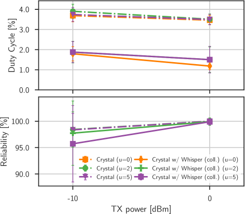
Figure 9. Impact of Whisper on Crystal. Whisper halves the duty cycle of Crystal. However, a missed packlet in Whisper also impacts the reliability of Crystal.

6. Related work

The overall architecture of Whisper builds on the concepts introduced by Glossy. The novel design elements that we introduce – in particular packlets and direction-aware sampling – make Whisper significantly more efficient than Glossy, especially for small payload sizes. Whisper’s superior performance is obtained by completely eliminating gaps between consecutive, synchronous transmissions.

Lim et al. (24) modify Glossy so that a packet is transmitted multiple times after a single reception. Consecutive packets are, however, not sent back-to-back as in Whisper but have gaps between them. This is because they are transmitted as individual packets and, thus, the radio must still perform a turnaround even between consecutive transmissions. This increases the overall transmit time and strongly limits the use of sampling strategies as introduced in Whisper. Furthermore, due to the instability of the DCO, the alignment of concurrently transmitted packets decreases quickly with the number of packets. In Whisper, instead, the use of Flock (7) and the concept of packlets guarantee that transmissions are precisely aligned.

Approaches that exploit scheduled Glossy floods to provide high-level protocols – e.g., LWB (15), Crystal (18; 19), or LaneFlood (6) – could replace Glossy with Whisper to achieve a more efficient operation. Other, more complex protocols like Splash (9) or Pando (10) could also benefit from integrating Whisper’s design in their architecture.

Several authors proposed protocols to use some form of frequency diversity to make synchronous transmissions more robust to interference. These include full-fledged protocols like Splash (9) or Pando (10) but also improved versions of Glossy like the one proposed by Sommer and Pignolet (34). While we have not yet implemented the use of multiple channels within Whisper, this is part of our future work.

Other approaches related to Whisper are those that provide – or can be used to implement – a network-wide wake-up service. Some basic techniques like Low-Power Listening (31) or Backcast (12) have been successfully used in Medium Access Control protocols to schedule nodes’ rendezvous (31; 8; 28; 11). They are, however, contention-based approaches and are inherently less performing – both in terms of reliability and latency – than approaches based on synchronous transmissions.

Lastly, protocols that exploit wake-up radios – like, e.g., Zippy (36), ALBA-WUR (35), or the approach proposed in (25) – are orthogonal to ours because they rely on specialized hardware to be available on network nodes.

7. Conclusions

This paper introduces Whisper, a novel primitive to provide quick and reliable network floods. Whisper exploits synchronous transmissions as in Glossy but eliminates any gap between consecutive transmissions of the packet to flood. This allows Whisper to halve the radio-on time of the nodes with respect to Glossy while maintaining a comparable or even higher reliability – as demonstrated through our experiments on the FlockLab testbed. Whisper can be used as a stand-alone primitive to disseminate small values or be integrated in place of Glossy in protocols like, e.g., Crystal (18). The source code of Whisper is publicly available at http://github.com/martinabr/whisper.

Appendix A: Theoretical radio-on time for large payloads

Table 5 shows the radio-on time for Glossy, Whisper, and Whisper (lazy) for different payload sizes and network diameters. The cells highlighted in gray indicate when the radio-on time of Whisper (lazy) exceeds the one of Glossy. Thus, the non-highlighted cells in the columns for Whisper and Whisper (lazy) show when they have achieved a lower radio-on time than Glossy.

Table 5. Theoretical radio-on time of Glossy, Whisper, and Whisper (lazy) for different payload sizes and hop counts. Whisper has a lower radio-on time compared to Glossy. However, depending on the payload size and the number of hops, the radio-on time for Whisper (lazy) may exceed the one of Glossy (the gray marked cells). The values include a RX/TX turnaround time of 192 $\mu$s for Glossy but neglect the software delay.

Payload	Glossy						Whisper						Whisper (lazy)
size	Hop 1	2	3	4	5	6	Hop 1	2	3	4	5	6	Hop 1	2	3	4	5	6
[byte]	[ms]	[ms]	[ms]	[ms]	[ms]	[ms]	[ms]	[ms]	[ms]	[ms]	[ms]	[ms]	[ms]	[ms]	[ms]	[ms]	[ms]	[ms]
1	2.30	2.72	3.14	3.55	3.97	4.38	1.12	1.34	1.34	1.34	1.34	1.34	1.12	1.57	2.02	2.46	2.91	3.36
2	2.50	2.94	3.39	3.84	4.29	4.74	1.28	1.54	1.54	1.54	1.54	1.54	1.28	1.79	2.30	2.82	3.33	3.84
3	2.69	3.17	3.65	4.13	4.61	5.09	1.44	1.73	1.73	1.73	1.73	1.73	1.44	2.02	2.59	3.17	3.74	4.32
4	2.88	3.39	3.90	4.42	4.93	5.44	1.60	1.92	1.92	1.92	1.92	1.92	1.60	2.24	2.88	3.52	4.16	4.80
5	3.07	3.62	4.16	4.70	5.25	5.79	1.76	2.11	2.11	2.11	2.11	2.11	1.76	2.46	3.17	3.87	4.58	5.28
6	3.26	3.84	4.42	4.99	5.57	6.14	1.92	2.30	2.30	2.30	2.30	2.30	1.92	2.69	3.46	4.22	4.99	5.76
7	3.46	4.06	4.67	5.28	5.89	6.50	2.08	2.50	2.50	2.50	2.50	2.50	2.08	2.91	3.74	4.58	5.41	6.24
8	3.65	4.29	4.93	5.57	6.21	6.85	2.24	2.69	2.69	2.69	2.69	2.69	2.24	3.14	4.03	4.93	5.82	6.72
9	3.84	4.51	5.18	5.86	6.53	7.20	2.40	2.88	2.88	2.88	2.88	2.88	2.40	3.36	4.32	5.28	6.24	7.20
10	4.03	4.74	5.44	6.14	6.85	7.55	2.56	3.07	3.07	3.07	3.07	3.07	2.56	3.58	4.61	5.63	6.66	7.68
11	4.22	4.96	5.70	6.43	7.17	7.90	2.72	3.26	3.26	3.26	3.26	3.26	2.72	3.81	4.90	5.98	7.07	8.16
12	4.42	5.18	5.95	6.72	7.49	8.26	2.88	3.46	3.46	3.46	3.46	3.46	2.88	4.03	5.18	6.34	7.49	8.64
13	4.61	5.41	6.21	7.01	7.81	8.61	3.04	3.65	3.65	3.65	3.65	3.65	3.04	4.26	5.47	6.69	7.90	9.12
14	4.80	5.63	6.46	7.30	8.13	8.96	3.20	3.84	3.84	3.84	3.84	3.84	3.20	4.48	5.76	7.04	8.32	9.60
15	4.99	5.86	6.72	7.58	8.45	9.31	3.36	4.03	4.03	4.03	4.03	4.03	3.36	4.70	6.05	7.39	8.74	10.08
16	5.18	6.08	6.98	7.87	8.77	9.66	3.52	4.22	4.22	4.22	4.22	4.22	3.52	4.93	6.34	7.74	9.15	10.56
17	5.38	6.30	7.23	8.16	9.09	10.02	3.68	4.42	4.42	4.42	4.42	4.42	3.68	5.15	6.62	8.10	9.57	11.04
18	5.57	6.53	7.49	8.45	9.41	10.37	3.84	4.61	4.61	4.61	4.61	4.61	3.84	5.38	6.91	8.45	9.98	11.52
19	5.76	6.75	7.74	8.74	9.73	10.72	4.00	4.80	4.80	4.80	4.80	4.80	4.00	5.60	7.20	8.80	10.40	12.00
20	5.95	6.98	8.00	9.02	10.05	11.07	4.16	4.99	4.99	4.99	4.99	4.99	4.16	5.82	7.49	9.15	10.82	12.48
21	6.14	7.20	8.26	9.31	10.37	11.42	4.32	5.18	5.18	5.18	5.18	5.18	4.32	6.05	7.78	9.50	11.23	12.96
22	6.34	7.42	8.51	9.60	10.69	11.78	4.48	5.38	5.38	5.38	5.38	5.38	4.48	6.27	8.06	9.86	11.65	13.44
23	6.53	7.65	8.77	9.89	11.01	12.13	4.64	5.57	5.57	5.57	5.57	5.57	4.64	6.50	8.35	10.21	12.06	13.92
24	6.72	7.87	9.02	10.18	11.33	12.48	4.80	5.76	5.76	5.76	5.76	5.76	4.80	6.72	8.64	10.56	12.48	14.40
25	6.91	8.10	9.28	10.46	11.65	12.83	4.96	5.95	5.95	5.95	5.95	5.95	4.96	6.94	8.93	10.91	12.90	14.88
26	7.10	8.32	9.54	10.75	11.97	13.18	5.12	6.14	6.14	6.14	6.14	6.14	5.12	7.17	9.22	11.26	13.31	15.36
27	7.30	8.54	9.79	11.04	12.29	13.54	5.28	6.34	6.34	6.34	6.34	6.34	5.28	7.39	9.50	11.62	13.73	15.84
28	7.49	8.77	10.05	11.33	12.61	13.89	5.44	6.53	6.53	6.53	6.53	6.53	5.44	7.62	9.79	11.97	14.14	16.32
29	7.68	8.99	10.30	11.62	12.93	14.24	5.60	6.72	6.72	6.72	6.72	6.72	5.60	7.84	10.08	12.32	14.56	16.80
30	7.87	9.22	10.56	11.90	13.25	14.59	5.76	6.91	6.91	6.91	6.91	6.91	5.76	8.06	10.37	12.67	14.98	17.28
31	8.06	9.44	10.82	12.19	13.57	14.94	5.92	7.10	7.10	7.10	7.10	7.10	5.92	8.29	10.66	13.02	15.39	17.76
32	8.26	9.66	11.07	12.48	13.89	15.30	6.08	7.30	7.30	7.30	7.30	7.30	6.08	8.51	10.94	13.38	15.81	18.24
33	8.45	9.89	11.33	12.77	14.21	15.65	6.24	7.49	7.49	7.49	7.49	7.49	6.24	8.74	11.23	13.73	16.22	18.72
34	8.64	10.11	11.58	13.06	14.53	16.00	6.40	7.68	7.68	7.68	7.68	7.68	6.40	8.96	11.52	14.08	16.64	19.20
35	8.83	10.34	11.84	13.34	14.85	16.35	6.56	7.87	7.87	7.87	7.87	7.87	6.56	9.18	11.81	14.43	17.06	19.68
36	9.02	10.56	12.10	13.63	15.17	16.70	6.72	8.06	8.06	8.06	8.06	8.06	6.72	9.41	12.10	14.78	17.47	20.16
37	9.22	10.78	12.35	13.92	15.49	17.06	6.88	8.26	8.26	8.26	8.26	8.26	6.88	9.63	12.38	15.14	17.89	20.64
38	9.41	11.01	12.61	14.21	15.81	17.41	7.04	8.45	8.45	8.45	8.45	8.45	7.04	9.86	12.67	15.49	18.30	21.12
$\cdots$
124	25.92	30.27	34.62	38.98	43.33	47.68	20.8	24.96	24.96	24.96	24.96	24.96	20.8	29.12	37.44	45.76	54.08	62.4
125	26.11	30.5	34.88	39.26	43.65	48.03	20.96	25.15	25.15	25.15	25.15	25.15	20.96	29.34	37.73	46.11	54.5	62.88

References

- (1)
- Arago Systems (2011) Arago Systems. 2011. WiSMote datasheet. (2011).
- Atmel (2009) Atmel. 2009. AT86RF231 datasheet. (2009).
- Atmel (2016) Atmel. 2016. AT86RF215 datasheet. (2016).
- Boano et al. (2014) Carlo Alberto Boano, Marco Zúñiga, James Brown, Utz Roedig, Chamath Keppitiyagama, and Kay Römer. 2014. TempLab: A Testbed Infrastructure to Study the Impact of Temperature on Wireless Sensor Networks. In Proceedings of the Conference on Information Processing in Sensor Networks (ACM/IEEE IPSN). 95–106.
- Brachmann et al. (2016) Martina Brachmann, Olaf Landsiedel, and Silvia Santini. 2016. Concurrent Transmissions for Communication Protocols in the Internet of Things. In Proceedings of the Conference on Local Computer Networks (IEEE LCN). 406–414.
- Brachmann et al. (2017) Martina Brachmann, Olaf Landsiedel, and Silvia Santini. 2017. Keep the Beat: On-The-Fly Clock Offset Compensation for Synchronous Transmissions in Low-Power Networks. In Proceedings of the Conference on Local Computer Networks (IEEE LCN). 303–311.
- Buettner et al. (2006) Michael Buettner, Gary V. Yee, Eric Anderson, and Richard Han. 2006. X-MAC: A Short Preamble MAC Protocol for Duty-cycled Wireless Sensor Networks. In Proceedings of the Conference on Embedded Networked Sensor Systems (ACM SenSys). 307–320.
- Doddavenkatappa et al. (2013) Manjunath Doddavenkatappa, Mun Choon Chan, and Ben Leong. 2013. Splash: Fast Data Dissemination with Constructive Interference in Wireless Sensor Networks. In Proceedings of the Symposium on Networked Systems Design & Implementation (USENIX NSDI). 269–282.
- Du et al. (2015) Wan Du, Jansen Christian Liando, Huanle Zhang, and Mo Li. 2015. When Pipelines Meet Fountain: Fast Data Dissemination in Wireless Sensor Networks. In Proceedings of the Conference on Embedded Networked Sensor Systems (ACM SenSys). 365–378.
- Dutta et al. (2012) Prabal Dutta, Stephen Dawson-Haggerty, Yin Chen, Chieh-Jan Mike Liang, and Andreas Terzis. 2012. A-MAC: A Versatile and Efficient Receiver-initiated Link Layer for Low-power Wireless. ACM Transactions on Sensor Networks 8 (2012), 1–29. Issue 4.
- Dutta et al. (2008) Prabal Dutta, Răzvan Musăloiu-E., Ion Stoica, and Andreas Terzis. 2008. Wireless ACK Collisions Not Considered Harmful. In Proceedings of the Workshop on Hot Topics in Networks (ACM HotNets). 1–6.
- El-Hoiydi and Decotignie (2004) Amre El-Hoiydi and Jean Dominique Decotignie. 2004. WiseMAC: An ultra low power MAC protocol for the downlink of infrastructure Wireless Sensor networks. In Proceedings of the Symposium on Computers and Communications (IEEE ISCC). 244–251.
- Escobar et al. (2018) Antonio Escobar, Fernando Moreno, Borja Saez, Antonio J. Cabrera, Javier Garcia-Jimenez, Francisco J. Cruz, Unai Ruiz, Angel Corona, Jirka Klaue, and Divya Tati. 2018. Competition: BigBangBus. In Proceedings of the European Conference on Wireless Sensor Networks (EWSN). 213–214.
- Ferrari et al. (2012) Federico Ferrari, Marco Zimmerling, Luca Mottola, and Lothar Thiele. 2012. Low-power wireless bus. In Proceedings of the Conference on Embedded Networked Sensor Systems (ACM SenSys). 1–14.
- Ferrari et al. (2011) Federico Ferrari, Marco Zimmerling, Lothar Thiele, and Olga Saukh. 2011. Efficient network flooding and time synchronization with Glossy. In Proceedings of the Conference on Information Processing in Sensor Networks (ACM/IEEE IPSN). 73–84.
- IEEE Computer Society (2016) IEEE Computer Society. 2016. IEEE Standard for Low-Rate Wireless Networks. (2016).
- Istomin et al. (2016) Timofei Istomin, Amy L. Murphy, Gian Pietro Picco, and Usman Raza. 2016. Data Prediction + Synchronous Transmissions = Ultra-low Power Wireless Sensor Networks. In Proceedings of the Conference on Embedded Networked Sensor Systems (ACM SenSys). 83–95.
- Istomin et al. (2018) Timofei Istomin, Matteo Trobinger, Amy L. Murphy, and Gian Pietro Picco. 2018. Interference-Resilient Ultra-Low Power Aperiodic Data Collection. In Proceedings of the Conference on Information Processing in Sensor Networks (ACM/IEEE IPSN). 84–95.
- König and Wattenhofer (2016) Michael König and Roger Wattenhofer. 2016. Maintaining Constructive Interference Using Well-Synchronized Sensor Nodes. In Proceedings of the Conference Distributed Computing in Sensor Systems (DCOSS). 206–215.
- Landsiedel et al. (2013) Olaf Landsiedel, Federico Ferrari, and Marco Zimmerling. 2013. Chaos: Versatile and Efficient All-to-All Data Sharing and In-Network Processing at Scale. In Proceedings of the Conference on Embedded Networked Sensor Systems (ACM SenSys). 1–14.
- Liang et al. (2010) Chieh-Jan Mike Liang, Nissanka Bodhi Priyantha, Jie Liu, and Andreas Terzis. 2010. Surviving Wi-fi Interference in Low Power ZigBee Networks. In Proceedings of the Conference on Embedded Networked Sensor Systems (ACM SenSys). 309–322.
- Lim et al. (2013) Roman Lim, Federico Ferrari, Marco Zimmerling, Christoph Walser, Philipp Sommer, and Jan Beutel. 2013. FlockLab: A Testbed for Distributed, Synchronized Tracing and Profiling of Wireless Embedded Systems. In Proceedings of the Conference on Information Processing in Sensor Networks (ACM/IEEE IPSN). 153–166.
- Lim et al. (2017) Roman Lim, Reto Da Forno, Felix Sutton, and Lothar Thiele. 2017. Competition: Robust Flooding using Back-to-Back Synchronous Transmissions with Channel-Hopping. In Proceedings of the European Conference on Wireless Sensor Networks (EWSN). 270–271.
- Liu et al. (2016) Xuefeng Liu, Jiannong Cao, Shaojie Tang, and Jiaqi Wen. 2016. Enabling Reliable and Network-Wide Wakeup in Wireless Sensor Networks. IEEE Transactions on Wireless Communications 15 (2016), 2262–2275. Issue 3.
- Ma et al. (2018) Xiaoyuan Ma, Peilin Zhang, Weisheng Tang, Xin Li, Wangji He, Fuping Zhang, Jianming Wei, and Oliver Theel. 2018. Competition: Using Enhanced OFCOIN to Monitor Multiple Concurrent Events under Adverse Conditions. In Proceedings of the European Conference on Wireless Sensor Networks (EWSN). 211–212.
- Mohammad et al. (2017) Mobashir Mohammad, Manjunath Doddavenkatappa, and Mun Choon Chan. 2017. Improving Performance of Synchronous Transmission-Based Protocols Using Capture Effect over Multichannels. ACM Transactions on Sensor Networks 13 (2017), 1–26. Issue 2.
- Moss and Levis (2008) David Moss and Philip Levis. 2008. BoX-MACs: Exploiting Physical and Link Layer Boundariesin Low-Power Networking. Technical Report. 1–12 pages.
- Nahas and Landsiedel (2018) Beshr Al Nahas and Olaf Landsiedel. 2018. Competition: Aggressive Synchronous Transmissions with In-network Processing for Dependable All-to-All Communication. In Proceedings of the European Conference on Wireless Sensor Networks (EWSN). 209–210.
- Olimex Ltd. (2013) Olimex Ltd. 2013. MSP430-CCRF development board. (2013). User’s manual.
- Polastre et al. (2004) Joseph Polastre, Jason Hill, and David Culler. 2004. Versatile Low Power Media Access for Wireless Sensor Networks. In Proceedings of the Conference on Embedded Networked Sensor Systems (ACM SenSys). 95–107.
- Saha and Chan (2017) Sudipta Saha and Mun Choon Chan. 2017. Design and Application of a Many-to-One Communication Protocol. In Proceedings of the Conference on Computer Communications (IEEE INFOCOM). 1–9.
- Semtech (2015) Semtech. 2015. SX1211 datasheet. (2015).
- Sommer and Pignolet (2016) Philipp Sommer and Yvonne-Anne Pignolet. 2016. Competition: Dependable Network Flooding Using Glossy with Channel-Hopping. In Proceedings of the European Conference on Wireless Sensor Networks (EWSN). 303–303.
- Spenza et al. (2015) Dora Spenza, Michele Magno, Stefano Basagni, Luca Benini, Mario Paoli, and Chiara Petrioli. 2015. Beyond Duty Cycling: Wake-up Radio with Selective Awakenings for Long-lived Wireless Sensing Systems. In Proceedings of the Conference on Computer Communications (IEEE INFOCOM). 522–530.
- Sutton et al. (2015) Felix Sutton, Bernhard Buchli, Jan Beutel, and Lothar Thiele. 2015. Zippy: On-Demand Network Flooding. In Proceedings of the Conference on Embedded Networked Sensor Systems (ACM SenSys). 45–58.
- Texas Instruments (2007) Texas Instruments. 2007. CC2520 datasheet. (2007).
- Texas Instruments (2011) Texas Instruments. 2011. MSP430F1611 datasheet. (2011).
- Texas Instruments (2013a) Texas Instruments. 2013a. CC1101 datasheet. (2013).
- Texas Instruments (2013b) Texas Instruments. 2013b. CC2420 datasheet. http://www.ti.com/product/CC2420/. (2013).
- Trobinger et al. (2018) Matteo Trobinger, Timofei Istomin, Amy L. Murphy, and Gian Pietro Picco. 2018. Competition: CRYSTAL Clear: Making Interference Transparent. In Proceedings of the European Conference on Wireless Sensor Networks (EWSN). 217–218.
- Yuan and Hollick (2013) Dingwen Yuan and Matthias Hollick. 2013. Let’s Talk Together: Understanding Concurrent Transmission in Wireless Sensor Networks. In Proceedings of the Conference on Local Computer Networks (IEEE LCN). 219–227.
- Yuan et al. (2014) Dingwen Yuan, Michael Riecker, and Matthias Hollick. 2014. Making ’Glossy’ Networks Sparkle: Exploiting Concurrent Transmissions for Energy Efficient, Reliable, Ultra-Low Latency Communication in Wireless Control Networks. In Proceedings of the European Conference on Wireless Sensor Networks (EWSN). 133–149.