NuSTAR observations of heavily obscured Swift/BAT AGN: constraints on the Compton-thick AGN fraction

The evolution of the accretion history of the Universe has been studied in unprecedented detail owing to recent X-ray surveys performed by Chandra and XMM-Newton. A missing piece of information is the most heavily obscured or Compton-thick AGN which evade detection even in X-ray surveys owing to their extreme hydrogen column densities which exceed $\rm 10^{24}cm^{-2}$. Recently, the all-sky hard X-ray survey performed by Swift/BAT brought a breakthrough allowing the detection of many of these AGN. This is because of its very high energy bandpass ($\rm 14-195$ keV) which helps to minimise attenuation effects. In our previous work, we have identified more than 50 candidate Compton-thick AGN in the local Universe, corresponding to an observed fraction of about 7% of the total AGN population. This number can be converted to the intrinsic Compton-thick AGN number density, only if we know their exact selection function. This function sensitively depends on the form of the Compton-thick AGN spectrum, that is the energy of their absorption turnover, photon-index and its cut-off energy at high energies, as well as the strength of the reflection component on the matter surrounding the nucleus. For example, the reflection component at hard energies 20-40 keV antagonises the number density of missing Compton-thick AGN in the sense that the stronger the reflection the easier these sources are detected in the BAT band. In order to constrain their number density, we analyse the spectra of 19 Compton-thick AGN which have been detected with Swift/BAT and have been subsequently observed with NuSTAR in the 3-80 keV band. We analyse their X-ray spectra using the MYTORUS models of Murphy and Yaqoob which properly take into account the Compton scattering effects. These are combined with physically motivated Comptonisation models which accurately describe the primary coronal X-ray emission. We derive absorbing column densities which are consistent with those derived by the previous Swift/BAT analyses. We estimate the coronal temperatures to be roughly between 25 and 80 keV corresponding to high energy cut-offs roughly between 75 and 250 keV. Furthermore, we find that the majority of our AGN lacks a strong reflection component in the 20-40 keV band placing tighter constraints on the intrinsic Compton-thick AGN fraction. Combining these results with our X-ray background synthesis models, we estimate a Compton-thick AGN fraction in the local Universe of $\approx 20\pm 3$ % relative to the type-II AGN population .

1 Introduction

The vast majority of galaxies contain a supermassive black hole in their centres (e.g. Ferrarese & Merritt, 2000). A fraction of these emit copious amounts of radiation as in-falling matter forms an accretion disk around the black hole. These Active Galactic Nuclei (AGN) constitute at least half of the galaxy population (Ho et al., 1997a, b). The majority of AGN are covered by veils of dust and gas (e.g. Ricci et al. 2017) which probably have a toroidal form (Wada et al., 2009). In most cases this obscuring screen can obliterate the optical emission and reradiate in the IR. X-rays can more easily penetrate these obscuring screens. However, in the most extreme obscuration even the X-ray radiation can be blocked. These are the Compton-thick AGN having column densities exceeding $\rm 10^{24}$ $\rm cm^{-2}$. In this case, the X-rays are Compton scattered on the free electrons of the obscuring screen. As these heavily obscured AGN represent the evasive side of the accretion history of the Universe, it is of primary importance to detect them. However, the methods employed to constrain their number appear to give diverging results.

The most commonly used method is that of X-ray background synthesis models. The spectrum of the X-ray background, that is the integrated X-ray light produced by all X-ray sources in the history of the Universe, presents a peak at 20-30 keV as measured by the HEAO-1, XMM-Newton, BeppoSAX and the INTEGRAL missions (e.g. Gruber et al., 1999; Frontera et al., 2007; Churazov et al., 2007; Moretti et al., 2009). X-ray background synthesis models attempt to reconstruct the spectrum of the X-ray background using the AGN luminosity function, together with a model for the AGN X-ray spectrum. These models have been pioneered by Comastri et al. (1995) and were later refined by Gilli et al. (2007), Treister et al. (2009), Draper & Ballantyne (2009), Akylas et al. (2012), Vasudevan et al. (2013), Ueda et al. (2014), Esposito & Walter (2016). In order to reproduce the hump of the X-ray background, a significant number of Compton-thick AGN is necessary. However, their fraction remains uncertain with figures ranging roughly between 10 and 50 %. This discrepancy is attributed mainly to the fact that there is a degeneracy between the required fraction of Compton-thick AGN and the strength of the total AGN population reflection component. This reflection component originates from scattering and subsequent absorption of the X-ray radiation on surrounding cold material (e.g. George & Fabian, 1991) and results to the flattening of the observed AGN spectrum. The higher the AGN population reflection component the lower the number of Compton-thick AGN required. Interestingly enough, the reflection component strength does not refer to the Compton-thick AGN but to the average reflection component of the total AGN population.

Recently, attention has shifted to the direct detection of Compton-thick AGN using X-ray spectroscopy. The sensitive observations performed with Chandra and XMM-Newton allowed the detection of many faint candidate Compton-thick AGN in the 2-10 keV band mainly in the Chandra Deep Field South area (e.g. Georgantopoulos et al., 2013; Brightman et al., 2014; Buchner et al., 2015) resulting in the derivation of the Compton-thick AGN luminosity function and its evolution. Additional studies have focused on the ultra-hard band above 10 keV where the X-ray attenuation is less severe. The Niel Gehrels Swift, INTEGRAL and NuSTAR missions which operate in this band, readily provide this possibility. The BAT hard X-ray instrument onboard Niel Gehrels Swift is continuously performing an all sky survey in the $14-195$ keV band. As it does not carry imaging X-ray optics it can probe flux limits of only a few times $10^{-12}$ $\rm erg\leavevmode\nobreak\ cm^{-2}\leavevmode\nobreak\ s^{-1}$. Ricci et al. (2015) and Akylas et al. (2016) analysed the X-ray spectra of 688 candidate AGN in the 70-month BAT all-sky survey (Baumgartner et al., 2013). Fitting the X-ray spectra using Bayesian statistics, Akylas et al. (2016) find about 50 Compton-thick AGN candidates in overall agreement with the results of Ricci et al. (2015). The observed fraction of Compton-thick AGN amounts to about 7% of the total AGN population. This number can be extrapolated to the intrinsic fraction of Compton-thick AGN, only by knowing the exact X-ray spectrum of Compton-thick AGN i.e. their selection function. Akylas et al. (2016) find that the intrinsic fraction of Compton-thick AGN, in the local Universe, is between 10 and 30% assuming a reflection component which contributes between 0 and 5% to the total 2-10 keV flux. These estimates are in good agreement with the estimates of Ricci et al. (2015), Burlon et al. (2011) and Malizia et al. (2009). The advantage of the above direct methods is that only knowledge of the X-ray spectrum of Compton-thick AGN is required instead of the average AGN population.

In this paper, we present an X-ray spectral analysis of the Compton-thick AGN in Akylas et al. (2016) which have publicly available NuSTAR spectra. The imaging X-ray optics of NuSTAR (Harrison et al., 2013) allow the derivation of excellent quality spectra. These are used to constrain with the highest accuracy yet, the fraction of Compton-thick AGN in the local Universe. We adopt $\rm H_{o}=75\,km\,s^{-1}\,Mpc^{-1}$, $\rm\Omega_{M}=0.3$, and $\Omega_{\Lambda}=0.7$ throughout the paper.

2 The X-ray Sample & data

2.1 BAT

The Niel Gehrels Swift gamma-ray burst (GRB) observatory (Gehrels et al., 2004) was launched in November 2004 and has been continually observing the hard X-ray ($\rm 14-195$ keV) sky with the Burst Alert Telescope (BAT). BAT is a large, coded-mask telescope optimised to detect transient GRBs and is designed with a very wide field-of-view of $\sim$ 60$\times$100 degrees. Niel Gehrel Swift’s observation strategy is to observe targets with the narrow field-of-view X-ray telescope (XRT), in the $\rm 0.3-10$ keV band until a new GRB is discovered by BAT, at which time Niel Gehrel Swift automatically slews to the new GRB to follow up with the narrow field instruments until the X-ray afterglow is below the XRT detection limit. Baumgartner et al. (2013) presented the catalogue of sources detected in 70 months of observations with BAT. The BAT 70 month survey has detected 1171 hard X-ray sources down to a flux level of $\rm 10^{-11}erg\leavevmode\nobreak\ cm^{-2}\leavevmode\nobreak\ s^{-1}$. The majority of these sources are AGN.

Akylas et al. (2016) analysed the X-ray spectra of these sources employing Bayesian statistics. They considerd 688 sources classified according to the NASA/IPAC Extragalactic Database in the following types: (i) 111 galaxies, (ii) 292 Seyfert I (Sy 1.0- 1.5), (iii) 262 Seyfert II (Sy 1.7-2.0), and (iv) 23 sources of type other AGN. Radio-loud AGN have been excluded since their X-ray emission might be dominated by the jet component. QSOs have been also excluded from the analysis since the fraction of highly absorbed sources within this population is negligible. They have combined the BAT with the XRT data (0.3-10 keV) at softer energies adopting a Bayesian approach to fit the data using Markov chains. This allows us to consider all sources as potential Compton-thick candidates at a certain level of probability. 53 sources present a non-zero probability of being Compton-thick corresponding to 40 effective Compton-thick sources. These represent 7% of the sample in excellent agreement with the figure reported in Ricci et al. (2015) and Burlon et al. (2011). Out of these, 38 sources have a probability of more than 70% being Compton-thick.

2.2 NuSTAR

The Nuclear Spectroscopic Telescope Array, NuSTAR, (Harrison et al., 2013) launched in June 2012, is the first orbiting X-ray observatory which focuses light at high energies (E $>$ 10 keV). It consists of two co-aligned focal plane modules (FPMs), which are identical in design. Each FPM covers the same 12 x 12 arcmin portion of the sky, and comprises of four Cadmium-Zinc-Telluride detectors. NuSTAR operates between 3 and 79 keV, and provides an improvement of at least two orders of magnitude in sensitivity compared to previous hard X-ray orbiting observatories, E$>$10 keV. This is because of its excellent spatial resolution which is 58 arcsec half-power-diameter. The energy resolution is 0.4 and 0.9 keV at 6 and 60 keV respectively.

All the 38 candidate Compton-thick objects in Akylas et al. (2016), with a probability $>$70 % have either been observed or are scheduled for observation with NuSTAR. We analyse here the 19 sources which are currently publicly available. The details of the NuSTAR observations for each object are given in table LABEL:data. We extracted the spectra from each FPM using a circular aperture region of 30 arcsec -radius (corresponding to $\sim$50% NuSTAR encircled energy fraction, ECF. We processed the data with the NuSTAR Data Analysis Software (NUSTARDAS) v1.4.1within HEASOFT v6.15. The NUPIPELINE script was used to produce the calibrated and cleaned event files using standard filter flags. We extracted the spectra and response files using the NUPRODUCTS task.

Table 1: The NuSTAR observations

Name	redshift	Gal. $\rm N_{H}$	obsID	Exposure	Net counts
		$\rm\times 10^{20}cm^{-2}$		ksec	3-79keV
NGC1068	0.0038	2.9	60002030002	57.8	18900
Circinus	0.0014	5.6	60002039002	53.9	87962
NGC6240	0.0244	4.9	60002040002	30.9	8716
NGC4945	0.0019	13.9	60002051004	54.6	45725
NGC424	0.0118	1.6	60061007002	15.5	1592
2MFGC2280	0.0151	40.6	60061030002	15.9	640
NGC1194	0.0136	7.1	60061035002	31.5	4060
MGC06-16-028	0.0157	6.2	60061072002	23.6	1649
NGC3079	0.0037	0.8	60061097002	21.5	1470
NGC3393	0.0125	6.0	60061205002	15.7	1609
NGC4941	0.0037	2.4	60061236002	20.7	1491
NGC5728	0.0037	7.8	60061256002	24.4	7344
ESO137-34	0.0091	24.7	60061272002	18.5	2043
NGC7212	0.0266	5.5	60061310002	24.6	1464
NGC1229	0.03623	1.7	60061325002	24.9	1700
NGC6232	0.0148	4.5	60061328002	18.1	284
2MASSXJ09235371-3141305	0.0424	12.8	60061339002	21.3	2940
NGC5643	0.0040	8.3	60061362002	22.5	1664
NGC7130	0.0161	1.9	60261006002	42.1	1302

3 X-ray spectral modelling

Recently, sophisticated spectral models have been developed that estimate the detailed spectra of Compton-thick AGN that is they take into account Compton scattering and reprocessing by Compton-thick material that surrounds the nucleus. These include the models of Brightman & Nandra (2011) and the models of Yaqoob & Murphy (2011). Both models employ Monte Carlo simulations to account for Compton scattering and the geometry of the obscuring screen. The models of Brightman & Nandra (2011) refer to both spherical coverage and a torus geometry. These estimate self-consistently the Compton scattering along the line of sight as well as the reflection from surrounding matter. Instead, the toroidal Compton-thick X-ray re-processor model, MYTORUS of Murphy & Yaqoob (2009) and Yaqoob & Murphy (2011) uses a torus geometry. The torus has a diameter which is characterised by the equatorial column density, $\rm N_{H},Z$. The model assumes a configuration in which the global covering factor of the re-processor is 0.5, corresponding to a solid angle subtended by the torus of $\rm 2\pi$. The Yaqoob & Murphy (2011) model employs three separate components: the line of sight component, Z, an absorbed reflected component along the line of sight, S90, and an unabsorbed reflected component S0. In our spectral fits, we choose to employ the spectral models of Yaqoob & Murphy (2011). This is because this model allows for free relative normalisations between the different components in contrast to the self-consistent models of Brightman & Nandra (2011). Then the Yaqoob & Murphy (2011) model can accommodate differences in the actual geometry and time delays between direct, scattered and fluorescent line photons. We note that the reflected emission is modelled using the appropriate column density instead of being modelled using reflection on a slab of infinite column density, cf. the PEXRAV model Magdziarz & Zdziarski (1995). The full general geometrical set-up of this model can be visualised in Fig. 2 of Yaqoob (2012).

In detail, our modelling consists of the following components: a) an unabsorbed power-law originating from scattered emission on Compton-thin material, usually referred as the ”soft excess” in type-2 AGN. b) the direct zero-th order primary emission absorbed by the line of sight column $\rm N_{H},Z$ denoted by the multiplicative model mytorus_Ezero . Following Yaqoob (2012), we use the physically motivated model COMPTT of Titarchuk (1994). This model estimates the scattering of soft accretion disc photons on a hot thermal corona with temperature $\rm kT$ and optical depth $\tau$. According to this thermal comptonisation model the resulting cut-off energy is $\sim$3kT. There is dependence between the optical depth and the temperature of the corona, in the sense that the higher the temperature of the corona the lower the value of $\tau$. In the case where the optical depth cannot be constrained from the spectral fits, we chose to fix the value of the optical depth to $\tau=2$. This value corresponds roughly to a photon index of $\Gamma\approx 1.9$ for a coronal temperature of $\rm kT\sim 50$ keV (the average value estimated in our spectral fits below) in the case of spherical geometry (Titarchuk, 1994; Longair, 2011). $\Gamma=1.9$ is the mean photon-index value observed in AGN (Nandra & Pounds, 1994) and is also the best fit photon-index found in our X-ray background synthesis models Akylas et al. (2012). c) a reflected absorbed component S90 with a column density $\rm N_{H},S90$ denoted by the model mytorus_scattered. d) a reflected unabsorbed component, S0, from a column density$\rm N_{H},S0$ that could possibly originate from the back-side of the torus. e) An FeK$\alpha$, FeK$\beta$ and ionised Fe lines at 6.4, 7.02 and 6.7 keV respectively denoted by the model mytl arising from the line of sight absorbed scattered radiation f) The same lines as above denoted again by the model mytl arising from un-absorbed scattered radiation. Here, we assume that all the above column densities have the same value. The normalisations of the two scattered components and of the zero-th order component are allowed to vary independently. In XSPEC notation, the model can be written as:

$$\tiny\rm model = wa[1]*(po[2]+$$

$$comptt[3]*etable{mytorus\_Ezero}[4]+$$

$$atable{mytorus\_scatteredkT}[5]+$$

$$atable{mytorus\_scatteredkT}[6]+$$

$$atable{mytl}[7])$$

$$atable{mytl}[8]))$$

The scattering models mytorus_scatteredkT and atablemytl correspond to a temperature kT of the corona obtaining discrete values between 16 and 100 keV. The use of these models requires an iterative process. More specifically, in order to estimate the output reflection spectrum, it is necessary to have a priori knowledge of the primary radiation spectrum and in particular of the cut-off. In the MYTORUS models, this is a free parameter in the zero-th component spectrum but not in the reflection spectra. In the first run we give as an input an initial cut-off energy of 50 keV in order to estimate the reflection components S0 and S90. Then the exact cut-off energy is estimated from the fit to the zero-th order component. This value is fed back to the reflection components and the process is repeated. In the above process we leave the NuSTAR and the BAT normalisations untied. We use the XSPEC v12.8 spectral fitting package (Arnaud, 1996). The appropriate Galactic absorption column density has been included in all fits. Owing to the high number of counts we employ the $\chi^{2}$ statistic. We bin the spectra, using the task GRPPHA so that they contain at least 20 counts per bin. All errors quoted refer to the 90% confidence level.

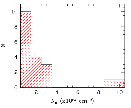
Figure 1: The column density distribution for all 19 sources in our sample.

Figure 2: The reflection fraction distribution ($f^{refl}=Flux[S0]/(Flux[Z]+Flux[S90]+Flux[S0]$ ) in the 20-40 keV band for all 19 sources in our sample

.

Figure 3: The coronal temperature distribution as estimated using the COMPTT model of Titarchuk (1994) (16 sources). The three sources in which kT is unconstrained have been excluded.

Table 2: MYTORUS Spectral fits

Name	$\rm N_{H},Z$	$\rm kT$	$\tau$	$\rm E_{C}$	$f^{refl}_{20-40keV}$	$\rm\chi^{2}/d.o.f.$	Ref.
(1)	(2)	(3)	(4)	(5)	(6)	(7)	(8)
NGC1068	$>10$	$67^{+97.0}_{-28.0}$	$0.68^{+0.08}_{-0.23}$	$>$145	0.84	890/755	a, i
Circinus	$9.0^{+1.00}_{-0.50}$	$38^{+9.5}_{-7.6}$	$0.61^{+0.10}_{-0.08}$	$43^{+5}_{-4}$	0.80	1872/1724	b
NGC6240	$1.3_{-0.22}^{+0.12}$	$60_{-20.6}^{+85.5}$	$1.7_{-0.73}^{+0.23}$	unconstr.	$<0.01$	456/496	c, i
NGC4945	$3.5_{-0.13}^{+0.20}$	$59_{-13.3}^{+19.7}$	$1.7_{-0.32}^{+0.34}$	$>$42	$0.02$	1786/1743	d, i
NGC424	$1.3_{-0.20}^{+0.25}$	$30_{-12.1}^{+20.9}$	2	$>$64	0.93	147/121	e, i
2MFGC2280	$1.6_{-0.45}^{+0.72}$	50	$1.3_{-1.3}^{+1.4}$	$<$238	0.03	66/59	i
NGC1194	$1.7_{-0.25}^{+0.24}$	$37_{-1.0}^{+4.7}$	$1.5_{-0.13}^{+0.30}$	unconstr.	$<0.01$	257/273	f
MCG+06-16-028	$1.5_{0.27}^{+0.42}$	$34_{-18.1}^{+20.0}$	$1.4^{+0.7}_{-1.3}$	$>23$	0.04	136/132	i
NGC3079	$3.2_{-0.43}^{+0.54}$	$31_{-8.1}^{+8.6}$	2	$56^{+354}_{-24}$	0.05	192/165	i
NGC3393	$2.1_{-0.28}^{+0.61}$	$69_{-60.9}^{+77.9}$	$1.05_{-1.05}^{+0.97}$	$>96$	$<0.01$	123/117	g, i
NGC4941	$1.2_{-0.39}^{+0.91}$	$47^{+216}_{-34}$	2	unconstr.	0.19	98/111
NGC5728	$1.3_{-0.08}^{+0.13}$	$81_{-30.2}^{+48.6}$	$1.5_{-0.41}^{+0.32}$	$121^{+11}_{-13}$	$<0.01$	444/436	i
ESO137-34	$2.9_{-0.54}^{+0.86}$	$26_{-11.8}^{+15.9}$	2	$>$203	0.12	175/147
NGC7212	$1.1_{-0.27}^{+0.48}$	$41^{+32.2}_{-22.6}$	2	$>56$	$<$0.01	147/117	i
NGC1229	$0.6_{-0.14}^{+0.26}$	$60^{+51.2}_{-22.5}$	2	unconstr.	$<0.01$	134/138	i
NGC6232	$0.8_{-0.30}^{+1.26}$	$42_{-29.5}^{+40.2}$	2	$>$500	$<0.01$	52/35	i
2MASXJ09235371	$1.0_{-0.18}^{+0.21}$	$60_{-27.9}^{+68.1}$	2	$35^{+6.1}_{-5.1}$	$<0.01$	266/209	i
NGC5643	$1.3^{+0.10}_{-0.10}$	50	2	$>$48	0.92	136/127	h,i
NGC7130	$2.3_{-0.31}^{+0.29}$	50	2	unconstr.	0.23	116/126	i

• (1) Source name (2) Average column density ($N_{H},Z=N_{H},S90=N_{H},S0$) in units of $\rm 10^{24}cm^{-2}$ (3) coronal temperature (keV); values with no error bar were unconstrained and have been fixed to a value of 50 keV. (4) optical depth; values with no error bars were unconstrained and have been fixed to a value of $\rm\tau=2$. (5) the high energy cut-off derived by Ricci et al. (2017) from Niel Gehrels Swift, XMM-Newton, Chandra joint fits. (6) unobscured reflected fraction in the 20-40 keV band. The unobscured reflection fraction is defined as $\rm Flux[S0]/(Flux[Z]+Flux[S90]+Flux[S0])$ (8) $\chi^{2}$ over degrees of freedom (9) Reference for previous NuSTAR   analyses: (a) Bauer et al. (2015); (b) Arévalo et al. (2014) ; (c) Puccetti et al. (2014); (d) Puccetti et al. (2016); (e) Baloković et al. (2014); (f) Masini et al. (2016) (g) Koss et al. (2015) (h) Annuar et al. (2015) (i) Marchesi et al. (2018).

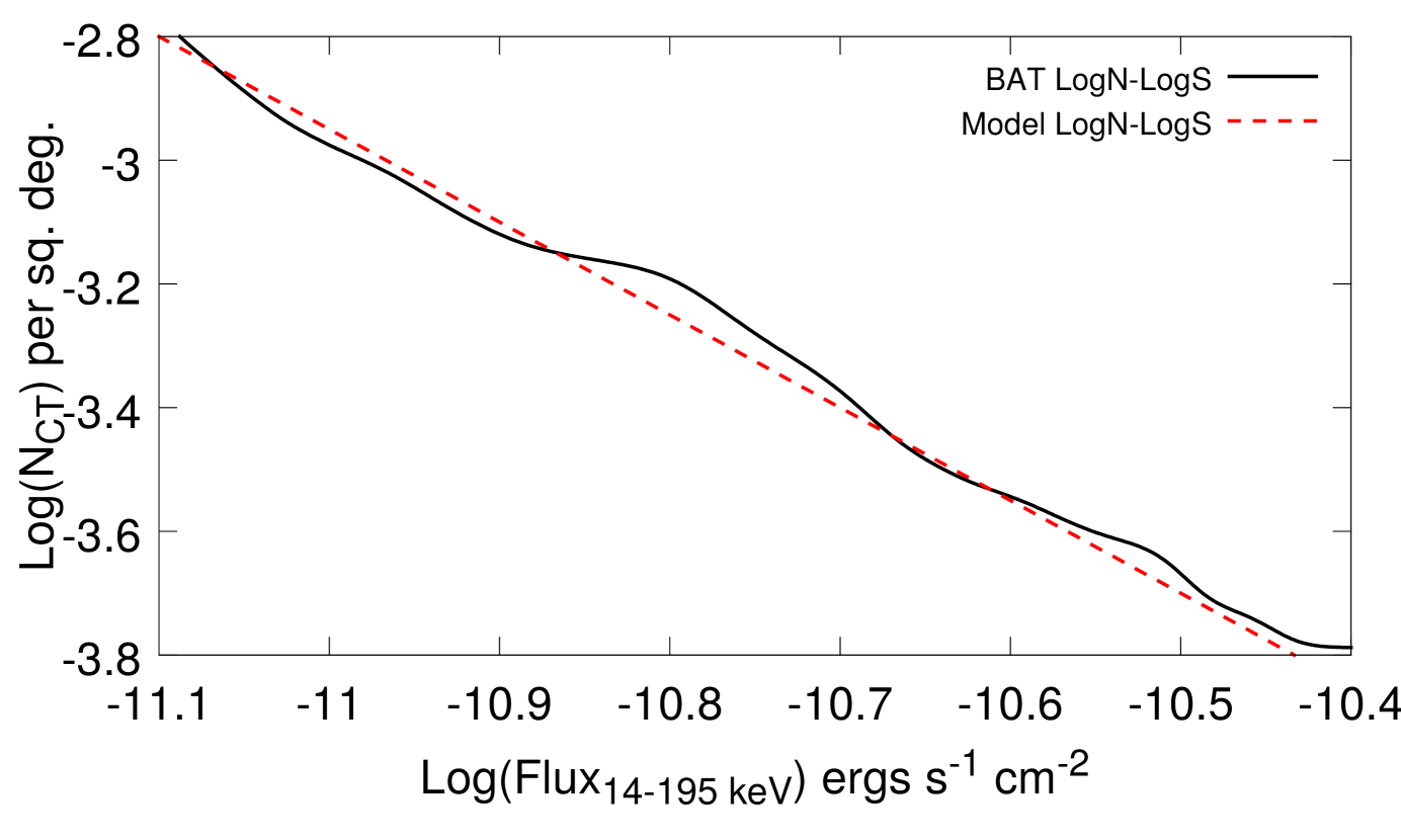
Figure 4: The number count distribution of the Compton-thick AGN derived from the Niel Gehrels SWIFT-BAT survey in Akylas et al. (2016) (black solid line). The red dashed line denotes the prediction of the X-ray population synthesis model of Akylas et al. (2012). Using the spectral parameters found in our spectral fits, we find that the Compton-thick AGN fraction should be 20% of the type-2 AGN population, in order to agree with the observed logN-logS.

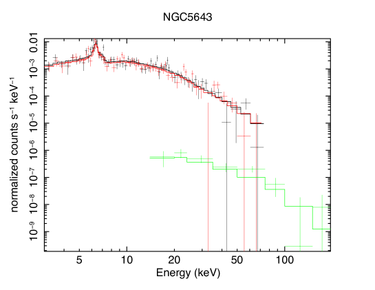
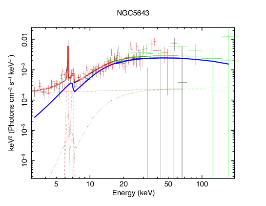
Figure 5: NGC5643: a characteristic spectrum of an AGN with a high reflection component. Upper panel: folded spectrum. Bottom panel: unfolded spectrum; the blue sold line denotes the unabsorbed component S0. The straight dotted line represents the soft power-law component while the other dotted line denotes the absorbed reflection component S90. In both panels the black and red colours denote the two FPM NuSTAR detectors while the green colour corresponds to the BAT detector.

4 Results

The spectral-fitting results are given in table LABEL:spectral-fits. In the following subsections we discuss separately our findings regarding the hydrogen column density, the high energy cut-off and the reflection fraction. Finally, we discuss the implications of our spectral modelling for the intrinsic number of Compton-thick AGN.

4.1 Absorbing column density

The distribution of the column densities is presented in Fig. 1. The column densities found by NuSTAR are in very good agreement with those previously found by Niel Gehrels Swift (Akylas et al., 2016). Only for one source (NGC7212), Akylas et al. (2016) find a much higher column density. The current NuSTAR results confirm the lower column density reported by Ricci et al. (2015). This difference is most probably because the Niel Gehrels Swift/XRT data have limited photon statistics while Ricci et al. (2015) have combined the BAT data with XMM-Newton spectra obtaining better quality photon statistics at energies below 10 keV. Recently, Marchesi et al. (2018) published a NuSTAR analysis of Compton-thick AGN from the Niel Gehrels SWIFT/BAT list of Ricci et al. (2015). Marchesi et al. (2018) find that a number of candidate Compton-thick AGN in Ricci et al. (2015) may present lower column densities. There are 15 common objects between our sample and that of Marchesi et al. (2018). According to these authors four objects appear to have column densities somewhat lower than $\rm 10^{24}cm^{-2}$. These are NGC1194, NGC6232, NGC1229 and 2MASSXJ09235371-3141305. According to our NuSTAR analysis, NGC1194 is above the Compton-thick threshold while NGC1229 and 2MASSXJ09235371-3141305 are consistent with being Compton-thick within the errors. In the case of NGC1229, although the source is unambiguously heavily obscured ($\rm N_{H}\approx 6^{+2.6}_{-1.4}\times 10^{23}cm^{-2}$ ) the column density derived lies well below the Compton-thick limit. For many other sources, e.g. NGC1068, Circinus, NGC424, NGC3079, NGC4945, NGC5643, NuSTAR spectral fits have been presented elsewhere (Bauer et al., 2015; Arévalo et al., 2014; Baloković et al., 2014; Puccetti et al., 2016; Koss et al., 2015; Puccetti et al., 2014; Annuar et al., 2015; Marchesi et al., 2018). In general, our results are consistent with the work cited above.

As it can be seen from Fig. 1, there is a clear tendency to detect mildly obscured Compton-thick AGN with column densities a few times $\rm 10^{24}cm^{-2}$. This has been first noticed by Burlon et al. (2011) who showed that the BAT instrument is unbiased only up to column densities of only $\rm 2\times 10^{24}cm^{-2}$. We observe only two heavily Compton-thick source with a column density around $\rm 10^{25}cm^{-2}$. Owing to their diminished X-ray emission, these heavily obscured sources can be detected only if they are relatively nearby. A similar effect is observed in INTEGRAL observations of Compton-thick AGN (Malizia et al., 2009). Although the number of Compton-thick AGN is relatively limited in the current sample, Akylas et al. (2016) using a much larger sample noticed that the column density distribution is fully consistent with a flat Compton-thick column density distribution between $10^{24}$ and $10^{26}$ $\rm cm^{-2}$.

4.2 High energy cut-off

In column (3) of table LABEL:spectral-fits we give the derived coronal temperature. The cut-off energy corresponds to $\sim 3kT$ (Titarchuk, 1994). For three objects the coronal temperature could not be constrained (2MFGC2280, NGC5643, NGC7130). The mean energy of the coronal temperature of the remaining 16 sources is $\rm kT\approx 50$ keV corresponding to a high energy cut-off of about $\rm E_{C}\sim 150$ keV. The distribution of the coronal temperature is given in Fig. 3. In the case of the three sources above where the coronal temperature could not be well constrained, we fixed the temperature at 50 keV in order to estimate the reflected emission.

It is interesting to compare the estimated cut-off with other high energy spectral studies of Compton-thick AGN. Dadina (2007) estimated the cut-off energy in a number of nearby AGN using data from the BeppoSAX mission which observes in the 2-100 keV range. There are eight sources in common between our sample and that of Dadina (2007). Owing to the limited photon statistics at high energies, Dadina (2007) were able to constrain the high-energy cut-off in only two of these sources; NGC1068, with $\rm E_{C}>116$ keV and NGC4945 with $\rm E_{C}=122^{+41}_{-26}$ keV. These values are entirely consistent with our combined NuSTAR and BAT analysis. Ricci et al. (2017) derived the cut-off energy of the Compton-thick AGN in his sample using a combination of XMM-Newton , Chandra, and Niel Gehrels Swift spectra (both XRT and BAT). For comparison with the present work, the cut-off energies, $\rm E_{C}\sim 3kT$, derived by Ricci et al. (2017), are given in column (5) of table LABEL:spectral-fits. In many cases, there is reasonable agreement between the two analyses. However, there are at least four cases where the results are clearly at odds. These are Circinus, ESO137-34, NGC6232 and 2MASXJ09235371. This discrepancy could be partly attributed to the different spectral models used that is power-law model with an exponential cut-off versus the comptonization models. Ricci et al. (2017) have determined the average cut-off energy for their Compton-thick sources. When they exclude the lower and upper limits, they find a very low high energy cut-off for their Compton-thick AGN ($\rm E_{C}\approx 43\pm 15$ keV). Taking lower and upper limits into account by means of the Kaplan-Meier estimator, they estimate a much higher value for the cut-off $\rm E_{C}\sim 450\pm 64$ keV. We find a mean high energy cut-off of $\rm E_{C}\sim 3kT\approx 150$ keV, excluding the three sources above where the cut-off energy could not be constrained. It is also interesting to compare with the work of Dadina (2007) who derived the average X-ray spectrum of 42 type-2 AGN using BeppoSAX data. They find a cut-off energy of $\rm E_{C}=376\pm 42$ keV. This is significantly higher than the cut-off energy of our Compton-thick sources.

Our results are not significantly affected by the choice of $\tau=2.0$ in the cases where the photon statistics is limited. For example, in the case of NGC3079 if we choose $\tau=1.5$, the resulting temperature becomes $\rm kT=39\pm 19$ keV. For this temperature of the corresponding photon index would be $\Gamma\approx 2.0$.

4.3 Reflection component

The fraction of the reflected emission in the 20-40 keV band plays an important role in the prediction of the intrinsic Compton-thick AGN fraction, in the sense that as the reflected emission becomes higher, the number of Compton-thick AGN required is reduced. This is because the higher the reflection the easier is to detect Compton-thick AGN in the BAT band and hence the number of ’missing’ Compton-thick AGN is relatively small. The reflection fraction is given in column (6) of table 2. This is defined as the ratio of the unabsorbed reflection component S0 versus the total flux i.e. the sum of the line of sight component Z and the two scattered components S0 and S90. Four sources appear to be reflection dominated as the reflection radiation fraction is near unity. These are NGC1068, Circinus, NGC424 and NGC5643. A typical spectrum of a source with a strong reflection component (NGC5643) is shown in Fig. 5. There is not a clear correlation between the strength of the reflection component and the column density in these sources. For example, NGC424 and NGC5643 have ’moderate’ Compton-thick column densities 1.3 $\rm\times 10^{24}cm^{-2}$. The vast majority of the sources have moderate strength reflection components below 0.23. There are eight sources where the best-fit reflection component is negligible i.e. well below 0.01. The distribution of the reflection fraction is given in Fig. 2. The mean reflection fraction is 0.22. In analogy to the commonly used PEXRAV model (Magdziarz & Zdziarski, 1995), which estimates the reflection to an infinite slab, we find that a fraction of 0.22 corresponds to a reflection strength R$\approx$1. This is equivalent to a reflection fraction of $\sim$3% in the 2-10 keV band.

4.4 The intrinsic fraction of Compton-thick AGN

In this section we estimate the intrinsic number of Compton-thick AGN in the Universe using the population synthesis models developed by Akylas et al. (2012). The X-ray background synthesis models have been primarily being devised in order to predict the number of Compton-thick AGN based on their contribution to the X-ray background spectrum and in particular at its energy peak around 20-30 keV. The X-ray background synthesis models predict the number of AGN and their contribution to the X-ray background spectrum at any redshift, luminosity and column density. The necessary ingredients are the AGN luminosity function and the typical AGN spectrum. Treister et al. (2009) first pointed out that uncertainties on the measurements of the X-ray background are substantially large to hamper an accurate prediction of the number of Compton-thick AGN. Instead they propose that the INTEGRAL or BAT number counts of Compton-thick AGN place tighter constraints. In this manner, the X-ray background synthesis models could be used to extrapolate the observed number counts to the intrinsic population number counts. In a similar approach, Burlon et al. (2011) use the observed Compton-thick AGN number counts and predict the intrinsic Compton-thick AGN counts by assuming a relation between the observed and the intrinsic Compton-thick flux. This conversion sensitively depends on the typical Compton-thick AGN spectrum. Using a simple spectrum and by deriving the intrinsic $\rm N_{H}$ distribution, Burlon et al. (2011) derive an intrinsic Compton-thick AGN contribution of $\sim$20%.

Here, we fold the full observed spectral distribution as described by the parameters $\rm N_{H}$, kT and the reflection fraction (see Fig.1, Fig.2 and Fig.3) in our X-ray population synthesis models. Then, the remaining unknown parameter is the intrinsic fraction of Compton-thick AGN. We find that in order to match the observed Compton-thick AGN counts in the BAT 14-195 keV band with our models, we need an intrinsic fraction of $\sim$20% relative to the type-II AGN population ($\rm N_{H}>10^{22}cm^{-2}$), see Fig. 4. This corresponds to a Compton-thick fraction of 15% relative to the total AGN population. The statistical error on this figure is 3%. This is derived from the number of Compton-thick AGN ($53\pm 7$) used to derive the logN-logS. The uncertainties on the spectral parameters estimated above have not been taken into account in this error estimate.

Recently, Masini et al. (2018) estimated the Compton-think fraction of Compton-thick sources, using NuSTAR observations in the UKIDSS Ultra deep field. They find an observed Compton-thick fraction of $8.4\pm 2\%$ in the 8-24 keV band at a flux of $2.7\times 10^{-14}$ $\rm erg\leavevmode\nobreak\ cm^{-2}\leavevmode\nobreak\ s^{-1}$. Making corrections for their non-detected XMM-Newton sources this fraction becomes $11.5\pm 2.0$. This is in agreement with the 1$\sigma$ upper limit of our model predictions which is $\approx 10\%$ at this flux.

5 Summary and Conclusions

Direct spectroscopic observations of AGN in the local Universe, using Niel Gehrels Swift/BAT samples, find a fraction of Compton-thick AGN of about 7% (Burlon et al., 2011; Ricci et al., 2015; Akylas et al., 2016; Marchesi et al., 2018). This figure can be extrapolated to the intrinsic number of Compton-thick AGN by assuming a spectral model for the Compton-thick AGN spectrum (e.g. Burlon et al., 2011). The spectral parameters of interest are the photon index, the strength of the reflection component, the column density distribution, and the primary emission cut-off energy. The reflection of material on cold matter surrounding the nucleus results in the flattening of the spectrum around 20-30 keV. Therefore the higher the reflection the easier is to detect Compton-thick AGN in the 14-195 keV band and hence the lower the number of missing Compton-thick AGN (the lower the intrinsic fraction). The high energy cut-off works in the opposite way. The lower the value of the cut-off energy, the higher the intrinsic number of Compton-thick AGN as these would not be easily detected in the BAT band. For example, if the high energy cut-off were $\approx$50keV (see e.g. Ricci et al., 2017), the fraction of Compton-thick AGN fraction would increase to about 50%. Note that in contrary, cut-offs higher than 150 keV would not significantly affect our results.

Aiming to constrain the intrinsic fraction of Compton-thick AGN in the local Universe, we explore the spectrum of a large number Compton-thick AGN. We analyse the combined NuSTAR/BAT spectra of 19 candidate Compton-thick AGN (at the 70% confidence level) in the sample ofAkylas et al. (2016). We model the spectra using the MYTORUS models of Yaqoob (2012) which take into account absorption and reflection from Compton-thick material. The primary X-ray emission from a hot corona is modelled with a physically motivated model (Titarchuk, 1994). Our results can be briefly summarised as follows.

• We derive absorbing column densities which are consistent with those derived by the previous Niel Gehrels Swift/BAT analyses by Ricci et al. (2015) and Akylas et al. (2016) .

• We estimate that the coronal temperatures lie between 25 and 80 keV corresponding to high energy cut-offs roughly between 75 and 240 keV. The mean cut-off energy is 150 keV.

• We find that a large fraction of our AGN lack a significant reflection component in the 20-40 keV band. The average reflection fraction is $\sim$0.22 .

• The resulting spectral parameters are used to place constraints on the intrinsic Compton-thick AGN fraction. Using the above spectral results in combination with our synthesis models, we extrapolate the observed fraction of Compton-thick AGN to the intrinsic fraction. We find that the Compton-thick AGN fraction is $20\pm 3$% of the type-II AGN population.