Digging the population of compact binary mergers out of the noise

Abstract

Coalescing compact binaries emitting gravitational wave (GW) signals, as recently detected by the Advanced LIGO-Virgo network, constitute a population over the multi-dimensional space of component masses and spins, redshift, and other parameters. Characterizing this population is a major goal of GW observations and may be approached via parametric models. We demonstrate hierarchical inference for such models with a method that accounts for uncertainties in each binary merger’s individual parameters, for mass-dependent selection effects, and also for the presence of a second population of candidate events caused by detector noise. Thus, the method is robust to potential biases from a contaminated sample and allows us to extract information from events that have a relatively small probability of astrophysical origin.

I Introduction

Since the first detection of gravitational waves in 2015 Abbott et al. (2016a), the Advanced LIGO and Advanced Virgo detectors have observed the coalescence of multiple compact binary systems, and have begun to reveal the population of coalescing compact objects Abbott et al. (2016b). This population is enabling studies in fields from probing alternative theories of gravity to constraining models of stellar evolution. These tend to be interested either in individual, preferably loud, signals, or in the population of sources as a whole. The latter type of population analysis tries to estimate the parameters governing the distribution of sources in the universe, their masses and spins, and the value of the astrophysical merger rate Abbott et al. (2016c) are of particular interest. As the sensitivity of detectors improves over the coming years, the detected number of sources is expected to grow at an accelerated pace, rapidly increasing the amount of information available for population studies Abbott et al. (2018).

When undertaking population analyses, one has to consider that real detectors may produce noise transients which cannot in all cases be distinguished from astrophysical GW sources. To avoid population inferences being biased by noise events one might consider only events with a much higher probability to be of astrophysical origin than to be caused by noise artefacts. In templated searches for compact binaries, the relative probability of astrophysical vs. noise origin for a candidate event is a function of a detection statistic calculated for each event by a search analysis pipeline (see e.g. Abbott et al. (2016d); Usman et al. (2016); Cannon et al. (2012, 2015); Messick et al. (2017); Nitz et al. (2017)). Typically a candidate event is generated as a local maximum in matched filter signal-to-noise ratio (SNR) above a search threshold; the detection statistic value then incorporates the matched filter SNR, as well as other goodness-of-fit tests to reject non-Gaussian instrumental noise transients Allen (2005); Nitz (2018).

At low SNR, the population of events is dominated by the noise ‘background’, whereas at high SNR (or in general for events assigned high statistic values) the astrophysical ‘foreground’ dominates. To limit possible pollution of the sample used for population inference, one may place a minimum threshold on the detection statistic; any event above threshold is then assumed to be astrophysical, whereas all other events are discarded as potential noise transients. Note that the choice of threshold value requires an empirical estimate of the rate and distribution of background events Capano et al. (2017), since the rate, strength and morphologies of detector noise artefacts are not known a priori Abbott et al. (2016e).

A simple strategy of thresholding is sub-optimal for two reasons. First, discarding events below the threshold will almost certainly discard information from some number of quiet but still identifiable signals; second, there is still a finite chance that the resulting ‘signal’ set is nevertheless contaminated by noise, leading to potentially biased inferences. The choice of SNR threshold requires a trade-off between these two considerations and depends on the intended use. One also has to take into consideration any bias in the observed population produced by the effect of source parameters on the loudness of a signal, and thus its chance of exceeding a SNR threshold Fairhurst and Brady (2008); we expect potentially major observation selection effects for binary mass(es) Tiwari (2017) and component spins Ng et al. (2018).

Here, we propose a method which alleviates the issues associated with simple thresholding by applying a hierarchical mixture model under which each event is considered to originate from either a foreground or a background (noise) population. For each event, the probability of either case naturally defines a weight for its contribution to inferences on population parameters.

This method combines the processes of estimating the expected number of events in either class Farr et al. (2015) (the number of foreground events being a proxy for the astrophysical merger rate density) and estimating parameters of the underlying populations, which have previously been performed separately. It avoids being biased through the inclusion of background events, while being able to make use of events with a non-negligible probability of noise origin, which would be discarded by thresholding. In theory this method allows the SNR threshold to be reduced to an arbitrarily low value, though in practice we are still limited by the computational resources required to extract the source parameters from each event under consideration.

Our method is applicable to any hierarchical model of a source population, examples of which have been explored in the literature. This includes analyses which combine information from multiple events to infer a parameter common to all, such as deviations from general relativity Li et al. (2012) or a parameterised neutron star equation of state Del Pozzo et al. (2013). The use of a mixture model with astrophysical and noise populations is particularly useful when the model of interest has a strong effect on the detectability of sources, i.e. the detected events are unrepresentative of the underlying population. A good example is the mass distribution of sources, which we consider below.

Messenger and Veitch (2013) considered the problem of selection effects in mass distribution inference by dividing the observing time into discrete chunks, which each contain zero or one sources, and computing population likelihoods while accounting for false alarms and false dismissals from an idealised noise distribution. Farr et al. (2015) derived an equivalent formalism for rate inference that allows a population shape function to be estimated alongside. Our derivation in Section II follows similar lines.

The selection function for masses was important in estimating the astrophysical event rates in the first Advanced LIGO observing run (O1), which inferred rates using a mixture model, for fixed choices of population shape (i.e. mass distribution) Abbott et al. (2016c, f). A separate analysis also estimated the slope of a power law model of the mass distribution function considering the detected events, described in Abbott et al. (2016b) (and updated in Abbott et al. (2017)).

The selection function in the form of a sensitivity-weighted measure of the space-time volume $VT$ is also important when considering searches which do not make a clear detection. There, the loudest background event, or a nominal detection threshold, is used to set an upper limit on the astrophysical rate of a fiducial source population, for example limits on the rate of mergers of binary neutron stars and neutron star–black hole binaries in O1 Abbott et al. (2016g). The sensitive-volume approach has been in use since the initial detector era Biswas et al. (2009); Abadie, J. et al. (2011), and continues to be refined to incorporate mass- and spin-dependent selection effects O’Shaughnessy et al. (2010); Dominik et al. (2015); Ng et al. (2018) and cosmological effects, as well as to improve the accuracy of measurement Tiwari (2017).

As the number of detections increases, determination of the population of coalescing compact binaries is expected to provide insight into the astrophysics of black hole and neutron star binary formation, as reviewed in Kalogera et al. (2007); Abbott et al. (2016h); Mandel and Farmer (2018)). Population synthesis models can describe the masses and spins of coalescing compact binaries under a variety of formation scenarios (see e.g. Belczynski et al. (2016, 2017, 2016); Spera et al. (2015)). Comparison of these predictions to the observed distribution can be used to constrain the uncertainties in parametrised models of source populations Barrett et al. (2017); Zevin et al. (2017). This has motivated the development of methods to determine the mass-dependent coalescence rate in the absence of false alarms, using both specific parameterised models Wysocki et al. (2018a, b); Talbot and Thrane (2018); Taylor and Gerosa (2018) and non-parametric methods Mandel et al. (2017). The alignment of black hole spins is expected to be a key distinguishing feature between binaries formed in the field or through dynamical interactions (see e.g. O’Shaughnessy et al. (2017); Mandel and O’Shaughnessy (2010); Gerosa et al. (2013); Stevenson et al. (2015); Farr et al. (2017); Stevenson et al. (2017); Gerosa and Berti (2017); Fishbach et al. (2017); Talbot and Thrane (2017)), which also requires an understanding of the spin selection function O’Shaughnessy et al. (2010); Dominik et al. (2015); Ng et al. (2018). The work presented here is complementary to these studies, as it aims to incorporate an astrophysical distribution model as part of a mixture with a noise component. As the observed population is limited by the sensitivity of Advanced ground-based detectors, the population of candidate sources at the greatest distances (lowest detection significance) will be contaminated with background events. We expect our method, using information from such sources, to improve both the precision and accuracy of merger rate and population parameter estimates; though as we will see, the degree of improvement depends on how easily the foreground and background populations can be separated by existing analyses.

We start by defining our notation and deriving the general form of the model in section II. Section III describes its application to a toy model of mass distribution inference in the presence of noise, and shows its application to a range of simple analytic population models. In section V we consider a more realistic simulated data set derived from an engineering run prior to the start of Advanced LIGO observations in 2015. We conclude in section VI.

II Derivation of the generic model

We consider a mixture of two populations, the astrophysical ‘foreground’ and terrestrial noise ‘background’: quantities defined analogously for both populations will be distinguished by the subscripts $\mathrm{F}$ or $\mathrm{B}$ respectively. Quantities without subscript will then refer to the total population which is the union of foreground and background.

The model is also hierarchical: each event, if assumed astrophysical, has a set of intrinsic properties such as component masses and spins, which we collectively denote $\gamma$. The distribution of these properties over each population is assumed to have a form described by a set of hyper-parameters. We do not have access to the ‘true’ values of properties for each event, only to a set of samples from a (typically Bayesian) estimate based on data around the event. These samples are derived under the assumption that the event is astrophysical, thus events that are in fact background will also be assigned parameter estimates.

We then define the core quantities used in the following derivation as

• $\rho_{i}$, $\{\rho$} : ranking statistic for one, resp. for all events in a given data set.

• $N_{\mathrm{obs}}$, $N_{\mathrm{F,obs}}$, $N_{\mathrm{B,obs}}$ : observed number of events above a threshold $\rho_{i}>{\rho_{\mathrm{thr}}}$

• $N_{\mathrm{exp}}$, $N_{\mathrm{F,exp}}$, $N_{\mathrm{B,exp}}$ : expected number of events with $\rho_{i}>{\rho_{\mathrm{thr}}}$, when modelling these as a Poisson process

• $\theta_{\mathrm{F}}$, $\theta_{\mathrm{B}}$ : hyper-parameters which describe the population distributions

• $\eta_{i}$, $\{\eta$} : flag indicating whether any given event, resp. all events, belong(s) to the astrophysical ($\eta=F$) or to the noise population ($\eta=B$)

• $\vec{\gamma}_{i}$, $\{\vec{\gamma}\}$ : vector of samples representing the parameter estimates (masses, spins, etc.) of one, resp. all events, under the assumption that events are astrophysical.

We wish to infer the joint posterior probability distribution of rates and population parameters for the two populations, given some events for which $\{\rho\}$ and $\{\vec{\gamma}\}$ have been determined by the search and parameter estimation stages of data analysis:

$$p(N_{\mathrm{F,exp}},N_{\mathrm{B,exp}},\theta_{\mathrm{F}},\theta_{\mathrm{B}}|\{\rho\},\{\vec{\gamma}\},{N_{\mathrm{obs}}}).$$ (1)

Using Bayes’ theorem we can express the posterior distribution (1) in terms of prior and likelihood functions,

$$p(N_{\mathrm{F,exp}},N_{\mathrm{B,exp}},\theta_{\mathrm{F}},\theta_{\mathrm{B}}|\{\rho\},\{\vec{\gamma}\},{N_{\mathrm{obs}}}) =\frac{p(\{\rho\},\{\vec{\gamma}\},{N_{\mathrm{obs}}}|N_{\mathrm{F,exp}},N_{\mathrm{B,exp}},\theta_{\mathrm{F}},\theta_{\mathrm{B}})p(N_{\mathrm{F,exp}},N_{\mathrm{B,exp}},\theta_{\mathrm{F}},\theta_{\mathrm{B}})}{p(\{\rho\},\{\vec{\gamma}\},{N_{\mathrm{obs}}})}$$ (2)

We drop the normalisation constant $p(\{\rho\},\{\vec{\gamma}\},{N_{\mathrm{obs}}})$ and factor out the likelihood for ${N_{\mathrm{obs}}}$ as being independent of the population shape parameters,

$$p(\{\rho\},\{\vec{\gamma}\},{N_{\mathrm{obs}}}|N_{\mathrm{F,exp}},N_{\mathrm{B,exp}},\theta_{\mathrm{F}},\theta_{\mathrm{B}}) =p({N_{\mathrm{obs}}}|N_{\mathrm{F,exp}},N_{\mathrm{B,exp}})p(\{\rho\},\{\vec{\gamma}\}|N_{\mathrm{F,exp}},N_{\mathrm{B,exp}},\theta_{\mathrm{F}},\theta_{\mathrm{B}})$$

$$=\frac{N_{\mathrm{exp}}^{N_{\mathrm{obs}}}e^{-N_{\mathrm{exp}}}}{{N_{\mathrm{obs}}}!}p(\{\rho\},\{\vec{\gamma}\}|N_{\mathrm{F,exp}},N_{\mathrm{B,exp}},\theta_{\mathrm{F}},\theta_{\mathrm{B}}),$$ (3)

where we use a Poisson likelihood for ${N_{\mathrm{obs}}}$ with a total expected number of events $N_{\mathrm{exp}}=N_{\mathrm{F,exp}}+N_{\mathrm{B,exp}}$. The second term, $p(\{\rho\},\{\vec{\gamma}\}|N_{\mathrm{F,exp}},N_{\mathrm{B,exp}},\theta_{\mathrm{F}},\theta_{\mathrm{B}})$, is the likelihood for the observed SNRs and parameter estimates, for the mixture model. We assume each event is conditionally independent given the population parameters, and so the joint likelihood is just the product of the likelihood for each one,

$$p(\{\rho\},\{\vec{\gamma}\}|N_{\mathrm{F,exp}},N_{\mathrm{B,exp}},\theta_{\mathrm{F}},\theta_{\mathrm{B}})=\prod_{i}p(\rho_{i},\vec{\gamma}_{i}|N_{\mathrm{F,exp}},N_{\mathrm{B,exp}},\theta_{\mathrm{F}},\theta_{\mathrm{B}}).$$ (4)

Now, we can split each of these into terms for the astrophysical and noise sub-models by introducing an indicator variable $\eta_{i}\in(F,B)$, whose probability will depend on the rate parameters $N_{\mathrm{F,exp}}$ and $N_{\mathrm{B,exp}}$,

$$p(\rho_{i},\vec{\gamma}_{i}|N_{\mathrm{F,exp}},N_{\mathrm{B,exp}},\theta_{\mathrm{F}},\theta_{\mathrm{B}}) =p(\rho_{i},\vec{\gamma}_{i}|\theta_{\mathrm{F}},\eta_{i}\!=\!\mathrm{F})p(\eta_{i}\!=\!\mathrm{F}|N_{\mathrm{F,exp}},N_{\mathrm{B,exp}})$$

$$\qquad+p(\rho_{i},\vec{\gamma}_{i}|\theta_{\mathrm{B}},\eta_{i}\!=\!\mathrm{B})p(\eta_{i}\!=\!\mathrm{B}|N_{\mathrm{F,exp}},N_{\mathrm{B,exp}})$$

$$=p(\rho_{i},\vec{\gamma}_{i}|\theta_{\mathrm{F}},\eta_{i}\!=\!\mathrm{F})\frac{N_{\mathrm{F,exp}}}{N_{\mathrm{exp}}}+p(\rho_{i},\vec{\gamma}_{i}|\theta_{\mathrm{B}},\eta_{i}\!=\!\mathrm{B})\frac{N_{\mathrm{B,exp}}}{N_{\mathrm{exp}}},$$ (5)

where the probability of each class is just the expected fraction of the total number. Since this is a sum of probability densities, special care must be taken to ensure all terms are properly normalised, such that

$$\int^{\infty}_{{\rho_{\mathrm{thr}}}}\mathrm{d}{\rho}\>\int\mathrm{d}{\gamma}\>p(\rho,\gamma|\theta_{\eta},\eta_{i})=1,$$ (6)

for $\eta=\mathrm{F}$ and $\eta=\mathrm{B}$, where ${\rho_{\mathrm{thr}}}$ is a minimum SNR value for which events are considered, either as a result of the event generation method or as a choice to limit computational costs. Neglecting this normalization would introduce an artificial preference for one component over the other. An extension to further sub-populations is simply achieved by including additional classes with their own rate and shape parameters.

Recombining the pieces, we can write the desired posterior in Eq. (1) as

$$p(N_{\mathrm{F,exp}},N_{\mathrm{B,exp}},\theta_{\mathrm{F}},\theta_{\mathrm{B}}|\{\rho\},\{\vec{\gamma}\},{N_{\mathrm{obs}}})\propto\\ p(N_{\mathrm{F,exp}},N_{\mathrm{B,exp}},\theta_{\mathrm{F}},\theta_{\mathrm{B}})e^{-N_{\mathrm{exp}}}\prod_{i}\big{[}\,p(\rho_{i},\vec{\gamma}_{i}|\theta_{\mathrm{F}},\eta_{i}\!=\!\mathrm{F})N_{\mathrm{F,exp}}+p(\rho_{i},\vec{\gamma}_{i}|\theta_{\mathrm{B}},\eta_{i}\!=\!\mathrm{B})N_{\mathrm{B,exp}}\,\big{]}.$$ (7)

This expression is similar to Eq.(21) from Farr et al. (2015) with an explicitly added dependence on source parameter estimates. This implies that our formalism reduces to the Farr et al. (2015) result as used by LVC to estimate binary black hole merger rates Abbott et al. (2016b, c), if the event distribution over mass or similar parameters is not free to vary.

The dependence on event parameters arises through the use of samples $\vec{\gamma}_{i}$, $i=1\ldots n$, drawn from the likelihood function of the data $d$ for a given point in parameter space $p(d|\gamma)$. These allow us evaluate the population likelihood function via marginalisation over the unknown true parameters, using the $n$ samples to perform a Monte Carlo integral as in Mandel (2010),

$$p(d|\theta_{\mathrm{F}}) =\int p(d|\gamma)p(\gamma|\theta_{\mathrm{F}})\mathrm{d}{\gamma}\>$$

$$=\left<p(\vec{\gamma}_{i}|\theta_{\mathrm{F}})\right>_{p(d|\vec{\gamma}_{i})}$$

$$=n^{-1}\sum_{j}p(\gamma_{j}|\theta_{\mathrm{F}}).$$ (8)

Samples from the likelihood therefore serve as a useful intermediate representation of the raw interferometer data $d$.

To obtain a quantity directly relevant for an astrophysical interpretation, the expected number can be transformed into the local merger rate $R$ using the observing time $T$ and the sensitive volume $V(\gamma)$:

$$R=\frac{N_{\mathrm{F,exp}}}{T\int\mathrm{d}{\gamma}\>V(\gamma)p(\gamma|\theta_{\mathrm{F}})},$$ (9)

where the integral marginalises over the space of source parameters $\gamma$. In practice $V(\gamma)$ is estimated for a particular data-set by a Monte Carlo campaign, adding (‘injecting’) a large number of simulated signals to the data and counting the resulting number of events above threshold.

An additional quantity which is not directly used in the derivation of our model, but is important for an astrophysical interpretation, is the probability of any given event originating from to the astrophysical foreground $p_{\mathrm{astro}}$:

$$p(\eta_{i}\!=\!\mathrm{F},N_{\mathrm{F,exp}},N_{\mathrm{B,exp}},\theta_{\mathrm{F}},\theta_{\mathrm{B}}|\rho_{i},\vec{\gamma}_{i})=\frac{p(\rho_{i},\vec{\gamma}_{i}|\theta_{\mathrm{F}},\eta_{i}\!=\!\mathrm{F})N_{\mathrm{F,exp}}\times p(N_{\mathrm{F,exp}},N_{\mathrm{B,exp}},\theta_{\mathrm{F}},\theta_{\mathrm{B}})}{p(\rho_{i},\vec{\gamma}_{i}|\theta_{\mathrm{F}},\eta_{i}\!=\!\mathrm{F})N_{\mathrm{F,exp}}+p(\rho_{i},\vec{\gamma}_{i}|\theta_{\mathrm{B}},\eta_{i}\!=\!\mathrm{B})N_{\mathrm{B,exp}}},$$ (10)

$$p_{\mathrm{astro},i}=\int_{0}^{\infty}\mathrm{d}{N_{\mathrm{F,exp}}}\>\int_{0}^{\infty}\mathrm{d}{N_{\mathrm{B,exp}}}\>\int\mathrm{d}{\theta_{\mathrm{F}}}\>\int\mathrm{d}{\theta_{\mathrm{B}}}\>p(\eta_{i}\!=\!\mathrm{F},N_{\mathrm{F,exp}},N_{\mathrm{B,exp}},\theta_{\mathrm{F}},\theta_{\mathrm{B}}|\rho_{i},\vec{\gamma}_{i}),$$ (11)

where we marginalised over the population parameters.

III Toy model

We construct a simple toy model of the universe to test our inference framework in various ways. The toy model allows us to generate a large number of realisations from the same underlying parameters, and to be certain that we use the correct model when analysing these realisations. For simplicity we consider a static, flat, and finite universe. Events are characterised completely by the distance $r$ to the source and a single mass parameter $m$, which takes the place of the $\gamma$ used in the previously derived expressions. This mass parameter can be thought of as similar to the chirp mass. Additional effects such as inclination, spins, mass ratio, or antenna patterns are ignored.

For our detection statistic $\rho$ we simply use (a simplified proxy for) the SNR, whose expected value ${\rho_{\mathrm{true}}}$ is determined by $r$ and $m$ as

$${\rho_{\mathrm{true}}}=K\frac{m}{r}.$$ (12)

where $K$ is an arbitrary constant which quantifies the detector sensitivity. We also model the uncertainty in the estimation of the mass parameter as

$$\sigma_{\mathrm{PE}}\propto\frac{m}{\rho}$$ (13)

which is a simplification of the relation given in Cutler and Flanagan (1994).

To apply the generic form found in Eq. (7) to a specific problem, we need to evaluate the terms $p(\rho_{i},\vec{m}_{i}|\theta_{\mathrm{F}},\eta_{i}\!=\!\mathrm{F})$ and $p(\rho_{i},\vec{m}_{i}|\theta_{\mathrm{B}},\eta_{i}\!=\!\mathrm{B})$. This involves finding a functional form for the selection effects. For sources distributed uniformly in our static universe we can derive the needed expression directly by manipulating the joint distribution of masses and observed (detection) SNRs ${\rho_{\mathrm{obs}}}$. We use the SNR relation defined above in Eq. (12), which defines a mass dependent lower cut-off ${\rho_{\mathrm{cutoff}}}(m)=K\ m\ r_{U}^{-1}$ to the $\rho_{\mathrm{true}}$ possible in our toy universe. Additionally we use the fact that the euclidean distances $r=|\vec{x}|$ of sources distributed uniformly in volume follow a $r^{2}$-distribution. Therefore

$$p({\rho_{\mathrm{obs}}},m) =\int_{V_{U}}\mathrm{d}{\vec{x}}\>p({\rho_{\mathrm{obs}}},m|\vec{x})p(\vec{x})$$

$$=\frac{1}{V_{U}}\int_{0}^{r_{U}}\mathrm{d}{r}\>4\pi r^{2}p({\rho_{\mathrm{obs}}},m|r)$$

$$=\frac{1}{V_{U}}\int_{0}^{r_{U}}\mathrm{d}{r}\>\int_{{\rho_{\mathrm{cutoff}}}(m)}^{\infty}\mathrm{d}{{\rho_{\mathrm{true}}}}\>4\pi r^{2}p({\rho_{\mathrm{obs}}}|{\rho_{\mathrm{true}}})p({\rho_{\mathrm{true}}}|m,r)p(m)$$

$$=\frac{4\pi p(m)}{V_{U}}\int_{{\rho_{\mathrm{cutoff}}}(m)}^{\infty}\mathrm{d}{\hat{\rho}}\>\int_{{\rho_{\mathrm{cutoff}}}(m)}^{\infty}\mathrm{d}{{\rho_{\mathrm{true}}}}\>p({\rho_{\mathrm{obs}}}|{\rho_{\mathrm{true}}})\frac{(Km)^{3}}{\hat{\rho}^{4}}\delta(\hat{\rho}-{\rho_{\mathrm{true}}})$$

$$=\frac{4\pi K^{3}m^{3}p(m)}{V_{U}}\int_{{\rho_{\mathrm{cutoff}}}(m)}^{\infty}\mathrm{d}{{\rho_{\mathrm{true}}}}\>\rho_{\mathrm{true}}^{-4}\>p({\rho_{\mathrm{obs}}}|{\rho_{\mathrm{true}}})$$

$$\propto m^{3}p(m)\int_{{\rho_{\mathrm{cutoff}}}(m)}^{\infty}\mathrm{d}{{\rho_{\mathrm{true}}}}\>\rho_{\mathrm{true}}^{-4}\>p({\rho_{\mathrm{obs}}}|{\rho_{\mathrm{true}}}),$$ (14)

where $r_{U}$ and $V_{U}$ are the radius and volume of our universe, respectively, and ${\rho_{\mathrm{cutoff}}}(m)=\frac{Km}{r_{U}}$ is the lower SNR cut-off defined by a source of mass $m$ being placed at the maximum allowed distance $r_{U}$. Thus, the SNR distribution for astrophysical sources is $p(\rho)\propto\rho^{-4}$, and we expect the observed mass distribution to be biased by a factor of $m^{3}$. The mass and SNR components of Eq. (14) are generally connected via the mass dependent SNR cut-off. The term $p({\rho_{\mathrm{obs}}}|{\rho_{\mathrm{true}}})$ accounts for the shift in search SNR relative to the expected value due to detector noise:

$$p({\rho_{\mathrm{obs}}}|{\rho_{\mathrm{true}}})=\chi_{\mathrm{NC}}({\rho_{\mathrm{obs}}};\lambda={\rho_{\mathrm{true}}},k=2),$$ (15)

where $\chi_{\mathrm{NC}}$ is the non-central chi distribution with a non-centrality of $\lambda={\rho_{\mathrm{true}}}$ and $k=2$ degrees of freedom.

For real binary merger events we can pursue an analogous derivation, though the resulting relation differs as the SNR is a more complex function of event parameters than Eq. (12). Additional complications arise if the detector is sensitive to events at cosmological distances, causing the observed masses to be redshifted by a distance-dependent amount.

The search and parameter estimation analyses that produce our events can only cover a finite range of masses, of which we denote the limits as $m_{\mathrm{min}}$, $m_{\mathrm{max}}$. We will assume that all astrophysical foreground events have masses lying within these limits; in practice one should take sufficiently wide limits that the density of foreground events at these limits becomes vanishingly small.

For the mass distribution of the astrophysical foreground we consider two types of population distribution: a truncated power law

$$p(m|\theta_{\mathrm{F}})\equiv p(m|\alpha,m_{\mathrm{low}},m_{\mathrm{high}})\propto\begin{cases}m^{\alpha}&\mathrm{if}\;m_{\mathrm{low}}<m<m_{\mathrm{high}}\\ 0&\mathrm{else}\end{cases}\\$$ (16)

with three free parameters, the slope $\alpha$, lower mass cut-off $m_{\mathrm{low}}$, and high mass cut-off $m_{\mathrm{high}}$. The two mass cut-offs are constrained by the mass range considered as $m_{\mathrm{min}}\leq m_{\mathrm{low}}<m_{\mathrm{high}}\leq m_{\mathrm{max}}$. The second population is a Gaussian

$$p(m|\theta_{\mathrm{F}})=p(m|\mu,\sigma)\propto\begin{cases}\mathcal{N}(m;\mu,\sigma)&\mathrm{if}\;m_{\mathrm{min}}<m<m_{\mathrm{max}}\\ 0&\mathrm{else}\end{cases}\\$$ (17)

with two free parameters, the mean $\mu$ and standard deviation $\sigma$. Strictly this distribution is a truncated Gaussian, however in practice we consider parameter ranges such that $p(m|\theta_{\mathrm{F}})\ll 1$ at the boundaries. In contrast to the explicit differentiation between the true and observed SNR, Bayesian parameter estimation provides us with samples from the probability distribution of the true mass which are used directly as in Eq. (II), which eliminates the need to introduce a variable representing an observed mass.

In the background case, there are no selection effects, and we assume the noise characteristics are such that there is no correlation between the mass distribution and the SNR distribution. As a result, $p(\rho_{i},\vec{m}_{i}|\theta_{\mathrm{B}},\eta_{i}\!=\!\mathrm{B})$ decomposes as simply

$$p(\rho_{i},\vec{m}_{i}|\theta_{\mathrm{B}},\eta_{i}\!=\!\mathrm{B})=p(\rho_{i}|\theta_{\mathrm{B}},\eta_{i}\!=\!\mathrm{B})p(\vec{m}_{i}|\theta_{\mathrm{B}},\eta_{i}\!=\!\mathrm{B}).$$ (18)

Note that in realistic data the SNR distribution of background events may be strongly dependent on the mass (and other template parameters) Abbott et al. (2016d) so this decomposition is not necessarily valid.

The expected rate and distribution of background events caused by instrumental noise can, in practice, be measured to high precision using techniques such as time-shifted analyses Capano et al. (2017); Usman et al. (2016) (see also Cannon et al. (2013)). For our artificial universe we have the freedom to choose the SNR and mass distributions, though this choice was informed by observed distributions in real data. We choose a power law with slope $-12$ in SNR; the mass posteriors are of constant width with their central values distributed uniformly between $m_{\mathrm{min}}$ and $m_{\mathrm{max}}$,

$$p(\rho|\eta\!=\!\mathrm{B}) \propto\rho^{-12},$$ (19)

$$p(m|\eta\!=\!\mathrm{B}) \propto 1.$$ (20)

More realistic choices would include the effect of template bank density Dent and Veitch (2014) and transient noise glitches Nitz et al. (2017); Nitz (2018) on the distribution of noise triggers over mass space. Note that our inference of the foreground mass distribution is expected to become more precise the more distinct the foreground and background are, especially in SNR. Here, both SNR distributions are falling power laws, however background drops off much more rapidly than foreground.

Finally we combine the mass distribution with Eqs. (14)-(15). Using (16) for the truncated power law we obtain:

$$p(\rho,m|\alpha,m_{\mathrm{low}},m_{\mathrm{high}},\eta\!=\!\mathrm{F})$$

$$\propto\int_{{\rho_{\mathrm{cutoff}}}(m)}^{\infty}\mathrm{d}{{\rho_{\mathrm{true}}}}\>\rho_{\mathrm{true}}^{-4}\>\chi_{\mathrm{NC}}(\rho;\lambda\!=\!{\rho_{\mathrm{true}}},k\!=\!2)\times\begin{cases}m^{\alpha+3}&\mathrm{if}\;m_{\mathrm{low}}<m<m_{\mathrm{high}}\\ 0&\mathrm{else}\end{cases}$$ (21)

Using (17) for the Gaussian:

$$p(\rho,m|\mu,\sigma,\eta\!=\!\mathrm{F})$$

$$\propto\int_{{\rho_{\mathrm{cutoff}}}(m)}^{\infty}\mathrm{d}{{\rho_{\mathrm{true}}}}\>\rho_{\mathrm{true}}^{-4}\>\chi_{\mathrm{NC}}(\rho;\lambda\!=\!{\rho_{\mathrm{true}}},k\!=\!2)\times\begin{cases}m^{3}\mathcal{N}(m;\mu,\sigma)&\mathrm{if}\;m_{\mathrm{min}}<m<m_{\mathrm{max}}\\ 0&\mathrm{else}\end{cases}$$ (22)

The background model does not involve selection effects and yields

$$p(\rho,m|\eta\!=\!\mathrm{B})\propto\rho^{-12}.$$ (23)

In general normalising these expressions requires an integral over $\rho$ and $m$ which can be difficult or computationally expensive. In our model this simplifies somewhat as the integrand $\rho_{\mathrm{true}}^{-4}\>\chi_{\mathrm{NC}}(\rho;\lambda\!=\!{\rho_{\mathrm{true}}},k\!=\!2)$ happens to assume values very close to zero for the $\rho_{\mathrm{cutoff}}$ values of $[0.25,4]$ allowed by our prior mass range of $[5,80]$, therefore we are able to approximate ${\rho_{\mathrm{cutoff}}}=1$.

To generate the artificial datasets we draw a total number of foreground and background events from a Poisson distribution around the true values determined by the intrinsic rate. Each of those events corresponds necessarily to a local maximum of signal likelihood over time, mass, and, in general, other parameters - we generally approximate this local maximum as a multivariate Gaussian distribution. For each foreground event we then draw the true mass and distance, from which we can uniquely determine the intrinsic SNR. We then simulate the impact of noise on the measurement of both SNR and mass by drawing a value from a non-central chi distribution around the true SNR to obtain the observed SNR, and drawing the maximum likelihood value from a normal distribution around the true mass with a width as determined by Eq. (13). We use a uniform in mass prior, therefore the posterior samples for the mass estimate are drawn from a Gaussian with the same width around the maximum likelihood value. For background events the observed SNR is drawn directly from a power-law as the background SNR distribution is determined empirically from the observed SNR values, while the posterior samples for the mass are drawn from a constant-width Gaussian around a central value drawn from a uniform distribution between $m_{\mathrm{min}}$ and $m_{\mathrm{max}}$ for each event.

Our method does not require us to make strong assumptions about the shape or width of the mass likelihood, however it is important to generate these artificial results carefully as negligence can have unexpected consequences. In practice, we have found the scaling and width of the posteriors to have little effect on our results when the posteriors are of smaller scale than the population.

IV Toy Model Results

We applied our method to a large number of realisations for each choice of foreground distribution, though the figures in the following section only show results for a single realisation. The results across realisations will be given in text only. The mass limits chosen for all toy model results were $m_{\mathrm{min}}=5$, $m_{\mathrm{max}}=80$. The total expected number of events above an SNR of $8$, the lowest threshold considered, is $1600$, with $95\%$ contamination due to background events. The chosen slope of $-12$ for the background SNR distribution is less steep than in typical LIGO-Virgo analyses for stellar-mass compact binary mergers; our choice exaggerates the transition region in which the chances of an event belonging to either foreground or background are comparable.

To simulate the limitations due to the computational costs of the analysis we impose a SNR threshold on events, assessing its influence on our inferences by varying its value between $8$ and $15$. These SNR values would typically be considered as sub-threshold, since an SNR of $\approx 13.7$ is required for an event to have a $p_{\mathrm{astro}}$ value of $50\%$, and to reach $p_{\mathrm{astro}}=90\%$ an SNR of $\approx 18$ is needed. Lastly, the free parameters in Eq. (12) and Eq. (13) are chosen such that an event of true mass $m=30$ at a notional distance of $400$ Mpc has a mass posterior with width $\sigma_{\mathrm{PE}}\approx 1$, and has an SNR of $\rho\approx 50$. The width of the mass posteriors of background events is set to the constant value of $3.2$, typical of foreground events at the lowest SNR considered.

The priors chosen are flat in all hyper-parameters, with two exceptions: the width of Gaussian populations, where the prior was flat-in-log, and the expected number of astrophysical foreground events, where we used a Jeffreys prior:

$$\mathrm{prior}(\sigma) \propto\frac{1}{\sigma},$$ (24)

$$\mathrm{prior}(N_{\mathrm{F,exp}}) \propto\frac{1}{\sqrt{N_{\mathrm{F,exp}}}}.$$ (25)

Parameter estimation was performed using the emcee Foreman-Mackey et al. (2013) implementation of an Affine Invariant Markov chain Monte Carlo Ensemble sampler Goodman and Weare (2010).

IV.1 Power law distribution

The first population considered was the truncated power law, which was inspired by the idea that black hole masses may be distributed analogously to the initial mass function of their progenitor stars. We add parameters $m_{\mathrm{min}}$ and $m_{\mathrm{max}}$ to define the lower and upper limits of the power law distribution. This is motivated by the desire to determine whether there are gaps in the astrophysical black hole mass distribution: at the low end to compare with the apparent lower limit of black hole mass in X-ray binaries Farr et al. (2011), and at the high end to determine the maximum mass above which a pair-instability supernova completely disrupts the star Barkat et al. (1967). In our simulation we chose the power law slope to be $-2.4$, and the cut-off values to be $12$ and $64$.

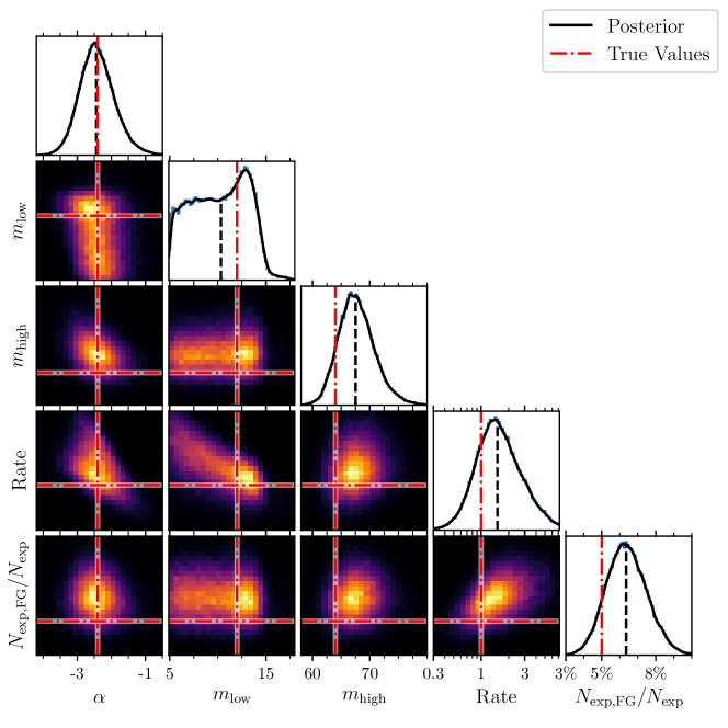
Figure 1: Parameter estimates for a single realisation of the toy model. The foreground population model is a truncated power law with slope $\alpha$, and cut-offs $m_{\mathrm{min}}$ and $m_{\mathrm{max}}$. The expected number of events above the SNR threshold of 8 are 1620, 5% of which are expected to be foreground events. The black lines show the kernel density estimate of the posterior, the thin blue lines the corresponding histogram. The red dash-dotted line indicates the true value for the underlying population.

Our primary results, the estimates of model parameters and their correlations, are shown in figure 1. These results use a SNR threshold 8, the lowest value for which we run our analysis, as we would expect this to yield the best possible parameter estimates. Notable features are the large spread of possible merger rate densities (abbreviated as “Rate”) and their correlation with the lower mass cut-off. This is a consequence of the fact that the power law slope is effectively increased by $3$ due to selection effects, thus detected events are described by a positive slope. The detection bias towards high mass means that fewer events are available to define the lower cut-off value, and low mass events which are observed tend to have lower SNR values. As the total rate is still dominated by low mass (and low-amplitude) events, the large uncertainty of the low mass cut-off yields a high uncertainty on the rate. The estimated fraction of foreground events in the sample of observed events couples linearly to the merger rate density, but is less significant than the lower mass cut-off.

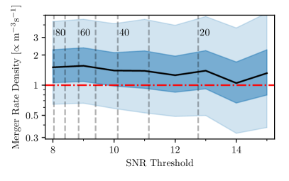
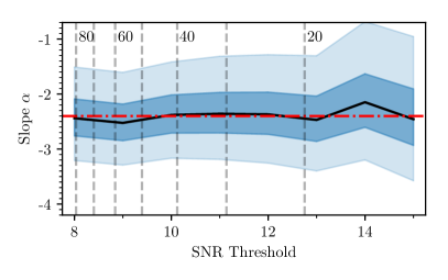
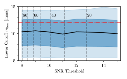
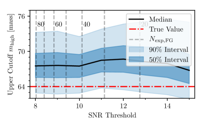
Figure 2: Confidence intervals for individual parameters of one realisation of the truncated power-law model, as a function of SNR threshold. The parameters shown are the inferred astrophysical merger rate (upper left) and power law slope (upper right), as well as the low (lower left) and high (lower right) mass cut-offs. The red dash-dotted line indicates the true value for the underlying population. Dashed grey lines indicate the expected number of foreground events at the given SNR threshold.

To assess our method in the light of its main goal of avoiding bias while lowering the SNR threshold, a single analysis result is insufficient. Therefore, we analyse the same data with a range of different SNR thresholds to observe the change in the hyper-parameter estimates. Figure 2 shows the marginalised posteriors for the rate and power law slope as a function of SNR threshold. We can observe the posteriors growing slightly wider as the SNR threshold is increased and information from fewer events is considered. The result from one single realisation is, however, not necessarily representative of the general behaviour. Combining the results from multiple realisation shows there is no noticeable bias regardless of the threshold chosen, and estimates improve slightly as the threshold is lowered. The width of the 90% credible intervals decreases by factors of $\approx 1.5$ for the power-law slope, $\approx 1.1$ and $\approx 1.05$ for the lower and upper mass cut-offs respectively, and $\approx 1.2$ for the log of the inferred merger rate density.

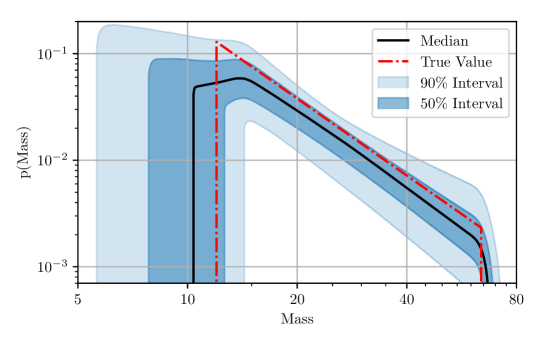
Figure 3: The inferred mass distribution of the foreground population. The bands indicate the given percentiles in the probability density at any given mass across all posterior samples.

Given the estimates of population parameters we can also compute an estimate of the underlying mass distribution, which we show in figure 3. Here we show the $50\%$ and $90\%$ confidence bands, as defined by computing the percentiles of $p(m|\theta)$ across all samples $\theta$ from the posterior for any given mass $m$. We observe that the true distribution is contained well within the credible interval and deviations are generally caused by an underestimated lower cut-off. In general there is a trade-off between expanding the bounds of the mass distribution to include additional events, and shrinking it to increase the PDF for highly significant events. The lower cut-off tends to have more freedom of movement as there are fewer high SNR events at low mass to constrain it.

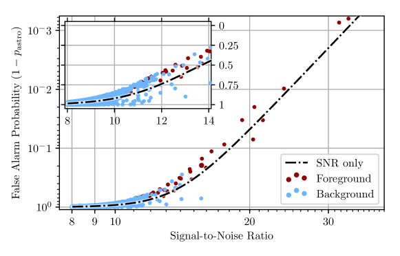
Figure 4: The probability that an event is caused by detector noise rather than being of astrophysical origin, $1-p_{\mathrm{astro}}$, versus SNR. The foreground population model is a truncated power-law distribution. Blue and red dots represent foreground and background events respectively. The dash-dotted line shows the probability that would be inferred by a SNR based estimate Farr et al. (2015), assuming the relative number of expected foreground and background events is known perfectly. The inset focuses on the region with background events and emphasises events which are unlikely to be astrophysical by using a linear scale.

As a final result for this population, figure 4 shows the estimated probability of any given event to have an astrophysical origin $p_{\mathrm{astro}}$, and how it compares to a SNR-only estimate indicated by the black dash-dotted line. While this figure does not show quantitative results, we do observe that foreground events are largely located above the dash-dotted black line, indicating that our confidence in them being real has increased, while background events tend to be located below and are often on the $p_{\mathrm{astro}}=0$ line when their masses are outside the hard cut-offs of the truncated power law population. Thus we find, as expected, that the discrimination between signal and noise populations is improved with the incorporation of information about their mass distributions Dent and Veitch (2014). We determine that the percentage point difference between $p_{\mathrm{astro}}$ using our method and the SNR-only approach to be $\approx 3\%$, although this includes events with tiny absolute shifts due to them being very close to either $0\%$ or $100\%$ in the first place.

IV.2 Gaussian distribution

The second core population considered is a simple Gaussian with a very small width. This population was chosen to test the inference on hard-to-infer parameters and to see the effect a very distinctive distribution has on the discriminating power of our method. As such, we chose the width to be very narrow with a standard deviation of $1.6$ around a mean mass of $27$. This means that the width of the population is smaller than the typical width of the mass posterior of $\approx 2-3$ for each individual event, which we expect to be hard to estimate with a relatively small number of events. On the other hand, the discriminating power of using information from the mass estimates should be much greater than for a wide distribution like the truncated power law used in the previous section.

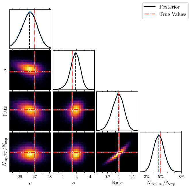
Figure 5: Parameter estimates for a single realisation. The foreground population model is a Gaussian with two free parameters, the mean $\mu$ and width $\sigma$. The true expected numbers of events above a SNR threshold 8 is 1620, $5\%$ of which are expected to be foreground events. The black lines show the kernel density estimate of the posterior, the thin blue lines the corresponding histogram. The red dash-dotted lines indicates the true values for the underlying population.

The parameter estimates for a single realisation are shown in figure 5. We observe that true width of the population $\sigma$ in contained comfortably within the inferred posterior, though the uncertainty is rather large. It is generally overestimated slightly. Similarly the mean of the population is found well with an uncertainty comparable to the population width. The rate is constrained much better than in case of the truncated power law as this model lack the degeneracy between the rate and a poorly constrained population parameter. The lack of a strong correlation between a population parameter and the merger rate density also highlights its linear relation to the estimated number of foreground events contained within the sample.

When lowering the SNR threshold from 15 down to 8, the sizes of the $90\%$ confidence intervals of the population parameters and merger rate density decrease by median factors of $\approx 1.3-1.7$.

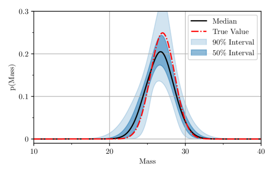
Figure 6: The inferred mass distribution of the foreground population. The bands indicate the given percentiles in the probability density at any given mass across all posterior samples.

The true mass distribution is well within the confidence interval shown in figure 6, though the true distribution is somewhat more narrow than inferred as seen previously in figure 5.

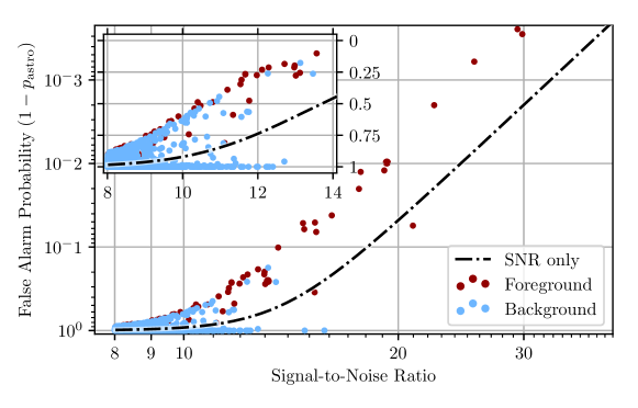
Figure 7: The probability of an event being caused by detector noise rather than being of astrophysical origin, $1-p_{\mathrm{astro}}$, versus SNR. The foreground population model is a narrow Gaussian distribution. Blue and red dots represent foreground and background events respectively. The dash-dotted line shows the probability that would be inferred by a SNR based estimate Farr et al. (2015), assuming the relative number of expected foreground and background events is known perfectly. The inset focuses on the region with background events and emphasises events which are unlikely to be astrophysical by using a linear scale.

The comparison of the estimated $p_{\mathrm{astro}}$ as shown in figure 7 show how important the inclusion of masses is for this population. We can clearly identify the band of foreground events for which $1-p_{\mathrm{astro}}$ is smaller by factors of a few up to 10 compared to the SNR based estimate. Only three out of $\approx 74$ foreground events lost any $p_{\mathrm{astro}}$. There are some background events which, too, have their $p_{\mathrm{astro}}$ increased, though most are demoted and often down to effectively $0$.

IV.3 Incorrect models - No background component

Previous analyses of gravitational wave populations (such as the power law model used in Abbott et al. (2017)) use a high threshold to ensure a high probability that the events used are of astrophysical origin, in effect neglecting the possibility of background. Here we investigate the behaviour of our toy model with the background component disabled, corresponding to such a scenario. This shows the results one would obtain if simply fitting the foreground model to a contaminated dataset. The underlying population is a truncated power law identical to the one used in the first set of results presented in section IV.1.

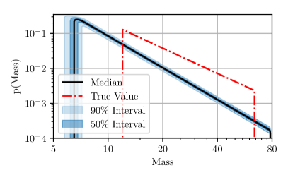
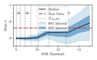
Figure 8: Results for the power law model when we neglect to account for contamination due to noise. Left: Inferred mass distribution at the lowest SNR threshold of 8, the PDF percentiles are calculated across the population posterior at any given mass. Right: Inferred power law slope as a function of SNR threshold. Vertical dashed lines indicate the expected number of true events above a particular SNR.

The results are shown in Fig. 8, where we observe the inferred distribution to be very different from the true one when the lowest SNR threshold of $8$ is used and the dataset is 95% polluted (left panel). The mass cut-offs are extended to the edges of the prior ranges to incorporate noise events at those values. The confidence interval includes the true value as long as the SNR threshold is sufficiently high since the number of background events is negligible, but trends towards $-3$ as the threshold is lowered. This is expected since the background dominates the low SNR region and has a power law slope of $0$ in mass. This slope corresponds to an actual slope of $-3$ when selection effects are considered. In the right panel we see the effect on the estimation of the power law slope as the threshold is varied. At a pollution fraction of 50% (SNR 13.7) the statistical uncertainty of the slope becomes large enough that the systematic bias is not visible.

IV.4 Incorrect models - Neglected selection effects

The second kind of error we considered was the neglect to properly account for the mass dependence of selection effects. In case of a power law distribution this is trivial, as it simply adds $+3$ to the inferred value of the slope. Therefore we chose a Gaussian as the population, and we increased the width to $9$ to highlight the impact of selection effects on the inferred population.

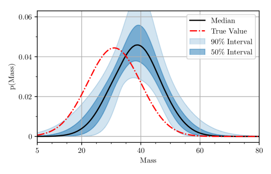
Figure 9: The inferred mass distribution for the Gaussian model without compensating for the mass dependence of selection effects, using the lowest SNR threshold of 8. The PDF percentiles are calculated across the population posterior at any given mass.

Figure 9 shows that the selection effects effectively shift the distribution towards higher masses. This is a general feature as the $m^{3}$ term strongly favours high mass events in the observed set of events. Depending on the population the may also affect the width of the population, which happened to be a very minor effect in this case.

Together with the previous section IV.3 this illustrates that population inference can be made impossible even when the model matches the underlying distribution. Accounting for the presence of noise and selection effects is essential for correct inference and to avoid bias when attempting to lower the SNR threshold.

V Advanced LIGO engineering run

After the successful tests using the simple toy model we also applied this method to more realistic data. For this we used simulated data from the fourth advanced LIGO engineering run (ER4). LIGO Hanford noise data were simulated as Gaussian noise using the LIGO design sensitivity noise spectrum Abbott et al. (2018), while LIGO Livingston data were derived from an instrumental channel monitoring the power-stabilized laser, recoloured to the same average target spectrum. Simulated gravitational wave signals were then added (“injected”) to the recorded noise data streams. The injected population of binary black hole mergers was chosen to be uniform in both component masses between limits of $5$ and $20~{}\mathrm{M}_{\odot}$, and uniform in volume with no cosmological effects included. The EOBNRv2HM approximant tuned to numerical relativity Pan et al. (2011) was used to simulate binary black hole mergers including non-dominant GW emission modes, for non-spinning binary components. The intended astrophysical rate corresponding to the injected merger signals was $5\,\mathrm{Gpc}^{-3}\mathrm{yr}^{-1}$.

We searched the data for signals using the pycbc Dal Canton et al. (2014); Usman et al. (2016); Nitz et al. (2018); Abbott et al. (2016d) pipeline to cover binary mergers of non-spinning components with masses between $3$ and $50~{}\mathrm{M}_{\odot}$; this range also defined the prior for parameter estimation performed on each event using LALinference Veitch et al. (2015). The search detection statistic for candidate events, $\rho_{c}$, is the quadrature sum of $\chi^{2}$-reweighted SNRs $\hat{\rho}_{H,L}$ over single-detector events having consistent component masses and times of arrival between the two detectors Babak et al. (2013); Abadie, J. et al. (2011). The number of events we chose to analyse is limited by computational cost; we impose a threshold $\rho_{c}>8$ leaving us with 100 events in $\approx 37$ days of LHO-LLO coincident observing time; 51 of these events correspond to known injected signals, with the remainder due to noise fluctuations.

We first determine the rates of signal and noise events and the relative probabilities of signal vs. noise origin for each event Farr et al. (2015); Abbott et al. (2016b, c), given only the $\rho_{c}$ value of each event, models of the signal and noise event distributions over $\rho_{c}$, and an estimate of the total rate of noise events derived from time-shifted analyses Babak et al. (2013); Nitz et al. (2018). The result of this estimate is summarized in Fig. 10.

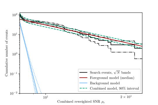
Figure 10: Cumulative number of (simulated) events detected in LIGO ER4 engineering run data vs. threshold search detection statistic $\rho_{c}$. Black steps indicate the search results, with $\pm\sqrt{N}$ bands indicating expected counting fluctuations. Dark red and light blue lines indicate power-law models of signal and noise distributions, respectively. Dotted light blue lines indicate empirical estimates of the noise distribution from each of 3 disjoint analysis periods, showing that the background model $p(\rho_{c}|\eta_{i}\!=\!\mathrm{B})\propto\rho_{c}^{-54.8}$ is sufficiently accurate in the range of interest. Dark green dashed lines show the total expected number of events (signal$+$noise) as a $90\%$ credible band.

We find 53 events with a signal probability $p_{\mathrm{astro}}$ above 50%, of which 47 have $p_{\mathrm{astro}}>90\%$. This analysis is comparable to those used to estimate the rate and $p_{\mathrm{astro}}$ for binary black hole mergers in the first Advanced LIGO Observing period Abbott et al. (2016b), and does not use information about the mass distributions of signal or noise events, besides the assumption that the signal population is contained within the analysis mass limits.

We now turn to our analysis, which estimates the rate and population model parameters simultaneously. The population model used here is a power law in each component mass, of the form

$$p(m_{1},m_{2}|\theta_{\mathrm{F}},\eta_{i}=\mathrm{F})\propto\begin{cases}m_{1}^{\alpha}m_{2}^{\beta}&\mathrm{if}\;m_{\mathrm{low}}<m_{2}\leq m_{1}<m_{\mathrm{high}}\\ 0&\mathrm{else}\end{cases}\\$$ (26)

where $\alpha$ and $\beta$ are the two power law slopes, both with true values equal to $0$. The mass cut-offs $m_{\mathrm{low}}$ and $m_{\mathrm{high}}$ are shared between both power laws, resulting in four free parameters in our population model. The selection effects were simulated numerically using the LALsimulation LIGO Scientific Collaboration implementation of the IMRPhenomPv2 waveform Hannam et al. (2014); Khan et al. (2016) to implement the method described by Finn & Chernoff Finn and Chernoff (1993).

As the background model, we used a power law fit to the distribution of $\rho_{c}$ values from the pycbc time-shifted analysis, giving a slope of $\approx-54.8$ for $\rho_{c}>8$. In a separate step we constructed two dimensional fit to the distribution of component masses in the search results. We find empirically that the background distribution can be approximated as the product of a power-law in chirp mass and a exponential distribution in mass ratio. Using the masses as determined by the search is not strictly the correct approach, which would be to run the time-shifted data through the same LALInference analysis as used for the zero-lag events: this was, though, computationally infeasible. Therefore the search results serve as a proxy for the optimal analysis. We have found empirically that small changes to the background mass distribution do not have a strong effect on the result, which is expected given the dissimilarity of foreground and background distributions. We do not include any additional uncertainty on the background model rate or mass distribution.

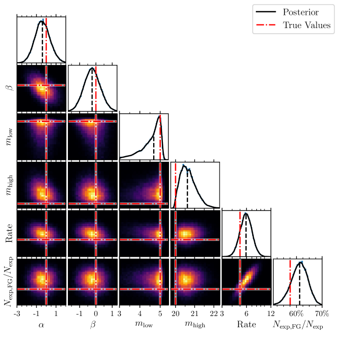
Figure 11: Parameter estimates for the ER4 dataset. The foreground population model is power law in both component masses with separate slopes $\alpha$ and $\beta$ and shared cut-offs $m_{\mathrm{low}}$ and $m_{\mathrm{high}}$. The cut-off masses and merger rate density are given in units of $\mathrm{M}_{\odot}$ and $\mathrm{Gpc}^{-3}\mathrm{yr}^{-1}$ respectively. The black lines show the kernel density estimate of the posterior, the thin blue lines the corresponding histogram. The red dash-dotted line indicates the true value.

The results of estimating the population parameters as displayed in figure 11 show that we successfully recover the true population parameters. The slopes are underestimated slightly which causes the inferred merger rate density to be elevated, although it still encompasses the true value. The mass cut-offs are found well with some tails to lower or higher masses for $m_{\mathrm{low}}$ and $m_{\mathrm{high}}$ respectively, since the uniform distribution of injections covers all regions of the mass range without major gaps and the cut-offs are shared between both component masses.

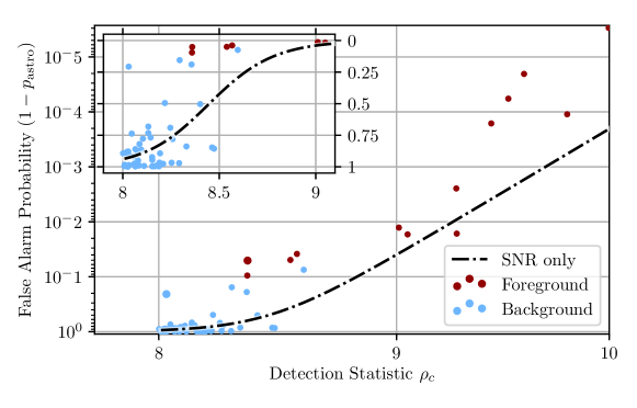
Figure 12: The probability of an event recovered from the ER4 data being caused by noise instead of corresponding to an astrophysical event, which is $1-p_{\mathrm{astro}}$. Blue and red dots represent foreground and background events respectively. The dash-dotted line shows the probability that would be inferred by a SNR based estimate Farr et al. (2015). The inset focuses on the region with background events and emphasises events which are unlikely to be astrophysical by using a linear scale.

Since the slope of the background SNR distribution is much larger than the slope of the astrophysical foreground, the transition region where events may belong to either source category with comparable probabilities is quite small. This means there are few events which fall in between the region of certain background and certain foreground, limiting the gains that can be made by our method in this case. Nevertheless, the fact that the foreground mass distribution is quite distinct from the background causes a significant increase in $p_{\mathrm{astro}}$ relative to the $\rho_{c}$-based approach, as can be seen in figure 12.

As with the previous ranking statistic based analysis we can count the events found with a $p_{\mathrm{astro}}$ value above some given threshold. We find $56$ events above a threshold of $50\%$, which is 3 events more than before. The number of included events which we later identified as noise triggers rises from $4$ to $5$. When the threshold is set to $p_{\mathrm{astro}}>90\%$, the number of events increases by $5$ to $52$, though it now includes one noise trigger. Thus, we find that applying our new method to realistic data not only reproduces the results obtained using established methods, but identifies additional foreground events. We also successfully recover the injected population parameters.

VI Outlook

In this work we have derived a new technique for simultaneous estimation of parameters defining the shape of two or more sub-populations and their expected contribution to the overall number of events. This technique allows us to extract information from formerly sub-threshold events without biasing the result due to uncertainties in classifying their origin. The method is agnostic to the specific choice of threshold, and lowering the threshold will allow more information to be included from events of an uncertain nature, improving the result until the noise completely dominates the signals.

The greatest gains over existing methods are found when there is a large number of events for which the source classification gives comparable probabilities for at least two categories, while the distributions in secondary parameters are very distinct. This behaviour near the transition between populations is likely to be especially useful in the characterisation of weak event populations, such as unresolvable binary mergers at cosmological distances. This is of particular interest when determining whether the source population evolves with redshift. However, this also implies that gains are expected to be small when the primary source classification is very potent and population models are uncertain; in this case our method converges to that with a single population.

While such thresholded analyses that ignore the possible presence of background cannot be guaranteed free of systematic bias, the expected size of bias can be bounded by considering the rate of background events above threshold, as well as the degree of divergence between foreground and background distributions over the parameters of interest. Controlling the bias of a thresholded analysis thus still requires accurate background estimation. In particular, for the small number of events thus far detected by LIGO-Virgo, possible biases on population inference due to neglecting background contamination are expected to be well below statistical errors.

We have successfully tested this new model on different binary merger mass distributions in an artificial universe, as well as to synthetic LIGO data from an engineering run. This demonstrates the feasibility of applying this method to existing and future LIGO-Virgo observing runs, which should allow a better joint determination of source event rates and distributions. The method itself is, however, not limited to the realm of gravitational wave astronomy, and can be useful whenever a set of data points contains multiple populations.

References

- Abbott et al. (2016a) B. P. Abbott et al. (Virgo, LIGO Scientific), Phys. Rev. Lett. 116, 061102 (2016a), arXiv:1602.03837 [gr-qc] .
- Abbott et al. (2016b) B. P. Abbott et al. (Virgo, LIGO Scientific), Phys. Rev. X 6, 041015 (2016b), arXiv:1606.04856 [gr-qc] .
- Abbott et al. (2016c) B. P. Abbott et al. (Virgo, LIGO Scientific), Astrophys. J. 833, L1 (2016c), arXiv:1602.03842 [astro-ph.HE] .
- Abbott et al. (2018) B. P. Abbott et al., Living Reviews in Relativity 21, 3 (2018).
- Abbott et al. (2016d) B. P. Abbott et al. (Virgo, LIGO Scientific), Phys. Rev. D93, 122003 (2016d), arXiv:1602.03839 [gr-qc] .
- Usman et al. (2016) S. A. Usman, A. H. Nitz, I. W. Harry, C. M. Biwer, et al., Class. Quant. Grav. 33, 215004 (2016), arXiv:1508.02357 [gr-qc] .
- Cannon et al. (2012) K. Cannon, R. Cariou, A. Chapman, M. Crispin-Ortuzar, et al., Astrophys. J. 748, 136 (2012), arXiv:1107.2665 [astro-ph.IM] .
- Cannon et al. (2015) K. Cannon, C. Hanna, and J. Peoples, ArXiv e-prints (2015), arXiv:1504.04632 [astro-ph.IM] .
- Messick et al. (2017) C. Messick, K. Blackburn, P. Brady, P. Brockill, et al., Phys. Rev. D95, 042001 (2017), arXiv:1604.04324 [astro-ph.IM] .
- Nitz et al. (2017) A. H. Nitz, T. Dent, T. Dal Canton, S. Fairhurst, and D. A. Brown, Astrophys. J. 849, 118 (2017), arXiv:1705.01513 [gr-qc] .
- Allen (2005) B. Allen, Phys. Rev. D 71, 062001 (2005), arXiv:gr-qc/0405045 [gr-qc] .
- Nitz (2018) A. H. Nitz, Class. Quant. Grav. 35, 035016 (2018), arXiv:1709.08974 [gr-qc] .
- Capano et al. (2017) C. Capano, T. Dent, C. Hanna, M. Hendry, et al., Phys. Rev. D 96, 082002 (2017).
- Abbott et al. (2016e) B. P. Abbott et al. (Virgo, LIGO Scientific), Class. Quant. Grav. 33, 134001 (2016e), arXiv:1602.03844 [gr-qc] .
- Fairhurst and Brady (2008) S. Fairhurst and P. Brady, Class. Quant. Grav. 25, 105002 (2008), arXiv:0707.2410 [gr-qc] .
- Tiwari (2017) V. Tiwari, (2017), arXiv:1712.00482 [astro-ph.HE] .
- Ng et al. (2018) K. K. Y. Ng, S. Vitale, A. Zimmerman, K. Chatziioannou, D. Gerosa, and C.-J. Haster, (2018), arXiv:1805.03046 [gr-qc] .
- Farr et al. (2015) W. M. Farr et al., Phys. Rev. D 91, 023005 (2015), arXiv:1302.5341 [astro-ph.IM] .
- Smith and Thrane (2018) R. Smith and E. Thrane, Phys. Rev. X8, 021019 (2018), arXiv:1712.00688 [gr-qc] .
- Li et al. (2012) T. G. F. Li, W. Del Pozzo, S. Vitale, C. Van Den Broeck, et al., Phys. Rev. D85, 082003 (2012), arXiv:1110.0530 [gr-qc] .
- Del Pozzo et al. (2013) W. Del Pozzo, T. G. F. Li, M. Agathos, C. Van Den Broeck, and S. Vitale, Phys. Rev. Lett. 111, 071101 (2013), arXiv:1307.8338 [gr-qc] .