Neutron Star Mergers Are the Dominant Source of the r-process in the Early Evolution of Dwarf Galaxies

Abstract

There are many candidate sites of the $r$-process: core-collapse supernovae (including rare magnetorotational core-collapse supernovae), neutron star mergers, and neutron star/black hole mergers. The chemical enrichment of galaxies—specifically dwarf galaxies—helps distinguish between these sources based on the continual build-up of $r$-process elements. This technique can distinguish between the $r$-process candidate sites by the clearest observational difference—how quickly these events occur after the stars are created. The existence of several nearby dwarf galaxies allows us to measure robust chemical abundances for galaxies with different star formation histories. Dwarf galaxies are especially useful because simple chemical evolution models can be used to determine the sources of $r$-process material. We have measured the $r$-process element barium with Keck/DEIMOS medium-resolution spectroscopy. We present the largest sample of barium abundances (almost 250 stars) in dwarf galaxies ever assembled. We measure [Ba/Fe] as a function of [Fe/H] in this sample and compare with existing [$\alpha$/Fe] measurements. We have found that a large contribution of barium needs to occur at more delayed timescales than core-collapse supernovae in order to explain our observed abundances, namely the significantly more positive trend of the $r$-process component of [Ba/Fe] vs. [Fe/H] seen for $\text{[Fe/H]}\lesssim-1.6$ when compared to the [Mg/Fe] vs. [Fe/H] trend. We conclude that neutron star mergers are the most likely source of $r$-process enrichment in dwarf galaxies at early times.

1 Introduction

The premise of galactic archeology is that stars form out of a galaxy’s gas and adopt the chemical composition of the gas when they were born. At the same time, galactic inflows, outflows, and stellar ejecta dilute or enhance the chemical composition in a galaxy. We can not watch these processes happen in real time in an individual galaxy, so instead we use galactic archeology to learn how a given galaxy has evolved. Galactic archeology looks back in time by utilizing the fact that long-lived stars retain the memory of the chemical composition of the galaxy when they were born. We trace a variety of elements in stars alive today to learn about the timescales and origins of chemical enrichment in dwarf galaxies.

We will discuss three different groups of elements observable in stars. These elements were chosen because each group traces different stellar events. The first group is the $\alpha$ elements (e.g., Mg). These elements are created and ejected in core-collapse supernovae (CCSNe) with a short delay time ($4-25$ Myr). The delay time is defined as the time between the star being born and the star ejecting enriched material into the ISM. The second group is iron. Iron is produced in large amounts by SNe Ia with a relatively long delay time ($0.04-14$ Gyr, Maoz & Graur, 2017) described by a delay time distribution. In addition, there are moderate amounts of iron that are generated in each CCSNe. Finally, elements heavier than iron are formed through neutron-capture processes. Determining the dominant origin of neutron-capture elements is still an active area of study and is the focus of this paper. Because the origin is unknown, the delay time is also unknown.

The ratio of $\alpha$ elements to iron ([$\alpha$/Fe]) is commonly used as a chemical clock (Tinsley, 1980). If we know the exact amount of each element released during each process (also referred to as the yield), [$\alpha$/Fe] can tell us the ratio of CCSNe to SNe Ia as a function of time. Starting from a star formation history (SFH), one can convert time into an iron abundance by assuming an initial mass function (IMF) and supernovae iron yields. As a stellar population ages, the rate of CCSNe changes compared to SNe Ia because of their different lifetimes. The [$\alpha$/Fe] starts out high at low [Fe/H] (or early times) because CCSNe quickly eject a large amount of $\alpha$ elements with small amounts of iron (Nomoto et al., 2006). Then [$\alpha$/Fe] dramatically declines as time passes and [Fe/H] increases, because SNe Ia start to explode and eject large amounts of iron (Iwamoto et al., 1999). The plot of [$\alpha$/Fe] vs. [Fe/H] has been used in many studies of galactic evolution, typically by using [Mg/Fe] as an indicator of the total [$\alpha$/Fe] (e.g., Gilmore & Wyse, 1991; Shetrone et al., 2001; Venn et al., 2004; Kirby et al., 2011a; Bensby et al., 2014).

Using neutron-capture elements as a chemical clock is less common, but may be the key to distinguish the dominant origin of neutron-capture elements. This paper uses barium as a tracer of all neutron-capture elements, because barium is arguably the easiest neutron-capture element to measure due to its several strong absorption lines available in the optical. The [Ba/Fe] indicates what levels of barium are being ejected into the ISM compared to SNe Ia throughout time. Combining the [Ba/Fe] vs. [Fe/H] ‘chemical clock’ with abundances of another neutron-capture element (e.g., europium), clarifies the origin of neutron-capture elements even further. The ratio of these two different neutron-capture elements ([Ba/Eu]) tells us the percentage of all neutron-capture elements produced by the two different neutron-capture processes: the $s$- and the $r$-process.

The slow neutron-capture process ($s$-process) and the rapid neutron-capture process ($r$-process) occur in very different physical scenarios and originate in very different astrophysical origins. The $s$-process occurs in episodes lasting from $10^{2}-10^{4}$ yrs. The $s$-process has a very long time between each free neutron being captured ($\tau_{\text{n}}\sim 10-10^{4}$ yr), and this timescale is much longer than the timescale for that neutron to $\beta$-decay into a proton. We know that for heavy neutron-capture elements—such as barium—the $s$-process is produced by AGB stars, with trace amounts possibly produced in massive stars (e.g., Karakas & Lattanzio, 2014).

The $r$-process occurs in a single event that lasts seconds and an isotope can capture many neutrons ($\tau_{\text{n}}\sim 10^{-2}-10$ sec) before those neutrons $\beta$-decay into a proton. Unlike the $s$-process, there is little consensus on the astrophysical origin of the $r$-process, but the origin has been isolated to various explosions or mergers. We will now use the results of theoretical models and observational constraints to limit our search for the dominant $r$-process origin.

1.1 Narrowing Down the Search for the Dominant R-Process Origin

Arguably the largest gap in our knowledge of stellar nucleosynthesis is the origin of heavy elements that are produced by the $r$-process. Specifically, CCSNe, magnetorotational supernovae (MRSNe), common envelope jets SNe, binary neutron star mergers (NSMs), and neutron star/black hole mergers (NS+BHs) are currently being considered (e.g., Arnould et al., 2007; Thielemann et al., 2011; Papish et al., 2015; Liccardo et al., 2018).

In a CCSN it was thought that neutrino winds drive neutrons and protons from the surface of the proto-neutron star (located at the core), resulting in a large neutron flux in the middle region of the explosion, which might be a site of $r$-process (Woosley & Janka, 2005). However, recent simulations have been unable to generate $r$-process elements up to or beyond barium except in extreme cases (e.g., Wanajo, 2013). This limitation on the average $r$-process yields of CCSNe provided by simulations paired with estimates of the yield required by observations has convincingly eliminated ‘typical’ CCSNe as the dominant source of the $r$-process (e.g., Macias & Ramirez-Ruiz, 2016).

However, rare types of CCSNe that produce copious amounts of $r$-process material are still being considered as a potential source of $r$-process. MRSNe are supernovae that start out with high magnetic fields (B$\sim 10^{12-13}$ G) that cause jet-like explosions, which may produce $r$-process elements. MRSNe are possibly $0.1\%-1\%$ of all CCSNe and could produce enough $r$-process material to account for the observed levels of $r$-process enrichment found in the solar system. Simulations have been able to reproduce the full $r$-process pattern seen in the solar system with only minor discrepancies (Mösta et al., 2017; Nishimura et al., 2015, 2017). There is currently no proof that MRSNe occur, although it is the most popular explanation for hydrogen-poor superluminous supernovae (SLSNe I, e.g., Kasen & Bildsten, 2010; De Cia et al., 2018). This lack of observational constraints means that there is also no proof that MRSNe actually produce large amounts of $r$-process material.

Another rare type of SN is a common envelope jets SN (Papish et al., 2015; Soker & Gilkis, 2017). In this scenario, the primary star in a binary system evolves into a neutron star. When the secondary becomes a red supergiant, it subsumes the neutron star, which spirals into the giant. If the neutron star makes it to the core, it can launch jets and form an accretion disk, possibly including $r$-process nucleosynthesis (Grichener & Soker, 2018). This type of SN would have a delay time slightly longer than a CCSN but shorter than a NSM.

NSMs have the most complete theoretical models and easily produce a large amount of $r$-process material. Simulations have predicted that NSMs are able to recreate the full $r$-process pattern (including barium), and have shown that these results are insensitive to the detailed choices of the simulation (Côté et al., 2017). NSMs now have an observational constraint in the form of the first observed neutron star merger (GW170817, Abbott et al., 2017). The discovery of the electro-magnetic counterpart was originally announced by Coulter et al. (2017). Photometric and spectral follow-up enabled $r$-process yields to be determined (Tanvir et al., 2017; Troja et al., 2017; Evans et al., 2017). This is the first observational constraint of an $r$-process yield coming from a known astrophysical origin. This NSM yield is high enough for all $r$-process elements to be produced by NSMs. However, assuming the yield from GW170817 is an accurate average of all NSMs could be inaccurate. Quantitative predictions for the rates, time delays, and yields are still active areas of study (e.g., Radice et al., 2016).

Some NS+BHs likely reproduce the full $r$-process pattern as well, but restrictions (e.g., on the black hole mass and spin) are required to eject $r$-process material from a NS+BHs (e.g., Lattimer & Schramm, 1974; Shibata & Taniguchi, 2011; Foucart et al., 2015; Barack et al., 2018). The subset of NS+BHs that are a source of $r$-process are expected to be much rarer than the NSMs. Therefore, the contribution of neutron star–neutron star mergers dominates over the contribution of neutron star–black hole mergers.

We have narrowed down our search for the dominant source of $r$-process enrichment in galaxies to a rare form of core-collapse supernovae (i.e., MRSNe) or NSMs. The simulations of these two candidate sites are so poorly constrained that distinguishing between MRSNe and NSMs by comparing detailed abundance patterns is extremely challenging (e.g., Ji & Frebel, 2018). The clearest way to definitively distinguish between MRSNe and NSMs is by their different timescales.

1.2 Distinguishing Between Dominant R-Process Candidates Based on Timescales for the First Time

The chemical enrichment of galaxies—specifically dwarf galaxies—enables us to distinguish between these sources based on their timescales. This is possible because we observe the continual build-up of $r$-process elements, and this type of study is an essential counterpart to the characterization of individual events. Specifically, we are sensitive to the enrichment timescale, which is the key distinguishing characteristic between MRSNe and NSMs. Robust chemical abundance trends can be measured for nearby dwarf galaxies, because their nearness and intact stellar populations allow us to average the abundances of many individually resolvable stars. Determining the sources of chemical enrichment from our observed abundance trends in dwarf galaxies is possible, because (1) their small masses make them very sensitive to feedback mechanisms, (2) the lack of major mergers helped preserve their stellar populations, and (3) their small sizes result in nearly instantaneous mixing compared to the chemical enrichment timescale (Escala et al., 2018). All of these properties make dwarf galaxies the perfect test sites to observe the simplest form of galactic chemical evolution. The existence of several nearby dwarf galaxies provides additional diagnostic power, because we can measure the chemical enrichment for galaxies with different star formation histories. The lessons learned in dwarf galaxies can then be applied to larger, more complex galaxies.

The usefulness of dwarf galaxies for determining the characteristics of $r$-process enrichment can be seen in Ji et al.’s 2016 study of the ultra-faint dwarf (UFD) galaxy Reticulum II. Several stars in Reticulum II have very high levels of enrichment in barium and europium. No other similarly enhanced stars were found in the other nine UFD galaxies considered. This indicates that a rare event occurred that dramatically increased the neutron-capture enrichment in Reticulum II. The [Ba/Eu] confirms that this enrichment was created by the $r$-process. Ji et al. (2016) calculated that this high enrichment could be caused by a single event in the small UFD galaxy. This rules out a typical CCSN, because CCSNe are so frequent that we would see this effect in many UFD galaxies (also see Beniamini et al., 2016b, 2018). Both MRSNe and NSMs are predicted to be rare and produce a large amount of $r$-process enrichment. As we have mentioned before, the main observable difference between MRSNe and NSMs is their timescales. The short SFH of Reticulum II challenges whether it is possible to have a NSM occur while stars are still forming. However, because we are discussing a single rare event, it is possible an unusually quick NSM occurred in Reticulum II. Therefore we need to see enrichment occur in larger mass dwarf galaxies, so that many of these rare prolific $r$-process events have occurred and we have some statistical certainty if we need an event with a short (MRSNe) or long (NSMs) timescale.

In order to break this degeneracy between NSMs and MRSNe, we need a large sample of stars in many moderately-sized dwarf galaxies. We have measured barium with DEIMOS medium-resolution spectroscopy (Faber et al., 2003), and will present the largest sample of barium abundances (almost 250 stars) in dwarf galaxies ever assembled.

1.3 Abundance Measurements from Medium-Resolution Multi-Object Spectroscopy

A large number of stars is needed to distinguish the chemical trend of a stellar population from star-to-star variations. We were able to obtain a large sample of stars, because we used multi-object, medium-resolution spectroscopy (MRS, R $\approx 5,000$). Typically barium is measured using high-resolution spectroscopy (HRS, R $>20,000$) on single-slit spectrographs. Traditionally, precise chemical abundance measurements required equivalent width measurements of absorption lines in HRS, and because of this the Dwarf Abundances and Radial velocities Team (DART; Tolstoy et al., 2006) invested the necessary observing time to obtain HRS for tens of individual stars in Sculptor and Fornax (e.g., Lemasle et al., 2014; Starkenburg et al., 2013). To obtain a large sample of stars with moderate observing time, we used MRS which enables tens of member stars to be observed simultaneously.

The main weakness of MRS is increased line blending. The blending that occurs in MRS causes strong sky lines to contaminate a larger range of wavelengths, the continuum to be obscured, and the apparent weakening of absorption lines. Since blending prevents the continuum from being measured in the gaps between absorption/emission lines, the continuum is iteratively fitted while the abundances are measured using the synthetic spectra.

We overcome these weaknesses to take advantage of higher S/N per pixel or fainter limiting magnitude that can be achieved with a given amount of observation time ($V\lesssim 20$ mag compared to 18 mag for HRS), which increases the sample of observable red giant branch stars. Wider spectral coverage increases the number of absorption lines observed per chemical element, which is especially important for elements with few clear absorption lines (e.g., neutron-capture elements). For barium, we use five different absorption lines in our measurements.

Both HRS and MRS require a stellar atmosphere model and stellar line analysis—either to measure abundances from equivalent widths or to generate synthetic spectra. Common simplifications for both methods are to use a one-dimensional (1D) stellar atmosphere model and to assume local thermodynamic equilibrium (LTE) throughout the star. Correcting for 3D and non-LTE effects could systematically shift barium abundance measurements by 0.1–0.3 dex (see Section 4.1), similar to the statistical uncertainties of our measurements. Unfortunately, both of these corrections are very computationally intensive and are beyond the scope of this project.

Determining chemical abundances from MRS has returned uncertainties as low as 0.1 dex for iron and $\alpha$ elements in dwarf galaxies (Kirby et al., 2010). This paper will demonstrate that we can also achieve similar uncertainties for barium abundances in dwarf galaxies. Therefore, we are able to use a multi-object spectrographs MRS without sacrificing accuracy to obtain barium abundances for a large sample of stars.

2 Observations

We observed a diverse sample of dwarf galaxies to probe what [Ba/Fe] measurements can tell us about the chemical enrichment mechanisms and SFHs in different galaxies. Our sample includes five classical dwarf spheroidal galaxies: Fornax, Sculptor, Sextans, Draco, and Ursa Minor. These galaxies span a variety of masses (M${}_{\ast}\sim 10^{5}-10^{7}$ M_⊙) and durations of star formation ($\approx 1$–$11$ Gyr of star formation, Weisz et al. 2014). In each of these galaxies we obtained MRS for individual red giant branch stars using DEIMOS on Keck II.

Apart from these galaxies, we also observed red giant branch stars in globular clusters and the halo of the Milky Way to compare our [Ba/Fe] measurements to those found in the literature. This comparison is used to estimate our systematic error (see Section 4.2).

The locations and distances to all spectroscopic targets are listed in Table 2. The details of all observations contained in this paper are given in Table 2. This includes the name of the slitmask, number of slits, date, airmass, seeing, and exposure time of all observations. This table also includes references for star selection and membership verification.

Table 1: Spectroscopic Targets

Target	RA	Dec	D	$(m-M)_{0}$
	(J2000)	(J2000)	(kpc)	(mag)
Globular Clusters
NGC 2419	$07^{\mathrm{h}}38^{\mathrm{m}}09^{\mathrm{s}}$	$+38\arcdeg 52\arcmin 55\arcsec$	082.6	19.83
NGC 4590 (M68)	$12^{\mathrm{h}}39^{\mathrm{m}}28^{\mathrm{s}}$	$-26\arcdeg 44\arcmin 39\arcsec$	010.3	15.21
NGC 6341 (M92)	$17^{\mathrm{h}}17^{\mathrm{m}}07^{\mathrm{s}}$	$+43\arcdeg 08\arcmin 11\arcsec$	008.3	14.65
NGC 7078 (M15)	$21^{\mathrm{h}}29^{\mathrm{m}}58^{\mathrm{s}}$	$+12\arcdeg 10\arcmin 01\arcsec$	010.4	15.39
Halo Field Stars
BD $+$14 550	$03^{\mathrm{h}}18^{\mathrm{m}}27^{\mathrm{s}}$	$+15\arcdeg 10\arcmin 38\arcsec$
BD $-$00 552	$03^{\mathrm{h}}28^{\mathrm{m}}54^{\mathrm{s}}$	$-00\arcdeg 25\arcmin 03\arcsec$
BD +22 626	$04^{\mathrm{h}}04^{\mathrm{m}}11^{\mathrm{s}}$	$+23\arcdeg 24\arcmin 27\arcsec$
BD $-$13 942	$04^{\mathrm{h}}38^{\mathrm{m}}56^{\mathrm{s}}$	$-13\arcdeg 20\arcmin 48\arcsec$
BD $-$14 1399	$06^{\mathrm{h}}18^{\mathrm{m}}49^{\mathrm{s}}$	$-14\arcdeg 50\arcmin 43\arcsec$
BD $+$62 959	$07^{\mathrm{h}}54^{\mathrm{m}}29^{\mathrm{s}}$	$+62\arcdeg 08\arcmin 11\arcsec$
BD $+$80 245	$08^{\mathrm{h}}11^{\mathrm{m}}06^{\mathrm{s}}$	$+79\arcdeg 54\arcmin 30\arcsec$
BD $+$21 1969	$09^{\mathrm{h}}06^{\mathrm{m}}43^{\mathrm{s}}$	$+20\arcdeg 30\arcmin 36\arcsec$
BD $-$20 2955	$09^{\mathrm{h}}36^{\mathrm{m}}20^{\mathrm{s}}$	$-20\arcdeg 53\arcmin 15\arcsec$
BD $+$55 1362	$10^{\mathrm{h}}04^{\mathrm{m}}43^{\mathrm{s}}$	$+54\arcdeg 20\arcmin 43\arcsec$
BD $+$54 1359	$10^{\mathrm{h}}14^{\mathrm{m}}29^{\mathrm{s}}$	$+53\arcdeg 33\arcmin 39\arcsec$
BD $+$40 2408	$11^{\mathrm{h}}13^{\mathrm{m}}55^{\mathrm{s}}$	$+39\arcdeg 58\arcmin 40\arcsec$
BD $-$04 3155	$11^{\mathrm{h}}51^{\mathrm{m}}50^{\mathrm{s}}$	$-05\arcdeg 45\arcmin 44\arcsec$
BD $+$49 2098	$11^{\mathrm{h}}58^{\mathrm{m}}00^{\mathrm{s}}$	$+48\arcdeg 12\arcmin 12\arcsec$
BD $+$09 2653	$12^{\mathrm{h}}40^{\mathrm{m}}14^{\mathrm{s}}$	$+08\arcdeg 31\arcmin 38\arcsec$
dSphs
Sculptor	$01^{\mathrm{h}}00^{\mathrm{m}}09^{\mathrm{s}}$	$-33\arcdeg 42\arcmin 32\arcsec$	085.0	19.67
Fornax	$02^{\mathrm{h}}39^{\mathrm{m}}59^{\mathrm{s}}$	$-34\arcdeg 26\arcmin 57\arcsec$	139.0	20.72
Sextans	$10^{\mathrm{h}}13^{\mathrm{m}}03^{\mathrm{s}}$	$-01\arcdeg 36\arcmin 52\arcsec$	095.0	19.90
Ursa Minor	$15^{\mathrm{h}}09^{\mathrm{m}}11^{\mathrm{s}}$	$+67\arcdeg 12\arcmin 52\arcsec$	069.0	19.18
Draco	$17^{\mathrm{h}}20^{\mathrm{m}}19^{\mathrm{s}}$	$+57\arcdeg 54\arcmin 48\arcsec$	092.0	19.84

References. — See Harris (1996, 2010 edition, http://www.physics.mcmaster.ca/~harris/mwgc.dat) and references therein for the coordinates and distances for the globular clusters. Halo field stars coordinates are from Fulbright (2000). The remaining dSph coordinates are adopted from Mateo (1998), and the distances are adopted from the following sources: Sculptor, Pietrzyński et al. (2008); Fornax, Rizzi et al. (2007); Sextans, Lee et al. (2003); Ursa Minor, Mighell & Burke (1999); Draco, Bellazzini et al. (2002).

Table 2: DEIMOS Observations

Object	Slitmask	Reference	# targets	Date			Airmass	Seeing	Exposures
Globular Clusters
NGC 2419	n2419b	Kirby et al. (2016)	112	2012	Mar	19	1.07	$0\farcs 74$	3 $\times$ 900 s
NGC 4590 (M68)	n4590a	Kirby et al. (2016)	096	2014	Feb	2	1.60	$0\farcs 80$	1200 s, 937 s
NGC 6341 (M92)	6341l1	Kirby et al. (2016)	177	2017	Mar	28	1.20	$0\farcs 71$	6 $\times$ 1800 s, 2000 s
NGC 7078 (M15)	n7078d	Kirby et al. (2016)	164	2011	Jul	29	1.03	$1\farcs 10$	3 $\times$ 600 s
	n7078e	Kirby et al. (2016)	167	2011	Jul	30	1.05	$0\farcs 86$	3 $\times$ 900 s
Halo Field Stars
BD $+$14 550	LVMslits	Fulbright (2000)	001	2016	Dec	30	1.18	$>1\farcs 5$	300 s
BD $-$00 552	LVMslits	Fulbright (2000)	001	2016	Dec	30	1.14	$>1\farcs 5$	600 s
BD +22 626	LVMslits	Fulbright (2000)	001	2016	Dec	30	1.05	$>1\farcs 5$	600 s
BD $-$13 942	LVMslits	Fulbright (2000)	001	2016	Dec	30	1.20	$>1\farcs 5$	300 s
BD $-$14 1399	LVMslits	Fulbright (2000)	001	2016	Dec	30	1.26	$>1\farcs 5$	2 $\times$ 300 s
BD $+$62 959	LVMslits	Fulbright (2000)	001	2016	Dec	30	1.35	$>1\farcs 5$	300 s
BD $+$80 245	LVMslits	Fulbright (2000)	001	2016	Dec	30	1.99	$>1\farcs 5$	2 $\times$ 600 s
BD $+$21 1969	LVMslits	Fulbright (2000)	001	2016	Dec	30	1.12	$>1\farcs 5$	300 s
BD $-$20 2955	LVMslits	Fulbright (2000)	001	2016	Dec	30	1.35	$>1\farcs 5$	300 s
BD $+$55 1362	LVMslits	Fulbright (2000)	001	2016	Dec	30	1.26	$>1\farcs 5$	2 $\times$ 300 s
BD $+$54 1359	LVMslits	Fulbright (2000)	001	2016	Dec	30	1.28	$>1\farcs 5$	2 $\times$ 300 s
BD $+$40 2408	LVMslits	Fulbright (2000)	001	2016	Dec	30	1.08	$>1\farcs 5$	300 s
BD $-$04 3155	LVMslits	Fulbright (2000)	001	2016	Dec	30	1.32	$>1\farcs 5$	300 s
BD $+$49 2098	LVMslits	Fulbright (2000)	001	2016	Dec	30	1.18	$>1\farcs 5$	300 s
BD $+$09 2653	LVMslits	Fulbright (2000)	001	2016	Dec	30	1.25	$>1\farcs 5$	300 s
dSphs
Sculptor	bscl1	Kirby et al. (2009)	086	2011	Jul	31	1.72	$0\farcs 75$	4 $\times$ 1200 s, 900 s
	bscl2	Kirby et al. (2009)	106	2011	Aug	6	1.82	$0\farcs 74$	2 $\times$ 1200 s, 2 $\times$ 840 s
	bscl6	Kirby et al. (2009)	091	2011	Aug	4	1.72	$0\farcs 83$	4 $\times$ 1200 s
Fornax	bfor6	Kirby et al. (2010)	169	2011	Aug	5	1.86	$1\farcs 26$	2 $\times$ 800 s
				2011	Aug	6	1.83	$0\farcs 76$	1200 s
				2011	Aug	7	1.90	$0\farcs 83$	3 $\times$ 1200 s
Sextans	bsex2	Kirby et al. (2010)	085	2016	Jan	30	1.10	$\cdots$	2 $\times$ 1800 s
				2016	Jan	31	1.11	$\cdots$	2 $\times$ 1800 s, 1000 s
	bsex3	Kirby et al. (2010)	085	2016	Jan	29	1.55	$\cdots$	6 $\times$ 1550 s
Ursa Minor	bumi1	Kirby et al. (2010)	125	2011	Jul	29	1.52	$0\farcs 57$	600 s, 4 $\times$ 1200 s
	bumi2	Kirby et al. (2010)	134	2011	Jul	31	1.68	$0\farcs 73$	4 $\times$ 1200 s
	bumi3	Kirby et al. (2010)	137	2011	Aug	4	1.80	$0\farcs 64$	4 $\times$ 1200 s
Draco	bdra1	Kirby et al. (2010)	151	2011	Jul	30	1.42	$1\farcs 18$	5 $\times$ 1200 s
	bdra2	Kirby et al. (2010)	167	2011	Aug	7	1.28	$0\farcs 67$	4 $\times$ 1200 s
	bdra3	Kirby et al. (2010)	140	2011	Aug	5	1.37	$0\farcs 98$	5 $\times$ 1200 s

2.1 Star Selection and Member Verification

We relied on the star selection, member verification, and stellar parameters found in the literature. The details of how these stars were selected and how membership was determined are found in the references listed in Table 2. Here we outline these methods in two groups, which are separated by the concentration of the desired stars: targets observed with A) multi-object or B) single-object slitmasks.

A) Multi-object slitmasks were used to observe all dwarf galaxies and globular clusters. In general, multi-object slitmasks were designed using the dsimulator software package. Stars were prioritized to be included on the slitmask based on their overall brightness and the likelihood they are on the red giant branch—determined using their surface gravity ($\log g$) and position on the color–magnitude diagram. The stars were then verified as members of the galaxy or globular cluster based on radial velocity measurements.

B) Single slit spectroscopy was used to obtain observations of Milky Way halo stars. Halo stars were selected from Fulbright (2000), who verified that the stars belonged to the Milky Way halo using proper motion measurements. To exclude dwarf stars from our sample, we applied an additional constraint by only including stars with $\log g$ $<3.6$, adopting Fulbright’s measurements of surface gravity.

2.2 Spectroscopic Configuration and Reduction

Previous work (e.g., Kirby et al. 2010) utilized the 1200 lines mm^-1 DEIMOS grating from 6400–9000 Å (with a spectral resolution of $R\approx 6500$ at $8500$ Å with $0\farcs 7$ slits). However, the optical barium absorption lines are bluer (4554–6497 Å) than can be observed efficiently with this grating, which has a blaze wavelength of 7760 Å. Therefore, to measure individual barium abundances for each star, we chose a lower resolution grating that allowed bluer wavelengths to be observed. We used the 900ZD DEIMOS grating (900 lines mm^-1), which has a blaze wavelength of 5500 Å. This configuration can yield up to 80–150 spectra per slitmask with medium resolution ($\approx 1.96$ Å FWHM or R $\approx 2550$ at $5000$ Å with $0\farcs 7$ slits). A central wavelength of $5500$ Å coupled with an order-blocking filter (GG400) results in a spectral range of 4000–7200 Å. Kr, Ne, Ar, and Xe arc lamps were used for wavelength calibration, and a quartz lamp was used for flat fielding.

We reduced all observations using the spec2d pipeline (Newman et al., 2013; Cooper et al., 2012). This pipeline automatically determines the wavelength solution using the spectral arcs. However, these wavelength solutions were not sufficiently accurate, because the arc lamps have few detectable emission lines with wavelengths less than $\approx 5000$ Å at the exposure times that we used. To improve the wavelength solution, synthetic spectra were generated and cross-correlated against the observed spectra at H$\alpha,H\beta,$ and H$\gamma$ in windows of 20Å. A line was fit to establish the wavelength correction ($\Delta\lambda$) as a function of wavelength ($\lambda$). This solution precludes the ability to measure absolute radial velocities, but our only focus for this work is to measure barium abundances.

We corrected for the global continuum by first fitting a spline to the observed spectrum with a break point every 200 pixels (88 Å) with an upper and lower threshold of $5\sigma$ and $0.1\sigma$, respectively. Then, we divided the observed spectrum by the resulting spline fit to correct for the global continuum. We later refine the local continuum determination during the barium abundance measurements (Section 3.2).

3 Barium Abundance Measurements

We measure barium abundances by first adopting stellar parameter measurements found in the literature, specifically the effective temperature ($T_{\rm{eff}}$), surface gravity ($\log g$), metallicity ([Fe/H]), and $\alpha$-to-iron ratio ([$\alpha$/Fe]). Abundances presented in this paper are referenced to solar (e.g., [Fe/H] $=($Fe/H$)_{\ast}-($Fe/H$)_{\odot}$). Our definition of the solar elemental abundances can be found in Table 3.

Table 3: Adopted Solar Composition

Element	(X/H) = 12 + $\log\epsilon_{X}$
Mg	7.58
Fe	7.52
Ba	2.13
Eu	0.51

Note. — Solar abundances are from Anders & Grevesse (1989), except for iron which is from Sneden et al. (1992). Elemental abundance is defined as: (X/H) $=12+\log\epsilon_{X}=12+\log(n_{X})-\log(n_{H})$.

For dwarf galaxies and globular clusters, we adopted the parameter measurements from Kirby et al. (2010) and Kirby et al. (2016), respectively. See Kirby et al. (2010, 2016) for a full description of those measurements, which we briefly summarize here. The surface gravity and initial value of $T_{\rm{eff}}$ were estimated from photometry. Then $T_{\rm{eff}}$, [Fe/H], and [$\alpha$/Fe] were measured by matching the synthetic spectra to the observed spectra. The microturbulent velocity ($\xi$) of the stellar atmosphere was calculated from the surface gravity (Equation 1).

$$\xi(\text{km\,s}^{-1})=(2.13\pm 0.05)-(0.23\pm 0.03)\log g$$ (1)

For Milky Way halo stars, we adopted $T_{\rm{eff}}$, $\log g$, [Fe/H], and [$\alpha$/Fe] found by Fulbright (2000). As with the globular cluster and dwarf galaxy stars, the [$\alpha$/Fe] used is the average abundance measured for $\alpha$ elements (i.e., Mg, Si, Ca, and Ti). We replaced the microturbulent velocity published by Fulbright (2000) with the results from Equation 1. We shifted the spectra to the rest frame based on the radial velocity measurements found by Fulbright (2002) before fine-tuning the wavelength solution using the Balmer lines (as described in Section 2.2).

Now that we have discussed the sources of $T_{\rm{eff}}$, $\log g$, [Fe/H], and [$\alpha$/Fe], we will describe how we measure [Ba/Fe] from our DEIMOS observations using synthetic spectra.

3.1 Synthetic Spectra

Synthetic spectra were calculated for each combination of stellar parameters to measure [Ba/Fe] from $-2.0$ to 1.0 dex. Table 4 outlines our spectral grid by listing the range and step size for each parameter used to generate the synthetic spectra. For stars that had [Ba/Fe] above 1.0 dex or below $-2.0$ dex, we computed additional synthetic spectra as needed.

Table 4: Barium Synthetic Spectra Grid

Parameter	Minimum	Maximum	Step
	Value	Value
$T_{\rm{eff}}$ (K)	3500	5600	100
	5600	8000	200
$\log g$ ($g$ in cm s-2)	0.0 ($T_{\rm{eff}}$$<7000$ K)	5.0	0.5
	0.5 ($T_{\rm{eff}}$$\geq 7000$ K)	5.0	0.5
[Fe/H]	$-5.0$	0.0	0.1
[$\alpha$/Fe]	$-0.8$	1.2	0.1
[Ba/Fe]	$-2.0$	1.0	0.1

To measure [Ba/Fe], we only needed short segments (20 Å) of synthetic spectra centered at five optical barium absorption lines: 4554.0, 4934.2, 5853.7, 6141.7, and 6496.9 Å.

MOOG (a spectral synthesis code, Sneden, 1973; Sneden et al., 2012) generates synthetic spectra for a set of parameters assuming local thermal equilibrium (LTE). We modified the 2014 version of MOOG to reduce the computation time by stripping out all functionality except the spectral synthesis routine and by parallelizing it. MOOG relies on a stellar atmosphere model and a list of atomic and molecular absorption lines (i.e., line list).

We used ATLAS9 (Kurucz, 1993), a collection of 1-dimensional plane-parallel stellar atmosphere models, which were interpolated to match our fine spectral grid (see Kirby et al. 2009 for more details). Stellar atmosphere models with matching [$\alpha$/Fe] were used to calculate the synthetic spectra because $\alpha$ elements are a significant source of free electrons, which affect the opacity and therefore the atmospheric structure.

3.1.1 Line List

The line list used to calculate the synthetic spectra was compiled from a few different sources. The bulk of the line list was generated using the Vienna Atomic Line Database (VALD, Ryabchikova et al., 2015), which includes atomic lines and CH, MgH, SiH, and C₂ molecular lines. In addition, CN lines were included from Sneden et al. (2014). To avoid unnecessary computation time, we only included lines of neutral and singly ionized species with excitation potentials less than 10 eV and oscillator strengths ($\log gf$) greater than $-5.0$. The format of the line list can be seen in Table 5. For each absorption line, the species, wavelength, excitation potential, and $\log gf$ are listed.

Table 5: Spectral Line List

Species	Wavelength (Å)	Excitation Potential (eV)	$\log gf$
V i	4543.0096	2.7080	-2.712
Sc i	4543.0282	2.2957	-4.032
Cr i	4543.0796	5.2394	-2.972
CN	4543.0821	0.4159	-4.012
C2	4543.0891	1.9158	-4.781
CN	4543.1178	0.9947	-2.429
CN	4543.1190	0.9947	-2.583
CN	4543.1226	0.9947	-3.730
Ti i	4543.1393	3.4238	-3.781
S i	4543.1789	9.4169	-2.534

Note. — The first ten lines of the line list are shown here. The line list is published in its entirety in the correct format for MOOG (Sneden, 1973; Sneden et al., 2012) in the machine-readable format.

The line list was calibrated against spectra of the Sun and Arcturus to ensure the synthetic spectra match high quality (R$\approx$150,000 with S/N$\approx$1,000) observed spectra. The observed Arcturus and solar spectra are both from Hinkle et al. (2000). The synthetic spectra were calculated (using MOOG and ATLAS9 stellar atmosphere models) with the following stellar parameters: Sun ($\text{$T_{\rm{eff}}$}=5777\text{\,K,$\log g$}=4.44\text{,[Fe/H]}=0\text{,[$\alpha$/Fe]}=0$), and Arcturus ($\text{$T_{\rm{eff}}$}=4286\text{\,K,$\log g$}=1.66\text{,[Fe/H]}=-0.52\text{,[$\alpha$/Fe]}=0.26$, Ramírez & Allende Prieto 2011). The oscillator strengths of some of the lines in the line list were adjusted to better match the synthetic spectra to the observations. After the calibration was finished, the standard deviation of the absolute difference of the observed and synthetic flux is less than 4%. We smoothed the spectra to match the resolution of the DEIMOS observations and found that the dispersion decreased to less than 1%. The accuracy of the line list other than in the immediate region of the barium lines is only important for correcting the local continuum. For this purpose, 1% agreement assures that the line list will not be the dominant source of error.

We adopted McWilliam’s (1998) line list for the five strong barium lines. This list accounts for hyper-fine and isotope splitting. We adopted the solar system barium isotope ratios from Anders & Grevesse (1989). The impact of this assumption was tested by measuring the change in [Ba/Fe] when assuming pure $r$-process and $s$-process isotope ratios from Sneden et al. (2008) in eight stars from Sculptor that spanned the stellar parameters probed. We found a maximum change in [Ba/Fe] of 0.04 dex and an average change of 0.02 dex and 0.008 dex for $r$-process and $s$-process ratios, respectively. Compared to the measurement uncertainties in our barium measurements ($\approx 0.2$ dex), isotope ratios are not a significant source of error.

3.2 Barium Measurement Technique

We interpolated the synthetic spectra from our grid to match the exact parameters published for a given star ($T_{\rm{eff}}$, $\log g$, [Fe/H], and [$\alpha$/Fe]) and smoothed them to match the resolution of the observed spectrum ($\sigma=0.73$ Å Gaussian kernel). The local continuum was corrected by fitting a line to each 20 Å segment centered on a barium line with 1 Å on either side of the barium line masked out. The optimal barium abundance was measured by matching the synthetic spectra for various values of [Ba/Fe] to the observed spectrum. The best match was determined using a Levenberg-Marquardt fitting algorithm (via scipy.optimize.curve_fit, Jones et al. 2001). All barium lines are fit simultaneously, which is a key reason why we are able to measure accurate barium abundances in spectra with relatively low spectral resolution and S/N. If a given line doesn’t provide a very useful constraint, due to noise or other issues, the fit relies on the other clearer lines. Most stars are measured using five barium lines, but occasionally the 5853.7 Å barium line falls in the DEIMOS chip gap, resulting in four barium lines being used. Figure 1 demonstrates a [Ba/Fe] fit for a single star. The top left panel shows the reduced chi-squared as a function of [Ba/Fe]. The remaining five panels each display a wavelength segment centered on a barium absorption line. The [Ba/Fe] error quoted in this figure does not include the systematic error. See Section 4 for a discussion on how the systematic uncertainty in [Ba/Fe] is determined. The figure demonstrates that the barium measurement is well constrained and has a statistical error similar to high-resolution studies.

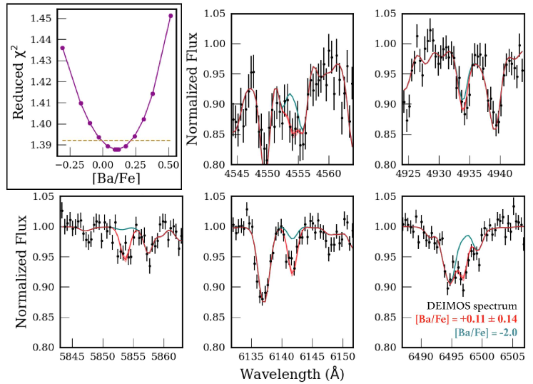
Figure 1: Example barium measurement for a single star in Draco. A DEIMOS medium-resolution spectrum (black) is shown alongside two synthetic spectra: the best-fit synthetic spectrum with the statistical error ranged shaded ($\text{[Ba/Fe]}=+0.11\pm 0.14$ dex, red) and one with $\text{[Ba/Fe]}=-2.0$ dex (blue). The top left panel shows the quality of the fit by comparing the reduced $\chi^{2}$ for synthetic spectra at a range of [Ba/Fe] values (purple). The horizontal dotted brown line indicates the one sigma uncertainty of the measurement. While most individual absorption lines are not highly significant, the simultaneous fit of five barium lines enables uncertainties of $\approx 0.2$ dex.

3.3 The Catalog

After we measured all the member stars in our sample, our catalog contains barium abundance measurements of 243 stars belonging to five dwarf galaxies, making this the largest self-consistent sample of dwarf galaxy barium abundances measured to date. Table 6 gives the multi-element abundance catalog for dwarf spheroidal galaxy (dSph) stars where [Ba/Fe] has been measured with uncertainties less than 0.28 dex. One advantage of this catalog of barium abundances is that this large sample of stars are all measured using the same assumptions in an automated way. This means that the catalog is internally consistent. The next section shows the consistency we achieve when comparing our [Ba/Fe] measurements to other measurements found in the literature, but it should be kept in mind that those literature measurements entail heterogeneous observations and measurement techniques.

Table 6: DEIMOS Multi-Element Abundances Catalog of dSph Stars

dSph	Name	RA	Dec	$T_{\rm{eff}}$	$\log g$	$\xi$	[Fe/H]	[$\alpha$/Fe]	[Ba/Fe]
				(K)	($g$ in cm s-2)	(km s-1)	(dex)	(dex)	(dex)
Dra	615574	17h20m07.44s	+57d54m32.7s	$4767\pm 46$	1.44	1.80	$-1.90\pm 0.10$	$-0.30\pm 0.18$	$+0.01\pm 0.24$
Dra	622253	17h19m57.29s	+57d55m04.6s	$4536\pm 23$	1.14	1.87	$-1.36\pm 0.10$	$-0.18\pm 0.09$	$+0.63\pm 0.13$
Dra	649595	17h20m01.59s	+57d57m04.6s	$4500\pm 34$	0.87	1.94	$-1.89\pm 0.10$	$-0.04\pm 0.10$	$+0.04\pm 0.16$
Dra	648189	17h19m57.91s	+57d56m58.4s	$4479\pm 27$	0.81	1.95	$-2.16\pm 0.10$	$+0.11\pm 0.09$	$-0.16\pm 0.16$
Dra	588559	17h20m13.51s	+57d51m59.3s	$4447\pm 23$	0.77	1.96	$-1.97\pm 0.10$	$+0.00\pm 0.09$	$-0.56\pm 0.15$
Dra	660453	17h20m05.66s	+57d57m52.8s	$4363\pm 24$	0.73	1.97	$-2.01\pm 0.10$	$+0.05\pm 0.09$	$+0.16\pm 0.15$
Dra	598482	17h20m16.12s	+57d52m56.1s	$4418\pm 49$	0.77	1.96	$-3.02\pm 0.10$	$+0.14\pm 0.18$	$-1.39\pm 0.24$
Dra	676918	17h20m03.97s	+57d59m08.3s	$4255\pm 16$	0.40	2.05	$-1.66\pm 0.10$	$-0.08\pm 0.09$	$+0.09\pm 0.13$
Dra	640120	17h20m05.78s	+57d56m23.4s	$4419\pm 27$	0.50	2.02	$-2.21\pm 0.10$	$+0.19\pm 0.09$	$-0.09\pm 0.13$
Dra	653393	17h19m58.88s	+57d57m20.9s	$4242\pm 20$	0.12	2.11	$-2.41\pm 0.10$	$+0.00\pm 0.09$	$-1.30\pm 0.14$

Note. — Table 6 is published in its entirety in the machine-readable format. A portion is shown here for guidance regarding its form and content. The errors reported here already include the systematic errors for [Fe/H], [$\alpha$/Fe], and [Ba/Fe] found in Table 11. Stars are only included if the errors for [Fe/H], [$\alpha$/Fe], and [Ba/Fe] are less than 0.28 dex.

4 Systematic Uncertainty

Beyond the [Ba/Fe] statistical errors returned by our fitting algorithm, we need to consider the systematic error of our measurement. The [Ba/Fe] statistical errors reflect the noise in the spectrum and how precisely the synthetic spectrum matches the observed spectrum. Technically, the statistical error reported is the square root of the diagonal values of the covariance matrix generated by Python’s scipy.optimize.curve_fit (Jones et al., 2001) function when fitting synthetic spectra to the observed spectrum. The [Ba/Fe] systematic error could be caused by the assumptions used in the spectral synthesis code (e.g., non-LTE effects), details of the method used to measure abundances, the line list, and how errors in other stellar parameters impact the [Ba/Fe] measured. The contribution of these sources help us to establish an error floor that is added in quadrature with the statistical errors to produce the errors reported in the catalog.

4.1 Appropriateness of the LTE Assumption

We use a spectral synthesis code that assumes local thermal equilibrium (LTE), because it greatly simplifies the computational burden. In the LTE case the opacity needs be known as a function of only temperature and density to solve for the flux. However, the impact of assuming LTE is perhaps the most significant assumption of all the assumptions made in the spectral synthesis code. Assuming LTE is valid only when the radiation field is closely coupled to the matter, which occurs through collisions between atoms and electrons. Therefore LTE holds at high densities.

A couple studies have carefully measured barium without assuming LTE (i.e., non-LTE) and compared them to LTE abundances published in the literature. For example, Andrievsky et al. (2009, 2017) found that the difference between [Ba/Fe] measured with and without assuming LTE varies from negligible to very significant ($\lesssim 0.8$ dex). The impact of assuming LTE on barium abundance measurements is primarily dependent on the $T_{\rm{eff}}$ and [Ba/H] of the star in question (Andrievsky et al., 2009). In addition, the details of the measurement (e.g., how many and which absorption lines are used) also plays a role on how sensitive the abundance measurements are to LTE effects.

To test the impact of assuming LTE with our observations, we measured a small, representative subset of stars with and without assuming LTE. We selected twelve stars that spanned the range of $T_{\rm{eff}}$ and [Ba/H] seen in our full sample. Both [Ba/Fe] measurements used the same DEIMOS spectra and stellar parameters. Andrievsky et al. (2017) describes the detailed methods of the non-LTE barium measurements. Our [Ba/Fe] measurements assuming LTE are consistent with the non-LTE measurements, as seen in Figure 2. The results are also reported in Table 7. Given that the impact of assuming LTE on [Ba/Fe] is well within the statistical uncertainties, no additional systematic uncertainty is needed to account for the effect of assuming LTE.

Table 7: Non-LTE Effects

dSph	Name	$T_{\rm{eff}}$	$\log g$	$\xi$	[Fe/H]	[$\alpha$/Fe]	[Ba/Fe]${}_{\text{LTE}}$	[Ba/Fe]${}_{\text{non-LTE}}$
		(K)	($g$ in cm s-2)	(km s-1)	(dex)	(dex)	(dex)	(dex)
For	74926	$3747\pm 11$	0.21	2.09	$-1.03\pm 0.10$	$-0.20\pm 0.10$	$+0.39\pm 0.19$	$+0.34$
For	64059	$3794\pm 12$	0.32	2.07	$-1.05\pm 0.10$	$-0.21\pm 0.10$	$+0.01\pm 0.19$	$+0.16$
For	58973	$3856\pm 11$	0.36	2.06	$-1.14\pm 0.10$	$-0.09\pm 0.10$	$+0.13\pm 0.17$	$+0.10$
For	55262	$4016\pm 19$	0.45	2.04	$-0.91\pm 0.10$	$+0.32\pm 0.13$	$+0.43\pm 0.17$	$+0.32$
Scl	1018551	$4182\pm 20$	0.53	2.02	$-1.72\pm 0.10$	$+0.14\pm 0.09$	$-0.05\pm 0.14$	$-0.05$
Scl	1008522	$4230\pm 14$	0.55	2.01	$-2.01\pm 0.10$	$+0.11\pm 0.09$	$+0.05\pm 0.13$	$+0.05$
Dra	653393	$4242\pm 20$	0.12	2.11	$-2.41\pm 0.10$	$+0.00\pm 0.09$	$-1.30\pm 0.14$	$-1.20$
Scl	1003537	$4280\pm 18$	0.58	2.01	$-2.26\pm 0.10$	$+0.21\pm 0.09$	$-0.32\pm 0.13$	$-0.33$
Scl	1013218	$4622\pm 44$	1.49	1.79	$-1.55\pm 0.10$	$-0.06\pm 0.11$	$+1.51\pm 0.11$	$+1.35$
Scl	1016539	$4614\pm 51$	1.40	1.81	$-1.76\pm 0.11$	$+0.17\pm 0.13$	$+0.18\pm 0.19$	$+0.19$
Scl	1010313	$4770\pm 52$	1.61	1.76	$-2.78\pm 0.13$	$+0.47\pm 0.17$	$-0.43\pm 0.21$	$-0.35$
UMi	Pal119	$5075\pm 48$	2.00	1.67	$-1.83\pm 0.11$	$-0.36\pm 0.23$	$+0.75\pm 0.21$	$+0.74$

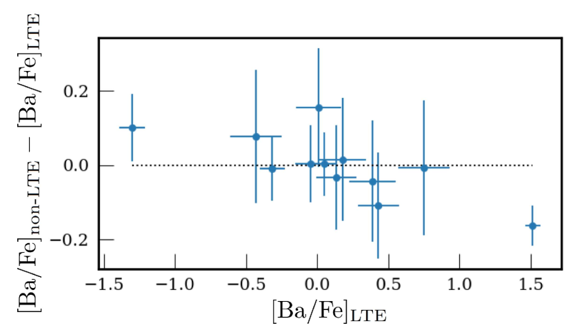
Figure 2: Comparison between our [Ba/Fe] measurements assuming LTE and without this assumption (i.e., non-LTE) using the same spectra and stellar parameters. These twelve representative stars show that the effect of assuming LTE is mostly within our statistical uncertainties.

4.2 Comparison to Other Catalogs

We must account for the systematic error introduced by any inaccuracies in the synthetic spectra and in the determination of stellar parameters. One way to account for this is to compare [Ba/Fe] measured for stars that overlap between our catalog and other catalogs published in the literature. All abundances have been shifted to the same solar abundance scale, which is described in Table 3. Table 8 highlights the different methods used by each literature source. Some of the differences between the measurements reflect the diversity of measurement techniques. In the following we refer to the literature sources as HRS because they all utilize high-resolution spectra. An advantage of our MRS sample is the uniformity of the acquisition and analysis of the spectra.

Table 8: Previously Published HRS Abundance Methods

Reference	System	Atmospheres	Code	$T_{\rm{eff}}$	$\log g$	$\xi$
Globular Clusters
Cohen & Kirby (2012)	NGC 2419	ATLAS9	MOOG	phot	phot	spec
Worley et al. (2013)	M15	ATLAS9	MOOG	phot	phot	spec
Lee et al. (2005)	M68	ATLAS9	MOOG	spec	spec	spec
Venn et al. (2012)	M68	MARCS	MOOG	spec	phot	spec
Halo Field Stars
Fulbright (2000)		ATLAS9	MOOG	spec	spec	spec
dSph
Aoki et al. (2007)	Ursa Minor	ATLAS9	Tsuji (1978), Aoki et al. (2009a)	spec	spec	spec
Cohen & Huang (2009, 2010)	Draco, Ursa Minor	ATLAS9	MOOG	spec	spec	spec
Geisler et al. (2005)	Sculptor	MARCS	MOOG	phot	spec	spec
Letarte, B. et al. (2018)	Fornax	MARCS	CALRAI	phot	phot	spec
Sadakane et al. (2004)	Ursa Minor	ATLAS9	SPTOOL	spec	spec	spec
Shetrone et al. (2001, 2003)	many	MARCS	MOOG	spec	spec	spec
Tsujimoto et al. (2017)	Draco	ATLAS9	Tsuji (1978), Aoki et al. (2009a)	phot	phot	spec

We compare a total of 57 stars that span [Ba/Fe] values from $-1.2$ to 0.8 dex. The stellar parameters and [Ba/Fe] measurements for both MRS and HRS methods are contained in Table 9. Figure 3 compares our barium abundances ([Ba/Fe]${}_{\text{MRS}}$) to the barium abundances published in the literature ([Ba/Fe]${}_{\text{HRS}}$). The barium abundances from MRS and HRS are largely consistent across the more than 1 dex span of [Ba/Fe] probed, but the difference ($\text{[Ba/Fe]}_{\text{MRS}}-\text{[Ba/Fe]}_{\text{HRS}}$) has a small average offset between the MRS and HRS [Ba/Fe] measurements of 0.03 dex. However, the difference ($\text{[Ba/Fe]}_{\text{MRS}}-\text{[Ba/Fe]}_{\text{HRS}}$) has a significant scatter.

Table 9: Comparison Between High-Resolution and DEIMOS Abundances

System	Name	HRS Reference	[Fe/H]${}_{\text{MRS}}$	[Ba/Fe]${}_{\text{MRS}}$	[Fe/H]${}_{\text{HRS}}$	[Ba/Fe]${}_{\text{HRS}}$
			(dex)	(dex)	(dex)	(dex)
NGC 2419	N2419-S1004	Cohen & Kirby (2012)	$-2.15\pm 0.09$	$-0.17\pm 0.22$	$-2.15\pm 0.14$	$-0.10\pm 0.19$
NGC 2419	N2419-S1065	Cohen & Kirby (2012)	$-2.11\pm 0.09$	$-0.01\pm 0.19$	$-2.10\pm 0.15$	$-0.21\pm 0.09$
NGC 2419	N2419-S1131	Cohen & Kirby (2012)	$-2.12\pm 0.08$	$+0.09\pm 0.17$	$-2.10\pm 0.15$	$+0.03\pm 0.05$
NGC 2419	N2419-S1166	Cohen & Kirby (2012)	$-2.04\pm 0.08$	$-0.29\pm 0.17$	$-2.07\pm 0.13$	$-0.18\pm 0.10$
NGC 2419	N2419-S1209	Cohen & Kirby (2012)	$-2.29\pm 0.08$	$-0.04\pm 0.17$	$-2.32\pm 0.11$	$+0.02\pm 0.16$
NGC 2419	N2419-S1305	Cohen & Kirby (2012)	$-2.21\pm 0.09$	$+0.03\pm 0.17$	$-2.25\pm 0.18$	$+0.19\pm 0.06$
NGC 2419	N2419-S1814	Cohen & Kirby (2012)	$-2.20\pm 0.08$	$+0.16\pm 0.15$	$-2.26\pm 0.14$	$-0.01\pm 0.18$
NGC 2419	N2419-S223	Cohen & Kirby (2012)	$-2.23\pm 0.08$	$+0.23\pm 0.16$	$-2.19\pm 0.15$	$+0.23\pm 0.24$
NGC 2419	N2419-S406	Cohen & Kirby (2012)	$-2.10\pm 0.09$	$+0.06\pm 0.17$	$-2.10\pm 0.13$	$-0.21\pm 0.10$
NGC 2419	N2419-S458	Cohen & Kirby (2012)	$-2.10\pm 0.09$	$+0.51\pm 0.17$	$-2.15\pm 0.15$	$-0.17\pm 0.17$

Note. — Table 9 is published in its entirety in the machine-readable format. Some columns (e.g., $T_{\rm{eff}}$, $\log g$, $\xi$ and [$\alpha$/Fe] for both MRS and HRS) are suppressed in the printed edition, and only the first ten lines are shown. Although the Milky Way halo field stars (Fulbright, 2000) were measured with the same stellar parameters (e.g., $T_{\rm{eff}}$, $\log g$, [Fe/H], [$\alpha$/Fe]) in both methods, stars in the dwarf galaxies and globular clusters have different stellar parameters in each method. Stars are only included if the errors for [Fe/H], [$\alpha$/Fe], and [Ba/Fe] are less than 0.28 dex.

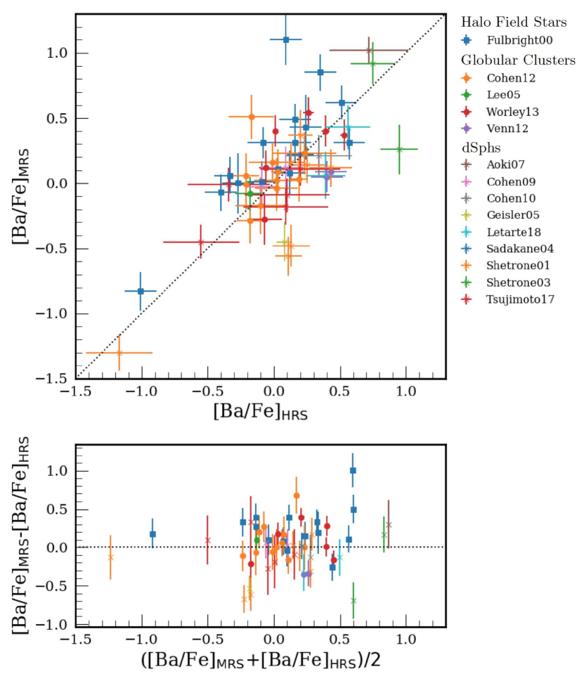
Figure 3: Comparison of our medium-resolution spectroscopy (MRS) to high-resolution spectroscopy (HRS) abundance measurements for 57 stars. See the legend of this figure or Table 9 for the sources of the HRS measurements.

The standard deviation of the offset between the MRS and HRS [Ba/Fe] measurements provides a metric to determine the systematic uncertainty. Assuming the uncertainties published in the HRS [Ba/Fe] measurements are prefect representations of the true error, we solved for the systematic uncertainty required to standardize the offset. This is done by solving Equation 2 for the systematic error ($\sigma_{\text{sys}}$).

$$\text{stddev}\left(\frac{\text{[Ba/Fe]}_{\text{MRS}}-\text{[Ba/Fe]}_{\text{HRS}}}{\sqrt{\sigma_{\text{HRS}}^{2}+\sigma_{\text{MRS}}^{2}+\sigma_{\text{sys}}^{2}}}\right)=1$$ (2)

Thus, $\sigma_{\text{sys}}$ is the error required to be added in quadrature with the MRS statistical error to force the dispersion between MRS and HRS to be unity. By comparing the MRS and HRS measurements of 57 stars, we measure $\sigma_{\text{sys}}=0.23$ dex. The resulting error distribution is shown in Figure 4.

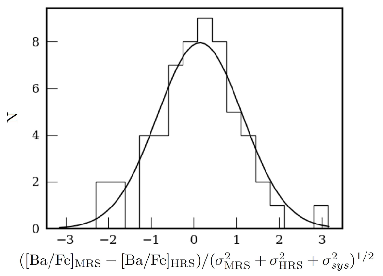
Figure 4: Distribution of differences between our medium-resolution spectroscopy (MRS) and high-resolution spectroscopy (HRS) measurements of [Ba/Fe] divided by the estimated error of the difference. The histogram contains 57 stars with a measured $\sigma_{\text{sys}}=0.23$. The curve is a Gaussian with $\sigma=1$.

4.3 Intrinsic Dispersion

With some exceptions (e.g., M15; Sneden et al., 1997), most globular clusters are expected to have no internal variation in heavy elements. Here we measure the systematic error that would be required to ensure there is no intrinsic dispersion of [Ba/Fe] in a globular cluster. This measurement was done with NGC 2419, M68, and M92 using Equation 3, where $\langle\text{[Ba/Fe]}\rangle$ is the average abundance. This assumes that these globular clusters do not have intrinsic dispersion in [Ba/Fe], which may or may not be the case (e.g., Roederer & Sneden, 2011; Cohen, 2011), so the systematic uncertainty returned is an upper limit. By standardizing the offset (see Equation 3) of the $\approx 30$ stars for which we were able to measure [Ba/Fe] in each globular cluster, we measure a $\sigma_{\text{sys}}=0.11$, 0.07, and 0.09 dex for NGC 2419, M68, and M92, respectively. The abundances can be seen in Figure 5, and they are included in Table 10. The error distribution when including the measured systematic errors are shown in Figure 6.

$$\text{stddev}\left(\frac{\text{[Ba/Fe]}-\langle\text{[Ba/Fe]}\rangle}{\sqrt{\sigma_{\text{stat}}^{2}+\sigma_{\text{sys}}^{2}}}\right)=1$$ (3)

Table 10: DEIMOS Multi-Element Abundances Catalog of Globular Cluster Stars

dSph	Name	RA	Dec	$T_{\rm{eff}}$	$\log g$	$\xi$	[Fe/H]	[$\alpha$/Fe]	[Ba/Fe]
				(K)	($g$ in cm s-2)	(km s-1)	(dex)	(dex)	(dex)
M92	Stet-M92-S1081	17h16m59.472	+43d07m09.58	$4971\pm 23$	2.06	1.66	$-2.45\pm 0.10$	$+0.31\pm 0.09$	$+0.03\pm 0.17$
M92	Stet-M92-S1377	17h17m02.346	+43d06m56.47	$5429\pm 34$	3.25	1.37	$-2.35\pm 0.11$	$+0.23\pm 0.12$	$-0.33\pm 0.16$
M92	Stet-M92-S1416	17h17m03.069	+43d06m36.66	$4983\pm 20$	2.06	1.65	$-2.37\pm 0.10$	$+0.25\pm 0.09$	$-0.11\pm 0.15$
M92	Stet-M92-S1622	17h17m02.321	+43d09m31.88	$4781\pm 30$	1.69	1.74	$-2.35\pm 0.10$	$+0.24\pm 0.09$	$-0.16\pm 0.14$
M92	Stet-M92-S1687	17h17m04.879	+43d07m32.34	$5431\pm 25$	2.92	1.45	$-2.27\pm 0.10$	$+0.33\pm 0.10$	$-0.30\pm 0.18$
M92	Stet-M92-S2476	17h17m07.992	+43d11m26.82	$5162\pm 26$	2.48	1.56	$-2.49\pm 0.10$	$+0.36\pm 0.09$	$-0.17\pm 0.12$
M92	Stet-M92-S2492	17h17m11.893	+43d07m28.93	$5721\pm 29$	3.52	1.31	$-2.19\pm 0.11$	$+0.22\pm 0.12$	$-0.16\pm 0.18$
M92	Stet-M92-S2732	17h17m11.044	+43d10m34.69	$5428\pm 27$	3.33	1.35	$-2.33\pm 0.11$	$+0.04\pm 0.13$	$-0.30\pm 0.15$
M92	Stet-M92-S2736	17h17m11.200	+43d10m28.52	$5053\pm 23$	2.15	1.63	$-2.47\pm 0.10$	$+0.31\pm 0.09$	$+0.20\pm 0.13$
M92	Stet-M92-S2977	17h17m12.782	+43d11m18.59	$5495\pm 29$	3.36	1.35	$-2.27\pm 0.11$	$+0.27\pm 0.12$	$-0.09\pm 0.17$

Note. — Table 10 is published in its entirety in the machine-readable format. A portion is shown here for guidance regarding its form and content. The errors reported here already include the systematic errors for [Fe/H], [$\alpha$/Fe], and [Ba/Fe] found in Table 11. Stars are only included if the errors for [Fe/H], [$\alpha$/Fe], and [Ba/Fe] are less than 0.28 dex.

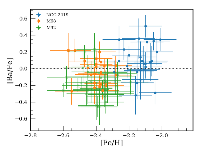
Figure 5: We have measured [Ba/Fe] for 26, 23, and 34 stars in NGC 2419, M68, and M92, respectively. This sample is used to constrain the systematic uncertainty of our measurement.

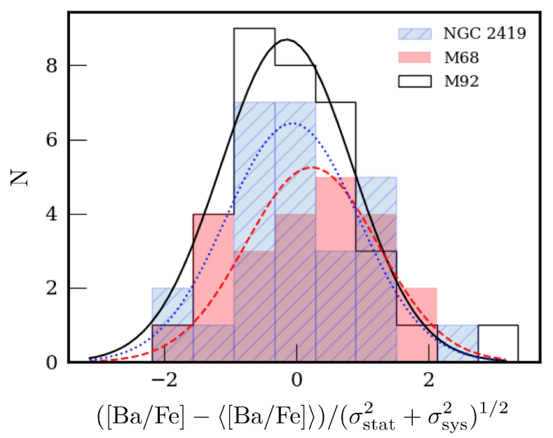
Figure 6: Distribution of differences from the average [Ba/Fe] measured in each globular cluster divided by the estimated error of the difference. By setting the intrinsic dispersion of NGC 2419, M68, and M92 to zero, we measured $\sigma_{\text{sys}}=0.11$, 0.07, and 0.09, respectively. The curves are Gaussians with $\sigma=1$.

4.4 Barium Abundance Error Floor

By comparing our [Ba/Fe] measurements to HRS measurements in the literature, we measure $\sigma_{sys}=0.23$. By forcing the [Ba/Fe] measurements of $\approx 30$ stars in NGC 2419, M68, and M92 to have no intrinsic dispersion, we measure $\sigma_{sys}=0.11$, 0.07, and 0.09, respectively. There is a clear discrepancy between the systematic error measured from the HRS comparison and the globular clusters. The HRS comparison relies on a heterogeneous collection of literature sources, with different spectrographs, line lists, and analysis codes. Some or most of the systematic error determined from HRS comes from this heterogeneity. On the other hand, the globular cluster analysis is internal to our own homogeneous study. Therefore, we set our systematic error at 0.1 dex for [Ba/Fe]. For context, the statistical errors of our measurements range from 0.1 to 0.28 dex with an average of 0.19 dex. All of the abundance error floors used in our catalog can be seen in Table 11.

Table 11: Abundance Error Floor

Abundance	Error Floor
[Fe/H]	0.101
[$\alpha$/Fe]	0.084
[Ba/Fe]	0.100

Note. — These systematic errors are included in the errors given in Table 6.

5 Discussion

We can observe neutron-capture abundance trends for several galaxies for the first time, because we have the largest sample of barium abundance measurements in dwarf galaxies ever assembled. We measured barium abundances in $\approx$250 stars with more than 30 red giant branch stars in each of Draco, Sculptor, Fornax, and Ursa Minor, in addition to five stars in Sextans (Figure 7). This catalog of abundances increases the number of stars with barium measurements in these galaxies substantially, which can be seen by comparing the number of stars with published [Ba/Fe] currently found in the literature ($N_{\text{LIT}}$) with the number of stars in our catalog ($N$) given in Table 12.

Table 12: Properties of Dwarf Galaxies

Galaxy	$D$	$M_{\ast}$	$\langle\tau_{\text{SF}}\rangle$	$\tau_{90}$	[Ba/Eu]${}_{\text{med}}$	$f_{r}$	$\langle$[Fe/H]$\rangle$	N	$\langle$[Ba/Fe]$\rangle$	N${}_{\text{LIT}}$
	(kpc)	($10^{5}$ M⊙)	(Gyr)	(Gyr)	(dex)	(%)	(dex)		(dex)
Fornax	$147\pm 9$	$190\pm 50$	7.4	2.3	$-0.19$	33%	$-0.99\pm 0.01$	30	$0.50\pm 0.03$	106
Sculptor	$85\pm 4$	$12\pm 5$	12.6	10.8	$-0.27$	40%	$-1.68\pm 0.01$	119	$-0.02\pm 0.02$	16
Draco	$75\pm 5$	$9.1\pm 1.4$	10.9	10.2	$-0.43$	58%	$-1.93\pm 0.01$	55	$0.04\pm 0.02$	24
Sextans	$85\pm 3$	$8.5\pm 2.4$	12.0	12.9	$\cdots$	$\cdots$	$-1.93\pm 0.01$	5	$-0.12\pm 0.08$	12
Ursa Minor	$75\pm 3$	$5.6\pm 1.7$	12.0	9.0	$-0.57$	80%	$-2.13\pm 0.01$	34	$0.33\pm 0.03$	20

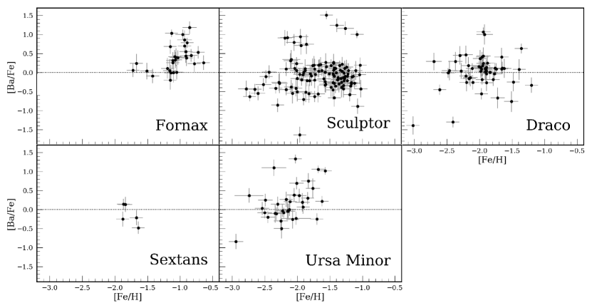
Figure 7: Barium abundance measurements in Fornax, Sculptor, Draco, Sextans, and Ursa Minor dwarf galaxies. This is the largest sample of barium measurements in dwarf galaxies ever assembled with a total of 243 stars. Our discussion focuses on the abundance trends seen for each galaxy. In this discussion, we neglect the high [Ba/Fe] outliers that are most clearly seen in Sculptor. These stars are likely to have been enriched by an AGB companion.

Before we discuss the abundance trends in these galaxies, it is important to discuss the very high [Ba/Fe] outliers that make up $\lesssim 10\%$ our sample. They are particularly obvious in Sculptor (10 stars with $\text{[Ba/Fe]}>0.5$), but likely contaminate the other dwarf galaxies as well. We believe that many of these barium-rich outliers are stars that have been in a binary with an AGB star at some point in their evolution. That AGB companion transferred $s$-process rich material onto the surface of the secondary star. The primary star since evolved into a white dwarf, leaving us to measure the polluted secondary red giant. Some literature studies have found similarly barium-rich stars ($\text{[Ba/Fe]}\approx 0.5$) and were able to use abundances of additional elements to confirm that they were enriched by an AGB companion (e.g., Honda et al., 2011). Additional elemental abundances would be required to prove that these outliers in our sample have been polluted by AGB stars, which is beyond the scope of this paper. If these stars have been polluted, they do not represent the chemical composition of the gas from which they were born and should therefore be ignored when discussing abundance trends. However, we leave these stars in our sample because we do not have confirmation (from light elements or radial velocity variations) that these stars were enriched by an AGB companion. The outliers are relatively rare, so they do not significantly bias our results.

5.1 Why AGB Stars are Not the Dominant Source of Barium Enrichment at Early Times

In Section 1.1 we isolated the potential large contributors of barium to AGB stars for the $s$-process, and either a rare type of CCSNe (e.g., MRSNe) or NSMs for the $r$-process. We now consider the $s$-process source of barium, AGB stars, and discuss why they are not expected to be the dominant source of barium at early times.

In the solar system, barium is primarily produced by the $s$-process (85%, Simmerer et al., 2004), which mainly occurs in AGB stars. However, each AGB star produces a small amount of barium ($\lesssim 10^{-6}$ M_⊙ of barium from AGB stars with $\text{[Fe/H]}\approx-0.7$; Karakas et al., 2018). In old, metal-poor stellar populations there has not been sufficient time for AGB stars to significantly contribute neutron-capture elements, and barium is instead an indicator of the $r$-process (e.g., Ji et al., 2016). Combining the knowledge currently available in the literature of the SFHs and [Ba/Eu] abundances for these dwarf galaxies confirms that AGB stars do not significantly contribute barium at early times ([Fe/H] $\lesssim-1.6$), and an $r$-process site is responsible for the majority of barium enrichment observed.

If the SFH is short, we will not see AGB stars contribute significantly because stars stopped forming before the bulk of the low-mass AGB stars evolved to the point of ejecting barium. Table 12 shows two independent tracers of the SFH: the average ages of the stars in the galaxies, $\langle\tau_{\text{SF}}\rangle$, and the time at which 90% of the stars in the galaxy have been formed, $\tau_{90}$. Both of these metrics confirm that although Fornax has had a comparably extended SFH, all of the other dwarf galaxies have short SFHs that could at most last 2–3 Gyrs. From the SFHs we would expect AGB stars to have the largest impact in Fornax because it has more extended star formation than the other dwarf galaxies. The contribution from AGB stars would only dominate the [Ba/Fe] trend in Sculptor, Ursa Minor, and Draco at late times (the iron-rich end), and therefore would not dominate barium production at low [Fe/H].

These conclusions are further confirmed by studying the [Ba/Eu] measurements found in the literature (see Figure 8). We convert these [Ba/Eu] ratios to the percentage of neutron-capture elements contributed by the $r$-process ($f_{r}$) using the pure $r$- and $s$-process abundances reported by Simmerer et al. (2004). Equation 4 describes this conversion. In this equation $N_{s/r}=10^{\log\epsilon_{s/r}}$, where $\log\epsilon_{s/r}$ is from Table 10 in Simmerer et al. (2004), and $f_{r}$ was restricted to remain between zero and one. The solar ratio $({\rm Ba/Eu})_{\odot}$ is given by Table 3.

$$f_{r}(\text{[Ba/Eu]})=\displaystyle\frac{\frac{N_{\text{Eu}-s}}{N_{\text{Ba}-s}}-10^{-(\text{[Ba/Eu]}+\text{(Ba/Eu)}_{\odot})}}{\frac{N_{\text{Eu}-s}}{N_{\text{Ba}-s}}-\frac{N_{\text{Eu}-r}}{N_{\text{Ba}-r}}}$$ (4)

The median $r$-process contribution in each galaxy is included in Table 12. The lowest $r$-process (i.e., the highest $s$-process) contributions occur in galaxies with the longest SFHs. Although we do see $s$-process (AGB) contribution dominate the barium contribution at higher [Fe/H] for Fornax and Sculptor, the [Ba/Eu] trends in most of these galaxies have [Ba/Eu] $\lesssim-0.4$ for [Fe/H] $\lesssim-1.6$. Sculptor is the exception to this statement (see Figure 8). However, extensive [Ba/Eu] measurements by Hill et al. (in prep) in Sculptor are lower than the measurements by Shetrone et al. (2003) and Geisler et al. (2005). The newer measurements do satisfy the criterion of [Ba/Eu] $\lesssim-0.4$ for [Fe/H] $\lesssim-1.6$ (these measurements are shown in Figure 14 of Tolstoy et al. 2009). A [Ba/Eu] value of $-0.4$ is equivalent to 54% of barium being contributed by the $r$-process. Therefore, AGB stars can not be the dominant source of barium at early times ([Fe/H] $\lesssim-1.6$).

5.2 Isolating the R-Process Contribution of Barium

Although AGB stars are not the dominant source of barium at early times, we still need to remove their contribution to clearly study the $r$-process. To isolate the barium contributed by the $r$-process exclusively, we utilize the [Ba/Eu] measurements found in the literature to subtract the $s$-process contribution. We first fit a line to the [Ba/Eu] and [Fe/H] measurements found in the literature (see Figure 8). This line can be converted (via Equation 4) to the fraction of barium coming from the $r$-process ($f_{r}$). We can now convert [Ba/Fe] from our catalog (Figure 7) and the literature to include only the $r$-process component by [Ba/Fe]${}_{r}=\text{[Ba/Fe]}+\log(f_{r})$. These results are displayed in the right panels of Figure 9. Now that we have isolated the $r$-process component of barium, we can discuss the $r$-process barium trend that we observe.

5.3 New Critical Piece of Evidence of the Dominant R-Process Origin

The key result of this paper is shown in Figure 9 where we compare [$\alpha$/Fe] (specifically [Mg/Fe], Kirby et al., 2010) as a function of [Fe/H] to the $r$-process component of [Ba/Fe] ([Ba/Fe]_r) as a function of [Fe/H]. Barium results from both this catalog (black circles) and the literature values (blue) are displayed to utilize all the available information. Linear fits to Kirby et al.’s and our catalog are shown in red with the slope of this fit printed for each galaxy. The trend is that [Mg/Fe] decreases with iron abundance because CCSNe contribute $\alpha$ elements before SNe Ia contribute large quantities of iron. However the barium abundances have slopes that are significantly more positive (even when accounting for the uncertainties of the slopes) for [Fe/H] $\lesssim-1.6$. This can be seen in Sculptor, Draco, and Ursa Minor. When possible, we allowed the slope to differ for [Fe/H] greater than and less than $-1.6$. There were only enough stars above and below this [Fe/H] cutoff in Sculptor to allow this broken slope. The [Fe/H] cutoff of $-1.6$ was chosen because visually the slope of [Ba/Fe] vs. [Fe/H] changes in Sculptor at approximately this [Fe/H] abundance.

The fact that all of the galaxies in our sample simultaneously have a negative [Mg/Fe] vs. [Fe/H] slope and a significantly more positive [Ba/Fe]_r vs. [Fe/H] slope for [Fe/H] $\lesssim-1.6$ leads to the conclusion that $r$-process barium is delayed relative to magnesium at early times. Therefore, Ba cannot come from the same source (CCSNe) as Mg.

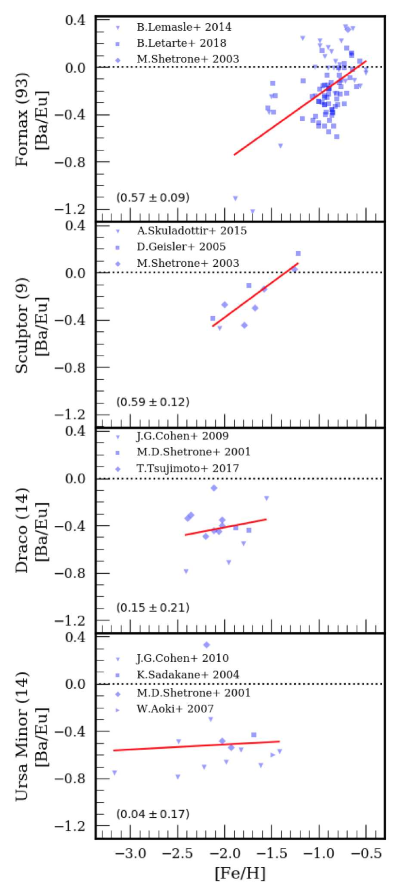
Figure 8: Literature [Ba/Eu] measurements for each galaxy. Additional [Ba/Eu] measurements for Sculptor by Hill et al. (in prep) show a lower [Ba/Eu] trend than shown in this plot (see Figure 14 of Tolstoy et al. 2009). Sextans is not included because no [Ba/Eu] detections exist. A line ($\text{[Ba/Eu]}=A\times\text{[Fe/H]}+B$) is fit to each galaxy’s abundances to determine the fraction of barium contributed via the $r$-process. The slope ($A$) of the line for each galaxy is printed on the bottom left.

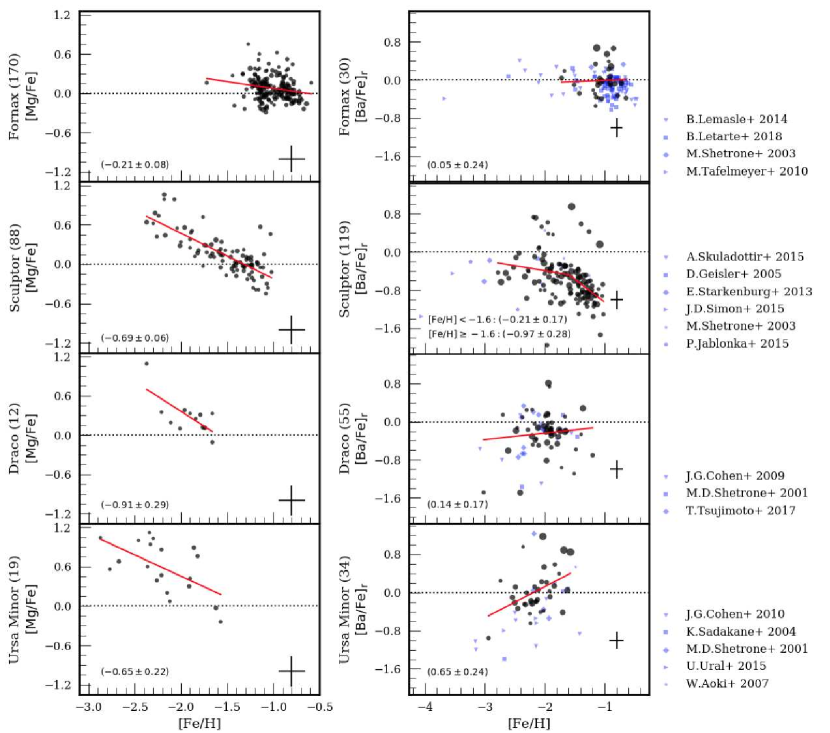
Figure 9: Comparison of the trend of [Mg/Fe] (Kirby et al., 2010) and [Ba/Fe] created by the $r$-process ([Ba/Fe]_r) as a function of [Fe/H] for each galaxy. The current published [Ba/Fe] abundances (adjusted to include only the $r$-process component) are shown in blue with the corresponding reference listed on the side. Overplotted in black are our [Ba/Fe]_r measurements. The sizes of the dots are inversely proportional to the errors, and the average errors for the stars plotted in each sub-figure are shown in the bottom right. The stars in black have abundance errors less than 0.28 dex and the total number plotted is listed in parentheses. A linear fit is shown in red, and the slope of this line is printed in the bottom left of each panel. The main conclusion is that [Mg/Fe] decreases as a function of [Fe/H] while [Ba/Fe] has a significantly more positive slope for low metallicities. This indicates that barium is contributed on a more delayed timescale than CCSNe.

The discrepant slopes of [Mg/Fe] and [Ba/Fe]_r vs. [Fe/H] are a powerful diagnostic feature of the $r$-process origin for a few different reasons. First, we are comparing consistent samples with the same techniques for these abundance measurements. Second, we are comparing abundance trends for the same galaxies. Therefore, both [Mg/Fe] and [Ba/Fe]_r are subject to the same SFH, gas inflow/outflow history, and [Fe/H] trend with time. This removes the dependence of our conclusion on a galactic chemical evolution model and its myriad assumptions. Third, we see the discrepant slopes in multiple dwarf galaxies. This proves that we are seeing a global characteristic of the $r$-process.

Our observation of a significantly more positive slope of [Ba/Fe]_r vs. [Fe/H] than [$\alpha$/Fe]for low iron abundances ([Fe/H] $\lesssim-1.6$) in several dwarf galaxies, requires that the timescale for barium is substantially more delayed than the timescale for magnesium. We now consider the possible origins for barium and which source would cause the observed trends.

5.4 NSMs Could Be the Dominant Source of Barium in Dwarf Galaxies

We have concluded that dwarf galaxies are dominated by a $r$-process source with a timescale more delayed than CCSNe at early times ([Fe/H] $\lesssim-1.6$). Compared to ultra-faint dwarfs (Ji et al., 2016; Hansen et al., 2017), our sample of classical dwarf galaxies is able to probe the characteristics of an ensemble of $r$-process enrichment rather than isolated events. This evidence includes information about the timescale of enrichment, which enables us to distinguish whether MRSNe or NSMs are the dominant source of $r$-process enrichment in dwarf galaxies at early times.

First we will consider MRSNe. All CCSNe have a short lifetime, so they would cause the same negative trend that we see in the $\alpha$ elements, which are also released by CCSNe. Even if the $r$-process arises from very rare types of CCSN, like MRSNe, we would expect an overall negative—and perhaps jagged—slope in [$r$/Fe] vs. [Fe/H]. Because we observe a significantly more positive [Ba/Fe]_r vs. [Fe/H] slope, we can rule out MRSNe as the dominant source of barium in these dwarf galaxies. Common envelope jets SNe have a slightly longer delay time than CCSNe, but the delay time is still set by the lifetime of the secondary star in the binary system. Because both stars in this scenario are massive, their delay times would be much closer to CCSNe than NSMs, whose delay times are set by their protracted orbital decay.

Instead, we need a delayed barium enrichment to create a more positive [Ba/Fe]_r vs. [Fe/H] slope when compared to the [Mg/Fe] vs. [Fe/H] slope. A flat [Ba/Fe]_r vs. [Fe/H] trend would indicate that the $r$-process enrichment needs to occur on a timescale similar to SNe Ia because barium would need to be ejected into the ISM while SNe Ia are ejecting large amounts of iron. Although we see a clear increasing [Ba/Fe]_r vs. [Fe/H] trend in Ursa Minor and a flat or slightly rising trend in Draco, Sculptor has a slightly negative trend for $\text{[Fe/H]}\lesssim-1.6$. It is therefore ambiguous when the $r$-process enrichment needs to occur compared to SNe Ia timescales. However, we can definitively say that the timescale needs to be delayed compared to CCSNe in order to create the significantly more positive [Ba/Fe]_r vs. [Fe/H] slope. Based on our observations, NSMs are the most viable source of barium enrichment in dwarf galaxies at early times. Simulations and the LIGO observation support NSMs producing $r$-process elements (e.g., Goriely et al., 2011; Abbott et al., 2017; Côté et al., 2017).

In conclusion, our observations are matched by a source that releases barium on a timescale more delayed than CCSNe at early times. Of the sources suggested so far, neutron star mergers are the only source that satisfies this condition.

5.5 Implications

The early chemical evolution of dwarf galaxies can be used to constrain the yield and/or rate of NSMs, which we will address with a galactic chemical evolution model in a future paper. We have concluded that $r$-process enrichment is dominated by NSMs in the early evolution of dwarf galaxies. It is tempting to extrapolate this conclusion and apply this directly to comment on the dominant site of $r$-process enrichment in later evolution of dwarf galaxies and larger galaxies (such as the Milky Way).

However, we exhort readers to extrapolate to high [Fe/H] with caution. The rate of NSMs that have ejected material retained in the galaxy (and the yield or amount of ejected material that is retained per NSM) may depend on the age of the binary neutron star system and/or mass of the galaxy. To discuss the $r$-process trends seen in the literature at higher iron abundances, we turn to [Eu/Fe] as an indicator of the $r$-process, because the $s$-process is increasingly important in barium productions at these times. For example, Hill et al. (in prep) find a declining [Eu/Fe] vs. [Fe/H] trend (see Figure 13 in Tolstoy et al. 2009) in Sculptor at $\text{[Fe/H]}\gtrsim-1.6$. Comparisons to the Milky Way are more challenging due to the drastically different mass and merger history. Milky Way halo stars are largely a compilation of stars stripped from dwarf galaxies. It is therefore unsurprising that there is a large spread in [Eu/Fe]. In Milky Way disk stars ([Fe/H] $\gtrsim-1.0$) a declining [Eu/Fe] vs. [Fe/H] trend is also observed (Battistini & Bensby, 2016). The complexity of the Milky Way relative to dwarf galaxies has led to varying conclusions as to whether the origin of the $r$-process is NSMs, MRSNe, or both (e.g., Cescutti et al., 2015; Wehmeyer et al., 2015).

This transition from positive [$r$-process/Fe] vs. [Fe/H] trends at low metallicities to a declining trend at higher metallicities presents a puzzle. Although some attribute this to MRSNe (Tsujimoto & Nishimura, 2015), another possible explanation is that NSM natal kicks cause the effective NSM rate (rate of NSMs contributing enriched material to the ISM) to decrease significantly at later times as the NSMs occur far from the galaxy (e.g., Willems & Kalogera, 2004; Bramante & Linden, 2016; Beniamini et al., 2016a; Safarzadeh & Scannapieco, 2017). It is important to note that the velocities of these NSM natal kicks are still unknown, and it is possible that they are large enough to remove the neutron star binary from the galaxy before a NSM can occur. Moderate NSM natal kicks that allow early NSMs to occur in the galaxy and late NSMs occur outside the galaxy would be consistent with our [Ba/Fe]_r measurements, specifically the significant decrease in [Ba/Fe]_r vs. [Fe/H] slope seen in Sculptor above and below $\text{[Fe/H]}=-1.6$). Additional detections of [Eu/Fe] with [Fe/H] $\lesssim-1.6$ and modeling of NSM natal kicks would be able to confirm the plausibility of this explanation.

6 Summary

Here we highlight the main conclusions of this paper.

• We have confirmed medium-resolution spectroscopy as a reliable method of measuring barium.

• We have obtained the largest sample of barium abundances in dwarf galaxies.

• We have discovered that the majority of barium in dwarf galaxies is created by a delayed $r$-process source at early times.

• We conclude that neutron star mergers are the most likely source of barium enrichment in dwarf galaxies at early times.

In a subsequent paper we will use galactic chemical evolution models to derive qualitative conclusions concerning the sources of barium enrichment in dwarf galaxies. Specifically, we will constrain the NSM yields/rates needed to match our observations.

References

- Abbott et al. (2017) Abbott, B. P., Abbott, R., Abbott, T. D., et al. 2017, Physical Review Letters, 119, 161101
- Anders & Grevesse (1989) Anders, E., & Grevesse, N. 1989, Geochim. Cosmochim. Acta, 53, 197
- Andrievsky et al. (2017) Andrievsky, S. M., Korotin, S. A., Hill, V., & Zhukova, A. V. 2017, arXiv:1710.04930
- Andrievsky et al. (2009) Andrievsky, S. M., Spite, M., Korotin, S. A., et al. 2009, A&A, 494, 1083
- Aoki et al. (2009a) Aoki, W., Barklem, P. S., Beers, T. C., et al. 2009a, ApJ, 698, 1803
- Aoki et al. (2007) Aoki, W., Honda, S., Sadakane, K., & Arimoto, N. 2007, PASJ, 59, L15
- Aoki et al. (2009b) Aoki, W., Arimoto, N., Sadakane, K., et al. 2009b, A&A, 502, 569
- Arnould et al. (2007) Arnould, M., Goriely, S., & Takahashi, K. 2007, Phys. Rep., 450, 97
- Barack et al. (2018) Barack, L., Cardoso, V., Nissanke, S., et al. 2018, ArXiv e-prints, arXiv:1806.05195
- Battistini & Bensby (2016) Battistini, C., & Bensby, T. 2016, A&A, 586, A49
- Bellazzini et al. (2002) Bellazzini, M., Ferraro, F. R., Origlia, L., et al. 2002, AJ, 124, 3222
- Beniamini et al. (2018) Beniamini, P., Dvorkin, I., & Silk, J. 2018, MNRAS, 478, 1994
- Beniamini et al. (2016a) Beniamini, P., Hotokezaka, K., & Piran, T. 2016a, ApJ, 829, L13
- Beniamini et al. (2016b) —. 2016b, ApJ, 832, 149
- Bensby et al. (2014) Bensby, T., Feltzing, S., & Oey, M. S. 2014, A&A, 562, A71
- Bettinelli et al. (2018) Bettinelli, M., Hidalgo, S. L., Cassisi, S., Aparicio, A., & Piotto, G. 2018, MNRAS, 476, 71
- Bramante & Linden (2016) Bramante, J., & Linden, T. 2016, ApJ, 826, 57
- Castelli & Kurucz (2004) Castelli, F., & Kurucz, R. L. 2004, ArXiv Astrophysics e-prints, astro-ph/0405087
- Cescutti et al. (2015) Cescutti, G., Romano, D., Matteucci, F., Chiappini, C., & Hirschi, R. 2015, A&A, 577, A139
- Cohen (2011) Cohen, J. G. 2011, ApJ, 740, L38
- Cohen & Huang (2009) Cohen, J. G., & Huang, W. 2009, ApJ, 701, 1053
- Cohen & Huang (2010) —. 2010, ApJ, 719, 931
- Cohen & Kirby (2012) Cohen, J. G., & Kirby, E. N. 2012, ApJ, 760, 86
- Cooper et al. (2012) Cooper, M. C., Newman, J. A., Davis, M., Finkbeiner, D. P., & Gerke, B. F. 2012, spec2d: DEEP2 DEIMOS Spectral Pipeline, Astrophysics Source Code Library, , , ascl:1203.003
- Côté et al. (2017) Côté, B., Belczynski, K., Fryer, C. L., et al. 2017, ApJ, 836, 230
- Coulter et al. (2017) Coulter, D. A., Foley, R. J., Kilpatrick, C. D., et al. 2017, Science, 358, 1556
- De Cia et al. (2018) De Cia, A., Gal-Yam, A., Rubin, A., et al. 2018, ApJ, 860, 100
- Escala et al. (2018) Escala, I., Wetzel, A., Kirby, E. N., et al. 2018, MNRAS, 474, 2194
- Evans et al. (2017) Evans, P. A., Cenko, S. B., Kennea, J. A., et al. 2017, Science, 358, 1565
- Faber et al. (2003) Faber, S. M., Phillips, A. C., Kibrick, R. I., et al. 2003, in Proc. SPIE, Vol. 4841, Instrument Design and Performance for Optical/Infrared Ground-based Telescopes, ed. M. Iye & A. F. M. Moorwood, 1657–1669
- Foucart et al. (2015) Foucart, F., O’Connor, E., Roberts, L., et al. 2015, Phys. Rev. D, 91, 124021
- Fulbright (2000) Fulbright, J. P. 2000, AJ, 120, 1841
- Fulbright (2002) —. 2002, AJ, 123, 404
- Geisler et al. (2005) Geisler, D., Smith, V. V., Wallerstein, G., Gonzalez, G., & Charbonnel, C. 2005, AJ, 129, 1428
- Gilmore & Wyse (1991) Gilmore, G., & Wyse, R. F. G. 1991, ApJ, 367, L55
- Goriely et al. (2011) Goriely, S., Bauswein, A., & Janka, H.-T. 2011, ApJ, 738, L32
- Grichener & Soker (2018) Grichener, A., & Soker, N. 2018, ArXiv e-prints, arXiv:1810.03889
- Gustafsson et al. (1975) Gustafsson, B., Bell, R. A., Eriksson, K., & Nordlund, A. 1975, A&A, 42, 407
- Gustafsson et al. (2008) Gustafsson, B., Edvardsson, B., Eriksson, K., et al. 2008, A&A, 486, 951
- Gustafsson et al. (2003) Gustafsson, B., Edvardsson, B., Eriksson, K., et al. 2003, in Astronomical Society of the Pacific Conference Series, Vol. 288, Stellar Atmosphere Modeling, ed. I. Hubeny, D. Mihalas, & K. Werner, 331
- Hansen et al. (2017) Hansen, T. T., Simon, J. D., Marshall, J. L., et al. 2017, ApJ, 838, 44
- Harris (1996) Harris, W. E. 1996, AJ, 112, 1487
- Hinkle et al. (2000) Hinkle, K., Wallace, L., Valenti, J., & Harmer, D. 2000, Visible and Near Infrared Atlas of the Arcturus Spectrum 3727-9300 A
- Honda et al. (2011) Honda, S., Aoki, W., Arimoto, N., & Sadakane, K. 2011, PASJ, 63, 523
- Iwamoto et al. (1999) Iwamoto, K., Brachwitz, F., Nomoto, K., et al. 1999, ApJS, 125, 439
- Jablonka et al. (2015) Jablonka, P., North, P., Mashonkina, L., et al. 2015, A&A, 583, A67
- Ji & Frebel (2018) Ji, A. P., & Frebel, A. 2018, ApJ, 856, 138
- Ji et al. (2016) Ji, A. P., Frebel, A., Chiti, A., & Simon, J. D. 2016, Nature, 531, 610
- Jones et al. (2001) Jones, E., Oliphant, T., Peterson, P., et al. 2001, SciPy: Open source scientific tools for Python, , , [Online; accessed 2017-01-16]
- Karakas & Lattanzio (2014) Karakas, A. I., & Lattanzio, J. C. 2014, PASA, 31, e030
- Karakas et al. (2018) Karakas, A. I., Lugaro, M., Carlos, M., et al. 2018, MNRAS, 477, 421
- Kasen & Bildsten (2010) Kasen, D., & Bildsten, L. 2010, ApJ, 717, 245
- Kirby et al. (2014) Kirby, E. N., Bullock, J. S., Boylan-Kolchin, M., Kaplinghat, M., & Cohen, J. G. 2014, MNRAS, 439, 1015
- Kirby et al. (2011a) Kirby, E. N., Cohen, J. G., Smith, G. H., et al. 2011a, ApJ, 727, 79
- Kirby et al. (2009) Kirby, E. N., Guhathakurta, P., Bolte, M., Sneden, C., & Geha, M. C. 2009, ApJ, 705, 328
- Kirby et al. (2016) Kirby, E. N., Guhathakurta, P., Zhang, A. J., et al. 2016, ApJ, 819, 135
- Kirby et al. (2011b) Kirby, E. N., Lanfranchi, G. A., Simon, J. D., Cohen, J. G., & Guhathakurta, P. 2011b, ApJ, 727, 78
- Kirby et al. (2010) Kirby, E. N., Guhathakurta, P., Simon, J. D., et al. 2010, ApJS, 191, 352
- Kirby et al. (2015) Kirby, E. N., Guo, M., Zhang, A. J., et al. 2015, ApJ, 801, 125
- Kurucz (1993) Kurucz, R. 1993, ATLAS9 Stellar Atmosphere Programs and 2 km/s grid. Kurucz CD-ROM No. 13. Cambridge, Mass.: Smithsonian Astrophysical Observatory, 1993., 13
- Lattimer & Schramm (1974) Lattimer, J. M., & Schramm, D. N. 1974, ApJ, 192, L145
- Lee et al. (2005) Lee, J.-W., Carney, B. W., & Habgood, M. J. 2005, AJ, 129, 251
- Lee et al. (2003) Lee, M. G., Park, H. S., Park, J.-H., et al. 2003, AJ, 126, 2840
- Lemasle et al. (2014) Lemasle, B., de Boer, T. J. L., Hill, V., et al. 2014, A&A, 572, A88
- Letarte et al. (2010) Letarte, B., Hill, V., Tolstoy, E., et al. 2010, A&A, 523, A17
- Letarte, B. et al. (2018) Letarte, B., Hill, V., Tolstoy, E., et al. 2018, A&A, 613, C1
- Liccardo et al. (2018) Liccardo, V., Malheiro, M., Hussein, M. S., & Frederico, T. 2018, ArXiv e-prints, arXiv:1805.10183
- Macias & Ramirez-Ruiz (2016) Macias, P., & Ramirez-Ruiz, E. 2016, ArXiv e-prints, arXiv:1609.04826
- Maoz & Graur (2017) Maoz, D., & Graur, O. 2017, ApJ, 848, 25
- Mateo (1998) Mateo, M. L. 1998, ARA&A, 36, 435
- McWilliam (1998) McWilliam, A. 1998, AJ, 115, 1640
- Mighell & Burke (1999) Mighell, K. J., & Burke, C. J. 1999, AJ, 118, 366
- Mösta et al. (2017) Mösta, P., Roberts, L. F., Halevi, G., et al. 2017, ArXiv e-prints, arXiv:1712.09370
- Newman et al. (2013) Newman, J. A., Cooper, M. C., Davis, M., et al. 2013, ApJS, 208, 5
- Nishimura et al. (2017) Nishimura, N., Sawai, H., Takiwaki, T., Yamada, S., & Thielemann, F.-K. 2017, ApJ, 836, L21
- Nishimura et al. (2015) Nishimura, N., Takiwaki, T., & Thielemann, F.-K. 2015, ApJ, 810, 109
- Nomoto et al. (2006) Nomoto, K., Tominaga, N., Umeda, H., Kobayashi, C., & Maeda, K. 2006, Nuclear Physics A, 777, 424
- Orban et al. (2008) Orban, C., Gnedin, O. Y., Weisz, D. R., et al. 2008, ApJ, 686, 1030
- Papish et al. (2015) Papish, O., Soker, N., & Bukay, I. 2015, MNRAS, 449, 288
- Pietrzyński et al. (2008) Pietrzyński, G., Gieren, W., Szewczyk, O., et al. 2008, AJ, 135, 1993
- Radice et al. (2016) Radice, D., Galeazzi, F., Lippuner, J., et al. 2016, MNRAS, 460, 3255
- Ramírez & Allende Prieto (2011) Ramírez, I., & Allende Prieto, C. 2011, ApJ, 743, 135
- Rizzi et al. (2007) Rizzi, L., Held, E. V., Saviane, I., Tully, R. B., & Gullieuszik, M. 2007, MNRAS, 380, 1255
- Roederer & Sneden (2011) Roederer, I. U., & Sneden, C. 2011, AJ, 142, 22
- Ryabchikova et al. (2015) Ryabchikova, T., Piskunov, N., Kurucz, R. L., et al. 2015, Phys. Scr, 90, 054005
- Sadakane et al. (2004) Sadakane, K., Arimoto, N., Ikuta, C., et al. 2004, PASJ, 56, 1041
- Safarzadeh & Scannapieco (2017) Safarzadeh, M., & Scannapieco, E. 2017, MNRAS, 471, 2088
- Shetrone et al. (2003) Shetrone, M., Venn, K. A., Tolstoy, E., et al. 2003, AJ, 125, 684
- Shetrone et al. (2001) Shetrone, M. D., Côté, P., & Sargent, W. L. W. 2001, ApJ, 548, 592
- Shibata & Taniguchi (2011) Shibata, M., & Taniguchi, K. 2011, Living Reviews in Relativity, 14, 6
- Simmerer et al. (2004) Simmerer, J., Sneden, C., Cowan, J. J., et al. 2004, ApJ, 617, 1091
- Simon et al. (2015) Simon, J. D., Jacobson, H. R., Frebel, A., et al. 2015, ApJ, 802, 93
- Skúladóttir et al. (2015) Skúladóttir, Á., Tolstoy, E., Salvadori, S., et al. 2015, A&A, 574, A129
- Sneden et al. (2012) Sneden, C., Bean, J., Ivans, I., Lucatello, S., & Sobeck, J. 2012, MOOG: LTE line analysis and spectrum synthesis, Astrophysics Source Code Library, , , ascl:1202.009
- Sneden et al. (2008) Sneden, C., Cowan, J. J., & Gallino, R. 2008, ARA&A, 46, 241
- Sneden et al. (1992) Sneden, C., Kraft, R. P., Prosser, C. F., & Langer, G. E. 1992, AJ, 104, 2121
- Sneden et al. (1997) Sneden, C., Kraft, R. P., Shetrone, M. D., et al. 1997, AJ, 114, 1964
- Sneden et al. (2014) Sneden, C., Lucatello, S., Ram, R. S., Brooke, J. S. A., & Bernath, P. 2014, ApJS, 214, 26
- Sneden (1973) Sneden, C. A. 1973, PhD thesis, THE UNIVERSITY OF TEXAS AT AUSTIN.
- Soker & Gilkis (2017) Soker, N., & Gilkis, A. 2017, ApJ, 851, 95
- Spite (1967) Spite, M. 1967, Annales d’Astrophysique, 30, 211
- Starkenburg et al. (2013) Starkenburg, E., Hill, V., Tolstoy, E., et al. 2013, A&A, 549, A88
- Suda et al. (2017) Suda, T., Hidaka, J., Aoki, W., et al. 2017, PASJ, 69, 76
- Tafelmeyer et al. (2010) Tafelmeyer, M., Jablonka, P., Hill, V., et al. 2010, A&A, 524, A58
- Takeda (1995) Takeda, Y. 1995, PASJ, 47, 287
- Tanvir et al. (2017) Tanvir, N. R., Levan, A. J., González-Fernández, C., et al. 2017, ApJ, 848, L27
- Thielemann et al. (2011) Thielemann, F.-K., Arcones, A., Käppeli, R., et al. 2011, Progress in Particle and Nuclear Physics, 66, 346
- Tinsley (1980) Tinsley, B. M. 1980, Fund. Cosmic Phys., 5, 287
- Tolstoy et al. (2009) Tolstoy, E., Hill, V., & Tosi, M. 2009, ARA&A, 47, 371
- Tolstoy et al. (2006) Tolstoy, E., Hill, V., Irwin, M., et al. 2006, The Messenger, 123
- Troja et al. (2017) Troja, E., Piro, L., van Eerten, H., et al. 2017, Nature, 551, 71
- Tsuji (1978) Tsuji, T. 1978, A&A, 62, 29
- Tsujimoto et al. (2017) Tsujimoto, T., Matsuno, T., Aoki, W., Ishigaki, M. N., & Shigeyama, T. 2017, ApJ, 850, L12
- Tsujimoto & Nishimura (2015) Tsujimoto, T., & Nishimura, N. 2015, ApJ, 811, L10
- Ural et al. (2015) Ural, U., Cescutti, G., Koch, A., et al. 2015, MNRAS, 449, 761
- Venn et al. (2004) Venn, K. A., Irwin, M., Shetrone, M. D., et al. 2004, AJ, 128, 1177
- Venn et al. (2012) Venn, K. A., Shetrone, M. D., Irwin, M. J., et al. 2012, ApJ, 751, 102
- Wanajo (2013) Wanajo, S. 2013, ApJ, 770, L22
- Wehmeyer et al. (2015) Wehmeyer, B., Pignatari, M., & Thielemann, F.-K. 2015, MNRAS, 452, 1970
- Weisz et al. (2014) Weisz, D. R., Dolphin, A. E., Skillman, E. D., et al. 2014, ApJ, 789, 148
- Willems & Kalogera (2004) Willems, B., & Kalogera, V. 2004, ApJ, 603, L101
- Woo et al. (2008) Woo, J., Courteau, S., & Dekel, A. 2008, MNRAS, 390, 1453
- Woosley & Janka (2005) Woosley, S., & Janka, T. 2005, Nature Physics, 1, 147
- Worley et al. (2013) Worley, C. C., Hill, V., Sobeck, J., & Carretta, E. 2013, A&A, 553, A47