Motion Planning in Irreducible Path Spaces

Abstract

The motion of a mechanical system can be defined as a path through its configuration space. Computing such a path has a computational complexity scaling exponentially with the dimensionality of the configuration space. We propose to reduce the dimensionality of the configuration space by introducing the irreducible path — a path having a minimal swept volume. The paper consists of three parts: In part I, we define the space of all irreducible paths and show that planning a path in the irreducible path space preserves completeness of any motion planning algorithm. In part II, we construct an approximation to the irreducible path space of a serial kinematic chain under certain assumptions. In part III, we conduct motion planning using the irreducible path space for a mechanical snake in a turbine environment, for a mechanical octopus with eight arms in a pipe system and for the sideways motion of a humanoid robot moving through a room with doors and through a hole in a wall. We demonstrate that the concept of an irreducible path can be applied to any motion planning algorithm taking curvature constraints into account.

1

2 Introduction

Motion planning [1] has been succesfully applied to many mechanical systems with applications in computer graphics, humanoid robotics or protein folding. The key idea of motion planning is to define the motion of a mechanical system as a path through its configuration space. Given two configurations, the goal of motion planning is to construct a motion planning algorithm computing a path connecting the two configurations.

Real-world systems like mechanical snakes or humanoid robots have many degrees of freedom (DoF) and therefore a high-dimensional configuration space. The higher the dimensionality of the configuration space, the more time a motion planning algorithm needs to find a solution. In fact, any motion planning algorithm has a computational complexity scaling exponentially with the dimensionality of the configuration space [2].

A key challenge in motion planning is therefore to reduce the dimensionality of the configuration space. Dimensionality reduction of configuration spaces has been addressed by several researchers [3, 4, 5], but the results only apply in special cases. In fact, there is no general approach to reduce the dimensionality of a configuration space in a principled way.

Our work contributes to this effort by introducing the irreducible path [6], a configuration space path having a minimal swept volume . The space of all those minimal swept volume paths creates the irreducible path space. Our main result is Theorem 3, which shows that replacing the full space of continuous paths with the space of irreducible paths preserves completeness of any motion planning algorithm. This is advantageous because computing an irreducible path can often be done in a lower dimensional configuration space, thereby reducing the computational complexity.

The paper consists of three parts. In Part I we define the irreducible path and the irreducible path space. We discuss the partitioning of the irreducible path space under equivalent swept volumes. We then prove the completeness of any motion planning algorithm using the irreducible path space in Theorem 3. We note that those concepts apply to any functional space: the space of all dynamical feasible paths, all statically stable paths, all torque constraint paths or all collision-free paths. For sake of simplicity, we focus here exclusively on collision-free paths.

In Part II, we approximate the irreducible path space of a serial kinematic chain. The main idea is the following: if the root link moves on a curvature-constraint path, then all the sublinks can be projected into the swept volume of the root link. Therefore, we can ignore the sublinks and we can thereby reduce the dimensionality of the configuration space. This has been visualized in the case of a serial kinematic chain in the plane in Fig. 1.

In Part III, we apply the reduction of the serial kinematic chain to four different mechanical systems: an idealized serial kinematic chain on $SE(2)\times\mathbb{R}^{3}$, $SE(2)\times\mathbb{R}^{6}$ and $SE(3)\times\mathbb{R}^{12}$, a mechanical snake in a turbine environment on $SE(3)\times\mathbb{R}^{16}$, a mechanical octopus in a tunnel system on $SE(3)\times\mathbb{R}^{80}$ and a humanoid robot moving sideways on $SE(2)\times\mathbb{R}^{19}$ through a room with doors and through a hole in a wall.

This work extends previous results in [6], where we introduced the irreducible path and applied it to the sideway motion of a humanoid robot. Section 4 is based on [6], it has been revised and the proofs have been simplified.

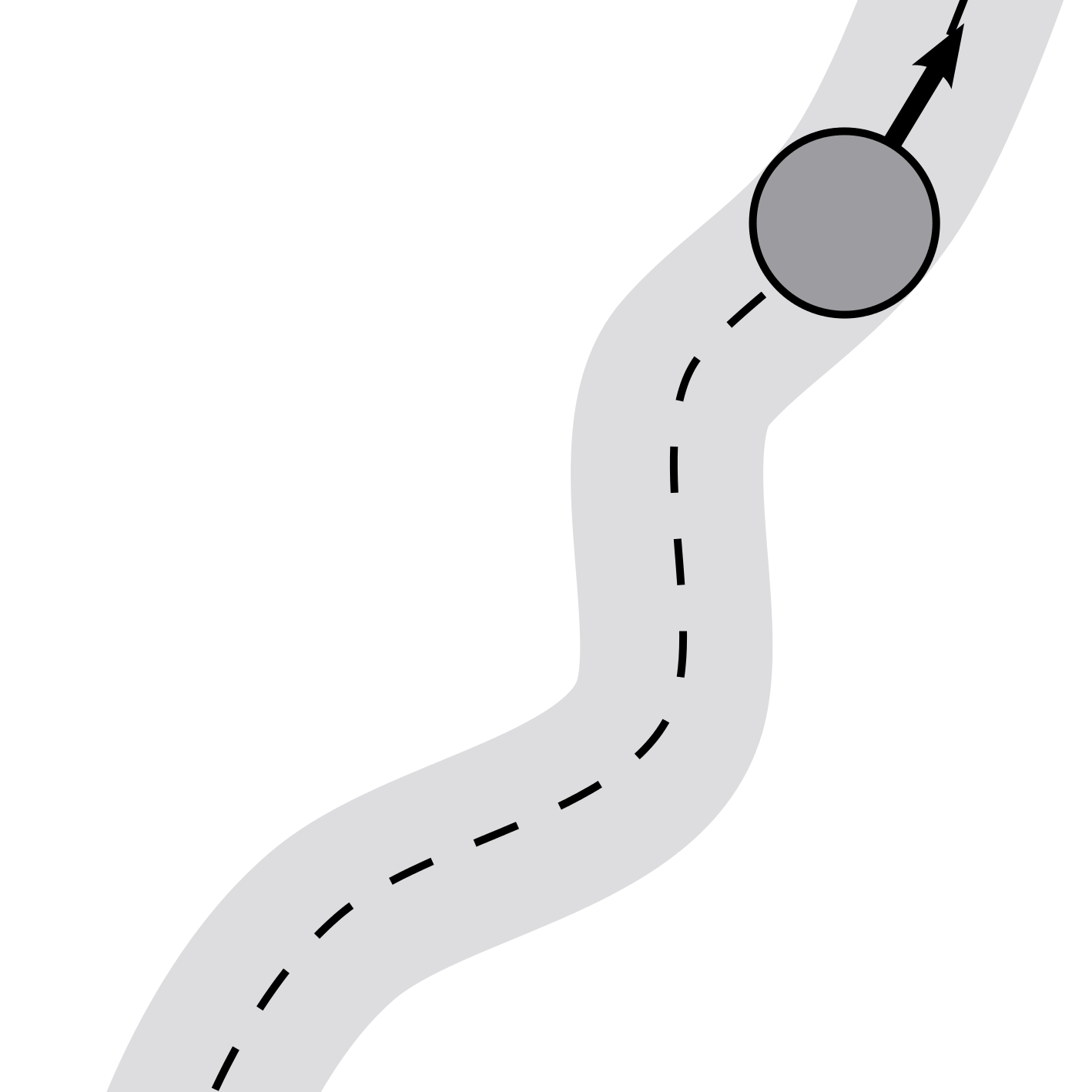
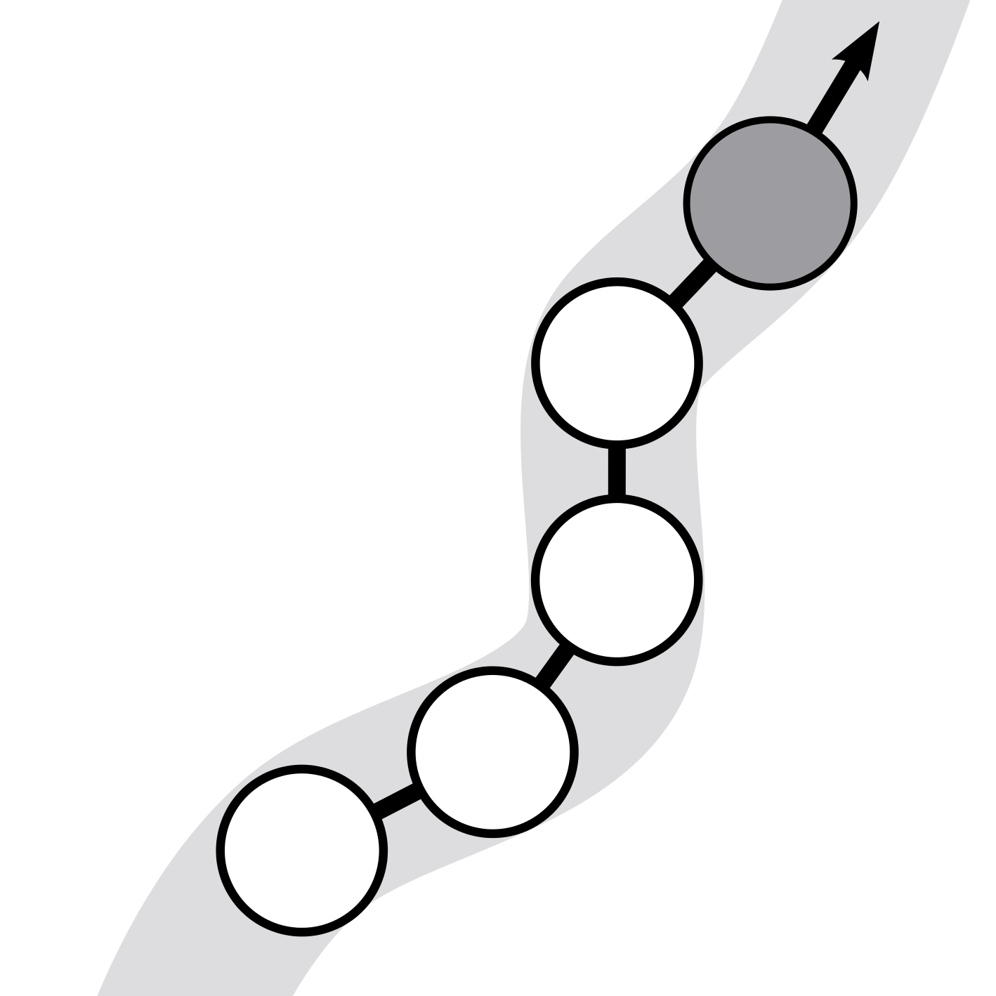
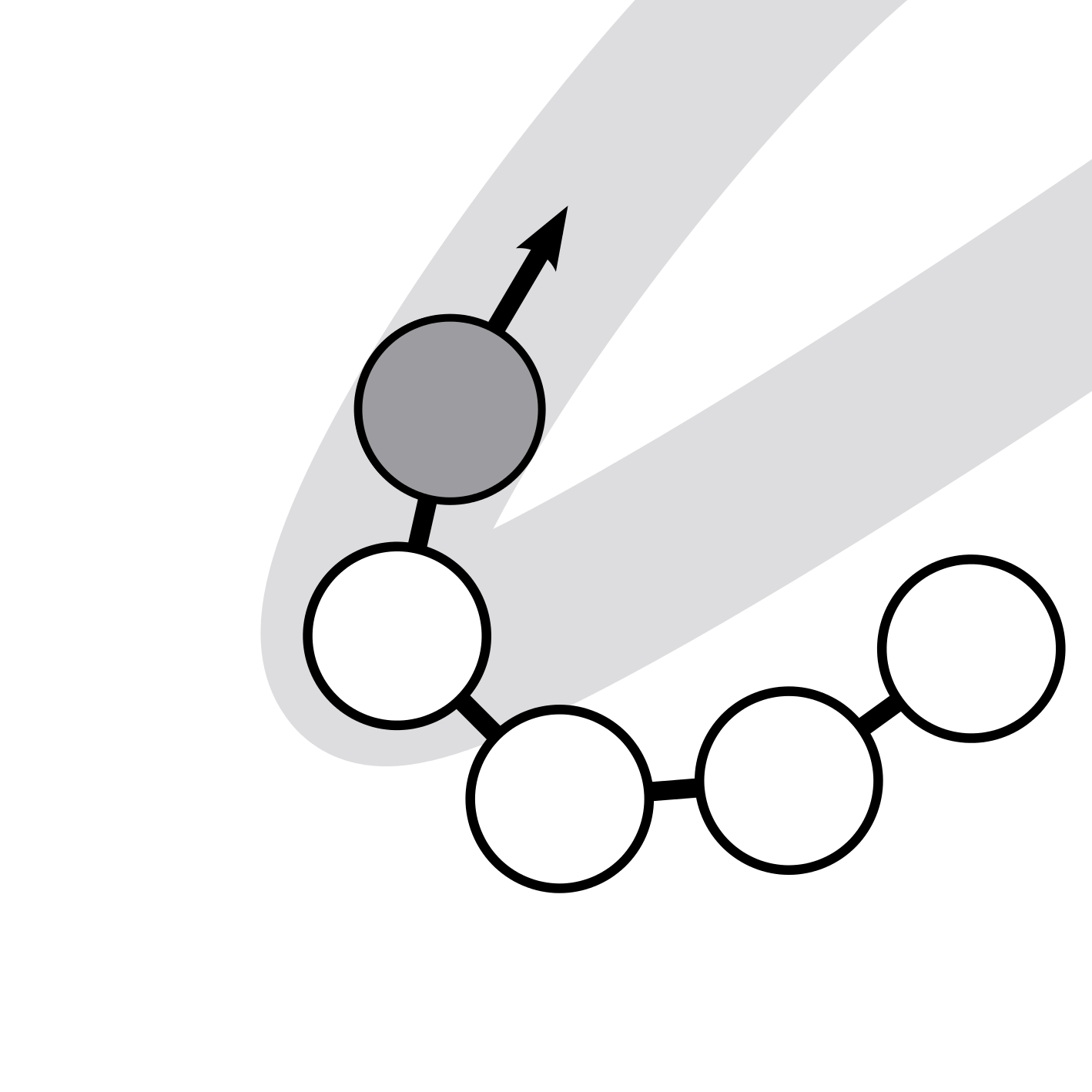
Figure 1: Left: A serial kinematic chain with a root link (grey) and four sublinks (white). Middle left: Root link moves on a curvature constraint path and sweeps a volume (lightgrey). Middle Right: Our algorithm projects the sublinks into the swept volume of the root link. Right: If the curvature of the root link path is too high, the algorithm will fail to project the sublinks.

3 Related Work

Dimensionality reduction of configuration spaces has been extensively studied in the motion planning literature. [3] have used a principal component analysis (PCA) to locally reduce dimensions of small volume and thereby bias random sampling. In the context of manipulation planning, [8] and [4] have introduced the eigengrasp to identify a low-dimensional representation of grasping movements. [9] perform a PCA for a high-dimensional cable robot by sampling deformations. The idea being that many configurations occupy similar volumes in workspace. [10] plan the motion of a cable by first planning a motion for the head. [11] approximate the manifold of self-collision free configurations of the robot, thereby projecting the planning problem onto a lower dimensional sub-manifold in the configuration space.

The approach closest to ours is a subspace decomposition scheme by [5]: an initial path is planned by using only one large subpart of the robot. This initial path is then deformed to account for the remaining links. However, there is no justification or guarantee for being complete.

[12] seem to be the first to introduce the term reducibility of motions. They consider sweeping of disks along a planar curve, whereby the volume of a disk swept along a path is reduced if it is a subset of the swept volume of the same disk swept along another path. We generalize this concept to arbitrary configuration spaces.

In Sec. 5 we establish that sublinks of a serial kinematic chain can be projected into the swept volume if the root link moves on a curvature constrained path. Curvature constrained paths are one of the central objects of study in differential geometry [13]. Our work builds upon work by [14] who compute the reachable regions for curvature-constraint motions inside convex polygons. A generalization of these ideas to 3D has been investigated by [15] who discuss curvature and torsion constraints on space curves in the context of data point approximation.

Our applications consider motion planning for a mechanical snake, a mechanical octopus and a humanoid robot.

The mechanism and locomotion system for snake robots have been studied by [16]. Path planning for snake robots has been investigated in relatively few papers, some of whom are classical approaches using numerical potential fields [17], genetic algorithms [18] or Generalized Voronoi Graphs [19]. The idea of dimensionality reduction for snake robots has been studied by [20], who define a frame consistent with the overall shape of the robot in all configurations. [21] plan a path only for a portion of the snake robot.

Octopus robots have been built by [22] and [23], and its locomotion behavior has been intensively investigated by [24]. However, there has been no demonstration of motion planning for an octopus robot. We concentrate here on motion planning using jet propulsion in narrow environments like a system of pipes.

Motion planning for humanoid robots is a well studied field [25]. Applications range from manipulation planning in kitchen environments [26], contact planning in constrained environments [27][28][29] to ladder climbing tasks [30]. Since general multi-contact planning has a high run-time, researchers have tried to decompose the problem by first planning for simple geometrical shapes. A common approach is first to plan for a sliding box on a floor, then generate footsteps along the box path [3][31]. Such an approach does not work in the environments we consider, and our approach can be seen as a generalization of the decomposition to include the original geometry of the robot.

$\underbrace{\includegraphics[width=104.07024pt,height=208.14049pt]{images/cspace-workspace-irreducible-0-crop.png}}_{\mathcal{C}=\mathbb{R}\times[-\frac{\pi}{2},\frac{\pi}{2}]}\underbrace{\underbrace{\includegraphics[width=52.03247pt]{images/cspace-workspace-irreducible-1-crop.png}}_{V(q_{I}),V(q_{G})}\underbrace{\includegraphics[width=52.03247pt]{images/cspace-workspace-irreducible-2-crop.png}}_{V(\tau_{1})}\underbrace{\includegraphics[width=52.03247pt]{images/cspace-workspace-irreducible-3-crop.png}}_{V(\tau_{2})}\underbrace{\includegraphics[width=52.03247pt]{images/cspace-workspace-irreducible-4-crop.png}}_{V(\tau_{3})}}_{\text{Workspace }\mathcal{W}=\mathbb{R}^{2}}$

Figure 2: Explanatory example of irreducible paths for a $2$-link, $2$-dof robot, which can move along the $y$-axis, and which has one rotational joint between its two links, such that its configuration space is $\mathcal{C}=\mathbb{R}\times[-\frac{\pi}{2},\frac{\pi}{2}]$. Left. Three configuration space paths $\tau_{1},\tau_{2},\tau_{3}$ with $\tau_{1}(0)=\tau_{2}(0)=\tau_{3}(0)=q_{I}$, $\tau_{1}(1)=\tau_{2}(1)=\tau_{3}(1)=q_{G}$. Right. The workspace volume of the starting configurations $q_{I}$, $q_{G}$, and the swept volume of the three paths, whereby we have that $V(\tau_{1})\subset V(\tau_{2})$ and $V(\tau_{1})\subset V(\tau_{3})$, i.e. $\tau_{2}$ and $\tau_{3}$ are reducible by $\tau_{1}$, and $\tau_{1}$ is in fact irreducible. Adapted from [6].

4 Irreducible Paths

The irreducible path is a path of minimal swept volume [6]. In this section we define the irreducible path space, we discuss why the irreducible path space is important (Sec. 4.1), and we investigate the internal structure in Sec. 4.2. Then we prove completeness (Sec. 4.3: If a motion planning algorithm is complete using all paths, then it is complete using only irreducible paths. Finally, we discuss generalizations to dynamically feasible paths in Sec. 4.4.

Let $\mathcal{R}$ be a robot and $\mathcal{C}$ its configuration space, the space of all transformations applicable to $\mathcal{R}$ [1]. Let further $q_{I}\in\mathcal{C}$ be the initial configuration and $q_{G}\in\mathcal{C}$ be the goal configuration.

A motion planning algorithm needs to compute a continuous path between $q_{I}$ and $q_{G}$. The solution space is therefore defined in terms of functional spaces [32, 33]. We first define the space of all paths in $\mathcal{C}$ as

$$\Phi=\{\phi:[0,1]\rightarrow\mathcal{C}|\ \phi\ \text{continuous}\}$$ (1)

We denote the path space between $q_{I}$ and $q_{G}$ as

$$\mathcal{F}_{q_{I},q_{G}}=\{\tau\in\Phi\ |\ \tau(0)=q_{I},\tau(1)=q_{G}\}$$ (2)

For the purpose of this paper we will abbreviate $\mathcal{F}=\mathcal{F}_{q_{I},q_{G}}$ assuming that some $q_{I},q_{G}\in\mathcal{C}$ have been choosen. $\mathcal{F}$ will be called the (full) path space.

If the robot $\mathcal{R}$ follows a path $\tau\in\mathcal{F}$, the body of the robot will sweep a volume. We will denote this swept volume by $V(\tau)$. We then define an irreducible path as

Definition 1 (Irreducible Path).

A path $\tau^{\prime}\in\mathcal{F}$ is called reducible by $\tau$, if there exist $\tau\in\mathcal{F}$ such that $V(\tau)\subset V(\tau^{\prime})$. Otherwise $\tau^{\prime}$ is called irreducible.

All irreducible paths define the irreducible path space.

Definition 2 (Irreducible Path Space).

The space of all irreducible configuration space paths is

$$\mathcal{\hat{I}}=\{\tau\in\mathcal{F}\ |\ \tau\text{ is irreducible}\}$$ (3)

Example 1.

[2-dof robot]

In Fig. 2 we consider a 2-link 2-dof robot, which can move along a straight line and which can rotate its second link around a pivot point. In the second column, the robot is shown in the workspace, once for its initial configuration $q_{I}$, once for its goal configuration $q_{G}$. In the first column, we show three configuration space paths $\tau_{1},\tau_{2},\tau_{3}$ connecting $q_{I}$ to $q_{G}$. On the right we show the corresponding swept volumes in workspace for each path. Applying the definition of irreducibility, we have that $\tau_{2}$ and $\tau_{3}$ are reducible by $\tau_{1}$, while $\tau_{1}$ is irreducible.

4.1 Feasibility of Irreducible Path Space

The importance of the irreducible path space comes from the following claim: If every irreducible path is infeasible, then all paths are infeasible. We prove this claim in Theorem 2.

Let us denote by $\mathbf{E}$ the environment, the set of obstacle regions in $\mathbb{R}^{3}$ [1]. We say that a path $\tau\in\mathcal{F}$ is called feasible in a given environment $\mathbf{E}$, if $V(\tau)\cap\mathbf{E}=\emptyset$.

Theorem 1.

Let $\tau\in\mathcal{\hat{I}},\tau^{\prime}\in\mathcal{F}$ be such that $V(\tau)\subset V(\tau^{\prime})$, i.e. $\tau^{\prime}$ is reducible by $\tau$.

(1) If $\tau$ is infeasible $\Rightarrow$ $\tau^{\prime}$ is infeasible

(2) If $\tau^{\prime}$ is feasible $\Rightarrow$ $\tau$ is feasible

Proof.

Let $S=V(\tau)$ and $S^{\prime}=V(\tau^{\prime})$. (1) Let $S\cap\mathbf{E}\neq\emptyset$, then there exists $v\in S\cap\mathbf{E}$. Since $S\subset S^{\prime}$, $v$ has to be in $S^{\prime}$. But $v$ is also in $\mathbf{E}$, such that $S^{\prime}\cap\mathbf{E}$ has to contain at least $v$ and is therefore not empty.
(2) Let $S^{\prime}\cap\mathbf{E}=\emptyset$. Since $S\subset S^{\prime}$, it follows that $S\cap\mathbf{E}=\emptyset$, which shows that $\tau$ is feasible. ∎

We will say that a path space $\mathcal{F}$ is feasible, if there exists at least one feasible $\tau\in\mathcal{F}$. If there is no feasible $\tau\in\mathcal{F}$, then we say that the space itself is infeasible. By Theorem 1 it follows that

Theorem 2.

If $\mathcal{\hat{I}}$ is infeasible, then $\mathcal{F}$ is infeasible.

Proof.

Let $\tau\in\mathcal{F}$. There are two cases: either (1) there exists a $\tau^{\prime}\in\mathcal{\hat{I}}$ such that $V(\tau^{\prime})\subset V(\tau)$. Then $\tau$ is infeasible by Theorem 1. Or (2) there is no $\tau^{\prime}\in\mathcal{\hat{I}}$ such that $V(\tau^{\prime})\subset V(\tau)$. Then $\tau$ is by definition in $\mathcal{\hat{I}}$ and therefore infeasible.

∎

4.2 Structure of Irreducible Path Space

The irreducible path space $\mathcal{\hat{I}}$ can be partitioned into equivalence classes of paths with equivalent swept volumes.

Definition 3 (Swept Volume Equivalence).

Two irreducible paths $\tau,\tau^{\prime}\in\mathcal{\hat{I}}$ are swept-volume equivalent $\tau\simeq\tau^{\prime}$ if $V(\tau)=V(\tau^{\prime})$

This equivalence relation gives rise to equivalence classes of swept-volume equivalent trajectories. This includes all injective and continuous time-reparameterizations $s:[0,T]\rightarrow[0,1]$ of a path.

Those equivalence classes partition the irreducible path space into a union of disjoint path spaces. This is made precise by taking the quotient space [34] of $\mathcal{\hat{I}}$ as

$$\mathcal{I}=\mathcal{\hat{I}}/{\simeq}$$ (4)

i.e. all swept-volume equivalent paths in $\mathcal{\hat{I}}$ are assigned to exactly one path in the quotient space $\mathcal{I}$.

4.3 Completeness of Irreducible Path Space

We say that a motion planning algorithm is complete in $\mathcal{F}$ if it finds a feasible path in $\mathcal{F}$ if one exists or correctly reports that none exists. Imagine replacing $\mathcal{F}$ by $\mathcal{I}$. We claim that if a motion planning algorithm is complete in $\mathcal{F}$ then it is complete in $\mathcal{I}$ and vice versa.

Theorem 3.

A motion planning algorithm is complete in $\mathcal{I}$ iff it is complete in $\mathcal{F}$

Proof.

To prove equivalence, we need to prove four statements.

1. $\mathcal{I}$ infeasible $\Rightarrow$ $\mathcal{F}$ infeasible,

2. $\mathcal{I}$ feasible $\Rightarrow$ $\mathcal{F}$ feasible,

3. $\mathcal{F}$ infeasible $\Rightarrow$ $\mathcal{I}$ infeasible and

4. $\mathcal{F}$ feasible $\Rightarrow$ $\mathcal{I}$ feasible.

(1) is true by Theorem 2. Statements (2) and (3) are true by inclusion and (4) is true by contraposition of Theorem 2.

∎

In light of Theorem 3 we call the reduction from $\mathcal{F}$ to $\mathcal{I}$ a completeness-preserving reduction.

Example 2.

[Completeness-preserving reduction]

Let us demonstrate the completeness property by the example from Fig. 2. Imagine that $\mathcal{F}$ contains only $\tau_{1},\tau_{2},\tau_{3}$ and $\mathcal{I}$ contains $\tau_{1}$. Imagine further that $\tau_{1}$ is infeasible because it is in collision with some imagined obstacle. Then $\mathcal{I}$ is infeasible. But since $\tau_{2}$ and $\tau_{3}$ are supersets of $\tau_{1}$, they are infeasible too, so we see that $\mathcal{F}$ must be infeasible. Imagine that $\tau_{1}$ is feasible. Then $\mathcal{I}$ is feasible. Since $\mathcal{I}$ is contained in $\mathcal{F}$, $\mathcal{F}$ must be feasible, too.

4.4 Generalization of Irreducible Path to Dynamics

If we consider the dynamics of the robot, we could obtain a situation where the only dynamically feasible path is not irreducible. This could happen if the momentum of the sublinks is crucial to solve a task. While in this paper we focus on collision-free paths where the dynamics are not considered, the concept of an irreducible path can in principle be generalized to incorporate dynamically feasible paths.

A path is dynamically feasible if it is a solution to the equation of motion of the robot. We define $\mathcal{F}_{D}$ as the subspace of all paths being dynamically feasible. Combined with the concept of an irreducible path we obtain

Definition 4 (Dynamically Irreducible Path).

A path $\tau^{\prime}\in\mathcal{F}_{D}$ is called dynamically reducible by $\tau$, if there exist $\tau\in\mathcal{F}_{D}$ such that $V(\tau)\subset V(\tau^{\prime})$. Otherwise $\tau^{\prime}$ is called dynamically irreducible.

We note that the previous discussion of completeness analogously applies to dynamically irreducible paths. In this paper, however, we consider only the non-dynamical case. The characterization of the dynamically irreducible path space is left for future work.

5 Irreducible Motion Planning for Serial Kinematic Chains

As an application, let us approximate the irreducible path space of a serial kinematic chain. A serial kinematic chain is an alternating sequence of $N+1$ links and $N$ joints as examplified in Fig. 3.

We will call the first link in the chain the root link and we will call the remaining $N$ links sublinks. Our assumptions are that all joints are either revolute or spherical, that the volume of the root link is bigger or equal to the volume of the sublinks, and that the root link is free-floating.

Under those assumptions, our main idea is the following: if the root link follows a curvature-constrained path, then the sublinks can be projected into the swept volume of the root link along the path. Each curvature-constrained path is thereby associated with an irreducible path.

Motion planning for a serial kinematic chain is thereby decomposed into two parts: first, conduct curvature-constrained motion planning for the root link, and second, project the sublinks into the swept volume of the root link. We will first describe how to conduct motion planning for the root link, and then describe how to construct an algorithm to project the sublinks.

5.1 Motion Planning for the Root Link

The root link is a free-floating rigid body. Our goal is to plan a path for the root link under a certain maximum curvature constraint $\kappa$. Since the swept volume of a path is invariant to reparameterization of the path (Sec. 4.2), we can compute the path where the robot moves at unit speed.

Planning with a curvature-constrained functional space using constant unit speed is equivalent to planning a path for a non-holonomic rigid body subject to differential constraints describing forward non-slipping motions. This is equivalent to the model of Dubin’s car, which can be solved in both 2d and 3d using kinodynamic planning [1].

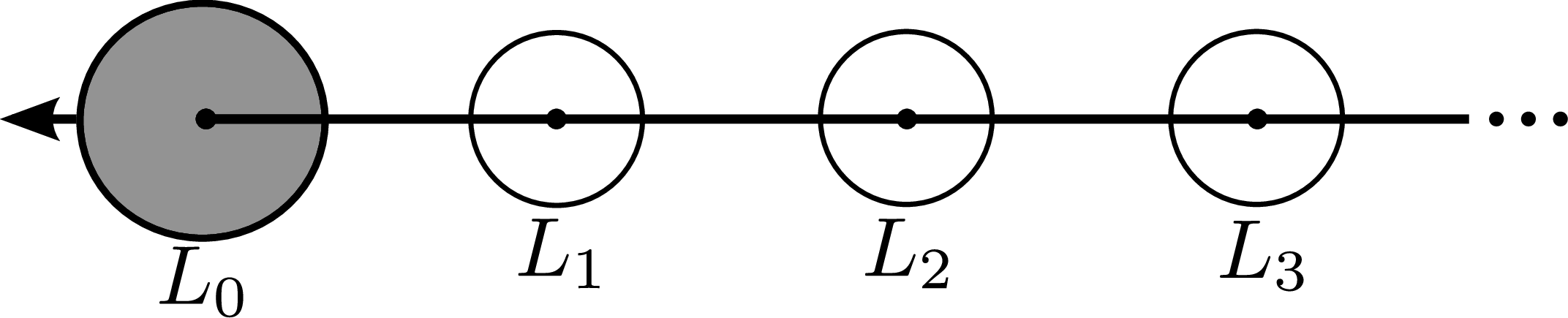
Figure 3: A serial kinematic chain with $L_{0}$ being the root link, and $L_{1},L_{2},\cdots$ are called the sublinks.

In 2d, the configuration space of the root link is $SE(2)$ with $q=\left(x,y,\theta\right)^{T}$ and the differential model at unit speed is given by

$$\dot{x}=\cos\theta$$ (5)

$$\dot{y}=\sin\theta$$

$$\dot{\theta}=u$$

where the control space is defined by the steering angle $u\in[-\operatorname{atan}(\kappa),\operatorname{atan}(\kappa)]$ with $\kappa$ being the curvature constraint. In 3d, the configuration space of the root link is $SE(3)$ and the differential model is similar to a driftless airplane given by

$$\dot{q}=q\left(X_{1}+\sum_{i=4}^{6}u_{i}X_{i}\right)$$ (6)

where

$$X_{1}=\left[\begin{smallmatrix}0&0&0&1\\ 0&0&0&0\\ 0&0&0&0\\ 0&0&0&0\end{smallmatrix}\right] X_{2}=\left[\begin{smallmatrix}0&0&0&0\\ 0&0&0&1\\ 0&0&0&0\\ 0&0&0&0\end{smallmatrix}\right] X_{3}=\left[\begin{smallmatrix}0&0&0&0\\ 0&0&0&0\\ 0&0&0&1\\ 0&0&0&0\end{smallmatrix}\right]$$

$$X_{4}=\left[\begin{smallmatrix}0&-1&0&0\\ 1&0&0&0\\ 0&0&0&0\\ 0&0&0&0\end{smallmatrix}\right] X_{5}=\left[\begin{smallmatrix}0&0&1&0\\ 0&0&0&0\\ -1&0&0&0\\ 0&0&0&0\end{smallmatrix}\right] X_{6}=\left[\begin{smallmatrix}0&0&0&0\\ 0&0&-1&0\\ 0&1&0&0\\ 0&0&0&0\end{smallmatrix}\right]$$

is a basis for $\mathfrak{se}(3)$, the Lie algebra of $SE(3)$[35]. The controls $u_{4},u_{5}\in[-\operatorname{atan}(\kappa),\operatorname{atan}(\kappa)]$ and $u_{6}\in\mathbb{R}$ are the yaw, pitch, and roll steering angles and $X_{1}$ represents the forward motion at unit speed.

In Appendix A we analytically compute the curvature $\kappa$ for a serial chain in the plane using disk-shaped links. In all our experiments we have computed $\kappa$ as if the chain would be 2-dimensional. We have observed that this worked well in experiments. However, further research needs to investigate the correctness of this claim.

5.2 Algorithm to Project Sublinks into Swept Volume of Root Link

Let $\tau:[0,1]\rightarrow SE(3)$ be a path for the root link of the serial chain, and let $\tau$ be constrained by having a maximal curvature $\kappa$ such that $\kappa(s)\leq\kappa$ for all $s\in[0,1]$. Given $\tau$, let $V(\tau)$ be the swept volume of the root link. We claim that for a given $\kappa$, we can find at least one configuration of the sublinks such that the swept volume of the sublinks is a subset of $V(\tau)$. In Section 5.2.2 we discuss the correctness of this claim, and in Appendix A we provide a proof for an N-dimensional serial kinematic chain in the plane.

In this section, we develop the curvature projection algorithm, which takes as input a path of the root link and provides one configuration of the sublinks. Our algorithm approximates the serial chain by a set of spheres of radius $\delta_{0},\cdots,\delta_{N}$ which are connected by lines of length $l_{0},\cdots,l_{N-1}$. The serial chain has $N$ joints centered at each of the spheres. Each joint is described by two parameters $(\theta_{i},\gamma_{i})$, whereby $\theta_{i}$ represents the rotation around the normal unit vector centered at the previous link and $\gamma_{i}$ represents the rotation around the binormal unit vector centered at the previous link. The system is then represented by the position and orientation of the root link in space, i.e. $SE(3)$, plus its joint configurations $\boldsymbol{\theta}=\{\theta_{1},\cdots,\theta_{N}\}$ and $\boldsymbol{\gamma}=\{\gamma_{1},\cdots,\gamma_{N}\}$.

5.2.1 Algorithmic Description

Data: $\tau,\tau^{\prime},\tau^{\prime\prime},\delta_{0:N}$, $l_{1:N},\Delta t$

Result: $\theta_{1:N},\gamma_{1:N}$

1 $\mathbf{e}_{1}\leftarrow\tau^{\prime}(0)$;

2 $\mathbf{e}_{2}\leftarrow\tau^{\prime\prime}(0)$;

3 $\mathbf{e}_{3}\leftarrow\tau^{\prime}(0)\times\tau^{\prime\prime}(0)$;

4

5$s_{last}\leftarrow 0$;

6

7$\mathbf{R}\leftarrow\begin{pmatrix}\mathbf{e}_{1}\cdot\mathbf{e}_{x}&\mathbf{e}_{2}\cdot\mathbf{e}_{x}&\mathbf{e}_{3}\cdot\mathbf{e}_{x}\\ \mathbf{e}_{1}\cdot\mathbf{e}_{y}&\mathbf{e}_{2}\cdot\mathbf{e}_{y}&\mathbf{e}_{3}\cdot\mathbf{e}_{y}\\ \mathbf{e}_{1}\cdot\mathbf{e}_{z}&\mathbf{e}_{2}\cdot\mathbf{e}_{z}&\mathbf{e}_{3}\cdot\mathbf{e}_{z}\end{pmatrix}$;

8

9for  $i\leftarrow 1$ to $N$  do

10      

11      $s_{next}\leftarrow s_{last}$;

12       while $\|\tau(s_{next})-\tau(s_{last})\|\leq l_{i}$ do

13             $s_{next}\leftarrow s_{next}-\Delta t$

14      $\tau_{n}\leftarrow\tau(s_{next})$;

15      

16      $p_{I}\leftarrow\tau(s_{next})-\tau(s_{last})$;

17       $p_{W}\leftarrow\mathbf{R}^{T}p_{I}$;

18       $x_{L}\leftarrow(-1,0,0)^{T}$;

19      

20      $p_{xy}\leftarrow p_{W}-(p_{W}^{T}\mathbf{e}_{z})\mathbf{e}_{z}$;

21       $p_{zx}\leftarrow p_{W}-(p_{W}^{T}\mathbf{e}_{y})\mathbf{e}_{y}$;

22       $\theta_{i}\leftarrow\operatorname{acos}(\frac{p_{xy}^{T}x_{L}}{\|p_{xy}\|\|x_{L}\|})$;

23       $\gamma_{i}\leftarrow\operatorname{acos}(\frac{p_{zx}^{T}x_{L}}{\|p_{zx}\|\|x_{L}\|})$;

24      

25      if $p_{W}^{T}\mathbf{e}_{z}<0$ then

26             $\gamma_{i}\leftarrow-\gamma_{i}$;

27            

28      if $p_{W}^{T}\mathbf{e}_{y}>0$ then

29             $\theta_{i}\leftarrow-\theta_{i}$;

30            

31      

32      $\mathbf{R}\leftarrow\mathbf{R}\cdot\mathbf{R}_{Y}(\gamma_{i})\cdot\mathbf{R}_{Z}(\theta_{i})$;

33      

34      $\mathbf{e}_{1}\leftarrow\mathbf{R}\mathbf{e}_{x}$;

35       $\mathbf{e}_{2}\leftarrow\mathbf{R}\mathbf{e}_{y}$;

36       $\mathbf{e}_{3}\leftarrow\mathbf{R}\mathbf{e}_{z}$;

37       $s_{last}\leftarrow s_{next}$;

38      

Algorithm 1 Irreducible Curvature Projection Algorithm

The resulting algorithm is described in Fig. 1. It takes as input the path of the root link $\tau$, its first and second derivative $\tau^{\prime}$ and $\tau^{\prime\prime}$, the size of the spheres $\delta_{0:N}$ for the root link and the $N$ sublinks, and the length of the links $l_{1:N}$. It outputs the configurations of the sublinks $\theta_{1:N},\gamma_{1:N}$, such that each sublink is inside the swept volume of the root link. We assume that there exists a world frame $O$ with basis $\mathbf{e}_{x},\mathbf{e}_{y},\mathbf{e}_{z}$. Starting from $s_{last}=0$ we compute a frame $S_{0}$ centered at the root link with orthonormal basis $\mathbf{e}_{1},\mathbf{e}_{2},\mathbf{e}_{3}$ (Line 1-4), and we compute the rotational transformation matrix $\mathbf{R}$ between $O$ and $S_{0}$ (Line 5). Then for each sublink (Line 6), we start at $s_{last}$, and we follow $\tau$ backwards until the distance between $\tau(s_{next})$ and $\tau(s_{last})$ is equal to $l_{i}$ (Line 7-9). This position marks the position of the $i$-th sublink. We mark the position as $s_{next}$ (Line 10), we compute the vector from $S$ to $s_{next}$ (Line 11), and we rotate this vector into the world frame $O$ (Line 12). Then we compute the angle of the vector to the $xy$ and the $zx$ plane, respectively (Line 13-21). Those angles give the configuration $\theta_{i},\gamma_{i}$ of sublink $i$. Finally, we rotate the rotation matrix $\mathbf{R}$ correspondingly (Line 22) to obtain a new frame $S_{i}$ centered at link $i$ (Line 23-26). The algorithm is iterated until all $N$ sublinks have been placed in that manner. See also Fig. 4 for a visualization of the algorithm in a 2D setting.

Figure 4: Given a path $\tau\in\mathcal{F}_{\kappa_{N}}$, we can analytically compute the joint configurations, such that sublinks of the serial kinematic chain are reduced, i.e. they are inside of the swept volume of $\tau\oplus L_{0}$.

5.2.2 Complexity and Correctness

The complexity of the algorithm is $\mathcal{O}(N)$, $N$ being the number of sublinks. In Appendix A we prove the correctness of the algorithm for a serial kinematic chain in 2D, whereby we assume that the lengths between joints is equidistant. The proof first verifies the correctness of the algorithm of a chain with $N=1$ sublinks and then generalizes this result to arbitrary sublinks $N>1$. The proof of correctness of the algorithm with arbitrary lengths and with spherical joints in 3D is subject of further research.

6 Experiments

We will show that the concept of an irreducible path space can be applied to any motion planning algorithm taking curvature constraints into account, and that each planning algorithm using the irreducible path space outperforms the same motion planning algorithm using the space of all continuous paths.

We performed seven experiments to test our hypothesis. Our first three experiments are planning scenarios for an idealized serial kinematic chain in a 2d maze, a 2d rock environment and a 3d rock environment. We compared the kinodynamic Rapidly-exploring Random-Tree (RRT) [36] algorithm both using the original space and the irreducible path space. In the fourth experiment we plan a path for a mechanical snake in a turbine environment. We compared four different motion planning algorithms: RRT, Path-Directed Subdivision Tree planner (PDST) [37], Kinodynamic motion Planning by Interior-Exterior Cell Exploration (KPIECE) [38] and Stable Sparse Tree (SST) [39]. In the fifth experiment we plan a path for a mechanical octopus in a pipe environment, using the same four algorithms. In all those experiments we assume that the head of the robot can be independently controlled. In the sixth and seventh experiments we plan a path for a humanoid robot, first in a room with doors of different heights and second on a floor with a hole in a wall.

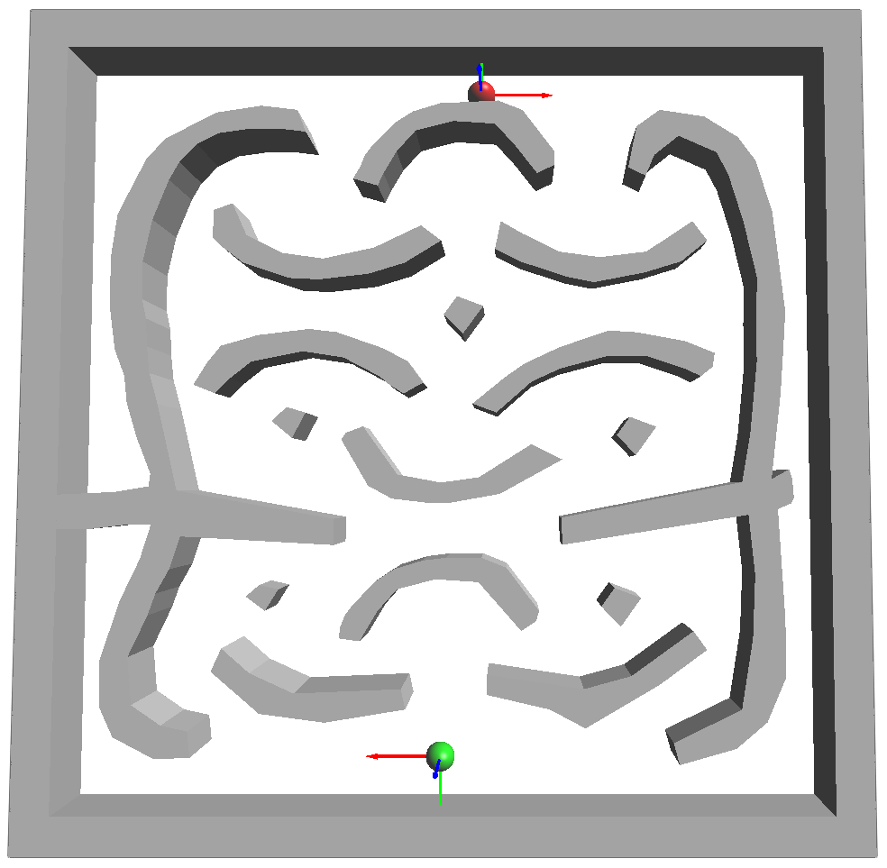
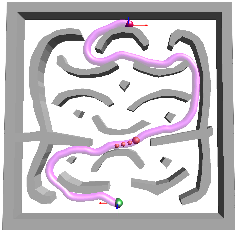
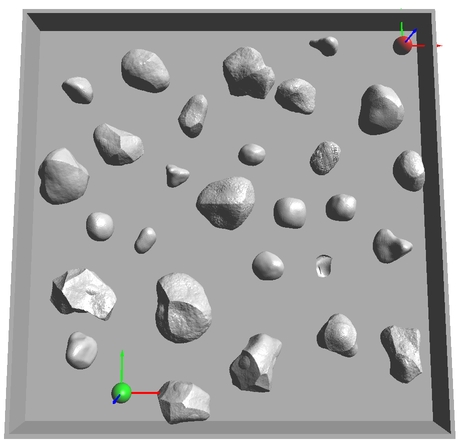
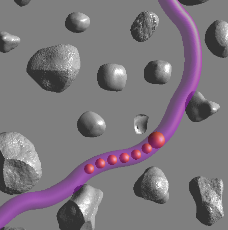
Figure 5: Serial kinematic chain in 2D (From Left to Right). Image 1 and 2 show the start and goal configuration of Experiment $1$ and the swept volume along one irreducible solution path, respectively. Image 3 and 4 show a serial kinematic chain in an environment filled with rocks. We show the start and goal configuration and the swept volume along a solution path, respectively.

For each experiment we specify the values of the serial kinematic chain, the maximum curvature $\kappa$, the joint limit $\theta^{L}$, the size of the root link $\delta_{0}$ and the number of sublinks $N$. Each experiment is repeated $M$ times and it is terminated if a time threshold $T$ is reached or if a goal region of size $\epsilon_{\text{goal}}$ around the goal configuration is reached.

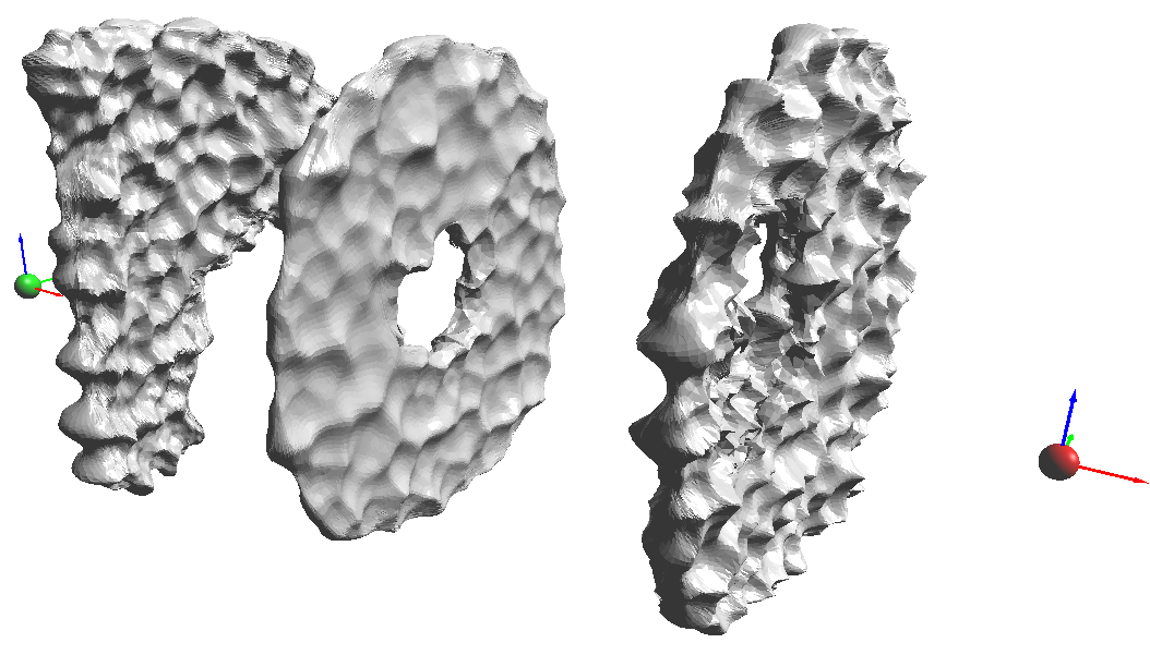
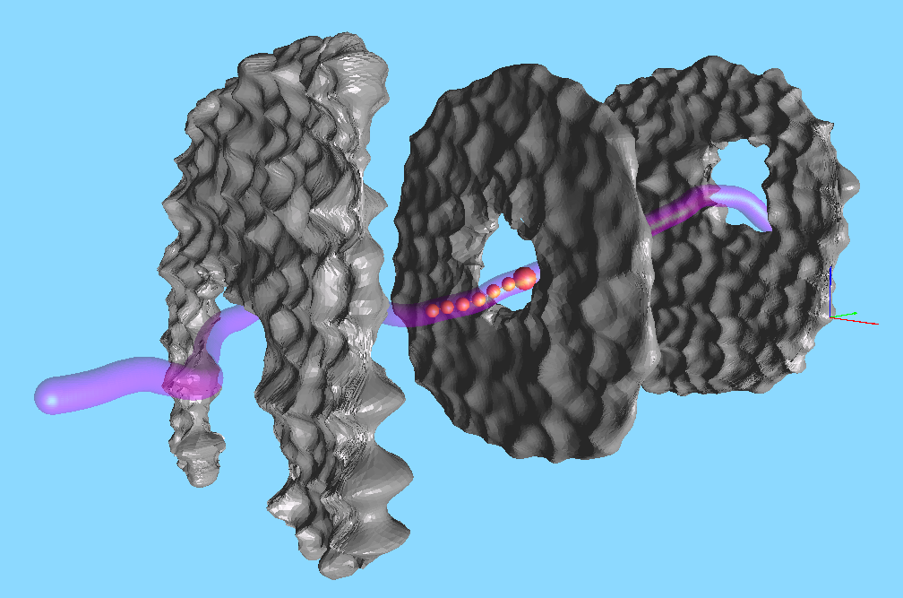
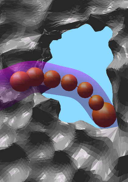
Figure 6: Planning for the root link of a serial kinematic chain on $SE(3)$. Left: 3d rocks environment with starting position (green) and goal position (red). Middle: An irreducible path found by RRT [Irreducible]. The swept volume of the root link is shown in magenta. The position of the sublinks is an output of the curvature projection algorithm. Right: Close-up of a position of the robot along the irreducible path, showing how the sublinks are inside the swept volume of the root link.

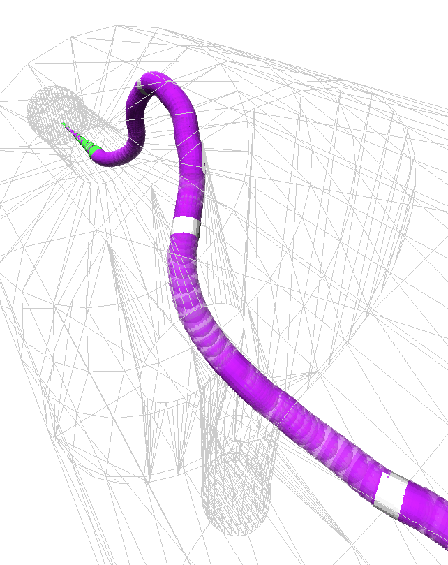
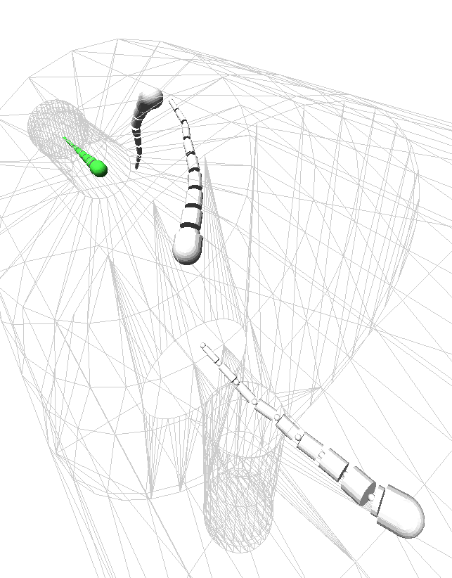
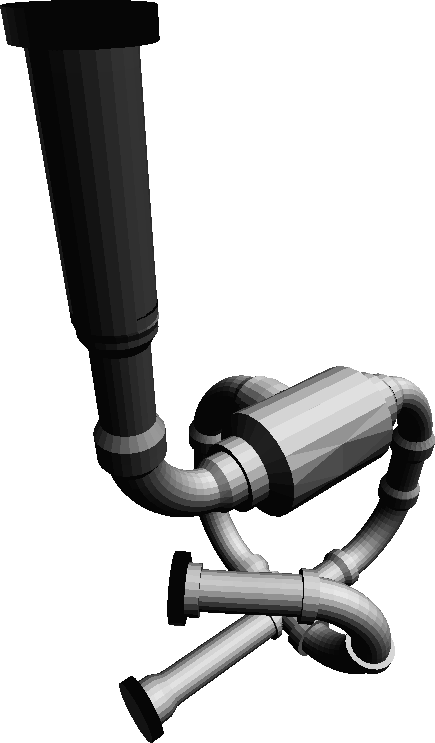
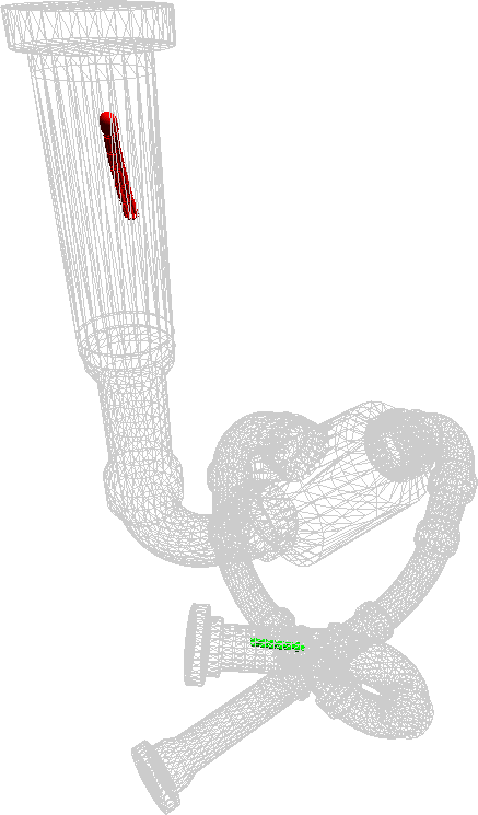
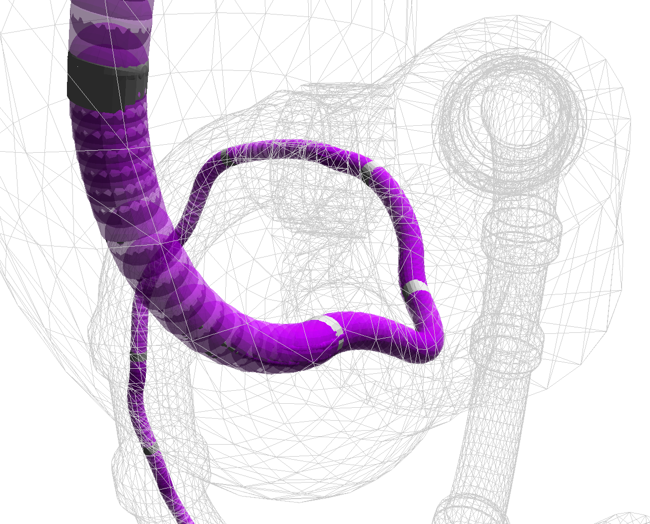
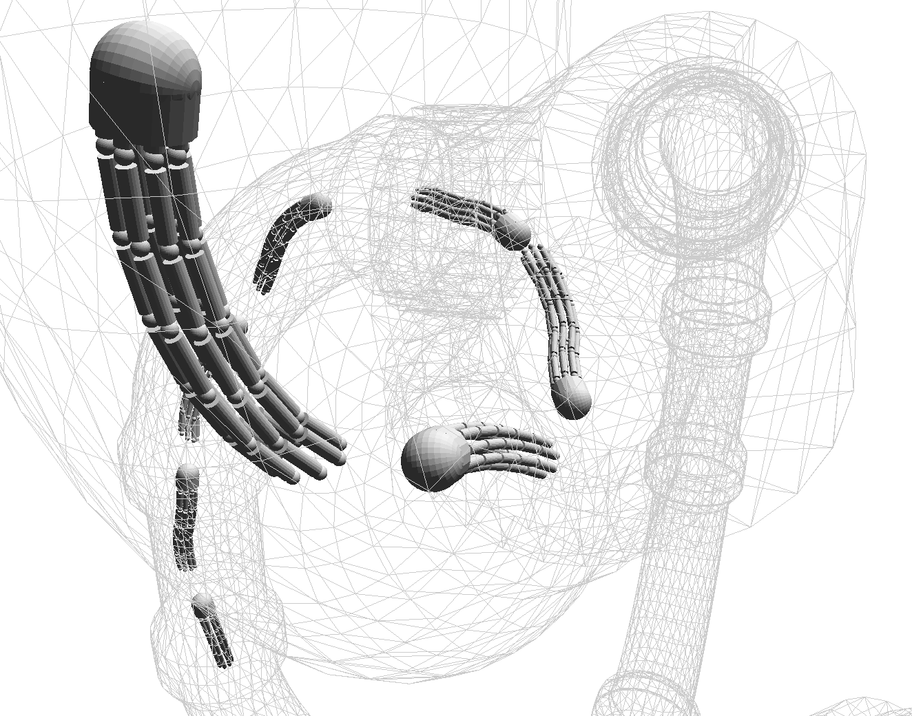
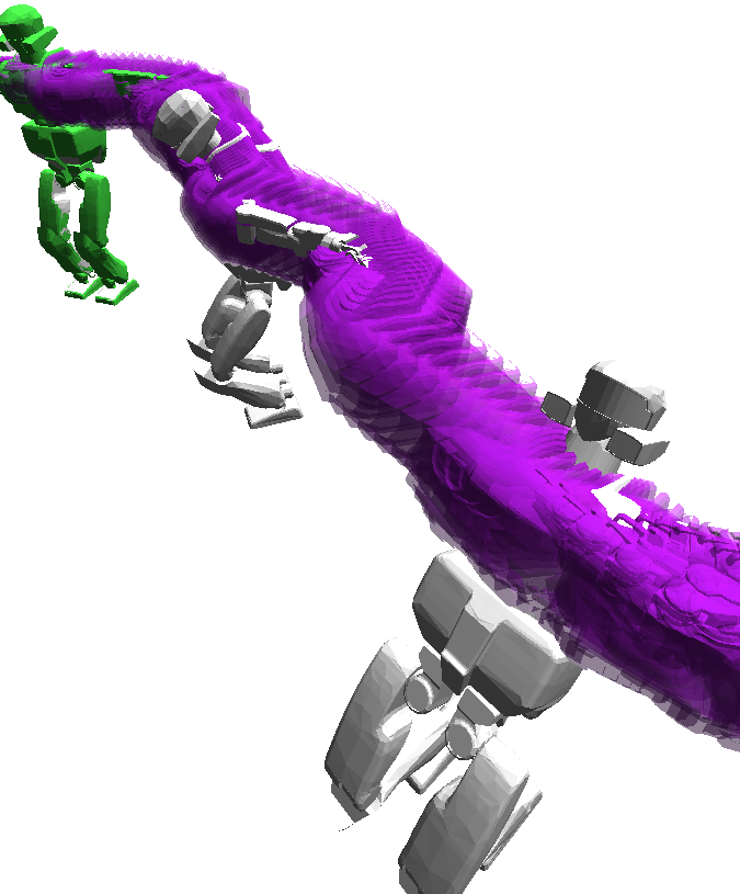
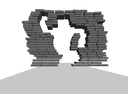
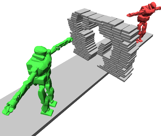
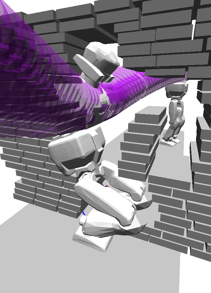
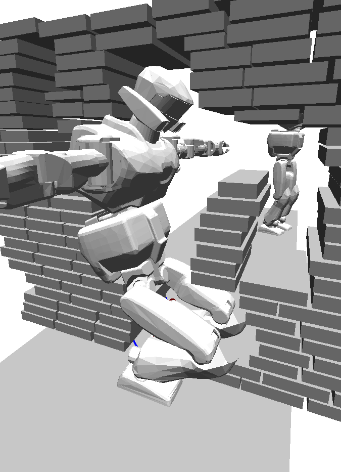
Figure 7: Visualization of the motion planning experiments. For each experiment we show the environment (column 1), the start configuration in green and the goal configuration in red (column 2), the close up of a swept volume of one irreducible solution path in magenta (column 3) and milestones along the swept volume in gray (column 4). The first row (Experiment 4) shows a mechanical snake in a turbine environment. The second row (Experiment 5) is a mechanical octopus in a pipe environment. The third row (Experiment 6) shows a humanoid robot moving sideways through a room with doors of different height. For better visualization, only the swept volume of the chest is visualized. The fourth row (Experiment 7) shows the same humanoid robot moving sideways through a hole in a wall shaped according to the geometry of the robot.

6.1 Experiment 1: Serial Kinematic Chain in 2D maze

Our first experiment is a 2d maze environment as depicted in Fig. 5, where a serial kinematic chain has to be moved from a given start to a given goal configuration. We assume that the root link can be independently actuated. The configuration space is $SE(2)\times\mathbb{R}^{3}$. We compare RRT using the full space of paths with RRT [Irreducible] using the space of irreducible paths. We report on the success rate, the average time to plan, and the standard deviation of the planning algorithm in Tab. 1. It can be seen that RRT [Irreducible] has a lower planning time of one order of magnitude. The parameters used were $\kappa=1$, $\theta^{L}=\frac{\pi}{2}$, $\delta_{0}=0.23$, $N=3$, $M=100$, $T=3600$s and $\epsilon_{\text{goal}}=0.1$.

6.2 Experiment 2: Serial Kinematic Chain in 2D rock environment

Our second experiment is a 2d rock environment as depicted in Fig. 5. We compared again RRT with RRT [Irreducible]. The results are reported in Table 1 and show that RRT [Irreducible] using the irreducible path space outperforms RRT using the space of continuous paths. The parameters used were $\kappa=1$, $\theta^{L}=\frac{\pi}{2}$, $\delta_{0}=0.23$, $N=6$, $M=100$, $T=3600$s and $\epsilon_{\text{goal}}=0.1$.

6.3 Experiment 3: Serial Kinematic Chain in 3D rock environment

Our third experiment changes the 2d rock environment into a 3d rock environment, where the serial kinematic chain has to move through a series of holes to reach a target. The configuration manifold is $SE(3)\times\mathbb{R}^{12}$.

We compare again RRT and RRT [Irreducible], results shown in Table 1. Fig. 6 shows a time instance from one successful run of the RRT [Irreducible], where the swept volume of the planned motion for the head is shown in magenta, and the sublinks are shown as the results of our projection algorithm. Parameters used were $\kappa=1$, $\theta^{L}=\frac{\pi}{2}$, $\delta_{0}=0.23$, $N=6$, $M=100$, $T=3600$s and $\epsilon_{\text{goal}}=0.1$.

6.4 Experiment 4: Mechanical snake in 3D turbine environment

In the fourth experiment we use a mechanical snake which has to move through a 3D turbine environment. Inside the turbine there is a narrow hole through which the snake has to move. The dimensionality of the configuration space is $SE(3)\times\mathbb{R}^{16}$. We compare RRT, PDST, KPIECE and SST with the full path space against the same algorithms using the irreducible path space. The results in Table 1 show that each original algorithm is outperformed by the same algorithm using the irreducible path space. The overall best average computation time has been achieved by KPIECE [Irreducible]. The environment, the start and goal configuration, a swept volume along the one irreducible solution path and a close up of milestones are shown in row $1$ of Fig. 7. The parameters are $\kappa=1.57$, $\theta^{L}=\frac{\pi}{4}$, $\delta_{0}=0.1$, $N=8$, $M=100$, $T=1200$s and $\epsilon_{\text{goal}}=0.5$.

6.5 Experiment 5: Mechanical octopus in 3D pipe environment

In the fifth experiment we use a mechanical octopus which has $8$ arms with each $5$ sublinks leading to a configuration space of dimensionality $SE(3)\times\mathbb{R}^{80}$. For the irreducible path space we compute a path for the head on $SE(3)$, then project all the remaining links into the swept volume of the head by applying the curvature projection algorithm on each arm individually. Results in Table 1 indicate that the original problem was too difficult to be solvable by any algorithm. However, the irreducible path space variations can find a solution with PDST [Irreducible] achieving the best average computation time while succeding in $100$ percent of the cases. Row $2$ of Fig. 7 visualizes the environment and one solution path. The parameters used were $\kappa=2.66$, $\theta^{L}=\frac{\pi}{2}$, $\delta_{0}=0.1$, $N=5$, $M=100$, $T=1200$, and $\epsilon_{\text{goal}}=1.0$.

6.6 Experiment 6: Humanoid Robot in Room environment

In the sixth experiment we consider motion planning for the sideways motion of a humanoid robot as shown in row $3$ of Fig. 7. This can be helpful to estimate if a humanoid robot can potentially fit through a door or a small opening. The environment consists of two doors with different heights. We make the assumption that the robot slides on the planar floor leading to the configuration space $SE(2)\times\mathbb{R}^{19}$. We apply the idea of the irreducible path space to the chest of the robot, such that the arms of the robot behave like the sublinks of the serial kinematic chain. Since each arm has $7$ dofs, the resulting dimensionality is $SE(2)\times\mathbb{R}^{5}$. As shown in Table 1 each algorithm using the irreducible path space outperforms the same algorithm using the full path space. The best algorithm in terms of average computation time is RRT [Irreducible] achieving $100$ percent success rate. A solution path is shown in row $3$ of Fig. 7, showing how the arms have been projected into the swept volume of the chest. The parameters are $\kappa=2.66$, $\theta^{L}=\frac{\pi}{2}$, $\delta_{0}=0.1$, $N=3$, $M=100$, $T=1200$, and $\epsilon_{\text{goal}}=0.5$.

6.7 Experiment 7: Humanoid Robot in Hole in Wall environment

The last experiment is similar to experiment $6$ with a more challenging environment. The humanoid robot has to move through a hole in a wall which is shaped according to the robot’s geometry. This is difficult , since a possible solution path has to overcome the narrow passage in the configuration space. Due to this difficulty we only used the best algorithm from experiment $6$, the RRT using $M=10$ runs with a timelimit of $T=86400$s or $24$h. We compared the performance of RRT [Irreducible] with RRT as shown in Table 1. It can be seen that RRT [Irreducible] is able to find a path although it takes on average $100$ minutes to obtain a solution. RRT was not able to find a solution in the given time limit. A solution path is shown in row $4$ of Fig. 7 after a shortcut procedure was applied. This experiment is a reimplementation of the experiment conducted in [6].

Table 1: Results of the seven experiments. Each algorithm used is compared between its original version and the irreducible version using the irreducible path space.

Algorithm	Manifold	Sampling Manifold	Success ($\%$)	Time($s$)
Serial Kinematic Chain — Maze 2D Environment (M=100, T=3600)
RRT	$SE(2)\times\mathbb{R}^{3}$	$SE(2)\times\mathbb{R}^{3}$	100	174	.70	$\pm\$	177	.07
RRT [Irreducible]		$SE(2)$	100	17	.92	$\pm\$	9	.47
Serial Kinematic Chain — Rock 2D Environment (M=100, T=3600)
RRT	$SE(2)\times\mathbb{R}^{6}$	$SE(2)\times\mathbb{R}^{6}$	100	115	.63	$\pm\$	148	.75
RRT [Irreducible]		$SE(2)$	100	4	.24	$\pm\$	3	.17
Serial Kinematic Chain — Rocks 3D Environment (M=$100$, T=$3600$s)
RRT	$SE(3)\times\mathbb{R}^{16}$	$SE(3)\times\mathbb{R}^{16}$	0	3600	.00	$\pm\$	0	.0
RRT [Irreducible]		$SE(3)$	100	531	.40	$\pm\$	623	.32
Mechanical Snake — Turbine Environment (M=$100$, T=$1200$s)
KPIECE	$SE(3)\times\mathbb{R}^{16}$	$SE(3)\times\mathbb{R}^{16}$	52	625	.74	$\pm\$	566	.55
KPIECE [Irreducible]		$SE(3)$	100	13	.42	$\pm\$	64	.83
PDST	$SE(3)\times\mathbb{R}^{16}$	$SE(3)\times\mathbb{R}^{16}$	15	1120	.35	$\pm\$	208	.10
PDST [Irreducible]		$SE(3)$	96	95	.43	$\pm\$	250	.40
RRT	$SE(3)\times\mathbb{R}^{16}$	$SE(3)\times\mathbb{R}^{16}$	46	813	.32	$\pm\$	481	.19
RRT [Irreducible]		$SE(3)$	90	352	.40	$\pm\$	392	.35
SST	$SE(3)\times\mathbb{R}^{16}$	$SE(3)\times\mathbb{R}^{16}$	51	811	.40	$\pm\$	462	.88
SST [Irreducible]		$SE(3)$	87	360	.60	$\pm\$	436	.69
Mechanical Octopus — Pipes Environment (M=$100$, T=$1200$s)
KPIECE	$SE(3)\times\mathbb{R}^{80}$	$SE(3)\times\mathbb{R}^{80}$	0	1200	.00	$\pm\$	0	.0
KPIECE [Irreducible]		$SE(3)$	100	308	.72	$\pm\$	60	.78
PDST	$SE(3)\times\mathbb{R}^{80}$	$SE(3)\times\mathbb{R}^{80}$	0	1200	.00	$\pm\$	0	.0
PDST [Irreducible]		$SE(3)$	100	23	.88	$\pm\$	14	.26
RRT	$SE(3)\times\mathbb{R}^{80}$	$SE(3)\times\mathbb{R}^{80}$	0	1200	.00	$\pm\$	0	.0
RRT [Irreducible]		$SE(3)$	97	215	.05	$\pm\$	270	.08
SST	$SE(3)\times\mathbb{R}^{80}$	$SE(3)\times\mathbb{R}^{80}$	0	1200	.00	$\pm\$	0	.0
SST [Irreducible]		$SE(3)$	99	110	.10	$\pm\$	207	.82
Humanoid Robot HRP-2 — Doors (M=$100$, T=$1200$s)
KPIECE	$SE(2)\times\mathbb{R}^{19}$	$SE(2)\times\mathbb{R}^{19}$	0	1200	.00	$\pm\$	0	.0
KPIECE [Irreducible]		$SE(2)\times\mathbb{R}^{5}$	31	1019	.67	$\pm\$	316	.00
PDST	$SE(2)\times\mathbb{R}^{19}$	$SE(2)\times\mathbb{R}^{19}$	0	1200	.00	$\pm\$	0	.0
PDST [Irreducible]		$SE(2)\times\mathbb{R}^{5}$	19	1051	.05	$\pm\$	336	.31
RRT	$SE(2)\times\mathbb{R}^{19}$	$SE(2)\times\mathbb{R}^{19}$	40	834	.38	$\pm\$	467	.78
RRT [Irreducible]		$SE(2)\times\mathbb{R}^{5}$	100	166	.36	$\pm\$	181	.99
SST	$SE(2)\times\mathbb{R}^{19}$	$SE(2)\times\mathbb{R}^{19}$	59	746	.34	$\pm\$	426	.11
SST [Irreducible]		$SE(2)\times\mathbb{R}^{5}$	99	175	.92	$\pm\$	199	.39
Humanoid Robot HRP-2 — Wall (M=10, T=$86400$s=$24$h)
RRT	$SE(2)\times\mathbb{R}^{19}$	$SE(2)\times\mathbb{R}^{19}$	0	86400	.00	$\pm\$	0	.0
RRT [Irreducible]		$SE(2)\times\mathbb{R}^{5}$	100	6077	.40	$\pm\$	2128	.15

7 Conclusion

We described the irreducible path space, a novel concept to reduce the dimensionality of the configuration space. Our main result is given in Theorem 3 stating that a motion planning algorithm using the space of irreducible paths is complete. While this result remains true if we apply arbitrary constraints, we have focused here exclusively on collision-free paths.

We have described how to approximate the space of irreducible paths for a serial kinematic chain by using the space of curvature constrained paths of the root link. We developed an algorithm to project sublinks into the swept volume of the root link. This algorithm works for serial kinematic chains with configuration space $SE(3)\times\mathbb{R}^{2N}$ or any subset of that.

We have proven the correctness of this algorithm for a serial chain disk robot in 2D having revolute joints and equal length between joints. The proof for 3D robots with spherical joints and arbitrary lengths is subject of future research.

Using the space of irreducible paths, we conducted experiments for several mechanical systems including a mechanical snake, a mechanical octopus and a humanoid robot. We compared four state-of-the-art kinodynamic motion planning algorithms and we showed that each algorithm performs better using the irreducible path space.

In future work, we will address the generalization to arbitrary constraints, the automatic discovery of serial kinematic chains, and we will construct the irreducible path space for more general chain structures, using the serial kinematic chain as a fundamental building block. Furthermore, we like to apply the irreducible path space concept to optimal motion planning algorithms [40].

Appendix A Proof that 2D Serial Chain on Curvature Constraint Path is Irreducible

We will show that if the root link of a serial kinematic chain moves on a $\kappa_{N}$-curvature constrained path, then there exists at least one sublink configuration, such that all sublinks are inside the swept volume of the root link. We first prove this for $N=1$ case, then generalize our proof to the $N>1$ case.

We consider a serial kinematic chain in the plane, consisting of a disk-shaped root link of radius $\delta_{0}$ plus $N$ disk-shaped sublinks of radius $\delta_{1},\cdots,\delta_{N}$. The chain has $N$ revolute joints centered at the center of each disk. The distance between joints is $l_{0},\cdots,l_{N-1}$, and the radius of the disks is such that $\delta_{i}\leq\delta_{0}$ for any $i>0$. We will denote by $\theta_{1},\cdots,\theta_{N}$ the configuration of the sublinks. The configuration space of the serial chain is then $SE(2)\times\mathbb{R}^{N}$ whereby each joint is restricted by joint limits. An $N=2$ serial kinematic chain is visualized in Fig. 8.

We will prove that if the root link moves on a curvature constrained path on $SE(2)$, then there exists at least one configuration $\theta_{1},\cdots,\theta_{N}$ such that the sublinks are inside the volume swept by the root link.

The proof consists of two parts. First, we prove the result for a serial kinematic chain with $N=1$ sublinks. Second, we generalize this result to $N>1$ sublinks. The proofs use only elementary notions from differential geometry of curves like the osculating circle. A comprehensive introduction to curve geometry can be found in [13].

A.1 Single Link Chain

Figure 8: $N=2$ serial kinematic chain system

Let us consider an $N=1$ serial kinematic chain with disk links $L_{0},L_{1}$ in the plane $\mathbb{R}^{2}$, connected by a rotational joint at the center of $L_{0}$, with distance $l_{0}$ to the center of $L_{1}$. The rotational joint has an allowed rotation of $\theta\in[-\bar{\mathbf{\theta}},\bar{\mathbf{\theta}}]$, whereby $\bar{\mathbf{\theta}}$ is the upper limit joint configuration and $-\bar{\mathbf{\theta}}$ is the lower limit joint configuration. Let us denote by $p_{0}=(p_{0,0},p_{0,1})\in\mathbb{R}^{2}$ the position of $L_{0}$, and by $p_{0}^{\prime}$ its orientation. Let us define a cone $\mathcal{K}_{\bar{\mathbf{\theta}}}(p_{0})=\{(x_{0},x_{1})\in\mathbb{R}^{2}|\|x_{1}-p_{0,1}\|\leq(x_{0}-p_{0,0})\tan{\bar{\mathbf{\theta}}}\}$ with apex $p_{0}$, orientation $p_{0}^{\prime}$, and aperture $\bar{\mathbf{\theta}}$. See Fig. 9. Given $L_{0}$ at $(p_{0},p_{0}^{\prime})$ let us define the set $Q_{0}$ of all possible positions of $L_{1}$ as a circle intersecting $\mathcal{K}_{\bar{\mathbf{\theta}}}(p_{0})$ and the corresponding disk segment $P_{0}$ as a disk intersecting $\mathcal{K}_{\bar{\mathbf{\theta}}}(p_{0})$.

$$P_{0} =\{x\in\mathbb{R}^{2}|\|x-p_{0}\|\leq l_{0}\}\cap\mathcal{K}_{\bar{\mathbf{\theta}}}(p_{0})$$ (7)

$$Q_{0} =\{x\in\mathbb{R}^{2}|\|x-p_{0}\|=l_{0}\}\cap\mathcal{K}_{\bar{\mathbf{\theta}}}(p_{0})$$ (8)

whereby $P_{0}$ and $Q_{0}$ are visualized in Fig. 9.

Let us construct a functional space $\mathcal{F}_{\kappa_{0}}$ such that all functions from $\mathcal{F}_{\kappa_{0}}$ starting at $(p_{0},p_{0}^{\prime})$ will necessarily have to leave $P_{0}$ by crossing $Q_{0}$.

We define the functional space

$$\Phi_{2} =\{\phi\in C^{2}\ |\ \phi:[0,1]\rightarrow\mathbb{R}^{2}\}$$ (9)

$$\mathcal{F}_{P_{0}} =\{\tau\in\Phi_{2}\ |\ \tau(0)=p_{0},\tau^{\prime}(0)=p_{0}^{\prime},\tau(1)\notin P_{0}\}$$ (10)

whereby $C^{2}$ is the space of all continuous two times differentiable functions. Let $\mathcal{F}_{\kappa_{0}}\subseteq\mathcal{F}_{P_{0}}$ be the subspace of all curvature constrained functions

$$\mathcal{F}_{\kappa_{0}} =\{\tau\in\mathcal{F}_{P_{0}}\ |\ \kappa(\tau(s))\leq\kappa_{0}\}$$ (11)

$$\kappa_{0} =\frac{2\sin(\bar{\mathbf{\theta}})}{l_{0}}$$ (12)

whereby $\kappa(\tau(s))$ is the curvature at $\tau(s)$. The curvature $\kappa_{0}$ has been constructed in the following way: first, we observe that for any point $\tau(s)$ on $\tau$ the curvature is defined by $\kappa_{0}=\frac{1}{R_{0}}$ whereby $R_{0}$ is the radius of the osculating circle at $\tau(s)$[13]. We consider paths parametrized by arc-length, such that $\tau^{\prime}(s)\cdot\tau^{\prime\prime}(s)=0$. The center of the osculating circle has to lie therefore in the direction of vector $\tau^{\prime\prime}(s)$. We are searching for the minimal osculating circle, which ensures that all functions will necessarily leave $P_{0}$ through $Q_{0}$. This minimal osculating circle touches the most extreme point of $Q_{0}$, which we call $x_{M}$:

$$x_{M} =(l_{0}\cos(\bar{\mathbf{\theta}}),l_{0}\sin(\bar{\mathbf{\theta}}))^{T}$$ (13)

See also Fig. 9 for clarification. The minimal osculating circle can be found by solving the equation

$$\|x_{M}-(0,R_{0})^{T}\|^{2}=R_{0}^{2}$$ (14)

The solution is given by

$$R_{0} =\dfrac{l_{0}}{2\sin(\bar{\mathbf{\theta}})}$$ (15)

We are going to prove some elementary properties of the functional space $\mathcal{F}_{\kappa_{0}}$, which will show the conditions under which we can project the sublinks.

Figure 9: $Q_{0}$ is the space of all possible positions of link $L_{1}$, constrained by link $L_{0}$. We establish in this section that for a specifically constructed functional space $\mathcal{F}_{\kappa_{0}}$ any function which starts at $p_{0}$ and has first derivative equal to $p_{0}^{\prime}$ will leave the area $P$ by crossing $Q_{0}$.

Theorem 4.

For all $\tau\in\mathcal{F}_{\kappa_{0}}$ there exists $s_{0}\in[0,1]$ such that $\tau(s_{0})\in Q_{0}$ and $\tau(s)\in P_{0}$ for all $s\leq s_{0}$.

Explanation: any path from the functional space $\mathcal{F}_{\kappa_{0}}$ will leave the region $P_{0}$ by crossing $Q_{0}$. Visualized in Fig. 10.

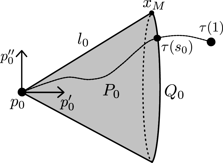
Figure 10: Cone spanned by the length $l_{0}$, the limit angle $\bar{\mathbf{\theta}}$ and the position of $s$. Every function from $\mathcal{F}_{\kappa_{0}}$ will necessarily leave $P_{0}$ by crossing $Q_{0}$ at $\tau(t_{0})$ to reach a point $\tau(1)$ outside $P_{0}$.

Proof.

Let us decompose the problem into two parts. First, let us show that all circles with center $(0,R)$ and radius $R\geq R_{0}$ will intersect $Q_{0}$. Second, let us show that all paths from $\mathcal{F}_{\kappa_{0}}$ will necessarily leave $P_{0}$ by crossing $Q_{0}$, such that there is no path crossing the ball $B_{R}(0,R)$ for given curvature $\kappa=\frac{1}{R}$.

• By construction the circle with radius $R_{0}$ intersects $Q_{0}$ at the point specified by angle $\bar{\mathbf{\theta}}=\theta(R)=\operatorname{asin}\left(\dfrac{l_{0}}{2R}\right)$. Since $\operatorname{asin}$ is monotone increasing on $[0,1]$, $l_{0},R\geq 0$ and $l_{0}\leq 2R$, we have that $\theta(R)\geq 0$. We have $\bar{\mathbf{\theta}}\geq\theta(R)$ since $\operatorname{asin}\left(\dfrac{l_{0}}{2R_{0}}\right)\geq\operatorname{asin}\left(\dfrac{l_{0}}{2R}\right)$ and therefore we can write $\dfrac{l_{0}}{2R_{0}}\geq\dfrac{l_{0}}{2R}$ since $\operatorname{asin}$ is monotone increasing. It follows that $R\geq R_{0}$.

• Let us define the left side of $p_{0}$ as $LD(p_{0})=\{(x_{0},x_{1})\in\mathbb{R}^{2}|(x_{0}-p_{0,0})\geq 0,(x_{1}-p_{0,1})\geq 0\}$ and let us construct a polygonal chain as defined by [14]. For a given $R\geq R_{0}$ start on the boundary of $P_{0}$ at point $p_{0}$ and follow direction $p_{0}^{\prime}$ until $Q_{0}$ is reached. At $Q_{0}$ move along on $Q_{0}$ until the ball with radius $R$ is intersected. This constitutes a polygonal forward chain [14]. This chain follows the boundary of $P_{0}\cap LD(p_{0})$. Let us apply Lemma $6$ in [14], stating that if a forward chain intersects the circle of radius $R$, then the reachable region of all paths in $\mathcal{F}_{\kappa_{0}}$ is given by $P_{0}\cap LD(p_{0})\setminus B_{R}(0,R)$. See Fig. 9 for visualization. Applying the pocket lemma from [41] it follows that no path can escape the region $P_{0}\cap LD(p_{0})\setminus B_{R}(0,R)$ except through $Q_{0}$ or the lower boundary. The same arguments apply for the right side of $p_{0}$ with $RD(p_{0})=\{x\in\mathbb{R}^{2}|x_{0}-p_{0,0}\geq 0,x_{1}-p_{0,1}\leq 0\}$ and therefore any function in $\mathcal{F}_{\kappa_{0}}$ starting in $p_{0}$ can escape the region $P_{0}\setminus(B_{R}(0,R)\cup B_{R}(0,-R))\subset P_{0}$ only through the arc segment $Q_{0}$. Since $\tau(1)\notin P_{0}$, the result follows.

∎

Theorem 4 assures that a particle starting at $(p_{0},p^{\prime}_{0})$, following $\tau\in\mathcal{F}_{\kappa_{0}}$ will always cross the arc segment $Q_{0}$. Now we consider the sweeping of disks $D_{\delta}(p)=\{x\in\mathbb{R}^{2}|\|x-p\|\leq\delta\}$ with radius $\delta$ along a path $\tau\in\mathcal{F}_{\kappa_{0}}$. Let us define $L_{0}=D_{\delta_{0}}(p_{0})$, $L_{1}(\theta)=D_{\delta_{1}}(p_{1}(\theta))$ with $p_{1}(\theta)=(l_{0}\cos(\theta),l_{0}\sin(\theta))$. Let $\oplus$ denote the Minkowski sum.

Theorem 5.

Let $L_{0}=D_{\delta_{0}}(p_{0})$. Then there exist a $\theta_{1}\in[-\bar{\mathbf{\theta}},\bar{\mathbf{\theta}}]$ with the property that for all $\tau\in\mathcal{F}_{\kappa_{0}}$ there exists $s_{0}\in[0,1]$ such that $L_{1}(\theta_{1})\subset(\tau(s_{0})\oplus L_{0})$ if $\delta_{1}\leq\delta_{0}$.

Proof.

Applying Theorem 4 a function $\tau\in\mathcal{F}_{\kappa_{0}}$ will necessarily intersect $Q_{0}$. Let $\tau(s_{0})\in Q_{0}$ be the intersection point. Let us choose $p_{1}(\theta_{1})=\tau(s_{0})$ as the position of link $L_{1}$. $\theta_{1}$ can be computed as $\theta_{1}=\operatorname{acos}\left(\dfrac{(\tau(s_{0})-\tau(0))^{T}p_{0}^{\prime}}{l_{0}}\right)$. The volume of link $L_{1}(\theta_{1})$ is given by $(\tau(s_{0})\oplus L_{1}(\theta_{1}))$, and is smaller than $(\tau(s_{0})\oplus L_{0})$ exactly when $\delta_{1}\leq\delta_{0}$.

∎

A.2 Multi Link Chain

Let $L_{0},\cdots,L_{N}\in D^{2}$ be disk links of radius $\delta_{0},\cdots,\delta_{N}$ connected by lines of equal length $l_{0},\cdots,l_{N-1}$ with $l_{0}=\cdots=l_{N-1}$, $\delta_{i}>0$, $l_{i}>\delta_{i}+\delta_{i+1}$ (no overlapping disks), $\delta_{i}\leq\delta_{0}$ for all $i>0$ and joint limits $\{\{-\bar{\mathbf{\theta}}_{0},\bar{\mathbf{\theta}}_{0}\},\cdots,\{-\bar{\mathbf{\theta}}_{N-1},\bar{\mathbf{\theta}}_{N-1}\}\}$ with $\bar{\mathbf{\theta}}_{0}=\cdots=\bar{\mathbf{\theta}}_{N-1}$. We will refer to this serial kinematic chain structure as $\mathcal{R}_{L}^{N}$.

Let $V(\theta_{0},\cdots,\theta_{N-1})$ be the swept volume of the chain without the links for a given set of configurations. We define $P_{N}$ as the union of all swept volumes of the chain under the constraint that $-\bar{\mathbf{\theta}}\leq\theta_{i}\leq\bar{\mathbf{\theta}}$ for every $i\in[0,N-1]$. This is depicted in Fig. 11. Further, let $Q_{N}$ be the part of the outer border which we obtain by removing the swept volume of the minimum joint configuration $V(\theta_{0}=-\bar{\mathbf{\theta}},\cdots,\theta_{N-1}=-\bar{\mathbf{\theta}})$, and the swept volume of the maximum joint configuration $V(\theta_{0}=-\bar{\mathbf{\theta}},\cdots,\theta_{N-1}=-\bar{\mathbf{\theta}})$, from the boundary of $P_{N}$. $Q_{N}$ is shown in Fig. 11.

As in the $N=1$ case, let us construct a functional space $\mathcal{F}_{\kappa_{N}}$ as

$$\mathcal{F}_{P_{N}} =\{\tau\in\Phi_{2}\ |\ \tau(0)=p_{0},\tau^{\prime}(0)=p_{0}^{\prime},\tau(1)\notin P_{N}\}$$ (16)

Let $\mathcal{F}_{\kappa_{N}}\subseteq\mathcal{F}_{P_{N}}$ be the subspace of curvature constrained functions

$$\mathcal{F}_{\kappa_{N}} =\{\tau\in\mathcal{F}_{P_{N}}\ |\ \kappa(\tau(s))\leq\kappa_{N}\}$$ (17)

$$\kappa_{N} =\frac{2\sin(\bar{\mathbf{\theta}})}{Nl_{0}},N>1$$ (18)

Figure 11: A succession of cones, spanning the space between $s$ and $Q_{N}$, which necessarily has to be traversed by any function from $\mathcal{F}_{\kappa_{N}}$.

For $N=1$, we proved that there exist $\theta_{0}$ such that $L_{1}(\theta_{0})\in\tau\oplus L_{0}(p_{0})$. For $N>1$, we need to take into account the change of orientation when the point has moved from $L_{0}$ to $L_{1}$. At $L_{1}$, we need to make sure that the obtained orientation $\theta_{0}$ and the next orientation $\theta_{1}$ are both below the maximum orientation $\bar{\mathbf{\theta}}$. See Fig. 12 for clarification.

To ensure that we can always find a feasible configuration, such that all links are on $\tau$, we therefore need to ensure that $\theta_{i}+\theta_{i-1}\leq\bar{\mathbf{\theta}}$ for all $i\in[1,N]$.

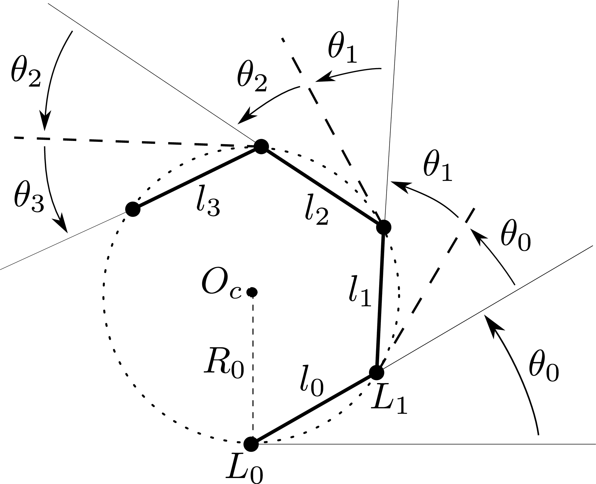
Figure 12: Serial kinematic chain along a curve $\tau$ with constant curvature $\kappa_{N}$.

We like to rewrite all angles in terms of the radius of the osculating circle $R_{0}$ and the length of the links $l_{i}$. The angle $\theta_{i}$ can be readily expressed as

$$\theta_{i}(R_{0},l_{i}) =\arctan{\left(\dfrac{l_{i}}{\sqrt{4R_{0}^{2}-l_{i}^{2}}}\right)}$$ (19)

This expression is obtained by centering a coordinate system at the center $O_{c}=(0,0)$ of the circle, then drawing two circles, one about $O_{c}$ with radius $R_{0}$, one about $L_{1}$ with radius $l_{0}$. Since we have chosen $R_{0}$ such that $R_{0}>l_{0}$, those circles have two intersection points. The two intersection points together with $O_{c}$ and $L_{1}$ create a geometric kite, which can be analyzed by geometrical inspection to arrive at the equation, see circle-circle intersection .

Let

$$R_{0} =\dfrac{Nl_{0}}{2\sin{\bar{\mathbf{\theta}}}}$$ (20)

such that $\mathcal{F}_{\kappa_{N}}$ is defined by $\kappa_{N}=\frac{1}{R_{0}}$.

Lemma 1.

Given a path $\tau\in\mathcal{F}_{\kappa_{N}}$ with $\frac{1}{\kappa_{N}}=R_{0}=\dfrac{Nl_{0}}{2\sin{\bar{\mathbf{\theta}}}}$ and $N>1$, there exist joint configurations $\theta_{1},\cdots,\theta_{N}$ for the serial kinematic chain $\mathcal{R}_{L}^{N}$, such that every $L_{i}$ is located on $\tau$. Furthermore, the maximum distance between $\tau$ and the lines $(L_{0}L_{1})\cdots(L_{N-1}L_{N})$ is given by

$$d_{\kappa_{N}}=R_{0}-\sqrt{R_{0}^{2}-\dfrac{l_{0}^{2}}{4}}$$ (21)

Proof.

Evaluating $\theta_{i}$ at $R_{0}$ gives

$$\theta_{i}(R_{0},l_{0})=\theta_{i}(N)=\arctan{\left(\dfrac{\sin{\bar{\mathbf{\theta}}}}{\sqrt{N^{2}-\sin^{2}{\bar{\mathbf{\theta}}}}}\right)}$$ (22)

for $N>1$. By induction on $N$, we get for $N=2$

$$\theta_{i}(2) =\arctan{\left(\dfrac{\sin{\bar{\mathbf{\theta}}}}{\sqrt{4-\sin^{2}{\bar{\mathbf{\theta}}}}}\right)}\leq\arctan{\left(\dfrac{\sin{\bar{\mathbf{\theta}}}}{2}\right)}$$ (23)

$$\leq\dfrac{\sin{\bar{\mathbf{\theta}}}}{2}\leq\dfrac{\bar{\mathbf{\theta}}}{2}$$

whereby we relied on the fact that for $x>0$ we have $\arctan(x)\leq x$ since $\arctan^{\prime}(x)=\frac{1}{1+x^{2}}\leq 1$, for $x>0$ we have $\sin(x)\leq x$ since $\sin^{\prime}(x)=\cos(x)\leq 1$.

We now observe that

$$\theta_{i}(N) =\arctan{\left(\dfrac{\sin{\bar{\mathbf{\theta}}}}{\sqrt{N^{2}-\sin^{2}{\bar{\mathbf{\theta}}}}}\right)}\geq\arctan{\left(\dfrac{\sin{\bar{\mathbf{\theta}}}}{N}\right)}$$ (24)

$$\geq\arctan{\left(\dfrac{\sin{\bar{\mathbf{\theta}}}}{\sqrt{(N+1)^{2}-\sin^{2}{\bar{\mathbf{\theta}}}}}\right)}=\theta_{i}(N+1)$$

which shows that $\theta_{i}(N)+\theta_{i-1}(N)\geq\theta_{i}(N+1)+\theta_{i-1}(N+1)$. Therefore $\bar{\mathbf{\theta}}\geq\theta_{i}(2)+\theta_{i-1}(2)\geq\cdots\geq\theta_{i}(N)+\theta_{i-1}(N)$ for $N>1$ as required.

Given the constant maximum curvature $\kappa_{N}$, the points $L_{i},L_{i-1}$ and $O_{c}$ are creating an isosceles triangle. See Fig. 12 for clarification. The maximum distance $d_{i}$ of the line $(L_{i}L_{i-1})$ and the circle can therefore be obtained by subtracting the height of the isosceles triangle from the radius of the circle as $d_{\kappa_{N}}=R_{0}-\sqrt{R_{0}^{2}-\dfrac{l_{i}^{2}}{4}}$.

∎

The swept volume of the root link $L_{0}$ will be the Minkowski sum with the path $\tau$, i.e. $V_{L_{0}}(\tau)=L_{0}\oplus\tau$. However, the sublinks will not lie inside of this swept volume at the starting configuration. To circumvent this problem we imagine the path $\tau$ being extended along the positions of the sublinks at the start configuration.

We call this extended part $\tau_{I}\in\mathcal{F}_{\kappa_{N}}$. $\tau_{I}$ can be obtained by computing a path which starts at $s=0$ at the position of the sublink $L_{N}$ at the start configuration, and follows each sublink $L_{i}$ until it reaches $L_{0}$ at instance $s=1$, such that $\tau_{I}(1)=\tau(0)$ and $\dot{\tau}_{I}(1)=\dot{\tau}(0)$.

We claim that along $\tau_{I}\circ\tau_{\kappa_{N}}$ we can find at least one configuration of the sublinks, such that the volume of the sublinks is inside the swept volume of the root link.

Theorem 6.

Let $\tau=\tau_{I}\circ\tau_{\kappa_{N}}\in\mathcal{F}_{\kappa_{N}}$. If the root link $L_{0}$ moves along $\tau_{\kappa_{N}}$, then for $\delta_{i}\leq\delta_{0}$ and $d_{\kappa_{N}}\leq\delta_{0}$, we have that there exists at least one configuration $\theta_{1}(s),\cdots,\theta_{N}(s)$ for any $s\in[0,1]$ such that the volume of the serial kinematic chain $\mathcal{R}_{L}^{N}$ is a subset of $\tau\oplus L_{0}$

Proof.

By Theorem 1 $\theta_{1}(s),\cdots,\theta_{N}(s)$ can be chosen such that the center of every $L_{i}(\theta_{1}(s),\cdots,\theta_{i}(s))$ is located on $\tau$. Then there exists an instance $s_{i}\in[0,1]$ such that $L_{i}(\theta_{1}(s),\cdots,\theta_{i}(s))=\tau(s_{i})$. $L_{i}(\theta_{1}(s),\cdots,\theta_{i}(s))$ is a subset of $\tau\oplus L_{0}$ if $\delta_{0}\geq\delta_{i}$. By Lemma 1, the maximum distance of the serial kinematic chain at $\theta_{1}(s),\cdots,\theta_{N}(s)$ to $\tau$ is given by $d_{\kappa_{N}}$. If $\delta_{0}\geq d_{\kappa_{N}}$, then any point on the serial kinematic chain curve will be inside $\tau\oplus L_{0}$. ∎

References

- LaValle [2006] S. M. LaValle. Planning Algorithms. Cambridge University Press, 2006.
- Reif [1979] John H Reif. Complexity of the mover’s problem and generalizations. In Conference on Foundations of Computer Science, pages 421–427, 1979.
- Dalibard and Laumond [2011] Sébastien Dalibard and Jean-Paul Laumond. Linear Dimensionality Reduction in Random Motion Planning. International Journal of Robotics Research, 2011.
- Allen et al. [2014] PeterK. Allen, Matei Ciocarlie, and Corey Goldfeder. Grasp planning using low dimensional subspaces. In Ravi Balasubramanian and Veronica J. Santos, editors, The Human Hand as an Inspiration for Robot Hand Development, Springer Tracts in Advanced Robotics. Springer International Publishing, 2014.
- Zhang et al. [2009] Liangjun Zhang, Jia Pan, and Dinesh Manocha. Motion planning of human-like robots using constrained coordination. In IEEE International Conference on Humanoid Robots, 2009.
- Orthey et al. [2015] Andreas Orthey, Florent Lamiraux, and Olivier Stasse. Motion Planning and Irreducible Trajectories. In IEEE International Conference on Robotics and Automation, 2015.
- Himmelstein et al. [2010] Jesse C Himmelstein, Etienne Ferre, and J-P Laumond. Swept volume approximation of polygon soups. IEEE Transactions on Automation Science and Engineering, 2010.
- Ciocarlie et al. [2007] M. Ciocarlie, C. Goldfeder, and P. Allen. Dimensionality reduction for hand-independent dexterous robotic grasping. In IEEE International Conference on Intelligent Robots and Systems, 2007.
- Mahoney et al. [2010] Arthur Mahoney, Joshua Bross, and David Johnson. Deformable robot motion planning in a reduced-dimension configuration space. In IEEE International Conference on Robotics and Automation, 2010.
- Kabul et al. [2007] Ilknur Kabul, Russell Gayle, and Ming C Lin. Cable route planning in complex environments using constrained sampling. In ACM Symposium on Solid and Physical Modeling. ACM, 2007.
- Salzman et al. [2016] O. Salzman, K. Solovey, and D. Halperin. Motion planning for multilink robots by implicit configuration-space tiling. Robotics and Automation Letters, 1(2), July 2016.
- Bereg and Kirkpatrick [2005] Sergey Bereg and David Kirkpatrick. Curvature-bounded traversals of narrow corridors. In Symposium on Computational geometry. ACM, 2005.
- Banchoff and Lovett [2015] Thomas F Banchoff and Stephen T Lovett. Differential geometry of curves and surfaces. CRC Press, 2015.
- Ahn et al. [2012] Hee-Kap Ahn, Otfried Cheong, Jiří Matoušek, and Antoine Vigneron. Reachability by paths of bounded curvature in a convex polygon. Computational Geometry, 2012.
- Guha and Tran [2005] Sumanta Guha and Son Dinh Tran. Reconstructing curves without delaunay computation. Algorithmica, 2005.
- Hirose and Yamada [2009] Shigeo Hirose and Hiroya Yamada. Snake-like robots [Tutorial]. Robotics and Automation Magazine, 2009.
- Conkur and Gurbuz [2008] Erdinc Sahin Conkur and Riza Gurbuz. Path Planning Algorithm for Snake–Like Robots. Information Technology And Control, 2008.
- Liu et al. [2004] Jinguo Liu, Yuechao Wang, Bin Ii, and Shugen Ma. Path planning of a snake-like robot based on serpenoid curve and genetic algorithms. In Intelligent Control and Automation, 2004.
- Henning et al. [1998] W. Henning, F. Hickman, and Howie Choset. Motion Planning for Serpentine Robots. In Proceedings of ASCE Space and Robotics, 1998.
- Rollinson and Choset [2011] David Rollinson and Howie Choset. Virtual Chassis for Snake Robots. In IEEE International Conference on Intelligent Robots and Systems, 2011.
- Cappo and Choset [2014] E.A. Cappo and H. Choset. Planning end effector trajectories for a serially linked, floating-base robot with changing support polygon. In American Control Conference, 2014.
- Sfakiotakis et al. [2014] Michael Sfakiotakis, Asimina Kazakidi, Avgousta Chatzidaki, Theodoros Evdaimon, and Dimitris P Tsakiris. Multi-arm robotic swimming with octopus-inspired compliant web. In IEEE International Conference on Intelligent Robots and Systems, 2014.
- Cianchetti et al. [2015] M Cianchetti, M Calisti, L Margheri, M Kuba, and C Laschi. Bioinspired locomotion and grasping in water: the soft eight-arm octopus robot. Bioinspiration & Biomimetics, 2015.
- Calisti et al. [2015] Marcello Calisti, Francesco Corucci, Andrea Arienti, and Cecilia Laschi. Dynamics of underwater legged locomotion: modeling and experiments on an octopus-inspired robot. Bioinspiration & Biomimetics, 2015.
- Harada et al. [2010] Kensuke Harada, Eiichi Yoshida, and Kazuhito Yokoi, editors. Motion Planning for Humanoid Robots. Springer, 2010.
- Vahrenkamp et al. [2009] Niko Vahrenkamp, Dmitry Berenson, Tamim Asfour, James Kuffner, and Rüdiger Dillmann. Humanoid motion planning for dual-arm manipulation and re-grasping tasks. In IEEE International Conference on Intelligent Robots and Systems, 2009.
- Escande et al. [2013] Adrien Escande, Abderrahmane Kheddar, and Sylvain Miossec. Planning contact points for humanoid robots. Robotics and Autonomous Systems, 61(5):428 – 442, 2013. ISSN 0921-8890. doi: 10.1016/j.robot.2013.01.008.
- Hauser et al. [2008] Kris Hauser, Timothy Bretl, Kensuke Harada, and Jean-Claude Latombe. Using motion primitives in probabilistic sample-based planning for humanoid robots. In Algorithmic foundation of robotics VII, pages 507–522. Springer, 2008.
- Deits and Tedrake [2014] Robin Deits and Russ Tedrake. Footstep Planning on Uneven Terrain with Mixed-Integer Convex Optimization. In IEEE International Conference on Humanoid Robots, 2014.
- Zhang et al. [2014] Yajia Zhang, Jingru Luo, Kris Hauser, H Andy Park, Manas Paldhe, CS Lee, Robert Ellenberg, Brittany Killen, Paul Oh, Jun Ho Oh, et al. Motion planning and control of ladder climbing on DRC-Hubo for DARPA Robotics Challenge. In IEEE International Conference on Robotics and Automation, 2014.
- El Khoury et al. [2013] Antonio El Khoury, Florent Lamiraux, and Michel Taïx. Optimal motion planning for humanoid robots. In IEEE International Conference on Robotics and Automation, pages 3136–3141, 2013.
- Farber [2003] Michael Farber. Topological complexity of motion planning. Discrete and Computational Geometry, 29(2), 2003.
- Hatton and Choset [2011] Ross L Hatton and Howie Choset. Geometric motion planning: The local connection, stokes’ theorem, and the importance of coordinate choice. International Journal of Robotics Research, 30(8), 2011.
- Munkres [2000] James Munkres. Topology. Pearson, 2000.
- Bloch [2003] Anthony M Bloch. Nonholonomic Mechanics and Control. Interdisciplinary Applied Mathematics, volume 24. Springer New York, 2003.
- LaValle and Kuffner [2001] Steven M LaValle and James J Kuffner. Randomized kinodynamic planning. International Journal of Robotics Research, 2001.
- Ladd and Kavraki [2004] Andrew M Ladd and Lydia E Kavraki. Fast tree-based exploration of state space for robots with dynamics. In Algorithmic Foundations of Robotics VI. Springer, 2004.
- Şucan and Kavraki [2009] Ioan A Şucan and Lydia E Kavraki. Kinodynamic motion planning by interior-exterior cell exploration. In Algorithmic Foundation of Robotics VIII. Springer, 2009.
- Li et al. [2016] Yanbo Li, Zakary Littlefield, and Kostas E Bekris. Asymptotically optimal sampling-based kinodynamic planning. International Journal of Robotics Research, 2016.
- Karaman and Frazzoli [2011] Sertac Karaman and Emilio Frazzoli. Sampling-based algorithms for optimal motion planning. International Journal of Robotics Research, 30(7), 2011.
- Agarwal et al. [2002] Pankaj K Agarwal, Therese Biedl, Sylvain Lazard, Steve Robbins, Subhash Suri, and Sue Whitesides. Curvature-constrained shortest paths in a convex polygon. SIAM Journal on Computing, 2002.