A Hybrid Universal Blind Quantum Computation

Abstract

In blind quantum computation (BQC), a client delegates her quantum computation to a server with universal quantum computers who learns nothing about the client’s private information. In measurement-based BQC model, entangled states are generally used to realize quantum computing. However, to generate a large-scale entangled state in experiment becomes a challenge issue. In circuit-based BQC model, single-qubit gates can be realized precisely, but entangled gates are probabilistically successful. This remains a challenge to realize entangled gates with a deterministic method in some systems. To solve above two problems, we propose the first hybrid universal BQC protocol based on measurements and circuits, where the client prepares single-qubit states and the server performs universal quantum computing. We analyze and prove the correctness, blindness and verifiability of the proposed protocol.

I Introduction

Recently, blind quantum computation (BQC) becomes a hot topic in quantum information processing since it can be applied to realize clients’ private quantum computing. In BQC, measurement-based model and circuit-based model have been studied for years 1Broadbent09 ; Barz12 ; 2Morimae13 ; qian17 ; 3Li14 ; 4Sheng15 ; 5Morimae2012 ; 8Morimae2015 ; Yu18 ; Childs2005 ; 22Fisher2014 ; Broa15 ; Mar16 ; Walther ; xiao18 . A. Broadbent et al. 1Broadbent09 in 2009 firstly implemented a universal BQC protocol by measuring an $m\times n$ dimensional blind brickwork state, which is called Broadbent-Fitzsimons-Kashefi (BFK) protocol. In BFK protocol, the client can prepare single-qubit states $\{|\pm_{\theta}\rangle=\frac{1}{\sqrt{2}}(|0\rangle+e^{i\theta}|1\rangle)|\ \theta=0,\frac{\pi}{4},\frac{2\pi}{4},\ldots,\frac{7\pi}{4}\}$. Based on BFK protocol, multi-server BQC protocols were proposed in 2Morimae13 ; 3Li14 ; 4Sheng15 . A BQC protocol for single-qubit gates X, Y, T, Z has been realized by measuring blind topological states, where the error threshold is explicitly calculated 5Morimae2012 . A universal BQC protocol based on Affleck-Kennedy-Lieb-Tasaki (AKLT) states has been implemented, where the universal gates set consists of blind Z-rotation, blind X-rotation and controlled-Z followed by blind Z-rotations 8Morimae2015 . In experiments, S. Barz et al. Barz12 realized a demonstration for the privacy of quantum inputs, computations, and outputs. Furthermore, the verifiable BQC protocols and other interesting BQC protocols have been proposed 7Morimae2014 ; 6Hayashi2015 ; Gheor15 ; Fit15 ; Fu16 ; Moe16 ; Anne17 ; 1Gio13 ; 13Sun15 ; 14Greg16 ; 16Delg15 ; 25Hua ; 30Huang . In 13Sun15 , a blind quantum computing about symmetrically private retrieval was proposed, where a client Alice has limited quantum technologies and queries a item of the database owned by a server Bob who has a fledged quantum computer. In the protocol, the privacy of both participants can be preserved: Bob knows nothing about what Alice has retrieved, and Alice can only get the information that she wants to query of the database, where the related private retrieval schemes can refer to Gao15 ; Gao16 ; Wei18 .

For quantum computers, it is important to prepare entangled states that can be applied to quantum computing Rausse01 , quantum simulation Seth96 and so on. In measurement-based BQC model, the key problem is how to generate large-scale entangled states 1Broadbent09 ; Horodecki09 in space-separated and individual-controllable quantum systems such as the brickwork state 1Broadbent09 , AKLT state 8Morimae2015 . In experiments, great progress has been made in preparing multi-qubit entangled states. The number of qubits in an entangled state Friis18 reaches to 20 in trapped-ion system, while the number is 10 both in superconducting Song17 and photonic systems Lin16 . It is difficult to describe a large-scale entangled state since the dimension of Hilbert space is exponentially increasing. In circuit-based BQC model Childs2005 ; 22Fisher2014 ; Broa15 ; Mar16 ; Walther , the entangled gates are realized probabilistically such as the successful probability in optical system is $1/16$ in Koashi01 , $1/9$ in Ralph02 , $1/4$ in Pittman01 , $1/3$ in Hofmann02 and $21/25$ in Brien03 .

In this paper, we first propose a hybrid universal BQC protocol (HUBQC), which is based on measurements and circuits. Intuitively, we make full use of advantages of two models. Specially, entangled gates can be realized with a deterministic method in measurement-based model, solving the probabilistic realization of entangled gates problem in circuit-based model. Meanwhile, the single-qubit gates can also be realized without too many qubits in circuit-based model, solving experimentally generation of a large-scale entangled state problem in measurement-based model. A client Alice generates initial states and a server Bob performs operations and measurements. The entangled gates can be realized by measuring graph states and single-qubit gates can be operated on the suitable qubits with an predefined order. We not only prove the correctness and blindness of the protocol but also have verifiability which implies to verify Bob’s honesty and the correctness of measurement outcomes. Finally, we apply HUBQC protocol to realize blind quantum Fourier transform. For blindness, measurement process has adopted the encryption algorithm from BFK protocol.

The rest of this paper is organized as follows. We present the preliminaries in Section II. The definition and structure of the graph state $|Cluster\rangle$ are presented in Section III. The universal blind quantum computation protocol is in Section IV. We show the analyses and proofs of correctness, blindness and verifiability as well as a application of our protocol in Section V. At last, our discussions and conclusions are given in Section VI.

II Preliminaries

II.1 Basic principles of circuit-based quantum computation

In 2000MAN , it points out that an arbitrary unitary operator U can be decomposed into the combinations of rotation operators. We first give the rotation operators as follows:

$$\begin{array}[]{l}\displaystyle R_{x}(\alpha)=\left(\begin{array}[]{cc}cos\frac{\alpha}{2}&-isin\frac{\alpha}{2}\\ -isin\frac{\alpha}{2}&cos\frac{\alpha}{2}\\ \end{array}\right),\\ \displaystyle R_{y}(\beta)=\left(\begin{array}[]{cc}cos\frac{\beta}{2}&-sin\frac{\beta}{2}\\ sin\frac{\beta}{2}&cos\frac{\beta}{2}\\ \end{array}\right),\\ \displaystyle R_{z}(\gamma)=\left(\begin{array}[]{cc}e^{\frac{-i\gamma}{2}}&0\\ 0&e^{\frac{i\gamma}{2}}\\ \end{array}\right),\end{array}$$ (10)

where $\alpha,\beta,\gamma\in[0,2\pi]$. Particularly, if the rotation angle is $\pi$ about $x$-axis, $y$-axis and $z$-axis respectively, we get

$$R_{x}(\pi)=iX,\ R_{y}(\pi)=XZ,\ R_{z}(\pi)=-iZ.$$ (11)

If there exist $\theta$, $\alpha$, $\beta$ and $\gamma$, s.t. an arbitrary unitary operator U has the decompositions as follows:

$$\begin{array}[]{l}\displaystyle U=e^{i\theta}R_{z}(\alpha)R_{y}(\beta)R_{z}(\gamma)\\ \displaystyle\qquad\qquad=\left(\begin{array}[]{cc}e^{i(\theta-\frac{\alpha}{2}-\frac{\gamma}{2})}cos\frac{\beta}{2}&-e^{i(\theta-\frac{\alpha}{2}+\frac{\gamma}{2})}sin\frac{\beta}{2}\\ e^{i(\theta+\frac{\alpha}{2}-\frac{\gamma}{2})}sin\frac{\beta}{2}&e^{i(\theta+\frac{\alpha}{2}+\frac{\gamma}{2})}cos\frac{\beta}{2}\\ \end{array}\right),\\ \displaystyle U=e^{i\theta}R_{z}(\alpha)R_{x}(\beta)R_{z}(\gamma)\\ \displaystyle\qquad\qquad=\left(\begin{array}[]{cc}e^{i(\theta-\frac{\alpha}{2}-\frac{\gamma}{2})}cos\frac{\beta}{2}&-ie^{i(\theta-\frac{\alpha}{2}+\frac{\gamma}{2})}sin\frac{\beta}{2}\\ -ie^{i(\theta+\frac{\alpha}{2}-\frac{\gamma}{2})}sin\frac{\beta}{2}&e^{i(\theta+\frac{\alpha}{2}+\frac{\gamma}{2})}cos\frac{\beta}{2}\\ \end{array}\right),\\ \displaystyle U=e^{i\theta}R_{y}(\alpha)R_{x}(\beta)R_{y}(\gamma)=e^{i\theta}\cdot\\ \displaystyle\left(\begin{array}[]{cc}cos\frac{\beta}{2}cos\frac{\alpha+\gamma}{2}+isin\frac{\beta}{2}sin\frac{\alpha-\gamma}{2}&-cos\frac{\beta}{2}sin\frac{\alpha+\gamma}{2}-isin\frac{\beta}{2}cos\frac{\alpha-\gamma}{2}\\ cos\frac{\beta}{2}sin\frac{\alpha+\gamma}{2}-isin\frac{\beta}{2}cos\frac{\alpha-\gamma}{2}&cos\frac{\beta}{2}cos\frac{\alpha+\gamma}{2}-isin\frac{\beta}{2}sin\frac{\alpha-\gamma}{2}\\ \end{array}\right).\end{array}$$ (24)

Here, we only show three decomposition forms, the other three decompositions $y\textnormal{-}z\textnormal{-}y$, $x\textnormal{-}z\textnormal{-}x$, $x\textnormal{-}y\textnormal{-}x$ are similar. Next, we give the $z\textnormal{-}y\textnormal{-}z$ decomposition for gates H, S, Z, T, X, Y as follows:

$$\begin{array}[]{l}\displaystyle H=e^{\frac{i\pi}{2}}R_{y}(\frac{\pi}{2})R_{z}(\pi),\ S=e^{\frac{i\pi}{4}}R_{z}(\frac{\pi}{2}),\ Z=e^{\frac{i\pi}{2}}R_{z}(\pi),\\ \displaystyle X=e^{\frac{i\pi}{2}}R_{y}(\pi)R_{z}(\pi),\ T=e^{\frac{i\pi}{8}}R_{z}(\frac{\pi}{4}),\ Y=e^{\frac{i\pi}{2}}R_{y}(\pi),\end{array}$$ (27)

For the $z\textnormal{-}x\textnormal{-}z$ decomposition of rotation operators of above gates, we obtain

$$\begin{array}[]{l}\displaystyle S=e^{\frac{i\pi}{4}}R_{z}(\frac{\pi}{2}),\quad Z=e^{\frac{i\pi}{2}}R_{z}(\pi),\quad T=e^{\frac{i\pi}{8}}R_{z}(\frac{\pi}{4}),\\ \displaystyle X=e^{\frac{i\pi}{2}}R_{x}(\pi),\quad Y=e^{\frac{i\pi}{2}}R_{x}(\pi)R_{z}(\pi),\\ \displaystyle H=e^{\frac{i\pi}{2}}R_{z}(\frac{\pi}{2})R_{x}(\frac{\pi}{2})R_{z}(\frac{\pi}{2}).\end{array}$$ (31)

For the $y\textnormal{-}x\textnormal{-}y$ decomposition of rotation operators of above gates, we get

$$\begin{array}[]{l}\displaystyle S=e^{\frac{i\pi}{4}}R_{y}(\frac{-\pi}{2})R_{x}(\frac{\pi}{2})R_{y}(\frac{\pi}{2}),\ H=e^{\frac{i\pi}{2}}R_{x}(\pi)R_{y}(\frac{\pi}{2}),\\ \displaystyle Z=e^{\frac{i\pi}{2}}R_{y}(\frac{-\pi}{2})R_{x}(\pi)R_{y}(\frac{\pi}{2}),\ \ X=e^{\frac{i\pi}{2}}R_{x}(\pi),\\ \displaystyle T=e^{\frac{i\pi}{8}}R_{y}(\frac{-\pi}{2})R_{x}(\frac{\pi}{4})R_{y}(\frac{\pi}{2}),\ Y=e^{\frac{i\pi}{2}}R_{y}(\pi).\end{array}$$ (35)

Unexpected Pauli operators will appear in the process of circuit-based computation, therefore some main propagation relationships between rotation operators and Pauli operators can be expressed as follows:

$$\begin{array}[]{l}\displaystyle R_{x}(\beta)X=XR_{x}(\beta),\ \ \ R_{x}(\beta)Z=ZR_{x}(-\beta),\\ \displaystyle R_{y}(\beta)X=XR_{y}(-\beta),\ R_{y}(\beta)Z=ZR_{y}(-\beta),\\ \displaystyle R_{z}(\beta)X=XR_{z}(-\beta),\ R_{z}(\beta)Z=ZR_{z}(\beta).\end{array}$$ (39)

Besides, the relationship of the rotation angles is $R_{\phi}(\alpha+\beta)=R_{\phi}(\alpha)\cdot R_{\phi}(\beta)$, where $\phi\in\{x,y,z\}$.

II.2 Basic principles of measurement-based quantum computation

In this section, we introduce the principles of measurement-based quantum computation.

In the paper 1Broadbent09 , we first get the detailed definitions and technologies of single-qubit initial states, orthogonal projections measurements, gates corrections and two-qubit entanglement operators in measurement based quantum computation model. Second, if the measured qubits are not in the final column (vertical direction), the correction operations $X$, $Z$ and $R_{z}(\cdot)$ can be naturally absorbed by performing the adaptive projective measurements. Third, we also obtain the commutation relationships of Controlled-Z (CZ) with X, Z, $R_{z}(\cdot)$ in 1Broadbent09 . The three points also can be found in Danos07 ; Jozsa05 . In addition, the commutation relationships of Pauli operators with $R_{x}(\cdot)$, $R_{z}(\cdot)$ are found in Eq.(7). After measuring the former qubit in a large graph state, the following gate will act on the latter qubit: $W(\theta)=\frac{1}{\sqrt{2}}\left(\begin{array}[]{cc}1&e^{i\theta}\\ 1&-e^{i\theta}\\ \end{array}\right)=H\cdot P(\theta)$, where $P(\theta)=\left(\begin{array}[]{cc}1&0\\ 0&e^{i\theta}\\ \end{array}\right).$

III The definition and structure of the graph state $|Cluster\rangle$

Definition—In FIG. 1, we show the structure of an $m\times n$ dimensional entangled state $|Cluster\rangle$, where these single-qubit states in the state $|Cluster\rangle$ are $|\pm_{\omega_{j}}\rangle=\frac{1}{\sqrt{2}}(|0\rangle\pm e^{i\omega_{j}}|1\rangle)$ ($\omega_{j}=0,\frac{\pi}{4},\ldots,\frac{7\pi}{4}$). Suppose $m$ denote the horizontal rows and $n$ denote the vertical columns. The physical qubits are labelled as index $(a,b)$, where $a$ represents the $a$-th row and $b$ represents the $b$-th column.

1. For odd rows $a$ and columns $b\equiv 1$ (mod 6), applying operations CZ on qubits $(a,b)$ and $(a+1,b)$, $(a,b+2)$ and $(a+1,b+2)$.

2. For even rows $a$ and columns $b\equiv 4$ (mod 6), applying operations CZ on qubits $(a,b)$ and $(a+1,b)$, $(a,b+2)$ and $(a+1,b+2)$.

3. For each row $a$, applying operations CZ on qubits $(a,b)$ and $(a,b+1)$ where $1\leqslant a\leqslant m,1\leqslant b\leqslant n$.

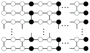
Figure 1: Schematic structure of a graph state $|Cluster\rangle$, where the black dots can be viewed as the outputs in former computing meanwhile the inputs in the latter computing. All white dots are auxiliary qubits to help complete the computing.

It can be seen from FIG. 1 that every unit state is an eight-qubit cluster state (See FIG. 2(1)) which can be used to realize entangled gates Controlled-NOT (CNOT) (See FIG. 2(2)).

IV A hybrid universal BQC protocol

Our HUBQC Protocol—The concrete steps of our protocol are as follows (See FIG. 3), where the client Alice has the ability to prepare the initial states and the server Bob can perform universal quantum computing without extracting Alice’s any private information.

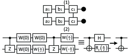
Figure 2: Schematic structure of an eight-qubit cluster state which refers to our previous work Xiao , where qubits labelled by $a_{f},b_{f},c_{f}$ ($f=1,2$) need to be measured. Except for a global phase factor, $W(\theta)$ is the same as $HR_{z}(\theta)$.

Step 1. Alice prepares all single-qubit states $|\pm_{\omega_{j}}\rangle$, $|0\rangle$, $|1\rangle$, $|\pm_{\mu_{j}}\rangle$ and sends them to Bob, where $\omega_{j},\mu_{j}\in\{0,\frac{\pi}{4},\cdots,\frac{7\pi}{4}\}$. These states $|\pm_{\omega_{j}}\rangle$ are used for computing and $|0\rangle$, $|1\rangle$, $|\pm_{\mu_{j}}\rangle$ are trap qubits. The reason choosing $|0\rangle$, $|1\rangle$, $|\pm_{\mu_{j}}\rangle$ as trap qubits is that $|0\rangle$, $|1\rangle$ are not entangled with $|\pm_{\mu_{j}}\rangle$ after performing CZ gates. While states $|\pm_{\mu_{j}}\rangle$ can be entangled with each other at most three qubits as long as they are in the suitable places. Note that, the connections with the states $|\pm_{\omega_{j}}\rangle$ are $|0\rangle$ and $|1\rangle$.

Step 2. Alice asks Bob to perform CZ gates to get eight-qubit cluster states and implement the corresponding measurements until Bob gets a graph state $|C\rangle$ (See Fig. 4). In Fig. 4, some qubits connected by dotted lines are trap qubits $|0\rangle$, $|1\rangle$, $|\pm_{\mu_{j}}\rangle$ and the others are computational qubits $|\pm_{{}_{j}}\rangle$. These trap qubits can be randomly attached to the $|Cluster\rangle$ state as long as they keep the structural consistency and do not affect the original computing.

Step 3. In Alice’s target algorithms, if single-qubit gates are required to implement first, Alice asks Bob to perform the above process in FIG. 3, where H and T are the combination of rotation operators. Bob first performs encrypted rotation operations on two black dots in the cluster state, where the encrypted rotation angles are $\xi_{j}=\nu_{j}+r_{j}\pi$ ($\nu_{j}$ is true rotation angles and $r_{j}$ is randomly chosen from $\{0,1\}$) and $R_{\phi}(\xi_{j})=R_{\phi}(r_{j}\pi+\nu_{j})=R_{\phi}(r_{j}\pi)R_{\phi}(\nu_{j})$ ($\phi\in\{x,y,z\}$). Note that, the encrypted angle $\xi_{j}$ and true rotation angles $\nu_{j}$ belong to the set $\{0,\frac{\pi}{4},\frac{2\pi}{4},\pi,\frac{5\pi}{4},\frac{6\pi}{4}\}$.

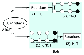
Figure 3: (Color online) Schematic diagram of our BQC protocol, where rotations denote the decompositions of gates H, T. The eight-qubit cluster state for realizing a CNOT gate belongs to state $|Cluster\rangle$.

Next, Bob measures every white dot qubit in the cluster state to get the CNOT gate, where the corresponding measurement angles are $\delta_{t}=\omega^{\prime}_{t}+\kappa_{t}+r_{t}\pi$ which belongs to the set $\{0,\frac{\pi}{4},\cdots,\frac{7\pi}{4}\}$. $r_{t}$ is randomly chosen from the set $\in\{0,1\}$, and $\omega^{\prime}_{t}=(-1)^{s_{t}^{X}}\omega_{t}+s^{Z}_{t}\pi$ depends on previous measurement outcomes. The measurement results are zero in the first row and the first column 1Broadbent09 .

Otherwise, Alice asks Bob to perform the below process in FIG. 3. Bob first measures the white dots qubits to get a CNOT gate and then performs rotation operators in black dots qubits to realize a single-qubit gate. Note that for gates CNOT, if the cluster states do not contain final quantum outputs in FIG. 4, the correction operations $R_{z}(\textnormal{-}\frac{\pi}{2})$ can be naturally absorbed by performing the projective measurements $|\pm_{\delta_{t}-\frac{\pi}{2}}\rangle$ since $|\pm_{\delta_{t}-\frac{\pi}{2}}\rangle$ is the same as $R_{z}(\textnormal{-}\frac{\pi}{2})|\pm_{\delta_{t}}\rangle=\frac{1}{\sqrt{2}}(e^{\frac{i\pi}{4}}|0\rangle\pm e^{i(\delta_{t}-\frac{\pi}{4})}|1\rangle)=\frac{e^{\frac{i\pi}{4}}}{\sqrt{2}}[|0\rangle\pm e^{i(\delta_{t}-\frac{\pi}{2})}|1\rangle]$ except for a global phase factor.

The above two processes can also be performed in trap qubits, therefore, Bob can not distinguish which are useful CNOT gates and trap gates CNOT in FIG. 4 to strengthened the security of our protocol.

Step 4. In the final quantum outputs, Alice asks Bob to perform the correct operations H and $R_{z}(\textnormal{-}\frac{\pi}{2})$. That is, Bob performs correct rotation operators $R_{x}(\cdot),R_{y}(\cdot)$ or $R_{z}(\cdot)$. After Bob returning all quantum outputs, Alice first measures the trap qubits to verify Bob’s honesty, where the number of trap qubits is optimal without having an impact on the computational efficiency. In fact, eight-qubits cluster states can also be used to realize single-qubit gates Xiao . Combined with trap gates and encoded measurement angles, it is impossible for Bob to know the position of CNOT gates.

In the protocol, Bob maybe implement Pauli attacks to change the original graph states. If Bob performs Pauli attacks X on $|0\rangle$, $|1\rangle$ or Z on $|\pm_{\mu_{j}}\rangle$ or XZ on $|0\rangle$, $|1\rangle$, $|\pm_{\mu_{j}}\rangle$, Alice will get violative results and she aborts the protocol. Note that, Alice knows all measurement results on traps with related basis. If Bob passes the verification, Alice will discard all traps and accept the results.

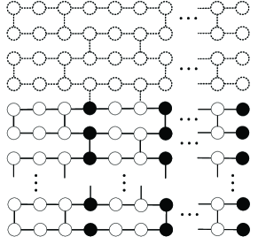
Figure 4: Schematic structure of an entangled state $|C\rangle$, where qubits connected by dotted lines are trap qubits $|0\rangle$, $|1\rangle$, $|\pm_{\mu_{j}}\rangle$ and solid lines are computational qubits $|\pm_{\omega_{j}}\rangle$. The positions of trap qubits are random without having an impact on the computing and keeping the structural consistency with computational qubits.

V Proofs and applications

We first prove the correctness, blindness and verifiability of our HUBQC protocol.

Correctness. All quantum outputs are correct when Bob performs the protocol honestly.

Proof: 1) In measurement-based process, the correctness of gate CNOT is showed in FIG. 5.

Since $H=e^{\frac{i\pi}{2}}R_{z}(\frac{\pi}{2})R_{x}(\frac{\pi}{2})R_{z}(\frac{\pi}{2})$ holds, we get $R_{z}(\textnormal{-}\frac{\pi}{2})H=e^{\frac{i\pi}{2}}R_{x}(\frac{\pi}{2})R_{z}(\frac{\pi}{2})$ in the below lines. After that, we obtain the circuit (1). And we get the circuit (2) via the relationship $HR_{z}(\alpha)H=R_{x}(\alpha)$. By correcting H and $R_{z}(\textnormal{-}\frac{\pi}{2})$, we receive the gate CNOT with the relationship $(R_{z}(\frac{\pi}{2})\otimes R_{x}(\frac{\pi}{2}))CZ(I\otimes R_{x}(\textnormal{-}\frac{\pi}{2}))CZ=CNOT$.

In the circuit process, the correctness can also be ensured since we have

$$\begin{array}[]{l}\displaystyle R_{x}(\nu_{j}+r\pi)=\begin{cases}R_{x}(\nu_{j}),&r=0\cr iXR_{x}(\nu_{j}),&r=1\end{cases},\\ \displaystyle R_{y}(\nu_{j}+r\pi)=\begin{cases}R_{y}(\nu_{j}),&r=0\cr XZR_{y}(\nu_{j}),&r=1\end{cases},\\ \displaystyle R_{z}(\nu_{j}+r\pi)=\begin{cases}R_{z}(\nu_{j}),&r=0\cr-iZR_{z}(\nu_{j}),&r=1\end{cases},\end{array}$$

where X, Z are commuted with rotation operations so they can be easily removed. $\square$

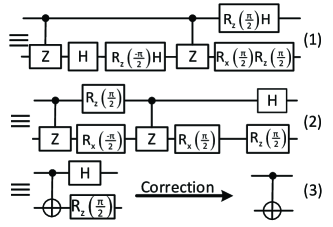
Figure 5: The simplification process of CNOT gate.

Blindness (quantum inputs). Suppose the quantum inputs are single-qubit states $|\pm_{\theta_{j}}\rangle$, $|0\rangle$, $|1\rangle$. Bob can not get anything from these qubits since the density matrices are maximally mixed from his point of view.

Proof: For single-qubit states $|\pm_{\theta_{j}}\rangle$ and $|0\rangle$, $|1\rangle$, where $\theta_{j}\in\{0,\frac{\pi}{4},\cdots,\frac{7\pi}{4}\}$, we have

$$\begin{array}[]{l}\displaystyle\frac{1}{18}[\sum\nolimits_{\theta_{j}}[|+_{\theta_{j}}\rangle\langle+_{\theta_{j}}|+|-_{\theta_{j}}\rangle\langle-_{\theta_{j}}|+|0\rangle\langle 0|+|1\rangle\langle 1|]\\ \displaystyle=\frac{1}{18}[|+\rangle\langle+|+|+_{\frac{\pi}{4}}\rangle\langle+_{\frac{\pi}{4}}|+\cdots+|+_{\frac{7\pi}{4}}\rangle\langle+_{\frac{7\pi}{4}}|\\ \displaystyle\qquad\ +|-\rangle\langle-|+|-_{\frac{\pi}{4}}\rangle\langle-_{\frac{\pi}{4}}|+\cdots+|-_{\frac{7\pi}{4}}\rangle\langle-_{\frac{7\pi}{4}}|\\ \displaystyle\qquad\ +|0\rangle\langle 0|+|1\rangle\langle 1|]=\frac{1}{2}I.\end{array}$$ (45)

From the equation, we can get the conclusion: the density matrix is independent of quantum inputs, that is, Bob get nothing from the initial states.$\square$

Blindness (graph states). The graph state $|C\rangle$ is completely blind including the dimension since it contains trap qubits.

Proof: Suppose the dimension of the graph state $|C\rangle$ is $m\times n$ known by Bob. However, the true dimension of state $|Cluster\rangle$ is smaller than $m\times n$. All units are eight-qubit cluster states, so nothing about the structure of state $|C\rangle$ is leaked. And the number and the positions of CNOT gates are secret for Bob. Moreover, all measurement angles are encrypted by one-time-pad. Therefore, Bob knows nothing about Alice’s quantum computing.$\square$

Blindness (algorithms and outputs). Here, two cases are considered: measurement-based process and circuit-based process. Bayes’ theorem can be used to prove the blindness of quantum algorithms and outputs: $\bf{a)}$ the conditional probability distribution of computational angles known by Bob is equal to its priori probability distribution, when Bob knows some classical information and measurement outcomes of any positive-operator valued measurements (POVMs) at any time; $\bf{b)}$ all quantum outputs are one-time padded to Bob.

Proof: In measurement-based process, the encrypted form is the same as the BFK protocol 1Broadbent09 , the blindness proofs of algorithms and outputs are also the same as those in 5Morimae2012 ; 8Morimae2015 . In circuit-based process, the encrypted form is $\xi_{j}=\nu_{j}+r\pi$, we give the blindness proofs of algorithms and outputs as follows.

We firstly analyse the effect of Bob’s rotation angles information $\Xi_{j}=\{\xi_{j}\}_{j=1}^{m}$ on Alice’s privacy 5Morimae2012 ; 8Morimae2015 . Suppose $V_{j}=\{\nu_{j}\}_{j=1}^{m}$, $R_{j}=\{r_{j}\}_{j=1}^{m}$, where $R_{j}\in\{0,1\}$ is a random variable chosen by Alice and $\{\Xi_{j},V_{j}\}\in S=\{\frac{k\pi}{4}\mid k=0,1,2,4,5,6\}$. Let $\Lambda\in\{1,\cdots,m\}$ be a random variable related with an operation. The conditional probability distribution of $\Xi_{j}$ given by $\Lambda=j$ and $V_{j}$ shows Bob’s knowledge which is about Alice’s rotation angles information. Based on Bayes’ theorem, we get

$$\begin{array}[]{l}\displaystyle p(\Xi_{j}=\{\xi_{j}\}_{j=1}^{m}\mid\Lambda=j,V_{j}=\{\nu_{j}\}_{j=1}^{m})\\ \displaystyle=\frac{p(\Lambda=j\mid\Xi_{j}=\{\xi_{j}\}_{j=1}^{m},V_{j}=\{\nu_{j}\}_{j=1}^{m})p(\Xi_{j}=\{\xi_{j}\}_{j=1}^{m},V_{j}=\{\theta_{j}\}_{j=1}^{m})}{p(\Lambda=j,V_{j}=\{\nu_{j}\}_{j=1}^{m})}\\ \displaystyle=\frac{p(\Lambda=j\mid\Xi_{j}=\{\xi_{j}\}_{j=1}^{m},V_{j}=\{\nu_{j}\}_{j=1}^{m})p(\Xi_{j}=\{\xi_{j}\}_{j=1}^{m})p(V_{j}=\{\nu_{j}\}_{j=1}^{m})}{p(\Lambda=j\mid V_{j}=\{\nu_{j}\}_{j=1}^{m})p(V_{j}=\{\nu_{j}\}_{j=1}^{m})}\\ \displaystyle=p(\Xi_{j}=\{\xi_{j}\}_{j=1}^{m})\cdot\frac{p(\Lambda=j\mid\Xi_{j}=\{\xi_{j}\}_{j=1}^{m},V_{j}=\{\nu_{j}\}_{j=1}^{m})}{p(\Lambda=j\mid V_{j}=\{\nu_{j}\}_{j=1}^{m})}\\ \displaystyle=p(\Xi_{j}=\{\xi_{j}\}_{j=1}^{m}).\end{array}$$

This implies that the conditional probability distribution of rotation angles known by Bob is equal to its priori probability distribution. So our HUBQC protocol satisfies the condition $\bf{a)}$.

Similarly, we can get the conditional probability as follows:

$$\begin{array}[]{l}\displaystyle p(R_{j}=\{r_{j}\}_{j=1}^{m}\mid\Lambda=j,\Xi_{j}=\{\xi_{j}\}_{j=1}^{m})\\ \displaystyle=\frac{p(\Lambda=j\mid R_{j}=\{r_{j}\}_{j=1}^{m},V_{j}=\{\nu_{j}\}_{j=1}^{m})p(R_{j}=\{r_{j}\}_{j=1}^{m},\Xi_{j}=\{\xi_{j}\}_{j=1}^{m})}{p(\Lambda=j,\Xi_{j}=\{\xi_{j}\}_{j=1}^{m})}\\ \displaystyle=\frac{p(\Lambda=j\mid R_{j}=\{r_{j}\}_{j=1}^{m},\Xi_{j}=\{\xi_{j}\}_{j=1}^{m})p(R_{j}=\{r_{j}\}_{j=1}^{m})p(\Xi_{j}=\{\xi_{j}\}_{j=1}^{m})}{p(\Lambda=j\mid V_{j}=\{\nu_{j}\}_{j=1}^{m})p(\Xi_{j}=\{\xi_{j}\}_{j=1}^{m})}\\ \displaystyle=p(R_{j}=\{r_{j}\}_{j=1}^{m})\frac{p(\Lambda=j\mid R_{j}=\{r_{j}\}_{j=1}^{m},\Xi_{j}=\{\xi_{j}\}_{j=1}^{m})}{p(\Lambda=j\mid\Xi_{j}=\{\xi_{j}\}_{j=1}^{m})}\\ \displaystyle=p(R_{j}=\{r_{j}\}_{j=1}^{m}).\end{array}$$

The result shows that the value $\{r_{j}\}_{j=1}^{m}$ is independent of $\Xi_{j}=\{\xi_{j}\}_{j=1}^{m}$, so our HUBQC protocol satisfies the condition $\bf{b)}$.$\square$

Verifiability. The verifiability is to ensure that the client Alice can obtain the correct results and the server Bob is honest. That is, if all measurements on traps show the correct results, the probability that a logical state of Alice’s computation is changed is exponentially small.

Proof: In our protocol, Alice adds some trap qubits around the state $|Cluster\rangle$. Bob knows neither the number of trap qubits nor their positions. When Bob returns these results, Alice makes a comparison between true results and Bob’s results on the trap qubits. If the error rate is acceptable, Alice accepts these results on computational qubits. Moreover, Alice can measure the quantum outputs traps, and then successfully verifies Bob’s honesty and the correctness of quantum computing.

Bob replaces the true $|C\rangle$ state with any states $\rho$. This equals to that Bob performs Pauli attacks I, X, Z, XZ. The proof is as follows, which refers to 7Morimae2014 .

Now we show that the probability that Alice is fooled by Bob is exponentially small. Since Bob might be dishonest, he will deviate from the correct steps. His general attack is a creation of a different state $\rho$ instead of $|C\rangle$. If he is honest, $\rho=|C\rangle\langle C|$. If he is not honest, $\rho$ can be any state. The case can be deduced to Pauli attacks by a completely positive-trace-preserving (CPTP) map, and the details can refer to 7Morimae2014 .

Suppose the qubits number of state $|C\rangle$ is $2N$, where the number of traps and computational qubits is $N$ respectively. Here, we denote that the number $N$ is optimal for traps. Then, the probability that all X operators of $\sigma_{\alpha}$ do not change any trap is $\frac{(2N-a)!\Pi_{k=0}^{a-1}(\frac{N}{2}-k)}{(2N)!}=(\frac{1}{2})^{a}\frac{\Pi_{k=0}^{a-1}(N-2k)}{\Pi_{k=0}^{a-1}(2N-k)}\leqslant(\frac{1}{2})^{a}\leqslant(\frac{1}{2})^{\alpha/3}$. We can obtain the same result for $max(a,b,c)=b$. For $max(a,b,c)=c$, we have $\frac{(2N-a)!\Pi_{k=0}^{a-1}(N-k)}{(2N)!}=\frac{\Pi_{k=0}^{a-1}(N-k)}{\Pi_{k=0}^{a-1}(2N-k)}\leqslant(\frac{1}{2})^{a}\leqslant(\frac{1}{2})^{\alpha/3}$. It implies that the probability that Alice is fooled by Bob is exponentially small. Hence our protocol is verifiable.$\square$

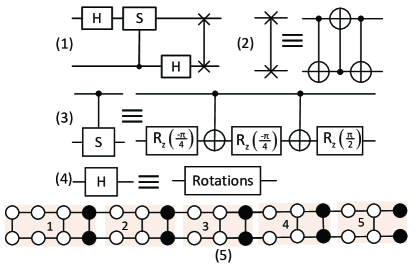
Figure 6: (Color online) (1) The quantum circuit is two-qubit QFT, where (2) shows the decomposition of SWAP gate, and (3) exhibits the decomposition of controlled-S, and (4) gives the combination of gate H, and (5) shows the structure of the graph state for realizing five CNOT gates, where trap qubits are not considered.

Application (Blind quantum Fourier transform)—With the help of our HUBQC protocol, we study the quantum Fourier transform (QFT) Marq10 ; Nam14 ; Lid17 and show the corresponding blind QFT protocol since multi-qubit QFT are the combinations of some single-qubit gates and entangled gates orderly.

We first explain how to realize blind two-qubit QFT. In FIG. 6, all gates can be decomposed into rotation operations and CNOT gates. In 2000MAN , the decomposition principle of every controlled unitary operator $U$ has been given. For the unitary operator $U$, there are unitary operators A, B, C such that $ABC=I$ and $U=e^{i\alpha}AXBXC$, where $\alpha$ is a global phase factor. Suppose $A=R_{z}(\beta)R_{y}(\frac{\gamma}{2}),B=R_{y}(\textnormal{-}\frac{\gamma}{2})R_{z}(\frac{\textnormal{-}(\delta+\beta)}{2}),C=R_{z}(\frac{(\delta-\beta)}{2})$, $U=S$, we have $\small S=e^{i\alpha}R_{z}(\beta)R_{y}(\gamma)R_{z}(\delta)=\left(\begin{array}[]{cc}1&0\\ 0&i\\ \end{array}\right)$. Set $\alpha=\frac{\pi}{4}$, $\beta=\frac{\pi}{2}$ and $\gamma=\delta=0$, so we get the Fig. 6(3) about the decomposition of controlled-S entangled gate.

We also give the multi-qubit QFT referred to 2000MAN and the corresponding blind QFT protocol also can be realized via a similar way, where gate controlled-$G_{n}$ can also be decomposed into a combination of rotation operations and CNOT gates. Let $U=G_{n}$, we have $\small U=\left(\begin{array}[]{cc}1&0\\ 0&e^{\frac{2\pi i}{2^{k}}}\\ \end{array}\right)$. We set $\alpha=\frac{\pi}{2^{k}}$, $\gamma=0$ and $\beta+\delta=\frac{2\pi}{2^{k}}$.

VI Discussions and Conclusions

In this section, we will discuss the measurement-based universal BQC , circuit-based universal BQC and our proposed HUBQC protocols.

$\bullet$ In measurement-based universal BQC model 1Broadbent09 , every gate needs ten-qubit cluster states. So it brings a challenge to generate multi-qubits entangled states in experiments. In our protocol, we can divide the universal BQC protocol into two processes: measurement-based process and circuit-based process. We do not need a large-scale entangled state since only entangled gate need to be realized by using cluster states.

$\bullet$ In circuit-based universal BQC model Koashi01 ; Ralph02 ; Pittman01 ; Hofmann02 ; Brien03 , entangled gates in some systems are probabilistically successful, while the cluster states can be to determinately realize entangled gates.

$\bullet$ In our HUBQC protocol, compared with other works 7Morimae2014 ; Moe16 , Alice has less workload since she only needs to measure trap qubits appearing in the final column of the graph state (See Fig. 4). In measurement-based process, $\omega^{\prime}_{t}+\kappa_{t}$ represents an actual measurement angle and $r_{t}$ is randomly chosen from $\{0,1\}$ in $\delta_{t}=\omega^{\prime}_{t}+\kappa_{t}+r_{t}\pi$. However, in circuit-based process, $r_{j}$ is also randomly chosen from $\{0,1\}$ such that $\xi_{j}$ can be mapped to a uniform distribution set. In both processes, quantum outputs are all encrypted.

In summary, we propose a universal blind quantum computation protocol based on measurements and circuits which only needs two participants: a client Alice and a server Bob. Alice prepares the initial states and sends to Bob who creates the entangled state. According to the computations, Alice asks Bob to perform single-qubit rotation operators or entangled gates. Since the graph state $|Cluster\rangle$ is surrounded by many traps, and the structure of traps is the same as that of computational qubits, the state $|C\rangle$ is blind from Bob’s perspective. In both measurement-based process and the circuit-based process, we encrypt the measurement angles and the rotation angles by one-time-pad. The correctness, blindness and verifiability have already been proved and the universality is obvious since the gates set is H, T, CNOT in our protocol.

References

- (1) A. Broadbent, J. Fitzsimons, E. Kashefi, Universal blind quantum computation, In Proceedings of the 50th Annual IEEE Symposium on Foundations of Computer Science, 2009, pp. 517–526.
- (2) S. Barz, E. Kashefi, A. Broadbent, J. F. Fitzsimons, A. Zeilinger, P. Walther, Demonstration of blind quantum computing, Science 335 (2012) 303–308.
- (3) T. Morimae, K. Fujii, Secure entanglement distillation for double-server blind quantum computation, Phys. Rev. Lett. 111 (2013) 020502.
- (4) X. Zhang, J. Weng, W. Lu, X. Li, W. Luo, X. Tan, Greenberger-horne-zeilinger states-based blind quantum computation with entanglement concentration, Sci. Rep. 7 (2017) 11104.
- (5) L. Qin, C. W. Hong, W. Chunhui, W. Zhonghua, Triple-server blind quantum computation using entanglement swapping, Phys. Rev. A 89 (2014) 040302.
- (6) Y.-B. Sheng, L. Zhou, Deterministic entanglement distillation for secure double-server blind quantum computation, Sci. Rep. 5 (2015) 7815.
- (7) T. Morimae, K. Fujii, Blind topological measurement-based quantum computation, Nat. Commun. 3 (2012) 1036.
- (8) T. Morimae, V. Dunjko, E. Kashefi, Ground state blind quantum computation on aklt states, Quantum Inf. Computat. 15 (2015) 200–234.
- (9) Y.-B. Sheng, L. Zhou, Blind quantum computation with noise environment, Phys. Rev. A 98 (2018) 052343.
- (10) A. M. Childs, Secure assisted quantum computation, Quantum inf. comput. 5 (2005) 456–466.
- (11) K. Fisher, A. Broadbent, L. Shalm, Z. Yan, J. Lavoie, R. Prevedel, T. Jennewein, K. Resch, Quantum computing on encrypted data, Nat. Commun. 5 (2014) 3074.
- (12) A. Broadbent, Delegating private quantum computations, Can. J. Phys. 93 (2015) 941–946.
- (13) K. Marshall, C. S. Jacobsen, C. Schfermeier, T. Gehring, C. Weedbrook, U. L. Andersen, Continuous-variable quantum computing on encrypted data, Nat. Commun. 7 (2016) 13794.
- (14) P. Walther, K. J. Resch, T. Rudolph, E. Schenck, H. Weinfurter, V. Vedral, M. Aspelmeyer, A. Zeilinger, Experimental one-way quantum computing, Nat. 434 (2005) 169–176.
- (15) X. Zhang, J. Weng, X. Li, W. Luo, X. Tan, T. Song, Single-server blind quantum computation with quantum circuit model, Quant. Inf. Process 17 (2018) 134.
- (16) T. Morimae, Verification for measurement-only blind quantum computing, Phys. Rev. A 89 (2014) 060302.
- (17) M. Hayashi, T. Morimae, Verifiable measurement-only blind quantum computing with stabilizer testing, Phys. Rev. Lett. 115 (2015) 220502.
- (18) A. Gheorghiu, E. Kashefi, P. Wallden, Robustness and device independence of verifiable blind quantum computing, New J. Phys. 17 (2015) 083040.
- (19) J. F. Fitzsimons, E. Kashefi, Unconditionally verifiable blind quantum computation, Phys. Rev. A 96 (2017) 012303.
- (20) K. Fujii, M. Hayashi, Verifiable fault tolerance in measurement-based quantum computation, Phys. Rev. A 96 (2017) 030301.
- (21) T. Morimae, Measurement-only verifiable blind quantum computing with quantum input verification, Phys. Rev. A 94 (2016) 042301.
- (22) A. Broadbent, How to verify a quantum computation, Theory of computing 14 (2018) 1–37.
- (23) V. Giovannetti, L. Maccone, T. Morimae, T. G. Rudolph, Efficient universal blind quantum computation, Phys. Rev. Lett. 111 (2013) 230501.
- (24) Z. Sun, J. Yu, P. Wang, L. Xu, Symmetrically private information retrieval based on blind quantum computing, Phys. Rev. A 91 (2015) 052303.
- (25) C. Greganti, M. C. Roehsner, S. Barz, T. Morimae, P. Walther, Demonstration of measurement-only blind quantum computing, New J. Phys. 18 (2016) 013020.
- (26) C. A. Pérez-Delgado, J. F. Fitzsimons, Iterated gate teleportation and blind quantum computation, Phys. Rev. Lett. 114 (2015) 220502.
- (27) H. L. Huang, W. S. Bao, T. Li, F. G. Li, X. Q. Fu, S. Zhang, H. L. Zhang, X. Wang, Universal blind quantum computation for hybrid system, Quantum Inf. Process. 16 (2017) 199.
- (28) H. L. Huang, Q. Zhao, X. F. Ma, C. Liu, Z. E. Su, X. L. Wang, L. Li, N. L. Liu, B. C. Sanders, C. Y. Lu, J. W. Pan, Experimental blind quantum computing for a classical client, Phys. Rev. Lett. 119 (2017) 050503.
- (29) F. Gao, B. Liu, W. Huang, Q. Y. Wen, Postprocessing of the oblivious key in quantum private query, IEEE. J. Sel. Top. Quant. 21 (2015) 6600111.
- (30) C. Wei, T. Wang, F. Gao, Practical quantum private query with better performance in resisting joint-measurement attack, Phys. Rev. A 93 (2016) 042318.
- (31) C. Wei, X. Q. Cai, B. Liu, T.-Y. Wang, F. Gao, A generic construction of quantum-oblivious-key-transfer-based private query with ideal database security and zero failure, IEEE Transactions on Computers 67 (2018) 2–8.
- (32) R. Raussendorf, H. J. Briegel, A one-way quantum computer, Phys. Rev. Lett. 86 (2001) 5188–5191.
- (33) S. Lloyd, Universal quantum simulators, Science 273 (1996) 1073.
- (34) R. Horodecki, P. Horodecki, M. Horodecki, K. Horodecki, Quantum entanglement, Rev. Mod. Phys. 81 (2009) 865.
- (35) N. Friis, O. Marty, C. Maier, C. Hempel, M. Holzpfel, P. Jurcevic, M. B. Plenio, M. Huber, C. Roos, R. Blatt, B. Lanyon, Observation of entangled states of a fully controlled 20-qubit system, Phys. Rev. X 8 (2018) 021012.
- (36) C. Song, K. Xu, W. Liu, C. Yang, S. Zheng, H. Deng, Q. Xie, K. Huang, Q. Guo, L. Zhang, P. Zhang, D. Xu, D. Zheng, X. Zhu, H. Wang, Y. A. Chen, C. Y. Lu, S. Han, J. W. Pan, 10-qubit entanglement and parallel logic operations with a superconducting circuit, Phys. Rev. Lett. 119 (2017) 180511.
- (37) X.-L. Wang, L.-K. Chen, W. Li, H.-L. Huang, C. Liu, C. Chen, Y.-H. Luo, Z.-E. Su, D. Wu, Z.-D. Li, H. Lu, Y. Hu, X. Jiang, C.-Z. Peng, L. Li, N.-L. Liu, Y.-A. Chen, C.-Y. Lu, J.-W. Pan, Experimental ten-photon entanglement, Phys. Rev. Lett. 117 (2016) 210502.
- (38) M. Koashi, T. Yamamoto, N. Imoto, Probabilistic manipulation of entangled photons, Phys. Rev. A 63 (2001) 030301.
- (39) T. C. Ralph, N. K. Langford, T. B. Bell, A. G. White, Linear optical controlled-not gate in the coincidence basis, Phys. Rev. A 65 (2002) 062324.
- (40) T. B. Pittman, B. C. Jacobs, J. D. Franson, Probabilistic quantum logic operations using polarizing beam splitters, Phys. Rev. A 64 (2001) 062311.
- (41) H. F. Hofmann, S. Takeuchi, Quantum phase gate for photonic qubits using only beam splitters and postselection, Phys. Rev. A 66 (2002) 024308.
- (42) J. L. O’Brien, G. J. Pryde, A. G. White, T. C. Ralph, D. Branning, Demonstration of an all-optical quantum controlled-not gate, Nature 426 (2003) 264–267.
- (43) M. A. Nielsen, I. L. Chuang, Quantum Computation and Quantum Information, Cambridge University Press, 2000.
- (44) V. Danos, E. Kashefi, P. Panangaden, The measurement calculus, Journal of the ACM 54 (2007) 1–8.
- (45) R. Jozsa, An introduction to measurement based quantum computation, arXiv:quant-ph/0508124.
- (46) X. Zhang, J. Weng, X. Tan, T. Song, W. Luo, Measurement-based universal blind quantum computation with minor resources, arxiv:1801.03090[quant-ph].
- (47) F. Marquezino, R. Portugal, F. Sasse, Obtaining the quantum fourier transform from the classical fft with qr decomposition, Journal of Computational and Applied Mathematics 235 (2010) 74–81.
- (48) Y. S. Nam, R. Blümel, Robustness of the quantum fourier transform with respect to static gate defects, Phys. Rev. A 89 (2014) 042337.
- (49) L. Ruiz-PerezEmail, J. C. Garcia-Escartin, Quantum arithmetic with the quantum fourier transform, Quant. Inf. Process. 16 (2017) 152.