Proton charge radius extraction from electron scattering data
using dispersively improved chiral effective field theory

Abstract

We extract the proton charge radius from the elastic form factor (FF) data using a novel theoretical framework combining chiral effective field theory and dispersion analysis. Complex analyticity in the momentum transfer correlates the behavior of the spacelike FF at finite $Q^{2}$ with the derivative at $Q^{2}=0$. The FF calculated in the predictive theory contains the radius as a free parameter. We determine its value by comparing the predictions with a descriptive global fit of the spacelike FF data, taking into account the theoretical and experimental uncertainties. Our method allows us to use the finite-$Q^{2}$ FF data for constraining the radius (up to $Q^{2}\sim$ 0.5 GeV² and larger) and avoids the difficulties arising in methods relying on the $Q^{2}\rightarrow 0$ extrapolation. We obtain a radius of 0.844(7) fm, consistent with the high-precision muonic hydrogen results.

I Introduction

The proton charge radius is a fundamental quantity of nuclear physics and attests to the hadron’s finite spatial extent and composite internal structure. It is defined as the derivative of the proton electric form factor (FF) at zero momentum transfer, $(r_{E}^{p})^{2}\equiv-6\,dG_{E}^{p}/dQ^{2}(Q^{2}=0)$, and describes the leading finite-size effect in the interaction with long-wavelength electric fields; see Ref. Miller (2019) for a critical discussion of its interpretation. The electric and magnetic FFs at $Q^{2}>0$ are measured in elastic electron-proton scattering experiments; see Refs. Punjabi et al. (2015); Pacetti et al. (2015) for a review. The radius is also extracted from nuclear corrections to atomic energy levels measured in precision spectroscopy experiments. Measurements of muonic hydrogen transitions have obtained a value $r_{E}^{p}=$ 0.84087(39) fm Pohl et al. (2010); Antognini et al. (2013), significantly smaller than the value of 0.875 fm by the Committee on Data for Science and Technology (CODATA), obtained from electronic hydrogen transitions and some information from electron scattering data Mohr et al. (2016). The discrepancy, known as the “proton radius puzzle,” is the subject of a lively debate and has stimulated extensive theoretical and experimental research Pohl et al. (2013); Carlson (2015), including new dedicated low-$Q^{2}$ electron-proton and muon-proton scattering experiments Gasparian (2014); Gilman et al. (2017).

Determining the charge radius from electron scattering data amounts to inferring the derivative of the FF at $Q^{2}=0$ from the data at finite $Q^{2}$. From an empirical point of view, the problem presents itself as one of “extrapolation” of the measured FF to $Q^{2}\rightarrow 0$. Two approaches have been taken in most studies so far; see Ref. Yan et al. (2018) for a review and Shmueli (2010) for the general concepts. Descriptive fits (e.g. higher-order polynomial fits) provide excellent descriptions of the data over a wide range of $Q^{2}$, but the functions are generally not well-behaved outside the fitted region Bernauer et al. (2010, 2014); Lee et al. (2015). Predictive models (e.g. fits with low-order polynomials or other smoothly varying functions) permit stable extrapolation but are constrained by either the selected functional form or tightly bounded parameters Griffioen et al. (2016); Higinbotham et al. (2016); Horbatsch et al. (2017); Hayward and Griffioen (2018); Higinbotham et al. (2018). In both approaches the question arises over what $Q^{2}$ range the extrapolation should optimally be performed, and what uncertainties are associated with this choice.

Complex analyticity plays an essential role in the behavior of the proton FF at low $Q^{2}$. The FF is an analytic function of $Q^{2}$, with singularities at $Q^{2}<0$, starting with the two-pion cut at $Q^{2}<-4M_{\pi}^{2}$. The behavior of the FF at $Q^{2}>0$, where it is measured in elastic scattering, is governed by the position of these singularities and by their strength (spectral function), which can be calculated using theoretical methods. Analyticity thus implies correlations between the behavior of the FF in different regions of the $Q^{2}>0$ domain, which are not apparent in purely descriptive fits. It should therefore inform the analysis of low-$Q^{2}$ FF data and extraction of the radius Hohler et al. (1976); Belushkin et al. (2007); Lorenz et al. (2012). In this way one can go beyond the method of extrapolation and use data in a wider $Q^{2}$ domain to constrain the derivative at zero.

Here we report an extraction of the proton charge radius using a novel predictive theoretical framework that implements analyticity – dispersively improved chiral effective field theory (DI$\chi$EFT) Alarcón and Weiss (2017, 2018a, 2018b). We express the spacelike proton FF predicted by the theory in a form such it contains the radius as a free parameter, which directly exhibits the correlation between the finite-$Q^{2}$ behavior and the derivative at $Q^{2}=0$ implied by analyticity. We determine the value of the radius by comparing the theoretical predictions with a descriptive global fit of the spacelike FF data Ye et al. (2018) over a broad range of $Q^{2}$ (optimally up to $\sim 0.5$ GeV²), taking into account the theoretical and experimental uncertainties. At the “best” radius the theory describes the data with the same accuracy as the global fit. Our approach thus combines the best features of descriptive and predictive modeling. It recruits the finite-$Q^{2}$ FF data for constraining the radius and overcomes the theoretical and experimental limitations of the $Q^{2}\rightarrow 0$ extrapolation. We obtain a radius of 0.844(7) fm, which reconciles the electron scattering data with the muonic hydrogen value. We comment on possible improvements of the radius extraction and the relation to other approaches.

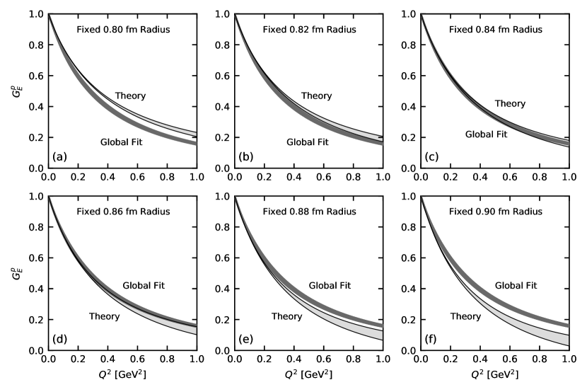
Figure 1: Light shaded bands between solid lines (labeled “Theory”): DI$\chi$EFT predictions of the proton charge FF $G_{E}^{p}(Q^{2})$ Alarcón and Weiss (2018b) for several values of the proton radius, $r_{E}^{p}=(0.80,0.82,0.84,0.86,0.88,0.90)$ fm (the values are indicated on the panels). The bands show the theoretical uncertainty resulting from the effective description of high-mass states in the spectral function (see text). Dark shaded bands (labeled “Global Fit”): $G_{E}^{p}(Q^{2})$ determined from global fits of the elastic FF data with constrained proton radius (see text) Ye et al. (2018). The bands show the experimental and fit uncertainties. Each panel’s global fit was restricted to reproduce the indicated proton radius.

II Method

II.1 Predictive theoretical framework

DI$\chi$EFT is a method for calculating the nucleon FFs combining chiral effective field theory ($\chi$EFT) — a systematic description of strong interactions at distances $\mathcal{O}(M_{\pi}^{-1})$; and dispersion analysis — the use of complex analyticity for connecting the behavior of hadronic amplitudes in different kinematic regions. The method is described in detail in Refs. Alarcón and Weiss (2017, 2018a, 2018b); the essential elements used in the present calculation are summarized for reference in Appendix A. The FFs are represented as dispersive integrals over $t\equiv-Q^{2}$. The spectral functions on the two-pion cut at $t>4M_{\pi}^{2}$ are calculated using (i) the elastic unitarity relation; (ii) $\pi N$ amplitudes computed in $\chi$EFT at leading order, next-to-leading order, and partial next-to-next-to-leading order accuracy; (iii) the timelike pion FF measured in $e^{+}e^{-}$ annihilation experiments. The approach includes $\pi\pi$ rescattering effects and the $\rho$ resonance and allows one to calculate the two-pion spectral functions up to $t\approx 1$ GeV². Higher-mass $t$-channel states are described by effective poles, whose strength is fixed by the dispersive integrals for the nucleon charges, magnetic moments, and radii (sum rules) Alarcón and Weiss (2018b). The nucleon radii thus enter as explicit parameters in the DI$\chi$EFT predictions of the spectral functions. Evaluating the finite-$Q^{2}$ dispersive integrals with these spectral functions, we obtain an analytic parametrization of the spacelike FFs in which the nucleon radii appear as explicit parameters [see Appendix A, specifically Eqs. (16) and (17)]; all other dynamical input is determined independently by the $\pi N$ scattering data and the pion timelike FF data. We emphasize that in this approach the correlation between the radius and the finite-$Q^{2}$ behavior appears through the global analytic properties of the FF (dispersive representation, sum rules), not through a power series expansion at $Q^{2}=0$; the correlation therefore extends beyond the range of convergence of the power series expansion (the connection with the power series expansion is discussed further in Sec. IV.2).

In the application here we take the proton charge radius as a free parameter, to be varied over a range covering the presently discussed values. The neutron charge radius, which enters indirectly through the separate sum rules for the isovector and isoscalar FFs, is fixed at its Particle Data Group (PDG) value Tanabashi et al. (2018); its influence on the proton FF is negligible in the $Q^{2}$ region considered here (see Appendix A, specifically Fig. 5). In this way DI$\chi$EFT provides us with a family of theoretical predictions of $G_{E}^{p}(Q^{2})$, with each function respecting analyticity in $Q^{2}$ and corresponding to definite value of the proton charge radius. Figure 1 shows the predictions for a set of radii $r_{E}^{p}=(0.80,0.82,0.84,0.86,0.88,0.90)$ fm.

The dominant uncertainties in the DI$\chi$EFT predictions of $G_{E}^{p}(Q^{2})$ (for a given $r_{E}^{p}$) arise from the the effective description of high-mass states in the isovector spectral function. We have estimated them conservatively, by varying the position of the effective pole over a range $M_{1}^{2}=$ (0.5–2)$\times M_{1}^{2}(\textrm{nom})$, where $M_{1}^{2}(\textrm{nom})$ is the nominal value determined in Ref. Alarcón and Weiss (2018b) [see Appendix A, specifically Eq. (6)]. The results are shown by the bands in Fig. 1. One sees that the uncertainties of the FF predictions are small at low $Q^{2}$ (where the dispersive integral is dominated by the two-pion cut and constrained by the given value of the radius), but increase at larger $Q^{2}$ (where the dispersive integral becomes sensitive to high-mass states in the spectral function).

II.2 Descriptive global fit

In order to confront the DI$\chi$EFT predictions with the experimental proton FF we use the results of a descriptive global fit Ye et al. (2018). It employs a bounded polynomial $z$-expansion Hill and Paz (2010) and determines $G_{E}^{p}$ and $G_{M}^{p}$ directly from the cross section and polarization data. Sum rules are imposed to ensure the correct normalization at $Q^{2}=0$ and the asymptotic scaling behavior at large $Q^{2}$ Lee et al. (2015). The treatment of uncertainties includes the covariance matrix of the fit itself, the systematic errors arising from the tension between data sets, and the uncertainty from two-photon exchange corrections at high $Q^{2}$. In the original work of Ref. Ye et al. (2018) the proton radii in the fit were fixed at their presumed empirical values ($r_{E}^{p}$ = 0.879 fm from CODATA, $r_{M}^{p}$ = 0.851 fm from PDG); the radius constraints were then removed when evaluating the fit uncertainty. In the present study we have used the same fitting method to generate a family of fits with different values of the proton charge radius, covering the range 0.8–0.9 fm (see Fig. 1). The magnetic radius is kept fixed at its PDG value; the uncertainty resulting from this simplification is negligible and covered by the quoted overall fit uncertainty. In these fits we only include the uncertainties from the covariance matrix. One observes that in the global fits there is little correlation between the proton charge radius and the value of the FFs at finite $Q^{2}$ (the present data cover the range $\gtrsim$ 0.01 GeV²), as expected for this descriptive approach.

II.3 Method for radius extraction

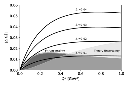
Figure 2: Light shaded band (labeled “Theory Uncertainty”): Theoretical uncertainty of the DI$\chi$EFT predictions of $G_{E}^{p}(Q^{2})$ for fixed $r_{E}^{p}$ (here $r_{E}^{p}=$ 0.84 fm; the uncertainty does not depend on the specific value of $r_{E}^{p}$; cf. Fig. 1) Alarcón and Weiss (2018b). Dark shaded band and dashed area above (labeled “Fit Uncertainty”): Experimental uncertainty of the global FF fit Ye et al. (2018) (68% confidence level, cf. Fig. 1). The dark shaded band shows the uncertainty of the fits with a fixed proton radius, as shown in the individual panels of Fig. 1. The dashed area above shows in addition the variation of the global fit under changes of the radius. Solid lines: Variation of the DI$\chi$EFT predictions of $G_{E}^{p}(Q^{2})$ under changes of $r_{E}^{p}$ by $\Delta r=\pm$0.01 fm, $\pm$0.02 fm, etc. (the variation is computed at $r_{E}^{p}=$ 0.84 fm). The variation quantifies the sensitivity of the theoretical FF predictions to the proton radius parameter (cf. Fig. 1).

Figure 1 now allows us to compare the DI$\chi$EFT predictions with the global fits to the FF data for several assumed values of the proton radius. We observe: (a) Whereas the global fits show little correlation between the radius and the finite-$Q^{2}$ FF, the DI$\chi$EFT predictions show a strong correlation, as a consequence of the analytic properties. (b) There is a clearly preferred value of the radius at $\sim$0.84 fm, for which there is best agreement of the DI$\chi$EFT predictions with the global fit to the FF data. (c) At the radius of best agreement, the DI$\chi$EFT predictions provide a description of the data with the same accuracy as the global fit up to $Q^{2}\sim 1$ GeV² (actually up to even larger values $Q^{2}\sim 2$ GeV², which are not included in Fig. 1).

The observations suggest a simple method for extracting the proton radius from the FF data: Compare the DI$\chi$EFT predictions with the global fit in the region where both descriptions are valid, and determine the radius by best agreement. The method combines the advantages of the descriptive fit (reliable uncertainty estimates in the region where there are data) and the predictive theory (correlation of the radius and the finite-$Q^{2}$ behavior through analyticity).

The method can be optimized by choosing the “best” $Q^{2}$ region for the comparison. Figure 2 shows the theoretical uncertainty of the DI$\chi$EFT FF prediction for a fixed proton radius, and the experimental uncertainties of the FF obtained from the global fit. It also shows the variation of the DI$\chi$EFT FF predictions under a certain change of the proton radius (here, $\Delta r=\pm$0.01 fm, $\pm$0.02 fm, etc.), which quantifies the sensitivity of the FF to the proton radius as a function of $Q^{2}$. One observes: (a) At “low” $Q^{2}$ ($\sim$0.1 GeV²) the theoretical uncertainty of the DI$\chi$EFT FF is much smaller than the experimental uncertainty of the global fit, which is mainly due to normalization errors (inconsistencies between data sets). The variation of the FF under the change $\Delta r=\pm 0.01$ is larger than the theoretical uncertainty but smaller than the fit uncertainty. (b) At “high” $Q^{2}$ ($\sim$1 GeV²) the theoretical uncertainty is larger than the fit uncertainty. The variation of the FF under $\Delta r=\pm 0.01$ is smaller than the theoretical uncertainty and comparable to the fit uncertainty. Based on Fig. 2 we choose the upper limit of the $Q^{2}$-region for radius extraction as $Q^{2}_{\rm max}\sim 0.5$ GeV²; with this upper limit the theoretical error remains smaller than, or at most comparable to, the fit error. The lower limit we choose as $Q^{2}_{\rm min}\sim$ 0.01 GeV²; this represents the lowest value for which FF data are presently available, and the results are not sensitive to this choice. (The performance of our method with smaller values of $Q^{2}_{\rm max}$ and the relation to low-$Q^{2}$ fits using a power series expansion are discussed in Sec. IV.2.)

To quantify the agreement of the theoretical model with the global fit and extract the radius, we use a figure of merit in the form of a reduced $\chi^{2}$,

$$\chi^{2}(r_{E}^{p}) \equiv N^{-1}\sum_{\textrm{bins $i$}}\frac{(\textrm{thy}_{i}-\textrm{fit}_{i})^{2}}{(\Delta\textrm{thy}_{i})^{2}+(\Delta\textrm{fit}_{i})^{2}}$$ (1)

$$\left\{\textrm{thy}_{i}\equiv G_{E}^{p}(Q^{2}_{i})\;[\textrm{DI$\chi$EFT, given $r_{E}^{p}$}],\right.$$

$$\left.\;\;\textrm{fit}_{i}\equiv G_{E}^{p}(Q^{2}_{i})\;[\textrm{global fit, given $r_{E}^{p}$}]\right\}.$$

The sum runs over $N$ bins in $Q^{2}$ covering the range $(Q^{2}_{\rm min},Q^{2}_{\rm max})$; we use $N=$ 50; the results are not sensitive to the binning. $\textrm{thy}_{i}$ denotes the DI$\chi$EFT prediction of $G_{E}^{p}(Q_{i}^{2})$ in the $i$’th $Q^{2}$ bin for the given $r_{E}^{p}$; $\textrm{fit}_{i}$ denotes the global fit result for $G_{E}^{p}(Q_{i}^{2})$ in the same bin. The theoretical and fit uncertainties, $\Delta\textrm{thy}_{i}$ and $\Delta\textrm{fit}_{i}$, are added in quadrature. Figure 3 shows the reduced $\chi^{2}$ as a function of $r_{E}^{p}$. One observes: (a) The dependence is approximately quadratic, indicating a natural best agreement without tension. (b) If the uncertainty of $r_{E}^{p}$ is defined by the criterion $\Delta\chi^{2}\leq 1$, the results obtained with $Q^{2}_{\rm max}=$ 0.4, 0.5, and 0.6 GeV² are consistent within uncertainties, affirming our choice of the optimal $Q^{2}_{\rm max}$.

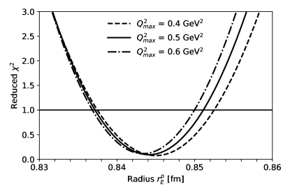
Figure 3: Reduced $\chi^{2}$, Eq. (1), as a function of the proton radius $r_{E}^{p}$. Shown are the results corresponding to three choices of the upper limit $Q^{2}_{\rm max}$.

III Results

Using the above method and $Q^{2}$-range, we have extracted the proton charge radius and its uncertainty, obtaining a value $r_{E}^{p}$ = 0.844(7) fm. The uncertainty estimate is based on the combined theoretical and global fit uncertainties entering in our figure of merit Eq. (1) and corresponds to a confidence interval with $\Delta\chi^{2}\leq 1$. The extracted radius is consistent with the high-precision muonic hydrogen results and clearly disfavors the CODATA result. Our result therefore suggests that the finite-$Q^{2}$ electron scattering data agree well with the muonic hydrogen results, and that the disagreement is rather between the electronic and muonic hydrogen results. We note that some recent measurements with electronic hydrogen have yielded a value consistent with the muonic result Beyer et al. (2017), while others agree with the current CODATA value Fleurbaey et al. (2018).

IV Discussion

IV.1 Possible improvements

The proton radius extraction reported here could be improved in several aspects: (a) by reducing the theoretical uncertainty of the DI$\chi$EFT FF predictions through an improved description of the high-mass spectral functions ($t>$ 1 GeV²), which would be possible with a more flexible parametrization and further theoretical constraints; (b) by reducing the experimental uncertainties of the FF data, especially in the region $Q^{2}\lesssim$ 0.2 GeV², which would allow us to limit the theory-experiment comparison to a smaller $Q^{2}$-interval ($Q^{2}_{\rm max}\sim$ 0.2 GeV²), where the theoretical uncertainties are smaller.

In our analyticity-based framework the main impact on the proton radius comes from FF data at moderate $Q^{2}$ ($\sim$ 0.1–0.5 GeV²) rather than at the lowest available $Q^{2}$. The forthcoming FF data at very low $Q^{2}$ from the Jefferson Lab PRad experiment Gasparian (2014) (down to a few $\times 10^{-4}$ GeV²) can complement the results of our study by reducing the normalization errors of the data (cf. the discussion below) and enabling an independent radius extraction using traditional extrapolation methods. They can also validate our theoretical framework, e.g. by extracting higher FF derivatives, which enable sensitive tests of the DI$\chi$EFT spectral functions Alarcón and Weiss (2018a).

IV.2 Relation to low-$Q^{2}$ FF fits

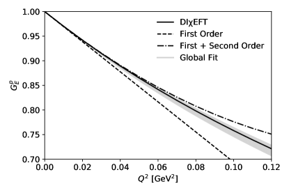
Figure 4: Low-$Q^{2}$ behavior of the DI$\chi$EFT parametrization of $G_{E}^{p}(Q^{2})$ and its power expansion. Solid line: DI$\chi$EFT parametrization ($r_{E}^{p}=0.844$ fm). Dashed line: First-order term in $Q^{2}$. Dashed-dotted line: Sum of first- and second-order terms. Shaded band: Uncertainty of the global fit with the given fixed proton radius.

In Ref. Horbatsch et al. (2017) the proton radius was extracted from fits to the low-$Q^{2}$ FF data ($Q^{2}_{\rm max}\lesssim 0.02$ GeV²) with a truncated power series in $Q^{2}$, in which the coefficient of the first-order term in $Q^{2}$ (the proton radius) was determined by the data, and the coefficients of the higher-order terms $Q^{4},Q^{6},$ etc. (the higher moments) were calculated in standard $\chi$EFT and supplied as a theoretical input. It is worth explaining how our dispersive method relates to that approach when the fit is restricted to the low-$Q^{2}$ region. Figure 4 shows the DI$\chi$EFT FF parametrization (with the radius determined by our above best fit), as well as its first-order and second-order expansion in $Q^{2}$; the coefficients are given by the derivatives of the FF, evaluated using the dispersive integral with the DI$\chi$EFT spectral functions. One sees that the full DI$\chi$EFT FF is well approximated by the second-order expansion, with the second-order term giving a correction of 1% (5%) at $Q^{2}=$ 0.03 GeV² (0.06 GeV²). The second derivative of the DI$\chi$EFT FF changes only by a few percent when the radius is varied within the range $r^{p}_{E}$ = (0.80, 0.90) fm, so that the coefficient of the second-order term may be regarded as a fixed theoretical input. Our method therefore effectively reduces to that of Ref. Horbatsch et al. (2017) in the region where the second-order approximation is valid ($Q^{2}_{\rm max}<0.05$ GeV²). The advantage of our method is that it is not limited by the power series expansion and allows us to include FF data at significantly higher $Q^{2}$ into the fit, making the radius extraction more robust. This can be seen in the trend shown in Fig. 3: increasing the value of $Q^{2}_{\rm max}$ decreases the uncertainty in the radius, as the fit is constrained by more data, while at the same time the theoretical uncertainties are still under control. For reference we note that, if we restricted our fit to $Q^{2}_{\rm max}=0.1$ GeV², we would obtain a radius $r^{p}_{E}$ = 0.849(10) fm, which agrees well with the result of Ref. Horbatsch et al. (2017) in the central value and the uncertainty.

We also point out that the second derivative (or moment) of the DI$\chi$EFT FF is significantly larger than the standard $\chi$EFT results used in Ref. Horbatsch et al. (2017), because the $\pi\pi$ rescattering effects included in the DI$\chi$EFT calculation increase the spectral function on the two-pion cut in the near-threshold region; see the discussion in Ref. Alarcón and Weiss (2018a). This shows that in the approach of Ref. Horbatsch et al. (2017) the theoretical uncertainty would deteriorate quickly if it were applied at $Q^{2}$ values where the second-order (and higher-order) terms become sizable. We note that the $\pi\pi$ rescattering effects are noticeable even in the higher FF derivatives ($n\geq 3$); nevertheless, for these quantities the DI$\chi$EFT results agree with the standard $\chi$EFT predictions within uncertainties; see Ref. Alarcón and Weiss (2018a) for details. Explicit expressions for the FF derivatives in standard $\chi$EFT can be found in Ref. Peset and Pineda (2014).

Some comments are in order regarding the experimental uncertainties in FF fits at low $Q^{2}$ ($\sim 0.01$ GeV²). The dominant uncertainty in this case results from the normalization errors of the FF data. In the fits the normalization of different data sets is adjusted, using the given fit function or theoretical model, and requiring that $G_{E}^{p}(0)=1$. Excellent fits can be achieved after this rescaling of the data sets, and one may be tempted to conclude that the radius could be extracted with great precision from them. However, such reasoning would be circular: The rescaling of the data sets depends on the fit function, and at low $Q^{2}$ the behavior of that function is governed by the radius, so that the procedure essentially forces the rescaled data to reproduce the assumed radius, resulting in a loss of sensitivity to the radius. This effect can be seen in the global fit uncertainties shown in Fig. 2. The dark shaded band shows the uncertainty of the global fit for a certain fixed value of the radius, i.e., constraining the first-order term in the fit function. This uncertainty vanishes rapidly in the limit $Q^{2}\rightarrow 0$, reflecting the trivial fact that the constrained fit with an assumed radius reproduces that value of the radius. The dashed area above the dark shaded band shows the variation in the global fit result under a change of the radius by $\Delta r=\pm(0.01,0.02,0.03,0.04)$ fm. The combined area represents the actual experimental uncertainty in the radius extraction in low-$Q^{2}$ fits. It is much larger than the fixed-radius uncertainty at low $Q^{2}$ and vanishes much more slowly in the $Q^{2}\rightarrow 0$ limit. Altogether, this points to a principal limitation of radius extraction from fits to low-$Q^{2}$ FF data. Our DI$\chi$EFT method overcomes this limitation by recruiting higher-$Q^{2}$ data for the radius extraction (up to $Q^{2}_{\rm max}\sim 0.5$ GeV²), whose impact is only minimally affected by normalization errors.

IV.3 Relation to empirical dispersive fits

The proton radius was extracted previously from dispersive FF fits in which the two-pion spectral functions were constructed by analytic continuation of empirical $\pi N$ amplitudes Belushkin et al. (2007); Lorenz et al. (2012). In these approaches the two-pion spectral functions are completely determined before they are placed in the dispersive integrals and used to evaluate FFs and radii. Our method is different in that the two-pion spectral functions are computed in DI$\chi$EFT and contain an unknown low-energy constant (related to the nucleon radii, cf. Appendix A), which can vary and adjust the strength of the spectral functions in the $\rho$ meson peak and above Alarcón and Weiss (2018b). This increases the flexibility of the FF description and enables a more robust radius extraction. We point out that the DI$\chi$EFT spectral functions at partial N2LO accuracy, evaluated with a realistic range of proton radii, agree very well with those of the Roy-Steiner analysis of Ref. Hoferichter et al. (2016), but differ significantly from those of Refs. Belushkin et al. (2007); Lorenz et al. (2012) in the $\rho$ meson mass region; see Ref. Alarcón and Weiss (2018b) for a detailed comparison. Even so, the empirical dispersive fits have consistently obtained proton radii $\sim$ 0.84 fm Belushkin et al. (2007); Lorenz et al. (2012), in agreement with our result.

Appendix A Form factor parametrization

In this appendix we summarize the DI$\chi$EFT calculation of the nucleon FFs and describe the parametrization used in the radius extraction in the present work. Further information about the method and other applications can be found in Refs. Alarcón and Weiss (2017, 2018a, 2018b).

The nucleon electric FFs are separated into isovector and isoscalar components,

$$G_{E}^{p,n}=\pm G_{E}^{V}+G_{E}^{S},\hskip 20.00003ptG_{E}^{V,S}\equiv{\textstyle\frac{1}{2}}(G_{E}^{p}\mp G_{E}^{n}),$$ (2)

and represented as dispersive integrals over $t\equiv-Q^{2}$,

$$G^{V,S}_{E}(t)\;=\;\frac{1}{\pi}\int_{t_{\rm thr}}^{\infty}dt^{\prime}\;\frac{\text{Im}\,G^{V,S}_{E}(t^{\prime})}{t^{\prime}-t-i0}.$$ (3)

The integrands involve the imaginary parts of the FFs on the cuts at $t^{\prime}>t_{\rm thr}>0$, which are known as the spectral functions. In the isovector component $t_{\rm thr}=4M_{\pi}^{2}$, and the spectral function is organized as

$$\text{Im}\,G^{V}_{E}(t^{\prime})\;=\;\text{Im}\,G^{V}_{E}(t^{\prime})[\pi\pi]\;+\;\text{Im}\,G^{V}_{E}(t^{\prime})[\textrm{high-mass}].$$ (4)

The first term accounts for the contribution of the two-pion cut from $t_{\rm thr}$ up to $t_{\rm max}\sim$ 1 GeV² and is calculated theoretically using the elastic unitarity relation in the $\pi\pi$ channel, the $\pi N$ amplitudes computed in $\chi$EFT, and the empirical timelike pion FF; the explicit expressions are given in Refs. Alarcón and Weiss (2018a, b). The couplings entering in the $\chi$EFT amplitudes at LO and NLO accuracy are determined by pion-nucleon scattering data. At partial N2LO accuracy the $\chi$EFT result involves one unknown low-energy constant, $\lambda$, which represents a free parameter; schematically

$$\text{Im}\,G^{V}_{E}[\pi\pi]\;=\;\textrm{[LO]}+\textrm{[NLO]}+\lambda\,\textrm{[N2LO]}.$$ (5)

The second term in Eq. (4) accounts for the high-mass states in the spectral function above $t_{\rm max}$ and is parametrized by an effective pole,

$$\text{Im}\,G^{V}_{E}(t^{\prime})[\textrm{high-mass}]\;=\;\pi a^{(1)}_{E}\,\delta(t^{\prime}-M_{1}^{2}),$$ (6)

where the pole position $M_{1}^{2}=2.1\,\textrm{GeV}^{2}$ is inferred from the $e^{+}e^{-}$ annihilation data and the pole strength represents a free parameter; the justification for this approximation and its accuracy are discussed in Ref. Alarcón and Weiss (2018b). The values of the parameters $\lambda$ and $a_{E}^{(1)}$ in Eqs. (5) and (6) are fixed by the sum rules for the nucleon isovector electric charge and radius,

$$\frac{1}{\pi}\int_{t_{\rm thr}}^{\infty}dt^{\prime}\,\frac{\text{Im}\,G_{E}^{V}(t^{\prime})}{t^{\prime}} = Q_{E}^{V}={\textstyle\frac{1}{2}},$$ (7)

$$\frac{6}{\pi}\int_{t_{\rm thr}}^{\infty}dt^{\prime}\,\frac{\text{Im}\,G_{E}^{V}(t^{\prime})}{t^{\prime 2}} = (r_{E}^{V})^{2}\equiv{\textstyle\frac{1}{2}}[(r_{E}^{p})^{2}-(r_{E}^{n})^{2}].\hskip 20.00003pt$$ (8)

Since the value of the isovector charge is known, this leaves the isovector radius as the only free parameter of the isovector spectral function Eq. (4). Note that the relation between the original parameters and the charge and radius implied by Eqs. (7) and (8) is linear,

$$\{\lambda,a_{E}^{(1)}\}\;\stackrel{{\scriptstyle\textrm{linear}}}{{\longleftrightarrow}}\;\{Q_{E}^{V},(r_{E}^{V})^{2}\}.$$ (9)

Expressing the parameters in terms of the radius, substituting the spectral function in Eq. (3), and performing the dispersive integral, we obtain a parametrization of the spacelike isovector FF ($t<0$) in the form

$$G_{E}^{V}(t)\;=\;A_{E}^{V}(t)\,+\,(r_{E}^{V})^{2}\,B_{E}^{V}(t).$$ (10)

The functions $A_{E}^{V}(t)$ and $B_{E}^{V}(t)$ represent, respectively, the dispersive integrals over the parts of the spectral function that are independent of $(r_{E}^{V})^{2}$, and proportional to $(r_{E}^{V})^{2}$. The functions have the same analytic structure as the full FF and embody the full complex $t$ dependence in the spacelike region, as dictated by the dispersive representation. Note that the linear decomposition in Eq. (10) results from the linear relation of $(r_{E}^{V})^{2}$ to the original theoretical parameters; it does not imply an expansion in $t$ or other approximation to the complex $t$-dependence of the FF.

In the isoscalar component of Eq. (3) $t_{\rm thr}=9M_{\pi}^{2}$, and the spectral function is parametrized as the sum of two effective poles,

$$\text{Im}\,G^{S}_{E}(t^{\prime})\,=\,\sum_{r=\omega,\phi}\pi a^{r}_{E}\delta(t^{\prime}-M_{r}^{2}).$$ (11)

The first pole is at the $\omega$ resonance mass and accounts for the $3\pi$ strength; the second pole is at the $\phi$ mass and effectively accounts for the $\phi$ resonance and other hadronic contributions at higher masses. The parameters $a_{E}^{\omega}$ and $a_{E}^{\phi}$ are fixed by the sum rules for the nucleon’s isoscalar electric charge and radius,

$$\frac{1}{\pi}\int_{t_{\rm thr}}^{\infty}dt^{\prime}\,\frac{\text{Im}\,G_{E}^{S}(t^{\prime})}{t^{\prime}} = Q_{E}^{S}={\textstyle\frac{1}{2}},$$ (12)

$$\frac{6}{\pi}\int_{t_{\rm thr}}^{\infty}dt^{\prime}\,\frac{\text{Im}\,G_{E}^{S}(t^{\prime})}{t^{\prime 2}} = (r_{E}^{S})^{2}\equiv{\textstyle\frac{1}{2}}[(r_{E}^{p})^{2}+(r_{E}^{n})^{2}],\hskip 30.00005pt$$ (13)

which imply a linear relation similar to Eq. (9). Altogether we obtain a representation of the spacelike isoscalar FF analogous to the isovector case, Eq. (10),

$$G_{E}^{S}(t)\;=\;A_{E}^{S}(t)\,+\,(r_{E}^{S})^{2}\,B_{E}^{S}(t).$$ (14)

Combining the isovector and isoscalar parametrizations, Eqs. (10) and Eqs. (14), we obtain a parametrization of the proton an neutron FFs in terms of the isovector and isoscalar radii,

$$G_{E}^{p,n}(t)\; = \;\pm A_{E}^{V}(t)\,+\,A_{E}^{S}(t)$$ (15)

$$\pm(r_{E}^{V})^{2}\,B_{E}^{V}(t)\,+\,(r_{E}^{S})^{2}\,B_{E}^{S}(t).$$

It may also be expressed directly in terms of the individual nucleon radii,

$$G_{E}^{p}(t)\, = \,A_{E}^{p}(t)\,+\,(r_{E}^{p})^{2}\,B_{E}(t)\,+\,(r_{E}^{n})^{2}\,\bar{B}_{E}(t),\hskip 10.00002pt\hskip 10.00002pt$$ (16)

$$G_{E}^{n}(t)\, = \,A_{E}^{n}(t)\,+\,(r_{E}^{n})^{2}\,B_{E}(t)\,+\,(r_{E}^{p})^{2}\,\bar{B}_{E}(t),\hskip 10.00002pt$$ (17)

where the functions are

$$A_{E}^{p,n} \equiv \pm A_{E}^{V}+A_{E}^{S},$$ (18)

$$B_{E} \equiv {\textstyle\frac{1}{2}}(B_{E}^{V}+B_{E}^{S}),$$ (19)

$$\bar{B}_{E} \equiv {\textstyle\frac{1}{2}}(-B_{E}^{V}+B_{E}^{S}).$$ (20)

The functions $A^{p,n}(t)$ describe the radius-independent part of the nucleon FFs (in the context of the dispersive parametrization defined above); the functions $B_{E}(t)$ and $\bar{B}_{E}(t)$ describe, respectively, the parts proportional to the charge radii of the “same” and the “other” nucleon, under the constraints of isospin symmetry. Several properties of the functions follow immediately from their definitions:

$$\left.\begin{array}[]{rclrcl}A_{E}^{p,n}(0)&=&Q_{E}^{p,n},&dA_{E}^{p,n}/dt(0)&=&0,\\[4.30554pt] B_{E}(0)&=&0,&6\;dB_{E}/dt(0)&=&1,\\[4.30554pt] \bar{B}_{E}(0)&=&0,&d\bar{B}_{E}/dt(0)&=&0,\end{array}\hskip 10.00002pt\right\}$$ (21)

where $Q_{E}^{p,n}=\{1,0\}$ is the nucleon electric charge. In particular, these conditions ensure that the nucleon FFs described by Eqs. (16) and (17) have the correct values at zero momentum transfer, $G_{E}^{p,n}(0)=Q_{E}^{p,n}$, and that the first derivatives of the nucleon FFs are controlled exclusively by the radii of the “same” nucleon,

$$6\,dG_{E}^{p,n}/dt(0) = 6\;dB_{E}/dt(0)\,(r_{E}^{p,n})^{2}\;=\;6\,(r_{E}^{p,n})^{2}.\hskip 30.00005pt$$ (22)

Figure 5: Proton FF parametrization Eq. (16) as function of $Q^{2}=-t$. Dashed line: $A_{E}^{p}(t)$. Dashed-dotted line: $A_{E}^{p}(t)+(r_{E}^{p})^{2}\,B_{E}(t)$. Solid line: $A_{E}^{p}(t)+(r_{E}^{p})^{2}\,B_{E}(t)+(r_{E}^{n})^{2}\,\bar{B}_{E}(t)$ (full result).

Figure 5 shows the contributions of the individual terms in the proton FF parametrization Eq. (16) as functions of $Q^{2}=-t$. One observes: (a) The radius-independent term $A_{E}^{p}$ starts with value 1 and derivative 0 at $Q^{2}=0$, cf. Eq. (21); its value remains close to 1 for all $Q^{2}<1$ GeV². (b) The proton-radius-dependent term $(r_{E}^{p})^{2}\,B_{E}$ starts with value 0 at $Q^{2}=0$ and accounts for the derivative of $G_{E}^{p}$ at $Q^{2}=0$; it causes most of the $Q^{2}$-dependence of the FF (i.e., the deviation of $G_{E}^{p}$ from 1) at $Q^{2}<1$ GeV². (c) The neutron-radius-dependent term $(r_{E}^{n})^{2}\,\bar{B}_{E}$ starts with value 0 and derivative 0 at $Q^{2}=0$; its contribution to $G_{E}$ remains $<0.01$ for $Q^{2}<1$ GeV². Altogether, the sum $A_{E}^{p}+(r_{E}^{p})^{2}\,B_{E}$ practically accounts for the entire value of the FF and its $Q^{2}$-dependence all at $Q^{2}<1$ GeV²; the $(r_{E}^{n})^{2}\,\bar{B}_{E}$ term represents a percent-level correction. This makes the parametrization Eq. (16) particularly useful for extracting the proton radius from the FF data. The parametrization of the neutron FF Eq. (17) follows the same pattern, with the role of the radii reversed.

The numerical evaluation of the FFs with the radius-dependent dispersive FF parametrizations, Eqs. (16) and (16), is extremely simple. The functions $A_{E}^{p,n}(t)$, $B_{E}(t)$ and $\bar{B}_{E}(t)$ can be pre-computed and tabulated as functions of $Q^{2}=-t$. The FFs are then generated by multiplying these functions with the radii and combining the terms. This method was used to produce the plots of Fig. 1 and perform the radius extraction summarized in Fig. 3. The parametrization can be used also in other studies of low-$Q^{2}$ proton and neutron FFs. Tables of the functions are are available upon request.