Geometric quench in the fractional quantum Hall effect: exact solution in quantum Hall matrix models and comparison with bimetric theory

Abstract

We investigate the recently introduced geometric quench protocol for fractional quantum Hall (FQH) states within the framework of exactly solvable quantum Hall matrix models. In the geometric quench protocol a FQH state is subjected to a sudden change in the ambient geometry, which introduces anisotropy into the system. We formulate this quench in the matrix models and then we solve exactly for the post-quench dynamics of the system and the quantum fidelity (Loschmidt echo) of the post-quench state. Next, we explain how to define a spin-2 collective variable $\hat{g}_{ab}(t)$ in the matrix models, and we show that for a weak quench (small anisotropy) the dynamics of $\hat{g}_{ab}(t)$ agrees with the dynamics of the intrinsic metric governed by the recently discussed bimetric theory of FQH states. We also find a modification of the bimetric theory such that the predictions of the modified bimetric theory agree with those of the matrix model for arbitrarily strong quenches. Finally, we introduce a class of higher-spin collective variables for the matrix model, which are related to generators of the $W_{\infty}$ algebra, and we show that the geometric quench induces nontrivial dynamics for these variables.

I Introduction

Topological phenomena in gapped fractional quantum Hall (FQH) states, such as anyonic excitations, robust edge modes, and ground state degeneracy on closed manifolds, are well-described by Chern-Simons topological quantum field theories Wen (2004). These theories apply in the limit in which the bulk energy gap is sent to infinity and so, by their very nature, they are incapable of describing the dynamics of gapped excitations in FQH states. Nevertheless, FQH states support a bulk gapped collective excitation known as the magneto-roton, or Girvin-MacDonald-Platzman (GMP) mode Girvin et al. (1986). For small wavevectors $\mathbf{k}$ the GMP mode is characterized by a definite angular momentum equal to $2\hbar$, i.e., the GMP mode is a “spin-2” mode near $\mathbf{k}=0$. Recently, a new effective “bimetric” field theory was developed Gromov et al. (2017); Gromov and Son (2017) to describe the gapped dynamics of this spin-2 mode. The fundamental degree of freedom in this theory is a dynamical unimodular metric $\hat{g}_{ab}(\mathbf{x},t)$, and the gapped fluctuations of this metric, which have spin-2, correspond to the dynamics of the GMP mode near $\mathbf{k}=0$. The development of the bimetric theory relied on the extensive body of work on geometry Abanov and Gromov (2014); Cho et al. (2014); Ferrari and Klevtsov (2014); Bradlyn and Read (2015a, b); Can et al. (2015); Gromov et al. (2015); Gromov and Abanov (2014); Karabali and Nair (2016); Haldane (2009, 2011); Park and Haldane (2014); You et al. (2014); Qiu et al. (2012); Gromov and Abanov (2015); Gromov et al. (2016); Can et al. (2014); Douglas and Klevtsov (2010); Klevtsov and Wiegmann (2015); Schine et al. (2016, 2018); Maciejko et al. (2013) and Hall viscosity Avron et al. (1995); Lévay (1995); Avron (1998); Tokatly and Vignale (2007); Read (2009); Tokatly and Vignale (2009); Haldane (2009, 2011); Read and Rezayi (2011); Hughes et al. (2011); Hoyos and Son (2012); Bradlyn et al. (2012); Park and Haldane (2014) in quantum Hall states from the past two decades.

Given the existence of interesting gapped excitations in FQH states, it is natural to try to engineer a situation in which the gapped dynamics of FQH states could be observed, either in numerical simulations or in experiments. With this goal in mind, a quantum quench protocol for FQH states, dubbed a “geometric quench”, was introduced in Ref. Liu et al., 2018. This geometric quench is designed for the express purpose of exciting the (neutral) gapped excitations in FQH systems, and can be summarized briefly as follows. First, we prepare the system in an isotropic FQH ground state $|\psi_{0}\rangle$ of an isotropic Hamiltonian $H_{0}$. Next, we suddenly change the Hamiltonian to incorporate some anisotropy, $H_{0}\to H^{\prime}$. Finally, we evolve the initial state forward in time using the new anisotropic Hamiltonian, $|\psi(t)\rangle=e^{-i\frac{H^{\prime}t}{\hbar}}|\psi_{0}\rangle$.

The authors of Ref. Liu et al., 2018 investigated this geometric quench in two ways. First, they studied the quench analytically using the aforementioned bimetric theory. Second, they studied the quench numerically using the recently introduced anisotropic Haldane pseudopotentials Yang et al. (2017). For quadropolar anisotropy parametrized by a constant unimodular metric $g_{ab}$, this quench was shown to excite the gapped spin-2 mode near $\mathbf{k}=0$ (i.e., the small $\mathbf{k}$ limit of the GMP mode). In addition, the dynamics of this mode in the case of small anisotropy was shown to be well-described by bimetric theory. Ref. Liu et al., 2018 also considered quenches with more complicated anisotropy, and these quenches were shown to excite exotic higher-spin modes, which have a larger excitation gap than the spin-2 mode. The existence of such higher-spin excitations in the FQH effect has been anticipated since early work on infinite-dimensional $W_{\infty}$ symmetry in FQH states Cappelli et al. (1993); Karabali (1994a, b); Flohr and Varnhagen (1994); Cappelli et al. (1994).

Our goal in this paper is to study the geometric quench protocol in more detail. To do so we consider this quench in the context of exactly solvable matrix models of FQH states. The exact solubility of these matrix models allows us to make significant analytical progress in studying the geometric quench. We focus most of our discussion on the matrix model for Laughlin states, known as the Chern-Simons matrix model (CSMM). The CSMM was introduced by Polychronakos Polychronakos (2001a), who proposed it as a concrete regularization of Susskind’s noncommutative Chern-Simons theory of the Laughlin states Susskind (2001), and the CSMM and noncommutative Chern-Simons theory were subsequently studied by many authors Polychronakos (2001b); Morariu and Polychronakos (2001); Hellerman and Van Raamsdonk (2001); Karabali and Sakita (2001, 2002); Hansson and Karlhede (2001); Fradkin et al. (2002); Hansson et al. (2003); Cappelli and Riccardi (2005); Tong and Turner (2015). We will also explain how our results for the Laughlin states extend to a matrix model for the Blok-Wen series Blok and Wen (1992) of non-Abelian FQH states. This non-Abelian matrix model was introduced and studied in detail in Refs. Dorey et al., 2016a, b (this model also appeared in Ref. Morariu and Polychronakos, 2001, but was given a different physical interpretation in that reference). In Refs. Lapa and Hughes, 2018; Lapa et al., 2018, it was shown that the matrix models accurately capture the geometric properties of the FQH states they describe. In particular, the correct value of the guiding center Hall viscosity of these FQH states can be recovered from the matrix model descriptions (see Refs. Haldane, 2009, 2011; Park and Haldane, 2014 for the concept of Landau orbit vs. guiding center contributions to the Hall viscosity). The fact that the CSMM and its non-Abelian generalizations accurately describe the geometric response of FQH states suggest that these models are ideal testing grounds for the geometric quench of Ref. Liu et al., 2018.

In this paper we formulate the geometric quench protocol in the CSMM for the case of quadropolar anisotropy parametrized by a constant unimodular metric $g_{ab}$. We then solve exactly for the post-quench state $|\psi(t)\rangle$ and compute the quantum fidelity $|\langle\psi_{0}|\psi(t)\rangle|^{2}$ (also known as the Loschmidt echo). We also define and compute the exact dynamics of a spin-2 collective variable that naturally emerges in the CSMM. We denote this collective variable by $\hat{g}_{ab}(t)$ because, as we show in the paper, this quantity is the analogue in the CSMM of the dynamical metric in bimetric theory. We show that $\hat{g}_{ab}(t)$ undergoes nonlinear oscillations after the quench, with a period set by the gap $E_{2}$ for spin-2 excitations in the CSMM. In the case of small anisotropy, we show that the dynamics of $\hat{g}_{ab}(t)$ in the CSMM coincides with the post-quench dynamics predicted by bimetric theory in Ref. Liu et al., 2018. We also generalize these results to the non-Abelian matrix model of Refs. Dorey et al., 2016a, b. These results imply that the quantum Hall matrix models can describe the numerical data of Ref. Liu et al., 2018 for small anisotropy just as well as bimetric theory.

We then explore the connection between the matrix models and bimetric theory in more detail, and we show that there exists a modified potential energy term for bimetric theory such that the predictions of the matrix models for the geometric quench exactly match the predictions of bimetric theory with the alternative potential energy term. Finally, in the last part of the paper we define a set of higher-spin collective variables for the CSMM and discuss their relation to previous work on higher-spin operators and $W_{\infty}$ symmetry in the CSMM. We then show that the geometric quench considered in this paper induces nontrivial dynamics for these higher-spin variables.

The CSMM is closely related to the Calogero model of interacting particles in one dimension (see Ref. Polychronakos, 2001a for the connection). Consequently, there is a relation between the geometric quench in the CSMM and the quench of the harmonic trap frequency in the Calogero model that was considered in Ref. Rajabpour and Sotiriadis, 2014. The main difference between the geometric quench for the CSMM and the work of Ref. Rajabpour and Sotiriadis, 2014 is that, in the language of the Calogero model, the geometric quench of the CSMM corresponds to a simultaneous quench of both the harmonic trap frequency and the mass of the Calogero particles (note that in the Calogero Hamiltonian the mass parameter appears as a coefficient in the kinetic energy term and the interaction term). Thus, the dynamics induced by the geometric quench in the CSMM is qualitatively distinct from that studied in Ref. Rajabpour and Sotiriadis, 2014. Another similar quench protocol was discussed in Franchini et al. (2015), where the harmonic trap frequency was quenched simultaneously with the interaction strength.

This paper is organized as follows. In Sec. II we review the CSMM and introduce various important variables and notation. In Sec. III we formulate and solve the geometric quench in the CSMM, and extend those results to the non-Abelian matrix model. In Sec. IV we give a detailed comparison of the predictions of the CSMM and bimetric theory, and we also discuss the new potential energy term for bimetric theory that we mentioned in the previous paragraph. In Sec. V we introduce a set of higher-spin collective variables for the CSMM, and we calculate their post-quench dynamics. Sec. VI presents our conclusions. Finally, several important formulas are contained in Appendices A, B, and C.

II Review of the Chern-Simons matrix model (CSMM)

II.1 Physical meaning of the model and summary of notation

In this section we give a lightning review of the CSMM and its quantization. We also highlight some specific properties of the quantum ground state of the CSMM which we use later in the paper in the solution of the geometric quench. For more details on this model and its physical interpretation we refer the reader to the original work Polychronakos (2001a), and to Lapa and Hughes (2018); Lapa et al. (2018) for a recent discussion in the context of geometric response of quantum Hall states (our notation is essentially the same as Ref. Lapa et al., 2018).

The degrees of freedom in the CSMM consist of two $N\times N$ Hermitian matrices $X^{a}(t)$, $a=1,2$, a complex length $N$ vector $\varphi(t)$, and an additional $N\times N$ Hermitian matrix $A_{0}(t)$ which is a $U(N)$ gauge field. All of these degrees of freedom are functions of time $t$. We denote the matrix elements of the matrix degrees of freedom by ${(X^{a})^{j}}_{k}$, $j,k=1,\dots,N$ (and likewise for $A_{0}$), and the components of $\varphi$ by $\varphi^{j}$, $j=1,\dots,N$.

The physical meaning of the CSMM can be briefly summarized as follows. The starting point for this interpretation is Susskind’s noncommutative Chern-Simons theory description of the Laughlin states Susskind (2001). In that description a quantum Hall state is modeled as a fluid on the “noncommutative plane”, a deformation of the two-dimensional plane $\mathbb{R}^{2}$ in which the coordinates $x^{a}$ are promoted to operators $\hat{x}^{a}$ which obey a nontrivial commutation relation $[\hat{x}^{1},\hat{x}^{2}]=i\theta$, where $\theta$ is a constant with units of length squared. In Susskind’s model $\theta$ is quantized as

$$\theta=\ell_{B}^{2}m\ ,m\in\mathbb{Z}\ ,$$ (1)

where $\ell_{B}^{2}=\frac{\hbar}{eB}$ is the square of the magnetic length. The integer $m$, which we take to be positive, is related to the filling fraction of the Laughlin state by

$$\nu=\frac{1}{m}\ .$$ (2)

This can be seen from the fact that the density of the fluid in Susskind’s model is related to $\theta$ by

$$\overline{\rho}=\frac{1}{2\pi\theta}=\frac{1}{2\pi\ell_{B}^{2}m}\ ,$$ (3)

which is exactly the mean density of the $\nu=\frac{1}{m}$ Laughlin state. The physical interpretation of the parameter $\theta$ is that $2\pi\theta$ is the area occupied by a single electron in Susskind’s model. In Susskind (2001) it was argued that due to the finite value of the parameter $\theta$, the noncommutative Chern-Simons theory accurately captures the “granularity” of a fluid composed of discrete particles (which are electrons in this case).

The CSMM can be viewed as a regularization of Susskind’s noncommutative Chern-Simons theory. While the latter theory describes a constant density fluid occupying the entire noncommutative plane, the CSMM describes a finite droplet of fluid on the noncommutative plane consisting of $N$ electrons. Indeed, the eigenvalues of the matrices $X^{a}$ in the CSMM can be interpreted as the coordinates of electrons on the plane. Since the matrices $X^{a}$ do not commute with each other in the CSMM (i.e., they are not simultaneously diagonalizable), the electrons described by the CSMM still live on the noncommutative plane. For further details on the physical interpretation of the CSMM we refer the reader to Susskind (2001); Polychronakos (2001a); Lapa and Hughes (2018).

Before moving on, we summarize our notations. When the matrix model is quantized, the matrix elements of $X^{a}$ and $A_{0}$, as well as the components of $\varphi$, become operators on a quantum Hilbert space. In what follows we reserve the symbol “$\dagger$” to denote Hermitian conjugation of quantum operators. For classical matrix and vector degrees of freedom we use a superscript “$T$” to denote a transpose and an overline to denote complex conjugation. We also use the notation $[\cdot,\cdot]_{M}$ to denote the commutator of classical matrix degrees of freedom (“$M$” stands for matrix). The notation $[\cdot,\cdot]$ without any subscript will be used for the commutator of quantum operators. Finally, $\text{Tr}\{\cdot\}$ always denotes the trace of classical matrices.

II.2 CSMM and its quantization

The action for the CSMM has the form

$$S_{0} =-\frac{eB}{2}\int_{0}^{T}dt\ \text{Tr}\Big{\{}\epsilon_{ab}X^{a}\mathcal{D}_{0}X^{b}+2\theta A_{0}$$

$$+ \ \omega\delta_{ab}X^{a}X^{b}\Big{\}}+i\int_{0}^{T}dt\ \overline{\varphi}^{T}\mathcal{D}_{0}\varphi\ ,$$ (4)

where the covariant derivatives $\mathcal{D}_{0}X^{b}$ and $\mathcal{D}_{0}\varphi$ are defined as

$$\mathcal{D}_{0}X^{b} = \dot{X}^{b}-i[A_{0},X^{b}]_{M}$$ (5a)

$$\mathcal{D}_{0}\varphi = \dot{\varphi}-iA_{0}\varphi\ ,$$ (5b)

and the dot denotes an ordinary time derivative. Here we work on a time interval $t\in[0,T)$, and we impose periodic boundary conditions in time on all degrees of freedom. This turns the time-direction into a circle of circumference $T$, which we denote by $S^{1}_{T}$. Just as in Susskind’s model, the parameter $\theta$ is quantized as $\theta=\ell_{B}^{2}m\ ,\ m\in\mathbb{Z}$ and we again choose $m>0$. In this case the CSMM describes the Laughlin state with $\nu=\frac{1}{m}$.

The quantization rule for $\theta$ comes from requiring the exponential $e^{i\frac{S_{0}}{\hbar}}$ of the action to be invariant under large $U(N)$ gauge transformations. The action $S_{0}$ is nearly invariant under the $U(N)$ gauge transformation

$$X^{a} \to VX^{a}\overline{V}^{T}$$ (6a)

$$A_{0} \to VA_{0}\overline{V}^{T}+iV\dot{\overline{V}}^{T}$$ (6b)

$$\varphi \to V\varphi\ ,$$ (6c)

where $V(t)$ is a time-dependent $U(N)$ matrix. However, the term in the Lagrangian proportional to $\text{Tr}\{A_{0}\}$ spoils this invariance. This is because of the existence of large gauge transformations in which the map $V:S^{1}_{T}\to U(N)$ corresponds to a nontrivial element of the group $\pi_{1}(U(N))=\mathbb{Z}$. Requiring invariance of $e^{i\frac{S_{0}}{\hbar}}$ under these large gauge transformations then gives the quantization rule for $\theta$.

In the CSMM the gauge field $A_{0}$ enforces the constraint ($\mathbb{I}$ is the $N\times N$ identity matrix)

$$G:=ieB[X^{1},X^{2}]_{M}+eB\theta\mathbb{I}-\varphi\overline{\varphi}^{T}=0\ ,$$ (7)

and in the $A_{0}=0$ gauge the Hamiltonian takes the form

$$H_{0}=\frac{eB\omega}{2}\text{Tr}\{\delta_{ab}X^{a}X^{b}\}\ .$$ (8)

This Hamiltonian represents a harmonic trap for the noncommutative fluid described by the CSMM, and the strength of this trap is set by the frequency $\omega$.

To quantize the model it is convenient to define a set of real scalar variables which serve to completely specify the matrices $X^{a}$. In the quantized model these variables then become Hermitian operators. To define these real scalar variables we introduce a basis $T^{A}$, $A=0,\dots,N^{2}-1,$ of generators of the Lie algebra of $U(N)$ in the fundamental representation. Thus, $T^{A}$ are $N\times N$ Hermitian matrices, and we assume they are normalized so that $\text{Tr}\{T^{A}T^{B}\}=\delta^{AB}$. A concrete choice for the generators $T^{A}$ is to choose $T^{0}=\frac{\mathbb{I}}{\sqrt{N}}$, and so $T^{0}$ is the generator of the $U(1)$ part of $U(N)$. For $A\neq 0$ we choose $T^{A}=\sqrt{2}t^{A}$, where $t^{A}$ are a basis of conventionally normalized generators of $SU(N)$ which satisfy $\text{Tr}\{t^{A}t^{B}\}=\frac{\delta^{AB}}{2}$ and $[t^{A},t^{B}]_{M}=i\sum_{C}f^{ABC}t^{C}$, where $f^{ABC}$ are the structure constants of $SU(N)$ (we do not need to know the exact form of $f^{ABC}$ in this paper). Using this basis we then parametrize $X^{a}(t)$ as

$$X^{a}(t)=\sum_{A=0}^{N^{2}-1}x^{a}_{A}(t)T^{A}\ ,$$ (9)

where we have introduced $2N^{2}$ real scalar variables $x^{a}_{A}(t)$. In the quantized CSMM these scalar variables obey the commutation relations

$$[x^{a}_{A},x^{b}_{B}]=i\ell_{B}^{2}\epsilon^{ab}\delta_{AB}\ ,$$ (10)

where are very similar to the commutation relations of guiding center coordinates in the quantum Hall problem.

Using these new scalar variables we define the oscillator variables

$$z_{A}=\frac{1}{\ell_{B}\sqrt{2}}(x^{1}_{A}+ix^{2}_{A})\ ,$$ (11)

and $z^{\dagger}_{A}=\frac{1}{\ell_{B}\sqrt{2}}(x^{1}_{A}-ix^{2}_{A})$. We also define

$$b^{j}=\frac{1}{\sqrt{\hbar}}\varphi^{j}\ ,$$ (12)

and $b^{\dagger}_{j}=\frac{1}{\sqrt{\hbar}}\overline{\varphi}_{j}$ (here $\overline{\varphi}_{j}$ are the components of the row vector $\overline{\varphi}^{T}$). In the quantized CSMM these variables all obey the harmonic oscillator commutation relations

$$\left[z_{A},z^{\dagger}_{B}\right] = \delta_{AB}$$ (13a)

$$\left[b^{j},b^{\dagger}_{k}\right] = \delta^{j}_{k}\ .$$ (13b)

For later use we also define the matrix-valued operators $Z^{\pm}$ whose matrix elements are given by

$${(Z^{-})^{j}}_{k} = \sum_{A=0}^{N^{2}-1}z_{A}{(T^{A})^{j}}_{k}$$ (14a)

$${(Z^{+})^{j}}_{k} = \sum_{A=0}^{N^{2}-1}z^{\dagger}_{A}{(T^{A})^{j}}_{k}\ .$$ (14b)

The commutation relations of $z_{A}$ and $z^{\dagger}_{B}$ then imply that

$$\left[{(Z^{-})^{j}}_{k},{(Z^{+})^{\ell}}_{m}\right]=\delta^{j}_{m}\delta^{\ell}_{k}\ .$$ (15)

If we quantize the CSMM in the $A_{0}=0$ gauge, then gauge invariance requires that all states in the physical Hilbert space of the model be annihilated by the matrix elements ${G^{j}}_{k}$ of the constraint $G$ from Eq (7). A useful way to think about these constraints is to define a new set of constraints by taking the trace with the $U(N)$ generators $T^{A}$, i.e., we define new constraints $G^{A}:=\text{Tr}\{GT^{A}\}$. Let $|\text{phys}\rangle$ denote a state in the physical Hilbert space of the model. Then the constraints $G^{A}|\text{phys}\rangle=0$ for $A\neq 0$ imply that all physical states transform as singlets under the $SU(N)$ part of $U(N)$. The remaining constraint $G^{0}|\text{phys}\rangle=0$ can be shown to reduce to

$$b^{\dagger}_{j}b^{j}|\text{phys}\rangle=N(m-1)|\text{phys}\rangle\ .$$ (16)

This constraint implies that all physical states carry a total charge of $N(m-1)$ under the $U(1)$ part of $U(N)$. Note also that $G^{A}|\text{phys}\rangle=0$ for all $A$ implies that ${G^{j}}_{k}|\text{phys}\rangle=0$ for all $j,k$, since the ${G^{j}}_{k}$ are linear combinations of the $G^{A}$.

Let $|0\rangle$ be the Fock vacuum state which is annihilated by the $z_{A}$ and $b^{j}$ operators. Then a complete basis of physical states for the CSMM consists of the states Hellerman and Van Raamsdonk (2001)

$$|\{c_{1},\dots,c_{N}\}\rangle =$$

$$\text{Tr}\{Z^{+}\}^{c_{1}} \text{Tr}\{(Z^{+})^{2}\}^{c_{2}}\cdots\text{Tr}\{(Z^{+})^{N}\}^{c_{N}}|\psi_{0}\rangle$$ (17)

where $c_{j}\in\mathbb{N}$ for $j=1,\dots,N$, and

$$|\psi_{0}\rangle=\left(\epsilon^{j_{1}\cdots j_{N}}b^{\dagger}_{j_{1}}[b^{\dagger}Z^{+}]_{j_{2}}\cdots[b^{\dagger}(Z^{+})^{N-1}]_{j_{N}}\right)^{(m-1)}|0\rangle\ .$$ (18)

In the $A_{0}=0$ gauge the CSMM Hamiltonian can be rewritten in the form

$$H_{0}=\hbar\omega\frac{N^{2}}{2}+\hbar\omega\sum_{A=0}^{N^{2}-1}z^{\dagger}_{A}z_{A}\ ,$$ (19)

which is equal to a constant plus a term proportional to the total number operator for the $z_{A}$ oscillators. From this it is clear that the lowest energy physical state is $|\psi_{0}\rangle$, with energy

$$E_{0}=\hbar\omega\left[\frac{1}{2}mN^{2}+\left(\frac{1-m}{2}\right)N\right]\ .$$ (20)

The other states $|\{c_{1},\dots,c_{N}\}\rangle$ can be seen to have an energy of

$$E(\{c_{1},\dots,c_{N}\})=E_{0}+\hbar\omega\sum_{j=1}^{N}c_{j}j\ .$$ (21)

For later use we also define a dimensionless ground state energy $\epsilon_{0}$ by

$$\epsilon_{0}:=\frac{E_{0}}{\hbar\omega}\ .$$ (22)

We also mention here that the angular momentum operator $L_{z}$ for the CSMM takes the form

$$L_{z}=-\frac{eB}{2}\text{Tr}\{\delta_{ab}X^{a}X^{b}\}\ .$$ (23)

In particular, it is clear that $L_{z}=-\frac{1}{\omega}H_{0}$. It follows that the state $|\{c_{1},\dots,c_{N}\}\rangle$ has angular momentum

$$L_{z}(\{c_{1},\dots,c_{N}\})=-\hbar\epsilon_{0}-\hbar\sum_{j=1}^{N}c_{j}j\ .$$ (24)

II.3 $sl(2,\mathbb{R})$ generators

The matrices $X^{a}$ can be interpreted as Lagrangian coordinates for a fluid on the noncommutative plane Susskind (2001). To investigate the response of this fluid to changes in the geometry, we need to identify the operators which generate area-preserving diffeomorphisms (APDs) of the fluid coordinates. The group $\text{SDiff}(\mathbb{R}^{2})$ of APDs of the plane is an infinite-dimensional group whose elements are (smooth, invertible) functions $\eta:\mathbb{R}^{2}\to\mathbb{R}^{2}$ which preserve the volume form $\text{vol}=dx^{1}\wedge dx^{2}$ on $\mathbb{R}^{2}$, i.e., $\eta^{*}\text{vol}=\text{vol}$, where $\eta^{*}$ denotes the pullback along the map $\eta$. This group has a finite-dimensional subgroup isomorphic to $SL(2,\mathbb{R})$ which consists of the functions $\eta$ of the form

$$\eta^{a}(x)={A^{a}}_{b}x^{b}\ ,$$ (25)

where ${A^{a}}_{b}$ are the components of a $2\times 2$ real matrix $A$ with determinant $1$, i.e., an element of $SL(2,\mathbb{R})$. Note here that ${A^{a}}_{b}$ has no $x$ dependence. One can think of this subgroup of $\text{SDiff}(\mathbb{R}^{2})$ as being equal to the subset of APDs which are uniform in space.

It was shown in Lapa and Hughes (2018) that the operators which generate these $SL(2,\mathbb{R})$ transformations for the matrix coordinates $X^{a}$ are

$$\mathsf{\Lambda}^{ab}=\frac{1}{4\ell_{B}^{2}}\sum_{A=0}^{N^{2}-1}\{x^{a}_{A},x^{b}_{A}\}\ ,$$ (26)

where $\{\cdot,\cdot\}$ denotes an anti-commutator, and one can check that these operators obey,

$$[\mathsf{\Lambda}^{ab},\mathsf{\Lambda}^{cd}]=\frac{i}{2}\left(\epsilon^{bc}\mathsf{\Lambda}^{ad}+\epsilon^{bd}\mathsf{\Lambda}^{ac}+\epsilon^{ac}\mathsf{\Lambda}^{bd}+\epsilon^{ad}\mathsf{\Lambda}^{bc}\right)\ ,$$ (27)

which are the commutation relations for the Lie algebra $sl(2,\mathbb{R})$.

Finite $SL(2,\mathbb{R})$ transformations of the noncommutative coordinates are implemented by conjugation by a unitary operator $U(\alpha)=e^{i\alpha_{ab}\mathsf{\Lambda}^{ab}}$, where $\alpha_{ab}$ is a constant symmetric matrix which parametrizes the deformation. To first order in $\alpha_{ab}$ we have (for all $j,k$)

$$U(\alpha){(X^{a})^{j}}_{k}U(\alpha)^{\dagger}={(X^{a})^{j}}_{k}+\epsilon^{ab}\alpha_{bc}{(X^{c})^{j}}_{k}+\cdots$$ (28)

Since the operators $U(\alpha)$ act identically on all matrix elements ${(X^{a})^{j}}_{k}$ of the noncommutative coordinates $X^{a}$, the operators $\mathsf{\Lambda}^{ab}$ can indeed be interpreted as generating $SL(2,\mathbb{R})$ transformations of the noncommutative coordinates $X^{a}$.

It is convenient to introduce another basis for the generators of $sl(2,\mathbb{R})$, which have the form

$$K_{0} = \frac{1}{2}\Big{(}\mathsf{\Lambda}^{11}+\mathsf{\Lambda}^{22}\Big{)}$$ (29)

$$K_{-} = \frac{1}{2}\Big{(}\mathsf{\Lambda}^{11}-\mathsf{\Lambda}^{22}\Big{)}+i\mathsf{\Lambda}^{12}$$ (30)

$$K_{+} = (K_{-})^{\dagger}.$$ (31)

This basis of generators obeys the algebra

$$[K_{0},K_{\pm}] = \pm K_{\pm}$$ (32a)

$$\left[K_{-},K_{+}\right] = 2K_{0}\ ,$$ (32b)

and in this form the $sl(2,\mathbb{R})$ algebra is also known as $su(1,1)$.

One fact which will be useful later in the paper is that $K_{-}$ annihilates the ground state $|\psi_{0}\rangle$ of the original CSMM,

$$K_{-}|\psi_{0}\rangle=0\ ,$$ (33)

and this can be shown using a proof by contradiction. Suppose instead that $K_{-}|\psi_{0}\rangle\neq 0$. Then, since $K_{-}$ is invariant under the $U(N)$ action in the CSMM (this can be seen by writing it as a trace, $K_{-}=\frac{1}{2}\text{Tr}\{(Z^{-})^{2}\}$), the state $K_{-}|\psi_{0}\rangle$ is also a valid state in the physical Hilbert space of the matrix model. In addition, this state has energy $E_{0}-2\hbar\omega$ for the Hamiltonian $H_{0}$. Therefore $K_{-}|\psi_{0}\rangle$, if different from zero, would be a new physical state of the CSMM with lower energy than the ground state $|\psi_{0}\rangle$. This is a contradiction since it is already known that $|\psi_{0}\rangle$ has the lowest eigenvalue of $H_{0}$ among all of the physical states of the model. Therefore it must be that $K_{-}|\psi_{0}\rangle=0$. Note that this proof also generalizes to a proof that $|\psi_{0}\rangle$ is annihilated by all the $U(N)$-invariant operators $\text{Tr}\{(Z^{-})^{p}\}$ for $p=1,\dots,N$, with $K_{-}$ corresponding to the case of $p=2$.

II.4 Introducing anisotropy into the CSMM

We now explain how to introduce anisotropy into the CSMM. One way to do this, following Lapa and Hughes (2018), is to deform the harmonic trap by replacing the Kronecker delta $\delta_{ab}$ with a constant unimodular metric $g_{ab}$ (i.e., a constant metric with determinant equal to one). The nontrivial metric $g_{ab}$ represents some externally imposed anisotropy in the problem. The action for this modified CSMM takes the form

$$S_{g} =-\frac{eB}{2}\int_{0}^{T}dt\ \text{Tr}\Big{\{}\epsilon_{ab}X^{a}\mathcal{D}_{0}X^{b}+2\theta A_{0}$$

$$+ \ \omega g_{ab}X^{a}X^{b}\Big{\}}+i\int_{0}^{T}dt\ \overline{\varphi}^{T}\mathcal{D}_{0}\varphi\ ,$$ (34)

in which the only change to the action is the replacement $\delta_{ab}\to g_{ab}$ in the harmonic potential term. In the $A_{0}=0$ gauge the Hamiltonian for this modified matrix model is

$$H_{g}=\frac{eB\omega}{2}\text{Tr}\{g_{ab}X^{a}X^{b}\}\ .$$ (35)

This model was solved in Lapa and Hughes (2018) and we mention here some of the important properties of this model. First, the entire energy spectrum of this model is identical to that of the CSMM with $g_{ab}=\delta_{ab}$ (this statement is only true because $g_{ab}$ has determinant one). In particular, the quantum ground state $|\psi_{g}\rangle$ of this model has the same energy $E_{0}$ as the ground state $|\psi_{0}\rangle$ of the original CSMM. In addition, the expectation value of the $sl(2,\mathbb{R})$ generators $\mathsf{\Lambda}^{ab}$ in the state $|\psi_{g}\rangle$ is given by

$$\langle\psi_{g}|\mathsf{\Lambda}^{ab}|\psi_{g}\rangle=\frac{\epsilon_{0}}{2}g^{ab}\ ,$$ (36)

where $g^{ab}$ is the inverse metric for $g_{ab}$. It was shown in Lapa and Hughes (2018) that, as a consequence of this relation, the Hall viscosity of this modified CSMM with $\theta=\ell_{B}^{2}m$ is equal to the guiding center Hall viscosity of the Laughlin $\nu=\frac{1}{m}$ state with guiding center metric $g_{ab}$ Haldane (2009, 2011).

This calculation also suggests a way to define an intrinsic metric $\hat{g}_{ab}$ associated with any state $|\psi\rangle$ in the matrix model. We define $\hat{g}_{ab}$ by first defining its inverse $\hat{g}^{ab}$ to be proportional to the expectation value $\langle\psi|\mathsf{\Lambda}^{ab}|\psi\rangle$. In the special case that $|\psi\rangle$ is chosen to be the ground state $|\psi_{g}\rangle$ of the CSMM with metric $g_{ab}$, Eq. (36) shows that the intrinsic metric $\hat{g}_{ab}$ associated with this state is locked to the externally imposed metric $g_{ab}$. Later in the paper we use the intuition provided by this example to define a time-dependent intrinsic metric $\hat{g}_{ab}(t)$ in a time-dependent state $|\psi(t)\rangle$ obtained after performing a geometric quench in the CSMM.

Finally we note that the Hamiltonian $H_{g}$ can be written in terms of the $sl(2,\mathbb{R})$ generators as

$$H_{g}=\hbar\omega g_{ab}\mathsf{\Lambda}^{ab}\ .$$ (37)

In this form the Hamiltonian of the CSMM resembles the Hamiltonian of the bimetric theory, as we discuss later.

III Geometric quench in the CSMM and its exact solution

In this section we formulate the geometric quench protocol in the CSMM, and we also define a time-dependent intrinsic metric in the post-quench state. We then present the exact solution for the post-quench state and the time-dependent intrinsic metric. We show that our results agree with the results obtained in Liu et al. (2018) using bimetric theory in the limit of small anisotropy (we give a more detailed comparison with the bimetric theory results later in Sec. IV). Finally, at the end of this section we show how our results for the CSMM can be extended to the case of the non-Abelian matrix model of Refs. Dorey et al., 2016a, b.

III.1 Geometric quench protocol in the CSMM

The geometric quench of a FQH state was introduced in Ref. Liu et al., 2018 and consists of a sudden change in the background geometry in a FQH system. This quench can be formulated in the CSMM as follows. We start with the system in the ground state $|\psi_{0}\rangle$ of the original CSMM. Then, at time $t=0$, we suddenly introduce anisotropy into the system by replacing $\delta_{ab}\to g_{ab}$ in the harmonic trap term of the CSMM (we still take $g_{ab}$ to be a constant unimodular metric). As result, the initial state $|\psi_{0}\rangle$ evolves in time under the influence of the Hamiltonian $H_{g}$ of the CSMM with nontrivial metric $g_{ab}$ from Eq. (34). Mathematically, the post-quench state at time $t$ is related to the initial state as

$$|\psi(t)\rangle=e^{-i\frac{H_{g}t}{\hbar}}|\psi_{0}\rangle\ .$$ (38)

One of our main results in this section is an explicit expression for the post-quench state $|\psi(t)\rangle$.

Given the post-quench state $|\psi(t)\rangle$, we can define a time-dependent intrinsic metric using Eq. (36) as a guide. We denote this metric by $\hat{g}_{ab}(t)$ and we define it by first defining its inverse $\hat{g}^{ab}(t)$ as

$$\hat{g}^{ab}(t):=\frac{2}{\epsilon_{0}}\langle\psi(t)|\mathsf{\Lambda}^{ab}|\psi(t)\rangle\ .$$ (39)

The normalization factor here can be understood by comparison with Eq. (36), and with this normalization $\hat{g}_{ab}(t)$ will also be a unimodular metric (this will be verified by an explicit computation). The “dynamical metric” $\hat{g}_{ab}(t)$ is a spin-$2$ collective variable, which (partially) characterizes the many-body dynamics of the CSMM.

For easy comparison with Ref. Liu et al., 2018, we choose the anisotropy metric $g_{ab}$ to be of the form

$$g=\begin{pmatrix}e^{A}&0\\ 0&e^{-A}\end{pmatrix}\ ,$$ (40)

where $A$ is a real parameter which determines the anisotropy ($g_{ab}$ are the components of the matrix $g$). This choice of metric stretches the system along one axis (the $x^{1}$-axis for $A>0$), while squashing the system along the other axis. The fact that $g_{ab}$ is diagonal means that there is no additional rotation off of the main coordinate axes. This choice of $g_{ab}$ makes our calculations in this section slightly easier, however, the case of a non-diagonal $g_{ab}$ can be dealt with using the same methods.

To make contact with Ref. Liu et al., 2018 we also parametrize the dynamical metric $\hat{g}_{ab}(t)$ using a a real parameter $Q(t)\geq 0$ and a real phase $\phi(t)$. In this parametrization the metric takes the form considered in Liu et al. (2018),

$$\hat{g}=\begin{pmatrix}\cosh(Q)+\cos(\phi)\sinh(Q)&\sin(\phi)\sinh(Q)\\ \sin(\phi)\sinh(Q)&\cosh(Q)-\cos(\phi)\sinh(Q)\end{pmatrix}\ .$$ (41)

One can check that this does indeed define a unimodular metric. We now proceed with the exact calculations of $|\psi(t)\rangle$ and $\hat{g}_{ab}(t)$.

III.2 Post-quench state and the quantum fidelity (Loschmidt echo)

To determine the post-quench state $|\psi(t)\rangle$ we first note that using expression (37), the Hamiltonian $H_{g}$ for our specific choice of $g_{ab}$ takes the form

$$H_{g}=\hbar\omega\big{(}\sinh(A)K_{+}+2\cosh(A)K_{0}+\sinh(A)K_{-}\big{)}\ .$$ (42)

Then, using the rearrangement identity (111) from Appendix A, we can rewrite the time evolution operator $e^{-i\frac{H_{g}t}{\hbar}}$ as

$$e^{-i\frac{H_{g}t}{\hbar}}=e^{-\beta(t)K_{+}}e^{\ln(\delta(t))K_{0}}e^{-\beta(t)K_{-}}\ ,$$ (43)

where $\beta(t),\delta(t)$ are functions of $t,\omega,A$, and are given explicitly in Eqs. (112) and (113) of Appendix A. If we now use the fact that $K_{-}|\psi_{0}\rangle=0$, then we find that

$$|\psi(t)\rangle=e^{-\beta(t)K_{+}}e^{\ln(\delta(t))K_{0}}|\psi_{0}\rangle\ .$$ (44)

In addition, from the definition of $K_{0}$ it is clear that $K_{0}|\psi_{0}\rangle=\frac{\epsilon_{0}}{2}|\psi_{0}\rangle$ (since $K_{0}=\frac{1}{2}\frac{H_{0}}{\hbar\omega}$), and so our final answer for the time-evolved state is

$$|\psi(t)\rangle=[\delta(t)]^{\frac{\epsilon_{0}}{2}}e^{-\beta(t)K_{+}}|\psi_{0}\rangle\ .$$ (45)

We see that the quench excites all even spin excitations, since acting with $K_{+}$ changes the angular momentum of a state by $-2\hbar$ (recall that the angular momentum operator $L_{z}$ for the CSMM has the form shown in Eq. (23)). Indeed, we can write $K_{+}=\frac{1}{2}\text{Tr}\{(Z^{+})^{2}\}$ in terms of the matrix-valued operator $Z^{+}$, and $\text{Tr}\{(Z^{+})^{2}\}$ is the operator which creates spin-2 excitations over the ground state $|\psi_{0}\rangle$ of the original CSMM (recall the form of the excited states $|\{c_{1},\dots,c_{N}\}\rangle$ for the original CSMM from Eq. (17)).

We close this subsection by computing the quantity $|\langle\psi_{0}|\psi(t)\rangle|^{2}$, which is also known as the quantum fidelity or Loschmidt echo. The result is

$$|\langle\psi_{0}|\psi(t)\rangle|^{2}= \left[\delta(t)\overline{\delta(t)}\right]^{\frac{\epsilon_{0}}{2}}$$

$$= \left[\cos^{2}(\omega t)+\cosh^{2}(A)\sin^{2}(\omega t)\right]^{-\epsilon_{0}}$$

$$= \left[1+\sinh^{2}(A)\sin^{2}(\omega t)\right]^{-\epsilon_{0}}\ ,$$ (46)

where we plugged in for $\delta(t)$ using the explicit expression from Appendix A. Since $\sin^{2}(\omega t)$ has a period of $T=\frac{\pi}{\omega}$, we find that the quantum fidelity oscillates at the period

$$T=\frac{\pi}{\omega}\equiv\frac{2\pi\hbar}{E_{2}}\ ,$$ (47)

where

$$E_{2}:=2\hbar\omega$$ (48)

is the gap for spin-2 excitations in the CSMM. The actual magnitude of the overlap depends on the filling fraction $\nu=\frac{1}{m}$ through the power of $\epsilon_{0}$. Note also that since $\sinh^{2}(A)\sin^{2}(\omega t)\geq 0$, the fidelity satisfies $|\langle\psi_{0}|\psi(t)\rangle|^{2}\leq 1$.

Recall that the parameter $\epsilon_{0}$ has the form $\epsilon_{0}=\frac{1}{2}mN^{2}+\frac{(1-m)}{2}N$, and so the quantum fidelity $|\langle\psi_{0}|\psi(t)\rangle|^{2}$ has a factor of $N^{2}$ appearing in the exponent. To eliminate this large factor it is convenient to compare the values of the quantum fidelity between integer and fractional cases. Let $\mathcal{F}_{\frac{1}{m}}(t)$ denote the fidelity $|\langle\psi_{0}|\psi(t)\rangle|^{2}$ for the CSMM with $\theta=\ell_{B}^{2}m$ corresponding to the $\nu=\frac{1}{m}$ Laughlin state. Then we consider the following ratio of $\mathcal{F}_{\frac{1}{m}}(t)$ with $\mathcal{F}_{1}(t)$ raised to the $m^{th}$ power,

$$\frac{\left[\mathcal{F}_{1}(t)\right]^{m}}{\mathcal{F}_{\frac{1}{m}}(t)} = \left[1+\sinh^{2}(A)\sin^{2}(\omega t)\right]^{-\left(\frac{m-1}{2}\right)N}$$ (49)

$$= \left[1+\sinh^{2}(A)\sin^{2}(\omega t)\right]^{-\varsigma N}\ ,$$

where

$$\varsigma=\frac{m-1}{2}$$ (50)

is the anisospin Gromov et al. (2017); Gromov and Son (2017) for the $\nu=\frac{1}{m}$ Laughlin state, also called (minus) the guiding center spin Haldane (2009, 2011). For small anisotropy $A\ll 1$ this is ratio is approximately equal to

$$\frac{\left[\mathcal{F}_{1}(t)\right]^{m}}{\mathcal{F}_{\frac{1}{m}}(t)}\approx 1-\varsigma NA^{2}\sin^{2}(\omega t)\ .$$ (51)

We see that by comparing the fidelity for $\nu=\frac{1}{m}$ with the fidelity for $\nu=1$, we are able to extract the universal data $\varsigma$ which characterizes the $\nu=\frac{1}{m}$ Laughlin state. This type of comparison with the $\nu=1$ state is very similar to the comparison which is used to extract the dipole moment per unit length at the edge of a FQH state Wiegmann (2012); Park and Haldane (2014) (the dipole moment also happens to be proportional to the same parameter $\varsigma$ as it is closely related to the guiding center part of the bulk Hall viscosity).

Finally, for comparison to numerics it is useful to rewrite Eq. (49) in terms of the filling fraction $\nu=\frac{1}{m}$ and the energy gap $E_{2}=2\hbar\omega$ for the spin-2 mode, which gives

$$\frac{\left[\mathcal{F}_{1}(t)\right]^{\nu^{-1}}}{\mathcal{F}_{\nu}(t)} =\left[1+\sinh^{2}(A)\sin^{2}\left(\frac{E_{2}t}{2\hbar}\right)\right]^{-\varsigma N}$$ (52a)

$$\approx 1-\varsigma NA^{2}\sin^{2}\left(\frac{E_{2}t}{2\hbar}\right)\ ,$$ (52b)

where in the second line we Taylor-expanded the result for small $A$. In this form, the expression for $\frac{\left[\mathcal{F}_{1}(t)\right]^{\nu^{-1}}}{\mathcal{F}_{\nu}(t)}$ suggests a way to extract the anisospin $\varsigma$ and the spin-2 gap $E_{2}$ for a general FQH state with filling fraction $\nu$ by fitting numerical data from the simulation of a geometric quench for that FQH state to Eq. (52b). Indeed, preliminary numerical results Liu and Papić suggest that the formula (52b) is a good fit to the quantum fidelity for the geometric quench considered in Liu et al. (2018). Note also that for comparison to numerics $E_{2}$ is expected to equal the energy gap of the GMP mode at $\mathbf{k}=0$.

III.3 Dynamics of the intrinsic metric

In this subsection we present the exact calculation of the dynamical metric $\hat{g}_{ab}(t)$. We then show that for small anisotropy $A$, the CSMM result agrees with the bimetric theory results of Ref. Liu et al., 2018. We give a more detailed comparison with bimetric theory in Sec. IV.

We start by using the form of $|\psi(t)\rangle$ derived in the last subsection to write the formula for the inverse metric $\hat{g}^{ab}(t)$ in the form

$$\hat{g}^{ab}(t)=\frac{2}{\epsilon_{0}}\left[\delta(t)\overline{\delta(t)}\right]^{\frac{\epsilon_{0}}{2}}\langle\psi_{0}|e^{-\overline{\beta(t)}K_{-}}\mathsf{\Lambda}^{ab}e^{-\beta(t)K_{+}}|\psi_{0}\rangle\ .$$ (53)

We know that the $sl(2,\mathbb{R})$ generators $\mathsf{\Lambda}^{ab}$ can be expressed in terms of the $su(1,1)$ generators $K_{0},K_{\pm}$, and so we choose to proceed with this calculation by first calculating the expectation values $\langle\psi_{0}|e^{-\overline{\beta(t)}K_{-}}K_{0}e^{-\beta(t)K_{+}}|\psi_{0}\rangle$ and $\langle\psi_{0}|e^{-\overline{\beta(t)}K_{-}}K_{\pm}e^{-\beta(t)K_{+}}|\psi_{0}\rangle$.

To calculate these expectation values we use a generating function technique. We define a function $f(a,b,c)$ of three variables $a,b,c$ by

$$f(a,b,c):=\langle\psi_{0}|e^{aK_{-}}e^{bK_{0}}e^{cK_{+}}|\psi_{0}\rangle\ .$$ (54)

Then the expectation values which we are interested in can be computed from $f(a,b,c)$ as

$$\langle\psi_{0}|e^{-\overline{\beta(t)}K_{-}}K_{-}e^{-\beta(t)K_{+}}|\psi_{0}\rangle =\frac{\partial f(a,b,c)}{\partial a}\Bigg{|}_{a=-\overline{\beta(t)},\ b=0,\ c=-\beta(t)}$$ (55)

$$\langle\psi_{0}|e^{-\overline{\beta(t)}K_{-}}K_{0}e^{-\beta(t)K_{+}}|\psi_{0}\rangle =\frac{\partial f(a,b,c)}{\partial b}\Bigg{|}_{a=-\overline{\beta(t)},\ b=0,\ c=-\beta(t)}$$ (56)

$$\langle\psi_{0}|e^{-\overline{\beta(t)}K_{-}}K_{+}e^{-\beta(t)K_{+}}|\psi_{0}\rangle =\frac{\partial f(a,b,c)}{\partial c}\Bigg{|}_{a=-\overline{\beta(t)},\ b=0,\ c=-\beta(t)}\ .$$ (57)

The function $f(a,b,c)$ itself can be calculated using the rearrangement identity Eq. (115) from Appendix A, combined with the fact that $K_{-}|\psi_{0}\rangle=0$. Using that information, we find that

$$f(a,b,c)=[b^{\prime}(a,b,c)]^{\frac{\epsilon_{0}}{2}}\ ,$$ (58)

where the new function $b^{\prime}(a,b,c)$ is written down explicitly in Eq. (117) of Appendix A.

The calculation now proceeds in a straightforward manner and we find that the metric $\hat{g}_{ab}(t)$ (which is the inverse of $\hat{g}^{ab}(t)$) can be written in matrix form as

$$\hat{g}(t)=\frac{1}{1-|\beta(t)|^{2}}\begin{pmatrix}(1+\beta(t))(1+\overline{\beta(t)})&-i(\beta(t)-\overline{\beta(t)})\\ -i(\beta(t)-\overline{\beta(t)})&(1-\beta(t))(1-\overline{\beta(t)})\end{pmatrix}\ .$$ (59)

where $\beta(t)$ is again the function defined in Eq. (112) of Appendix A. We also note here that in order to derive these expressions we needed to use the formula Eq. (114).

From Eq. (112) we can see that the parameter $\beta(t)$ oscillates with a period of $T=\frac{\pi}{\omega}=\frac{2\pi\hbar}{E_{2}}$ ($E_{2}=2\hbar\omega$ was defined in Eq. (48)), and its time average is

$$\langle\beta(t)\rangle=\frac{1}{T}\int_{0}^{T}dt\ \beta(t)=\tanh\left(\frac{A}{2}\right)\ .$$ (60)

It is interesting to note that if we replace $\beta(t)$ with $\langle\beta(t)\rangle$ in the metric $\hat{g}_{ab}(t)$, then the dynamical metric reduces to the metric $g_{ab}$ from Eq. (40) that we used for the quench Hamiltonian $H_{g}$.

We now study the CSMM solution for the dynamical metric in the case of small anisotropy $A\ll 1$, because in this case we can compare to the results of Liu et al. (2018) obtained using the linearized equations of motion of bimetric theory. To compare our dynamical metric $\hat{g}_{ab}(t)$ with the one obtained in Liu et al. (2018), we write the complex parameter $\beta(t)$ in terms of a real parameter $Q(t)$ and a real phase $\phi(t)$ as

$$\beta(t)=\tanh\left(\frac{Q(t)}{2}\right)e^{i\phi(t)}\ .$$ (61)

With this parametrization the dynamical metric $\hat{g}_{ab}(t)$ takes the form shown in Eq. (41) and used in Liu et al. (2018). Note that in this parametrization one should always choose $Q(t)\geq 0$ so that there is no redundancy in the description (all information about the phase of $\beta(t)$ should be packaged in the parameter $\phi(t)$). In this case we find that $Q(t)$ is related to $\beta(t)$ as

$$Q(t)=2\tanh^{-1}\left[\sqrt{|\beta(t)|^{2}}\right]\ ,\quad\phi(t)=\text{arg}[\beta(t)]\ .$$ (62)

For small anisotropy the parameter $Q(t)$ in the solution for the dynamical metric is expected to be small, and so in this case we can write

$$\beta(t)\approx\frac{Q(t)}{2}e^{i\phi(t)}\ .$$ (63)

On the other hand, for small $A$ the exact solution for $\beta(t)$ from the CSMM takes the form

$$\beta(t) \approx \frac{A}{1-i\cot(\omega t)}$$ (64)

$$= A\sin(\omega t)e^{-i\omega t+i\frac{\pi}{2}}\ .$$

By comparing these two expressions for $\beta(t)$ we obtain the solution for $Q(t)$ and $\phi(t)$ for the case of small $A$ (we assume $A>0$),

$$Q(t) = 2A\left|\sin\left(\frac{E_{2}}{2\hbar}t\right)\right|$$ (65)

$$\phi(t) = \pi-\frac{E_{2}}{2\hbar}t-\frac{\pi}{2}\text{sgn}\left[\sin\left(\frac{E_{2}}{2\hbar}t\right)\right]\ ,$$ (66)

where $E_{2}=2\hbar\omega$ is the gap for the spin-2 mode in the CSMM. These equations exactly match the predictions of bimetric theory, as these solutions are identical to Eq. 5 of Liu et al. (2018), which is a solution to the linearized equations of motion Eqs. 20 and 21 of Liu et al. (2018) for the geometric quench in bimetric theory.

For the case of arbitrary anisotropy $A$ the CSMM predicts that the dynamical metric $\hat{g}_{ab}(t)$ undergoes nonlinear oscillations, in the sense that the amplitude of the function $\beta(t)$ is a nonlinear function of $A$. However, these oscillations still have a definite period $T=\frac{2\pi\hbar}{E_{2}}$ set by the energy gap $E_{2}$ of the spin-2 mode in the CSMM, so the period of the oscillations is independent of the amplitude.

For small anisotropy $A\ll 1$ the linearized solution and the full solution are nearly identical. However, the difference between these two solutions can be seen clearly in the case of a quench with large anisotropy (see Fig. 1 for details).

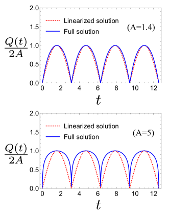
Figure 1: Plots of the linearized solution for $Q(t)$ (dotted red line) and the full nonlinear solution (blue line) for the case of medium anisotropy $A=1.4$ and large anisotropy $A=5$, both normalized by dividing by $2A$. The time axis is plotted in units with $\omega=1$. The maximum value of $Q(t)/(2A)$ is $1$ and occurs (for $\omega=1$) when $t=\pi/2+\pi n$ for any integer $n$. For smaller $A$ the linearized solution is close to the full solution, while for larger $A$ the full nonlinear solution has a much rounder profile than the linearized solution.

III.4 Extension to the non-Abelian Blok-Wen states

We close this section with a discussion of how our results extend to the matrix model for the non-Abelian Blok-Wen series of FQH states Dorey et al. (2016a, b) (see also Ref. Lapa et al., 2018 for the calculation of the Hall viscosity in this matrix model).

The main difference between the CSMM and the non-Abelian matrix model (NAMM) is that instead of having just one complex vector $\varphi$, the NAMM has $p$ complex vectors $\varphi_{\alpha}$, $\alpha=1,\dots,p$, for some positive integer $p$. The action for the NAMM takes the form

$$S^{\text{{\tiny{(NA)}}}}_{0} =-\frac{eB}{2}\int_{0}^{T}dt\ \text{Tr}\Big{\{}\epsilon_{ab}X^{a}\mathcal{D}_{0}X^{b}+2\theta A_{0}$$

$$+ \ \omega\delta_{ab}X^{a}X^{b}\Big{\}}+i\sum_{\alpha=1}^{p}\int_{0}^{T}dt\ \overline{\varphi}^{T}_{\alpha}\mathcal{D}_{0}\varphi_{\alpha}\ ,$$ (67)

and one can see that this action has an additional $SU(p)$ global symmetry which rotates the different $\varphi_{\alpha}$ into each other. In this model it is also convenient to parametrize $\theta$ (which is still quantized to be an integer) as

$$\theta=\ell_{B}^{2}(k+p)\ ,$$ (68)

for some other integer $k$, and we assume that $k$ is chosen so that $k+p\geq 0$. The NAMM then describes the subset of the Blok-Wen states at filling

$$\nu=\frac{p}{k+p}\ ,$$ (69)

and the $\nu=1/(k+1)$ Laughlin state is recovered from this model upon setting $p=1$ (so for $p=1$, set $k+1=m$ to compare with our previous results on the CSMM). In addition, it is known Lapa et al. (2018) that the anisospin $\varsigma$ for these states is independent of $p$ and given by

$$\varsigma=\frac{k}{2}\ .$$ (70)

We now give a brief summary of the quantization of this model. First, the $b_{j}$ variables from earlier acquire an additional index $\alpha$, so that we now have $pN$ oscillator variables $b^{j}_{\alpha}$ and their Hermitian conjugates $b^{\dagger}_{\alpha,j}$, and these obey $[b^{j}_{\alpha},b^{\dagger}_{\beta,\ell}]=\delta^{j}_{\ell}\delta_{\alpha\beta}$. Next, the constraint enforced by $A_{0}$ is now modified to

$$G:=ieB[X^{1},X^{2}]_{M}+eB\theta\mathbb{I}-\sum_{\alpha=1}^{p}\varphi_{\alpha}\overline{\varphi}^{T}_{\alpha}=0\ .$$ (71)

The $SU(N)$ part of this constraint still requires physical states to be $SU(N)$ singlets, but the $U(1)$ part of the constraint now takes the form

$$\sum_{\alpha=1}^{p}b^{\dagger}_{\alpha,j}b^{j}_{\alpha}|\text{phys}\rangle=Nk|\text{phys}\rangle$$ (72)

for all physical states $|\text{phys}\rangle$. On the other hand, the Hamiltonian $H_{0}$ (in the $A_{0}=0$ gauge) and angular momentum operator $L_{z}$ for the NAMM are identical to those in the CSMM. Thus, anisotropy parametrized by $g_{ab}$ is introduced into the Hamiltonian in the same way as for the CSMM and the geometric quench protocol for the NAMM is exactly the same as for the CSMM.

Finally, we come to the construction of the quantum ground state of the NAMM. Here we consider only the case where $N$ is divisible by $p$, because in this case the ground state is unique (see Ref. Dorey et al., 2016a, b for more details and the general case). To construct the ground state we first construct, for any integer $r\geq 0$, the operator

$$\mathcal{B}^{\dagger}(r)_{j_{1}\cdots j_{p}}:=\epsilon^{\alpha_{1}\cdots\alpha_{p}}[b^{\dagger}_{\alpha_{1}}(Z^{\dagger})^{r}]_{j_{1}}\cdots[b^{\dagger}_{\alpha_{p}}(Z^{\dagger})^{r}]_{j_{p}}\ .$$ (73)

This operator is a singlet under the global $SU(p)$ symmetry of the model, but it is not invariant under the $SU(N)$ gauge symmetry. An operator which is invariant under both the $SU(p)$ global symmetry and the $SU(N)$ gauge symmetry can then be constructed from the $\mathcal{B}^{\dagger}(r)_{j_{1}\cdots j_{p}}$ operators as

$$\tilde{\mathcal{B}}:=\epsilon^{j_{1}\cdots j_{N}} \mathcal{B}^{\dagger}(0)_{j_{1}\cdots j_{p}}\mathcal{B}^{\dagger}(1)_{j_{p+1}\cdots j_{2p}}$$

$$\cdots\mathcal{B}^{\dagger}({N}/{p}-1)_{j_{N-p+1}\cdots j_{N}}\ .$$ (74)

Finally, the unique ground state of the NAMM can be constructed using $\tilde{\mathcal{B}}$ as

$$|\psi^{\text{{\tiny{(NA)}}}}_{0}\rangle=\tilde{\mathcal{B}}^{k}|0\rangle\ .$$ (75)

In particular, the power of $k$ here ensures that Eq. (72) is satisfied. The energy of the ground state is

$$E^{\text{{\tiny{(NA)}}}}_{0}=\hbar\omega\left[\left(\frac{k+p}{p}\right)\frac{N^{2}}{2}-\frac{k}{2}N\right]\ ,$$ (76)

and we again define the dimensionless quantity

$$\epsilon^{\text{{\tiny{(NA)}}}}_{0}:=\frac{E^{\text{{\tiny{(NA)}}}}_{0}}{\hbar\omega}\ .$$ (77)

We are now ready to explain how our results generalize to the NAMM. The key point is that one can still construct the $su(1,1)$ generators $K_{0},K_{\pm}$ as before and, crucially, we still have the property that $K_{-}|\psi_{0}\rangle=0$. The proof of this fact is exactly the same as the proof we gave in the CSMM case. This fact implies that our results for the geometric quench in the CSMM carry over to the NAMM with the trivial replacement $\epsilon_{0}\to\epsilon^{\text{{\tiny{(NA)}}}}_{0}$ in all formulas. For the post-quench state in the NAMM we find

$$|\psi^{\text{{\tiny{(NA)}}}}(t)\rangle=[\delta(t)]^{\frac{\epsilon^{\text{{\tiny{(NA)}}}}_{0}}{2}}e^{-\beta(t)K_{+}}|\psi^{\text{{\tiny{(NA)}}}}_{0}\rangle\ .$$ (78)

Here we emphasize that even though the NAMM has an excitation spectrum which is much more complicated than the CSMM, the geometric quench still only excites the spin-2 excitations which are created by $K_{+}$. For the quantum fidelity we find (again, assuming that $|\psi^{\text{{\tiny{(NA)}}}}_{0}\rangle$ has been properly normalized)

$$|\langle\psi^{\text{{\tiny{(NA)}}}}_{0}|\psi^{\text{{\tiny{(NA)}}}}(t)\rangle|^{2}=\left[1+\sinh^{2}(A)\sin^{2}(\omega t)\right]^{-\epsilon^{\text{{\tiny{(NA)}}}}_{0}}\ .$$ (79)

In particular, Eqs. (52) still hold in this case, with the appropriate values $\nu=\frac{p}{k+p}$ and $\varsigma=\frac{k}{2}$ for the Blok-Wen states. Finally, we define the dynamical metric in the NAMM as (compare to Eq. (39))

$$\hat{g}^{ab}(t):=\frac{2}{\epsilon^{\text{{\tiny{(NA)}}}}_{0}}\langle\psi^{\text{{\tiny{(NA)}}}}(t)|\mathsf{\Lambda}^{ab}|\psi^{\text{{\tiny{(NA)}}}}(t)\rangle\ ,$$ (80)

and with this definition we find that $\hat{g}_{ab}(t)$ for the NAMM is identical to the answer found for the CSMM.

We conclude that the geometric quench excites the same dynamics in the Laughlin and Blok-Wen states, despite the fundamentally different topological order. Indeed, both states support the gapped GMP mode, and the geometric quench excites the same dynamics for this mode in both sets of states.

IV Comparison with bimetric theory

In this section we present a more detailed comparison between the geometric quench in the CSMM and in bimetric theory. We derive the differential equation obeyed by the dynamical metric $\hat{g}_{ab}(t)$ in the CSMM, and we show that this differential equation is not an exact match to the differential equations obtained within bimetric theory in Liu et al. (2018). We then suggest an alternative (and simpler) potential energy term for the bimetric theory Lagrangian, and we show that the equations of motion for bimetric theory with this simpler potential energy exactly match the equations of motion for $\hat{g}_{ab}(t)$ in the CSMM.

IV.1 Differential equations obeyed by the dynamical metric

To derive the differential equation obeyed by the dynamical metric in the CSMM we return to the relation

$$\hat{g}^{ab}(t)=\frac{2}{\epsilon_{0}}\langle\psi(t)|\mathsf{\Lambda}^{ab}|\psi(t)\rangle$$ (81)

and differentiate with respect to time,

$$\dot{\hat{g}}^{ab}(t) = \frac{2}{\epsilon_{0}}\frac{i}{\hbar}\langle\psi(t)|[H_{g},\mathsf{\Lambda}^{ab}]|\psi(t)\rangle$$ (82)

$$= -i\frac{2\omega}{\epsilon_{0}}g_{cd}\langle\psi(t)|[\mathsf{\Lambda}^{ab},\mathsf{\Lambda}^{cd}]|\psi(t)\rangle\ ,$$

where we used $H_{g}=\hbar\omega g_{ab}\mathsf{\Lambda}^{ab}$. Next, we use the commutation relations of the $sl(2,\mathbb{R})$ generators (Eq. (27) to find that $\hat{g}^{ab}(t)$ obeys the linear differential equation

$$\dot{\hat{g}}^{ab}(t)=\frac{\omega}{2}g_{cd}\left[\epsilon^{bc}\hat{g}^{ad}(t)+\epsilon^{bd}\hat{g}^{ac}(t)+\epsilon^{ac}\hat{g}^{bd}(t)+\epsilon^{ad}\hat{g}^{bc}(t)\right]\ .$$ (83)

We now choose the anisotropy metric $g_{ab}$ as in Eq. (40) and we parametrize $\hat{g}_{ab}(t)$ in terms of two variables $Q(t)$ and $\phi(t)$ as in Eq. (41). This means that the inverse metric $\hat{g}^{-1}(t)$ takes the form

$$\hat{g}^{-1}(t)=\begin{pmatrix}\cosh(Q)-\cos(\phi)\sinh(Q)&-\sin(\phi)\sinh(Q)\\ -\sin(\phi)\sinh(Q)&\cosh(Q)+\cos(\phi)\sinh(Q)\end{pmatrix}\ .$$ (84)

In this case the linear differential equation (83) for $\hat{g}^{ab}(t)$ reduces to two coupled nonlinear differential equations for $\phi$ and $Q$,

$$\dot{Q} =2\omega\sinh(A)\sin(\phi)$$ (85a)

$$\dot{\phi}\sinh(Q) =$$

$$2\omega \Big{(}\sinh(A)\cos(\phi)\cosh(Q)-\cosh(A)\sinh(Q)\Big{)}\ .$$ (85b)

IV.2 Comparison with bimetric equations

We now compare Eqs. (85) to the predictions of bimetric theory. Here we briefly recall the form of the Lagrangian for bimetric theory (as considered in the quench calculation of Liu et al. (2018)). For more details on bimetric theory we refer the reader to Refs. Gromov et al., 2017; Gromov and Son, 2017.

The degree of freedom in bimetric theory is a dynamical unimodular metric, which we denote here by $\hat{g}_{ab}(\mathbf{x},t)$, where $\mathbf{x}=(x^{1},x^{2})$ are coordinates on two-dimensional space, and $t$ is the time. Physically, the field $\hat{g}_{ab}(\mathbf{x},t)$ corresponds to the gapped spin-2 mode which is equal to the long-wavelength (small $\mathbf{k}$) limit of the gapped GMP mode Girvin et al. (1986) (recall that the GMP mode has a definite angular momentum equal to $2\hbar$ near $\mathbf{k}=0$). Note also that because of the constraint that $\hat{g}_{ab}(\mathbf{x},t)$ is a unimodular metric (i.e., it has determinant equal to one), the bimetric theory of Refs. Gromov et al., 2017; Gromov and Son, 2017 does not contain a spin-0 “dilaton” mode.

In the specific case of the geometric quench problem, in which anisotropy is represented by the constant metric $g_{ab}$ of Eq. (40), the dynamical metric in bimetric theory can be taken to be independent of space, $\hat{g}_{ab}(\mathbf{x},t)\to\hat{g}_{ab}(t)$, and the Lagrangian of bimetric theory consists of two terms

$$\mathscr{L}=\mathscr{L}_{top}+\mathscr{L}_{pot}\ .$$ (86)

The first term $\mathscr{L}_{top}$ is the topological term in the bimetric theory Lagrangian, and it has the form (here we assume a parametrization of $\hat{g}_{ab}(t)$ as in Eq. (41))

$$\mathscr{L}_{top}=\frac{\varsigma\overline{\rho}}{2}(1-\cosh(Q))\dot{\phi}\ ,$$ (87)

where $\varsigma$ is the anisospin of the FQH state and $\overline{\rho}=\frac{\nu}{2\pi\ell_{B}^{2}}$ is the mean particle density of the state. The potential energy term incorporates the anisotropy metric $g_{ab}$ and takes the form

$$\mathscr{L}_{pot}=-\frac{m}{2}\left[\frac{1}{2}g^{ab}\hat{g}_{ab}-\gamma\right]^{2}$$ (88)

where $m>0$ and $\gamma$ are parameters appearing in the bimetric theory. In particular, the parameter $\gamma$ allows for the possibility to realize the nematic quantum Hall transition within bimetric theory, and this transition occurs at $\gamma=1$ (the gapped FQH phase corresponds to $\gamma<1$).

The differential equations for the geometric quench in bimetric theory, which were obtained in Liu et al. (2018) by varying the Lagrangian $\mathscr{L}=\mathscr{L}_{top}+\mathscr{L}_{pot}$, take the form (Eqs. 15 and 16 of Liu et al. (2018))

$$\dot{Q}=2\Omega\sinh(A)\sin(\phi)\Big{(}-\gamma-\sinh(A)\sinh(Q)\cos(\phi)+\cosh(A)\cosh(Q)\Big{)}$$ (89)

and

$$\dot{\phi}\sinh(Q) = 2\Omega\Big{(}\sinh(A)\cos(\phi)\cosh(Q)-\cosh(A)\sinh(Q)\Big{)}$$ (90)

$$\times \Big{(}-\gamma-\sinh(A)\sinh(Q)\cos(\phi)+\cosh(A)\cosh(Q)\Big{)}\ ,$$

where $\Omega=\frac{m}{\overline{\rho}\varsigma}$. The only difference between these equations and Eqs. (85) for the quench in the CSMM is that the constant factor of $2\omega$ in Eqs. (85) is replaced by the large factor

$$2\Omega\Big{(}-\gamma-\sinh(A)\sinh(Q)\cos(\phi)+\cosh(A)\cosh(Q)\big{)}=2\Omega\left(\frac{1}{2}g^{ab}\hat{g}_{ab}-\gamma\right)\ ,$$ (91)

which has explicit dependence on the dynamical fields $Q(t)$ and $\phi(t)$ which parametrize $\hat{g}_{ab}(t)$.

For small anisotropy (small $A$ and, hence, small $Q$), we have

$$2\Omega\left(\frac{1}{2}\hat{g}_{ab}g^{ab}-\gamma\right)\to 2\Omega(1-\gamma)\ ,$$ (92)

and

$$E_{\gamma}:=2\Omega(1-\gamma)$$ (93)

is interpreted in bimetric theory as the gap of the spin-2 mode at $\mathbf{k}=0$. On the other hand, we know that $E_{2}=2\omega$ (we set $\hbar=1$ here to compare with Ref. Liu et al., 2018) is the gap for the spin-2 excitation in the CSMM. Thus, it appears that while the CSMM has a constant gap of $2\omega$ for the spin-2 mode, the bimetric theory with potential $\mathscr{L}_{pot}$ can be interpreted as having a field-dependent gap $2\Omega\left(\frac{1}{2}g^{ab}\hat{g}_{ab}-\gamma\right)$, and this field-dependent gap only reduces to a constant in the regime of small anisotropy and small fluctuations of the dynamical metric. This field-dependent gap can be thought of as arising from the nontrivial interaction in bimetric theory with the potential $\mathscr{L}_{pot}$, which is quadratic in the dynamical metric and, therefore, quartic in the coframe field which is the true degree of freedom in bimetric theory.

These findings suggest that the main difference between the predictions of the CSMM and of bimetric theory stems from the particular choice of potential energy term $\mathscr{L}_{pot}$ for bimetric theory. This raises the question of whether there exists a different choice of potential energy term, say $\mathscr{L}^{\prime}_{pot}$, such that the equations of motion in the bimetric theory with this new potential energy term coincide with the equations derived from the CSMM. We construct such a potential energy term in the next subsection.

IV.3 A new potential energy term for bimetric theory, and an exact match with the CSMM

In this subsection we show that the differential equations for the intrinsic metric $\hat{g}_{ab}(t)$ derived in the CSMM can be reproduced by a variant of the bimetric theory which features a different potential energy term than the one used in Liu et al. (2018). The modified potential energy term that we consider has the form

$$\mathscr{L}^{\prime}_{pot}=-\frac{m^{\prime}}{2}g^{ab}\hat{g}_{ab}\ ,$$ (94)

where $m^{\prime}>0$ is a new phenomenological parameter with units of (length)^-2(time)^-1. This term is chosen to mimic the form of the Hamiltonian $H_{g}=\hbar\omega g_{ab}\mathsf{\Lambda}^{ab}$ in the CSMM. The main difference between $\mathscr{L}_{pot}$ and $\mathscr{L}^{\prime}_{pot}$ is that the latter allows for a single, isotropic phase, whereas the former supports two phases: isotropic and (gapless) nematic phase, which spontaneously breaks rotational symmetry. In terms of $Q$, $\phi$, and $A$ this term takes the form

$$\mathscr{L}^{\prime}_{pot}=m^{\prime}\Big{(}\sinh(A)\sinh(Q)\cos(\phi)-\cosh(A)\cosh(Q)\Big{)}\ .$$ (95)

The equations of motion for the modified bimetric theory with Lagrangian

$$\mathscr{L}^{\prime}=\mathscr{L}_{top}+\mathscr{L}^{\prime}_{pot}$$ (96)

exactly match the CSMM equations (85) if the parameters of bimetric theory are related to the parameter $\omega$ in the CSMM as

$$\omega=\frac{m^{\prime}}{\overline{\rho}\varsigma}\ .$$ (97)

Therefore we find that there exists an alternative potential energy function for the bimetric theory such that the bimetric theory and the CSMM give identical answers for the dynamics of the metric $\hat{g}_{ab}(t)$ after a geometric quench.

Finally, we emphasize that the main qualitative difference between the two potentials considered here is that $\mathscr{L}^{\prime}_{pot}$ does not support a nematic transition. This has to be the case since the CSMM describes only the gapped quantum Hall phase. Implementing the nematic transition within the CSMM is presently an open problem.

V Higher-spin collective modes

In this section we show that in addition to the spin-$2$ collective mode $\hat{g}^{ab}(t)$ in the CSMM, it is possible to introduce an infinite tower of higher-spin collective modes, $\hat{g}^{abcd\ldots}(t)$. We then show that the higher-spin modes with even spin are excited by the geometric quench and undergo oscillations at frequencies determined by their gap. Higher-spin modes in the FQH effect have quite a long history Girvin et al. (1986); Cappelli et al. (1993); Susskind (2001); Polychronakos (2001b); Hellerman and Van Raamsdonk (2001); Read (1998); Golkar et al. (2016); Nguyen et al. (2018); Cappelli and Randellini (2016); Liu et al. (2018). Despite previous theoretical efforts, the dynamics of these modes is still not well understood.

V.1 Dynamics of the higher-spin modes

The higher spin collective modes are introduced by generalizing the $K_{\pm}$ and $K_{0}$ operators studied in the previous sections. Specifically, we will consider the single trace operators

$$K^{\alpha_{1}\alpha_{2}\alpha_{3}\alpha_{4}\cdots}=\text{Tr}\{Z^{\alpha_{1}}Z^{\alpha_{2}}Z^{\alpha_{3}}Z^{\alpha_{4}}\cdots\}\,,$$ (98)

where each $\alpha_{j}=\pm$. To connect these operators with $K_{\pm}$ and $K_{0}$ we simply note that

$$K_{\pm} = \frac{1}{2}K^{\pm\pm}\ ,$$ (99a)

$$K_{0} = \frac{1}{2}K^{+-}+\frac{N^{2}}{4}\ .$$ (99b)

The extra constant factor in the relation between $K_{0}$ and $K^{+-}=K^{-+}$ is not important since $K_{0}$ and $\frac{1}{2}K^{+-}$ still have identical commutators with any other operator. The total spin of the operator $K^{\alpha_{1}\alpha_{2}\alpha_{3}\alpha_{4}\cdots}$ is given by the number of indices equal to “$+$” minus the number of indices equal to“$-$”. More concretely, acting with $K^{\alpha_{1}\alpha_{2}\alpha_{3}\alpha_{4}\cdots}$ on a state will change the angular momentum of that state by $-\hbar\sum_{j}\alpha_{j}$. In particular, it is clear that operators with greater than two indices can have spin higher than 2.

For every state $|\chi\rangle$ in the Hilbert space of the CSMM we can define intrinsic higher-spin collective variables according to

$$\hat{g}^{\alpha_{1}\alpha_{2}\alpha_{3}\alpha_{4}\cdots}_{\chi}=\langle\chi|K^{\alpha_{1}\alpha_{2}\alpha_{3}\alpha_{4}\cdots}|\chi\rangle\,.$$ (100)

Our objective is to quantify the dynamics of $\hat{g}^{\alpha_{1}\alpha_{2}\alpha_{3}\alpha_{4}\cdots}_{\chi}(t)$, for a particular choice of $|\chi\rangle$, namely, the quenched state $|\psi(t)\rangle=e^{-i\frac{H_{g}t}{\hbar}}|\psi_{0}\rangle$. We will assume that the quenched Hamiltonian is given by (42). It turns out that finding $\hat{g}^{\alpha_{1}\alpha_{2}\alpha_{3}\alpha_{4}\cdots}(t)$ is already quite a formidable task because the operators $K^{\alpha_{1}\alpha_{2}\alpha_{3}\alpha_{4}\cdots}$ do not possess simple commutation relations with each other, with the exception of the spin-$2$ $sl(2,\mathbb{R})$ subalgebra formed by $\{K^{++},K^{--},K^{+-}\}$. It is believed that when properly defined the operators $K^{\alpha_{1}\alpha_{2}\alpha_{3}\alpha_{4}\cdots}$ should obey a $W_{\infty}$ algebra. Identifying the “right” basis in the set of $K^{\alpha_{1}\alpha_{2}\alpha_{3}\alpha_{4}\cdots}$ that leads to the $W_{\infty}$ algebra is an unsolved problem Cappelli and Riccardi (2005). We give some further discussion of this issue in Appendix C.

Given these complications, we limit our considerations in this section to the spin-$4$ collective variable

$$\hat{g}^{\alpha_{1}\alpha_{2}\alpha_{3}\alpha_{4}}(t):=\langle\psi(t)|K^{\alpha_{1}\alpha_{2}\alpha_{3}\alpha_{4}}|\psi(t)\rangle\ ,$$ (101)

where $|\psi(t)\rangle=e^{-i\frac{H_{g}t}{\hbar}}|\psi_{0}\rangle$ is the post-quench state. The equation of motion for $\hat{g}^{\alpha_{1}\alpha_{2}\alpha_{3}\alpha_{4}}(t)$ takes the form

$$\dot{\hat{g}}^{\alpha_{1}\alpha_{2}\alpha_{3}\alpha_{4}}(t)=\frac{i}{\hbar}\langle\psi(t)|[H_{g},K^{\alpha_{1}\alpha_{2}\alpha_{3}\alpha_{4}}]|\psi(t)\rangle.$$ (102)

To evaluate the right-hand side of this equation, recall that the quench Hamiltonian $H_{g}$ can be written in terms of the $su(1,1)$ generators as in Eq. (42). Then we can evaluate the commutators $[H_{g},K^{\alpha_{1}\alpha_{2}\alpha_{3}\alpha_{4}}]$ using the following commutation relations,

$$\left[K_{0},{(Z^{\pm})^{j}}_{k}\right] = \pm\frac{1}{2}{(Z^{\pm})^{j}}_{k}$$ (103)

$$\left[K_{-},{(Z^{+})^{j}}_{k}\right] = {(Z^{-})^{j}}_{k}$$ (104)

$$\left[K_{+},{(Z^{-})^{j}}_{k}\right] = -{(Z^{+})^{j}}_{k}\ ,$$ (105)

which are easily derived from the commutation relations of $Z^{\pm}$ and the definition of the $su(1,1)$ generators. These commutation relations make it clear that the Hamiltonian $H_{g}$ mixes the 16 operators $K^{\alpha_{1}\alpha_{2}\alpha_{3}\alpha_{4}}$ among themselves, but does not mix them with any other operators. This is because taking the commutator of ${(Z^{\pm})^{j}}_{k}$ with any of the $su(1,1)$ generators does not have any effect on the $U(N)$ indices $j$ and $k$.

The resulting evolution equations for the 16 variables $\hat{g}^{\alpha_{1}\alpha_{2}\alpha_{3}\alpha_{4}}(t)$ can be written in a matrix form. To write down this equation we first define a 16-dimensional vector whose components $V^{J}(t)$, $J=1,\dots,16$, are defined in Eq. 121 of Appendix B. We also define a $16\times 16$ matrix $M$, which is displayed in Eq. 122 of Appendix B. Using $V(t)$ and $M$, the evolution equations for the 16 variables $\hat{g}^{\alpha_{1}\alpha_{2}\alpha_{3}\alpha_{4}}(t)$ can be written in the concise form

$$\dot{V}(t)=i\omega MV(t)\ .$$ (106)

Let us pause here to discuss some properties of the matrix $M$. This matrix is too big to be manipulated by hand, but it can be handled using Mathematica Inc. . We find that $M$ has eigenvalues $\pm 4$ with multiplicity one for each sign, $\pm 2$ with multiplicity four for each sign, and $0$ with multiplicity six. In addition, one can show that $M$ has sixteen linearly independent eigenvectors. It seems, however, that the eigenvectors of $M$ cannot be chosen to be orthogonal while still remaining eigenvectors of $M$.

The fact that $M$ possesses a set of 16 linearly independent eigenvectors means that we can decompose $M$ as

$$M=SDS^{-1}\ ,$$ (107)

where $D$ is a diagonal matrix whose entries are the eigenvalues of $M$ and $S$ is an invertible (but in general not orthogonal) matrix whose columns are the eigenvectors of $M$. We can use this decomposition to solve the differential equation by defining a new vector

$$W(t)=S^{-1}V(t)\ .$$ (108)

Then one can show that $\dot{W}(t)=i\omega DW(t)$ and so

$$W(t)=e^{i\omega Dt}W(0)\ .$$ (109)

Since $D$ is diagonal it follows that the components $W^{J}(t)$ of the new vector $W(t)$ evolve in time by simply being multiplied by a phase $e^{id_{J}\omega t}$, where $d_{J}$ are the elements on the diagonal of $D$ (i.e., the eigenvalues of $M$ which are $0,\pm 2$, and $\pm 4$). The components $W^{J}(t)$ are all linear combinations of the original collective variables $\hat{g}^{\alpha_{1}\alpha_{2}\alpha_{3}\alpha_{4}}(t)$, and we can think of them as a new set of collective variables with especially simple time-dependence. The presence of the frequency $4\omega$ shows that the quench has indeed excited higher-spin collective variables with angular momentum $\pm 4\hbar$.

The reader may wonder about a certain difference between our present study of higher-spin excitations in the CSMM and the previous numerical study of higher-spin excitations in Ref. Liu et al., 2018. In the CSMM we find that the matrix $M$ discussed above has eigenvalues $0,\pm 2$, and $\pm 4$, indicating that excitations with angular momentum $0,\pm 2\hbar$, and $\pm 4\hbar$ are excited by the quench. On the other hand, in Ref. Liu et al., 2018 the authors investigated a quench involving the anisotropic Haldane pseudopotential $\hat{V}_{0,4}$ and found that modes with angular momentum $\pm 2\hbar$ were not excited, but higher-spin modes were. The difference between these two studies is the following. In Ref. Liu et al., 2018 the pseudopotential $\hat{V}_{0,4}$ has an octopolar structure in momentum space (see their Fig. 2b), indicating that $\hat{V}_{0,4}$ excites a pure angular momentum $\pm 4\hbar$ mode. Therefore in a quench driven by the introduction of $\hat{V}_{0,4}$ one expects to only see modes with angular momentum that is a multiple of $\pm 4\hbar$. On the other hand, the anisotropy that we introduce in the geometric quench in the CSMM, which is parametrized by $g_{ab}$, has a dipolar structure, and it excites angular momentum $\pm 2$ modes. As we can see from Eq. (45), in the CSMM the post-quench state $|\psi(t)\rangle$ is a superposition of states with all possible numbers of spin-2 quanta excited, and so this state has non-zero overlap with states of any even angular momentum. This is why the quench that we considered in the CSMM is capable of exciting modes with angular momentum $\pm 2\hbar$, $\pm 4\hbar$, etc.

One final comment is in order regarding the dynamics of these higher-spin observables. The initial values $W^{J}(0)$ of the components of $W(t)$ are determined by the initial values $V^{J}(0)$, which are in turn determined by $\hat{g}^{\alpha_{1}\alpha_{2}\alpha_{3}\alpha_{4}}(0)$. It follows that if $W^{J}(0)=0$ for a particular $J$, then Eq. (109) implies that $W^{J}(t)=0$ for all time.

Let us assume that we have ordered the eigenvectors of $M$ in $S$ in such a way that $d_{1}=4$ and $d_{2}=-4$. Then the components $W^{1}(t)$ and $W^{2}(t)$ evolve in time with the phase factors $e^{i4\omega t}$ and $e^{-i4\omega t}$, respectively. We would like to check that $W^{1}(0)$ and $W^{2}(0)$ are not both zero. If they were both zero, then we would have $W^{1}(t)=W^{2}(t)=0$ for all time and we could not legitimately claim that the geometric quench had excited the collective variables with spin $4$.

We now perform a simple check which gives evidence that $W^{1}(0)$ and $W^{2}(0)$ are not zero. Specifically, we will check this for the case $N=1$ (i.e., the matrix model with one-component matrices). In this case we just have $Z^{-}=z_{0}$, $Z^{+}=z_{0}^{\dagger}$, and the normalized ground state $|\psi_{0}\rangle$ takes the form

$$|\psi_{0}\rangle=\frac{1}{\sqrt{(m-1)!}}(b^{\dagger}_{1})^{m-1}|0\rangle\ ,$$ (110)

where $b^{\dagger}_{1}=\frac{1}{\sqrt{h}}\overline{\varphi}_{1}$ is proportional to the single component of the row vector $\overline{\varphi}^{T}$, and $|0\rangle$ is again the Fock vacuum satisfying $z_{0}|0\rangle=b_{1}|0\rangle=0$. We find that in this initial state the only non-zero components of $V(0)$ are $V^{11}(0)=1$ and $V^{13}(0)=2$. We have checked numerically for several values of the anisotropy parameter $A$ that $W^{1}(0)$ and $W^{2}(0)$ are not zero in this case. Since we do not expect any sudden changes in the properties of the CSMM when we increase $N$ to values $N>1$, we believe that this check is good evidence that $W^{1}(0)$ and $W^{2}(0)$ are not zero for the CSMM with $N>1$, and so we expect that the geometric quench really does excite these spin 4 observables in the CSMM.

VI Conclusion

We have investigated the geometric quench protocol for FQH states proposed in Ref. Liu et al., 2018 in the context of exactly solvable matrix models of the Laughlin and Blok-Wen FQH states Polychronakos (2001a); Dorey et al. (2016a, b). We were able to leverage the algebraic properties of these models to solve the quench exactly, and we then compared the exact solution to previous results obtained using the bimetric theory of FQH states. Our exact result for the post-quench dynamics of the spin-2 collective variable $\hat{g}_{ab}(t)$ in the matrix models agrees with the results of bimetric theory in the case of small anisotropy, and we also showed how the bimetric theory Lagrangian could be altered so that the matrix models and bimetric theory results match exactly for any anisotropy. Beyond the comparison with bimetric theory, we also presented an exact calculation for the quantum fidelity $|\langle\psi_{0}|\psi(t)\rangle|^{2}$ after the geometric quench in the matrix models, and the expression that we derived seems to be in good agreement with preliminary results of numerical simulations of the geometric quench Liu and Papić . We also initiated an investigation of the dynamics of higher-spin observables in the matrix models, and we showed that the geometric quench leads to a nontrivial dynamics for those observables. Our results here also give further confirmation for the general picture put forward by two of us in Ref. Lapa and Hughes, 2018, which is that quantum Hall matrix models are capable of describing geometric properties of FQH states which are of current interest.

The major open problem that was partially addressed in the present paper is the dynamics of the higher-spin collective modes. It is clear both from numerical work of Ref. Liu et al., 2018 and the present considerations that there are well-defined collective modes of higher angular momentum in FQH states. However, the theoretical description of these modes is plagued by the technical difficulties which we have reviewed in Appendix C. Presently it is not clear what is the fundamental origin of these difficulties. Development of a unified approach to the higher-spin modes in the language of quantum Hall matrix models, effective field theory, and trial quantum Hall states is an important open problem.

It is also important to generalize the matrix model description of FQH states to the paired states of Moore-Read Moore and Read (1991) and Read-Rezayi Read and Rezayi (1999). These are major candidates for the real-world realization of non-Abelian topological order. Consequently, developing solvable microscopic models that capture both topological and geometric features of these states is an important unsolved problem.

Finally, electrons in a magnetic field support a variety of spatially-ordered phases known as quantum Hall liquid crystals Fradkin and Kivelson (1999). It would be interesting to implement these phases within the matrix model framework or, more generally, in the framework of noncommutative fluids. This possibility is particularly intriguing since both bimetric theory and general noncommutative scalar field theories Gubser and Sondhi (2001) support spatially-ordered phases.

Appendix A Some useful formulas for $SU(1,1)$

In this appendix we present several “rearrangement” identities for exponentials of the $su(1,1)$ generators $K_{\pm}$ and $K_{0}$. We use these identities in Sec. III of the main text to solve the geometric quench in the CSMM. These identities are essentially the same as those used to manipulate squeezed coherent states of harmonic oscillators (see, for example, Ref. Perelomov, 1977).

The first rearrangement identity is

$$e^{-i\omega t(\sinh(A)K_{+}+2\cosh(A)K_{0}+\sinh(A)K_{-})} =$$

$$e^{-\beta(t)K_{+}}e^{\ln(\delta(t))K_{0}} e^{-\beta(t)K_{-}}$$ (111)

with

$$\beta(t) = \frac{\sinh(A)}{\cosh(A)-i\cot(\omega t)}$$ (112)

$$\delta(t) = \frac{1}{[\cos(\omega t)+i\cosh(A)\sin(\omega t)]^{2}}\ .$$ (113)

In addition, in this case the functions $\beta(t)$ and $\delta(t)$ obey the relation (an overline denotes complex conjugation)

$$\frac{\sqrt{\delta(t)\overline{\delta(t)}}}{1-|\beta(t)|^{2}}=1\ .$$ (114)

The second rearrangement identity is

$$e^{aK_{-}}e^{bK_{0}}e^{cK_{+}}=e^{a^{\prime}K_{+}}e^{\ln(b^{\prime})K_{0}}e^{c^{\prime}K_{-}}$$ (115)

where $a^{\prime},b^{\prime},c^{\prime}$ are functions of $a,b,c$ and are given explicitly by

$$a^{\prime}(a,b,c) = \frac{ce^{b}}{1-ace^{b}}$$ (116)

$$b^{\prime}(a,b,c) = \frac{e^{b}}{(1-ace^{b})^{2}}$$ (117)

$$c^{\prime}(a,b,c) = \frac{ae^{b}}{1-ace^{b}}\ .$$ (118)

The trick to proving these identities is to explicitly check them in a specific representation of $SU(1,1)$ which is easy to work with. They are then guaranteed to hold in any other representation (since the operators obey the same algebra in any representation). The specific representation we use to check these is the (non-unitary) $2\times 2$ representation in which $K_{0}=\frac{1}{2}\sigma^{z}$ and

$$K_{+} = \begin{pmatrix}0&1\\ 0&0\end{pmatrix}$$ (119)

$$K_{-} = \begin{pmatrix}0&0\\ -1&0\end{pmatrix}\ .$$ (120)

Appendix B Details of the calculations for Sec. V

Here we give the explicit formulas for the vector $V(t)$ and matrix $M$ used in Sec. V. The components of $V(t)$ are defined as

$$V^{1}(t) = \hat{g}^{++++}(t)$$ (121a)

$$V^{2}(t) = \hat{g}^{+++-}(t)$$ (121b)

$$V^{3}(t) = \hat{g}^{++-+}(t)$$ (121c)

$$V^{4}(t) = \hat{g}^{++--}(t)$$ (121d)

$$V^{5}(t) = \hat{g}^{+-++}(t)$$ (121e)

$$V^{6}(t) = \hat{g}^{+-+-}(t)$$ (121f)

$$V^{7}(t) = \hat{g}^{+--+}(t)$$ (121g)

$$V^{8}(t) = \hat{g}^{+---}(t)$$ (121h)

$$V^{9}(t) = \hat{g}^{-+++}(t)$$ (121i)

$$V^{10}(t) = \hat{g}^{-++-}(t)$$ (121j)

$$V^{11}(t) = \hat{g}^{-+-+}(t)$$ (121k)

$$V^{12}(t) = \hat{g}^{-+--}(t)$$ (121l)

$$V^{13}(t) = \hat{g}^{--++}(t)$$ (121m)

$$V^{14}(t) = \hat{g}^{--+-}(t)$$ (121n)

$$V^{15}(t) = \hat{g}^{---+}(t)$$ (121o)

$$V^{16}(t) = \hat{g}^{----}(t)\ .$$ (121p)

The matrix $M$ has the form

$$M=\left(\begin{array}[]{cccccccccccccccc}4c_{A}&s_{A}&s_{A}&0&s_{A}&0&0&0&s_{A}&0&0&0&0&0&0&0\\ -s_{A}&2c_{A}&0&s_{A}&0&s_{A}&0&0&0&s_{A}&0&0&0&0&0&0\\ -s_{A}&0&2c_{A}&s_{A}&0&0&s_{A}&0&0&0&s_{A}&0&0&0&0&0\\ 0&-s_{A}&-s_{A}&0&0&0&0&s_{A}&0&0&0&s_{A}&0&0&0&0\\ -s_{A}&0&0&0&2c_{A}&s_{A}&s_{A}&0&0&0&0&0&s_{A}&0&0&0\\ 0&-s_{A}&0&0&-s_{A}&0&0&s_{A}&0&0&0&0&0&s_{A}&0&0\\ 0&0&-s_{A}&0&-s_{A}&0&0&s_{A}&0&0&0&0&0&0&s_{A}&0\\ 0&0&0&-s_{A}&0&-s_{A}&-s_{A}&-2c_{A}&0&0&0&0&0&0&0&s_{A}\\ -s_{A}&0&0&0&0&0&0&0&2c_{A}&s_{A}&s_{A}&0&s_{A}&0&0&0\\ 0&-s_{A}&0&0&0&0&0&0&-s_{A}&0&0&s_{A}&0&s_{A}&0&0\\ 0&0&-s_{A}&0&0&0&0&0&-s_{A}&0&0&s_{A}&0&0&s_{A}&0\\ 0&0&0&-s_{A}&0&0&0&0&0&-s_{A}&-s_{A}&-2c_{A}&0&0&0&s_{A}\\ 0&0&0&0&-s_{A}&0&0&0&-s_{A}&0&0&0&0&s_{A}&s_{A}&0\\ 0&0&0&0&0&-s_{A}&0&0&0&-s_{A}&0&0&-s_{A}&-2c_{A}&0&s_{A}\\ 0&0&0&0&0&0&-s_{A}&0&0&0&-s_{A}&0&-s_{A}&0&-2c_{A}&s_{A}\\ 0&0&0&0&0&0&0&-s_{A}&0&0&0&-s_{A}&0&-s_{A}&-s_{A}&-4c_{A}\\ \end{array}\right)\ ,$$ (122)

where to save space we used a shorthand notation $s_{A}:=\sinh(A)$ and $c_{A}:=\cosh(A)$.

Appendix C On the commutation relations for the higher-spin operators in the CSMM

In this appendix we comment on how the operators $K^{\alpha_{1}\alpha_{2}\alpha_{3}\alpha_{4}}$ that we introduced in Sec. V are related to previous work on the $W_{\infty}$ algebra in the CSMM Cappelli and Riccardi (2005). The authors of Ref. Cappelli and Riccardi, 2005 considered higher-spin operators $\mathcal{O}_{n,m}$ in the matrix model of the form

$$\mathcal{O}_{n,m}=\text{Tr}\{(Z^{+})^{n+1}(Z^{-})^{m+1}\}\ ,$$ (123)

for $m,n\geq-1$. For reasons that we explain below, they found it necessary to also include operators $\mathcal{P}_{n,m}$ which depend on the vector $\varphi$ and which are defined as

$$\mathcal{P}_{n,m}=\overline{\varphi}^{T}(Z^{+})^{n+1}(Z^{-})^{m+1}\varphi\ ,$$ (124)

where again we always have $n,m\geq-1$. For any $n<m$ one can show that $\mathcal{O}_{n,m}$ and $\mathcal{P}_{n.m}$ annihilate the ground state $|\psi_{0}\rangle$ of the CSMM (the proof is identical to our proof in Sec. II that $K_{-}|\psi_{0}\rangle=0$). This fact, which expresses the incompressibility of the CSMM ground state, is one piece of evidence that these operators generate the $W_{\infty}$ algebra in the CSMM. However, the algebra obeyed by these operators is not exactly the $W_{\infty}$ algebra, and the authors of Ref. Cappelli and Riccardi, 2005 were unable to identify a set of operators in the CSMM which obey the $W_{\infty}$ algebra exactly.

To understand what goes wrong in the algebra of these operators it is useful to study a specific example. We consider the commutator

$$[\mathcal{O}_{0,2},\mathcal{O}_{1,1}]=[K^{+---},K^{++--}]\ .$$ (125)

When evaluating this commutator one finds many different terms. In some of these terms the quantum operators and the matrix indices are in the correct order so that the term can be expressed in terms of the original operators $\mathcal{O}_{n,m}$. For example we find a term proportional to $\mathcal{O}_{1,3}=K^{++----}$. In other terms the matrix indices are in the correct order so that the term can be expressed as a trace, but the operators $Z^{+}$ and $Z^{-}$ (whose matrix elements do not commute as quantum operators) are in the wrong order for the operator to be identified with one of the $\mathcal{O}_{n,m}$. For example we find a term proportional to $K^{+--+--}$. Finally, we find a third kind of term in which both the matrix ordering and the quantum ordering prevent one from writing the term in terms of any of the operators we previously defined. For example we find a term of the form

$${(Z^{+})^{i}}_{j}{\{(Z^{-})^{2}\}^{k}}_{i}{\{(Z^{+}(Z^{-})^{2}\}^{j}}_{k}\ ,$$ (126)

in which the ordering of the quantum operators clashes with the matrix ordering so that the term cannot be identified with any of the operators $K^{\alpha_{1}\cdots\alpha_{6}}$ or $\mathcal{O}_{n,m}$. In Ref. Cappelli and Riccardi, 2005 the authors proposed that within the physical Hilbert space of the CSMM the constraint (7) could be used to simplify complicated terms like this one which arise in commutators of the $\mathcal{O}_{n,m}$. After using the CSMM constraint one finds that the commutator of two $\mathcal{O}_{n,m}$ operators now contains terms involving the $\mathcal{P}_{n,m}$ operators, and this is why the authors of Ref. Cappelli and Riccardi, 2005 introduced the $\mathcal{P}_{n,m}$ operators in the first place. It was conjectured in Ref. Cappelli and Riccardi, 2005 that a proper linear combination of $\mathcal{O}_{n,m}$ and $\mathcal{P}_{n,m}$ should satisfy the $W_{\infty}$ algebra exactly.

References

- Wen (2004) X.-G. Wen, Quantum field theory of many-body systems: from the origin of sound to an origin of light and electrons (Oxford University Press on Demand, 2004).
- Girvin et al. (1986) S. M. Girvin, A. H. MacDonald, and P. M. Platzman, Phys. Rev. B 33, 2481 (1986).
- Gromov et al. (2017) A. Gromov, S. D. Geraedts, and B. Bradlyn, Phys. Rev. Lett. 119, 146602 (2017).
- Gromov and Son (2017) A. Gromov and D. T. Son, Phys. Rev. X 7, 041032 (2017).
- Abanov and Gromov (2014) A. G. Abanov and A. Gromov, Phys. Rev. B 90, 014435 (2014).
- Cho et al. (2014) G. Y. Cho, Y. You, and E. Fradkin, Phys. Rev. B 90, 115139 (2014).
- Ferrari and Klevtsov (2014) F. Ferrari and S. Klevtsov, J. High Energy Phys. 2014, 86 (2014).
- Bradlyn and Read (2015a) B. Bradlyn and N. Read, Phys. Rev. B 91, 165306 (2015a).
- Bradlyn and Read (2015b) B. Bradlyn and N. Read, Phys. Rev. B 91, 125303 (2015b).
- Can et al. (2015) T. Can, M. Laskin, and P. B. Wiegmann, Ann. Phys. 362, 752 (2015).
- Gromov et al. (2015) A. Gromov, G. Y. Cho, Y. You, A. G. Abanov, and E. Fradkin, Phys. Rev. Lett. 114, 016805 (2015).
- Gromov and Abanov (2014) A. Gromov and A. G. Abanov, Phys. Rev. Lett. 113, 266802 (2014).
- Karabali and Nair (2016) D. Karabali and V. P. Nair, Phys. Rev. D 94, 024022 (2016).
- Haldane (2009) F. D. M. Haldane, arXiv preprint arXiv:0906.1854 (2009).
- Haldane (2011) F. D. M. Haldane, Phys. Rev. Lett. 107, 116801 (2011).
- Park and Haldane (2014) Y. J. Park and F. D. M. Haldane, Phys. Rev. B 90, 045123 (2014).
- You et al. (2014) Y. You, G. Y. Cho, and E. Fradkin, Phys. Rev. X 4, 041050 (2014).
- Qiu et al. (2012) R. Z. Qiu, F. D. M. Haldane, X. Wan, K. Yang, and S. Yi, Phys. Rev. B 85, 115308 (2012).
- Gromov and Abanov (2015) A. Gromov and A. G. Abanov, Phys. Rev. Lett. 114, 016802 (2015).
- Gromov et al. (2016) A. Gromov, K. Jensen, and A. G. Abanov, Phys. Rev. Lett. 116, 126802 (2016).
- Can et al. (2014) T. Can, M. Laskin, and P. Wiegmann, Phys. Rev. Lett. 113, 046803 (2014).
- Douglas and Klevtsov (2010) M. R. Douglas and S. Klevtsov, Commun. Math. Phys. 293, 205 (2010).
- Klevtsov and Wiegmann (2015) S. Klevtsov and P. Wiegmann, Phys. Rev. Lett. 115, 086801 (2015).
- Schine et al. (2016) N. Schine, A. Ryou, A. Gromov, A. Sommer, and J. Simon, Nature 534, 671 (2016).
- Schine et al. (2018) N. Schine, M. Chalupnik, T. Can, A. Gromov, and J. Simon, arXiv preprint arXiv:1802.04418 (2018).
- Maciejko et al. (2013) J. Maciejko, B. Hsu, S. Kivelson, Y. Park, and S. Sondhi, Phys. Rev. B 88, 125137 (2013).
- Avron et al. (1995) J. E. Avron, R. Seiler, and P. G. Zograf, Phys. Rev. Lett. 75, 697 (1995).
- Lévay (1995) P. Lévay, J. Math. Phys. 36, 2792 (1995).
- Avron (1998) J. E. Avron, J. Stat. Phys. 92, 543 (1998).
- Tokatly and Vignale (2007) I. V. Tokatly and G. Vignale, Phys. Rev. B 76, 161305 (2007).
- Read (2009) N. Read, Phys. Rev. B 79, 045308 (2009).
- Tokatly and Vignale (2009) I. V. Tokatly and G. Vignale, J. Phys. Condens. Matter 21, 275603 (2009).
- Read and Rezayi (2011) N. Read and E. H. Rezayi, Phys. Rev. B 84, 085316 (2011).
- Hughes et al. (2011) T. L. Hughes, R. G. Leigh, and E. Fradkin, Phys. Rev. Lett. 107, 075502 (2011).
- Hoyos and Son (2012) C. Hoyos and D. T. Son, Phys. Rev. Lett. 108, 066805 (2012).
- Bradlyn et al. (2012) B. Bradlyn, M. Goldstein, and N. Read, Phys. Rev. B 86, 245309 (2012).
- Liu et al. (2018) Z. Liu, A. Gromov, and Z. Papić, Phys. Rev. B 98, 155140 (2018).
- Yang et al. (2017) B. Yang, Z.-X. Hu, C. H. Lee, and Z. Papić, Phys. Rev. Lett. 118, 146403 (2017).
- Cappelli et al. (1993) A. Cappelli, C. A. Trugenberger, and G. R. Zemba, Nucl. Phys. B 396, 465 (1993).
- Karabali (1994a) D. Karabali, Nucl. Phys. B 419, 437 (1994a).
- Karabali (1994b) D. Karabali, Nucl. Phys. B 428, 531 (1994b).
- Flohr and Varnhagen (1994) M. Flohr and R. Varnhagen, J. Phys. A 27, 3999 (1994).
- Cappelli et al. (1994) A. Cappelli, C. A. Trugenberger, and G. R. Zemba, Phys. Rev. Lett. 72, 1902 (1994).
- Polychronakos (2001a) A. P. Polychronakos, J. High Energy Phys. 2001, 011 (2001a).
- Susskind (2001) L. Susskind, arXiv preprint hep-th/0101029 (2001).
- Polychronakos (2001b) A. P. Polychronakos, J. High Energy Phys. 2001, 070 (2001b).
- Morariu and Polychronakos (2001) B. Morariu and A. P. Polychronakos, J. High Energy Phys. 2001, 006 (2001).
- Hellerman and Van Raamsdonk (2001) S. Hellerman and M. Van Raamsdonk, J. High Energy Phys. 2001, 039 (2001).
- Karabali and Sakita (2001) D. Karabali and B. Sakita, Phys. Rev. B 64, 245316 (2001).
- Karabali and Sakita (2002) D. Karabali and B. Sakita, Phys. Rev. B 65, 075304 (2002).
- Hansson and Karlhede (2001) T. Hansson and A. Karlhede, arXiv preprint cond-mat/0109413 (2001).
- Fradkin et al. (2002) E. Fradkin, V. Jejjala, and R. G. Leigh, Nucl. Phys. B 642, 483 (2002).
- Hansson et al. (2003) T. H. Hansson, J. Kailasvuori, and A. Karlhede, Phys. Rev. B 68, 035327 (2003).
- Cappelli and Riccardi (2005) A. Cappelli and M. Riccardi, J. Stat. Mech. Theor. Exp. 2005, P05001 (2005).
- Tong and Turner (2015) D. Tong and C. Turner, Phys. Rev. B 92, 235125 (2015).
- Blok and Wen (1992) B. Blok and X.-G. Wen, Nucl. Phys. B 374, 615 (1992).
- Dorey et al. (2016a) N. Dorey, D. Tong, and C. Turner, Phys. Rev. B 94, 085114 (2016a).
- Dorey et al. (2016b) N. Dorey, D. Tong, and C. Turner, J. High Energy Phys. 2016, 7 (2016b).
- Lapa and Hughes (2018) M. F. Lapa and T. L. Hughes, Phys. Rev. B 97, 205122 (2018).
- Lapa et al. (2018) M. F. Lapa, C. Turner, T. L. Hughes, and D. Tong, Phys. Rev. B 98, 075133 (2018).
- Rajabpour and Sotiriadis (2014) M. Rajabpour and S. Sotiriadis, Phys. Rev. A 89, 033620 (2014).
- Franchini et al. (2015) F. Franchini, A. Gromov, M. Kulkarni, and A. Trombettoni, J. Phys. A 48, 28FT01 (2015).
- Wiegmann (2012) P. Wiegmann, PRL 108, 206810 (2012).
- (64) Z. Liu and Z. Papić, private communication.
- Read (1998) N. Read, Phys. Rev. B 58, 16262 (1998).
- Golkar et al. (2016) S. Golkar, D. X. Nguyen, M. M. Roberts, and D. T. Son, Phys. Rev. Lett. 117, 216403 (2016).
- Nguyen et al. (2018) D. X. Nguyen, A. Gromov, and D. T. Son, Phys. Rev. B 97, 195103 (2018).
- Cappelli and Randellini (2016) A. Cappelli and E. Randellini, J. High Energy Phys. 2016, 105 (2016).
- (69) W. R. Inc., “Mathematica, Version 11.3,” Champaign, IL, 2018.
- Moore and Read (1991) G. Moore and N. Read, Nucl. Phys. B 360, 362 (1991).
- Read and Rezayi (1999) N. Read and E. Rezayi, Phys. Rev. B 59, 8084 (1999).
- Fradkin and Kivelson (1999) E. Fradkin and S. A. Kivelson, Phys. Rev. B 59, 8065 (1999).
- Gubser and Sondhi (2001) S. S. Gubser and S. L. Sondhi, Nucl. Phys. B 605, 395 (2001).
- Perelomov (1977) A. M. Perelomov, Physics-Uspekhi 20, 703 (1977).