The Lyman-$\alpha$ forest as a diagnostic of the nature of the dark matter

Abstract

The observed Lyman-$\alpha$ flux power spectrum (FPS) is suppressed on scales below $\sim~{}30~{}{\rm km~{}s}^{-1}$. This cutoff could be due to the high temperature, $T_{0}$, and pressure, $p_{0}$, of the absorbing gas or, alternatively, it could reflect the free streaming of dark matter particles in the early universe. We perform a set of very high resolution cosmological hydrodynamic simulations in which we vary $T_{0}$, $p_{0}$ and the amplitude of the dark matter free streaming, and compare the FPS of mock spectra to the data. We show that the location of the dark matter free-streaming cutoff scales differently with redshift than the cutoff produced by thermal effects and is more pronounced at higher redshift. We, therefore, focus on a comparison to the observed FPS at $z>5$. We demonstrate that the FPS cutoff can be fit assuming cold dark matter, but it can be equally well fit assuming that the dark matter consists of $\sim 7$ keV sterile neutrinos in which case the cutoff is due primarily to the dark matter free streaming.

1 Introduction

The $\Lambda$CDM cosmogony provides an excellent description of the statistical properties of the cosmic microwave background (CMB), relating the temperature fluctuations detected in the CMB to the density fluctuations in the distribution of galaxies (see e.g. Planck Collaboration et al. (2018) for a recent description). Non-baryonic ‘dark matter’ (DM) is a crucial ingredient of the model, reconciling the low amplitude of the temperature fluctuations in the CMB with the high amplitude of fluctuations detected in the total matter density inferred from the clustering of galaxies.

The detailed properties of the DM particle have little impact on the success of the $\Lambda$CDM model on large scales, but observations on small scales could potentially distinguish between rival particle physics models of the nature of the particle. Depending on how the dark matter particle is produced in the early universe, intrinsic – as opposed to gravitationally induced – DM velocities may strongly suppress the amplitude of matter fluctuations on scales below a characteristic free streaming length, $\lambda_{\rm DM}$ (see e.g. the discussion by Boyarsky et al. (2009a)). DM particles for which $\lambda_{\rm DM}$ is of the order of a co-moving megaparsec (cMpc, where the c in cMpc stresses the fact that the length scale is a co-moving rather than proper quantity and that is measured in Mpc rather than in Mpc/$h$, that has been the customary unit) are called warm dark matter (WDM). Sometimes WDM refers to the specific case where the DM is produced in thermal equilibrium, in which case there is a one-to-one relation between $\lambda_{\rm DM}$ and the DM particle mass, $m_{\rm DM}$ (the smaller $m_{\rm DM}$, the larger $\lambda_{\rm DM}$). Both $\lambda_{\rm DM}$ and $m_{\rm DM}$ can then be used to quantify the ‘warmness’ of the DM.

The effects of free-streaming on structure formation may be detectable if $\lambda_{\rm DM}$ is large enough. Particle free-streaming introduces a maximum phase-space density of fermionic DM which could potentially cause dark matter halos to have a central density ‘core’ (Tremaine & Gunn, 1979; Maccio et al., 2012; Shao et al., 2013). The smallness of such a core (Shao et al., 2013), and the potential for baryonic processes associated with star formation and gas cooling to affect the central density profile (see e.g. Navarro et al. (1996); Governato et al. (2010); Pontzen & Governato (2012)), render this route to determining $\lambda_{\rm DM}$ challenging (Oman et al., 2015). A large value of $\lambda_{\rm DM}$ will also dramatically reduce the abundance of low-mass DM halos (see e.g. Schneider et al. (2013); Angulo et al. (2013)) and consequently also of the low-mass (‘dwarf’) galaxies they host. The abundance of Milky Way satellites, for example, therefore provides interesting limits on $\lambda_{\rm DM}$ (Lovell et al., 2016, 2017). However the impact of relatively poorly understood baryonic physics may ultimately limit the constraining power of both methods. Methods that are largely free from such uncertainties are therefore more promising; these include gravitational lensing by low-mass halos (Li et al., 2016), and the creation of gaps in stellar streams by the tidal effects of a passing dark matter subhalo (Erkal et al., 2016). The method for constraining $\lambda_{\rm DM}$ that we consider in this paper is based on the small-scale cut-off in the flux power spectrum of the Lyman-$\alpha$ forest.

Residual neutral hydrogen gas in the intergalactic medium (IGM) produces a series of absorption lines in the spectrum of a background source such as a quasar, through scattering in the $n=1\rightarrow 2$ Lyman-$\alpha$ transition (see e.g. the review by Meiksin (2009)). The set of lines for which the columndensity of the intervening absorber is low, $N_{\text{H\,{1}}}\leq 10^{16}{\rm cm}^{-2}$, is called the Lyman-$\alpha$ forest. The transmission $F$, i.e. the fraction of light of the background source that is absorbed, is often written in terms of the optical depth $\tau$, as $F=\exp(-\tau)$; we will refer to this quantity that is independent of the quasar spectrum and only depends on the intervening distribution of neutral gas, as the flux. The observed power spectrum of $F$ exhibits a cut-off on scales below $\lambda_{F}\approx 30\,{\rm km~{}s}^{-1}$ at high redshift, and currently provides the most stringent constraints on $\lambda_{\rm DM}$ (Hansen et al., 2002; Viel et al., 2005, 2006; Seljak et al., 2006; Boyarsky et al., 2009a; Viel et al., 2013a; Baur et al., 2016; Baur et al., 2017). The reason that the Lyman-$\alpha$ forest provides such tight constraints on $\lambda_{\rm DM}$ is that the neutral gas follows the underlying dark matter relatively well, because the absorption occurs in regions close to the cosmological mean density, particularly at higher redshifts $z\geq 5$. Nevertheless there are complicating factors, which include:

• the density is probed along a single sightline; the measured one dimensional (1D) power spectrum is an integral of the 3D underlying matter power spectrum (as discussed in details in Appendix B);

• the flux is related to the density by a non-linear transformation (Miralda-Escude & Rees, 1993);

• absorption lines are Doppler broadened;

• the gas distribution is smoothed compared to the dark matter due to its thermal pressure (Gnedin & Hui, 1998).

As a consequence, $\lambda_{\rm DM}\neq\lambda_{F}$, and numerical simulations that try to account for all these effects are used to infer $\lambda_{\rm DM}$ by calculating mock absorption spectra, and comparing $\lambda_{F}$ from the simulations to the observed value. However, the temperature of the gas, and hence the level of Doppler broadening, $\lambda_{b}$, that needs to be applied, is not accurately known (see e.g. Garzilli et al. (2015); Rorai et al. (2018)), especially at higher redshifts, $z\gtrapprox 5$, where the density field is more linear which makes it easier to simulate the IGM more accurately. The smoothing due to gas pressure (Theuns et al., 2000) can be described in linear theory (Gnedin & Hui, 1998) and the smoothing scale, $\lambda_{p}$, depends on the thermal history of the gas; that history is not well constrained.

The temperature of the gas is thought to result from a balance between photoionisation heating and adiabatic cooling (Hui & Gnedin, 1997; Theuns et al., 1998). This results in a tight power-law relation between gas temperature and density, the temperature-density (or $T-\rho$) relation:

$$T=T_{0}\left(\frac{\rho}{\bar{\rho}}\right)^{\gamma-1},$$ (1)

where $\bar{\rho}$ denotes the mean density.

In terms of the smoothing scales discussed above, the value of $\lambda_{b}$ at a given redshift $z=z_{1}$ depends on the parameters of this temperature-density relation at $z=z_{1}$, but the value of $\lambda_{p}$ depends on the history, $T_{0}(z)$ and $\gamma(z)$ for $z\geq z_{1}$.

Inferring $\lambda_{\rm DM}$ from $\lambda_{F}$ then requires running a number of simulations with different histories, $T_{0}(z)$ and $\gamma(z)$, and finding a set of simulations that yield the best agreement between the simulated and observed value of $\lambda_{F}$, while being consistent with observational constraints on the evolution of $T_{0}(z)$ and $\gamma(z)$. However constraints on the latter are not very tight (see e.g. Madau (2017) for a recent discussion on the nature and evolution of the sources of ionising radiation). Since we expect that, approximately, $\lambda_{F}^{2}\approx\lambda_{b}^{2}+\lambda_{p}^{2}+{\lambda_{\rm DM}^{2}}$ (as would be the case in the linear regime (Hui et al., 1997)), we apply the following strategy in this paper: we perform simulations with $\lambda_{p}\approx 0$, and examine how well simulations with a given $(\lambda_{b},{\lambda_{\rm DM}})$ reproduce the observed value of $\lambda_{F}$. We believe that this method yields a robust upper limit on $\lambda_{\rm DM}$. Furthermore, we demonstrate with simulations that do include photoheating at a level that is consistent with current constraints, that WDM models with our inferred limit on $\lambda_{\rm DM}$ are indeed consistent with all current data.

We also specialise to a particular DM candidate – sterile neutrinos, resonantly produced in the presence of a lepton asymmetry (Shi & Fuller, 1999; Laine & Shaposhnikov, 2008). If such a sterile neutrino (SN in what follows) is sufficiently light (masses of the order $m_{\rm DM}c^{2}\approx{\rm keV}$), the 3D linear matter power spectrum exhibits a cutoff below a scale $\lambda_{\rm DM}$ that is a function of two parameters: the mass of the particle, $m_{\rm DM}\equiv m_{\rm SN}$, and the primordial lepton asymmetry parameter that governs its resonant production, $L_{6}$ (see e.g. Laine & Shaposhnikov (2008); Boyarsky et al. (2009b); Lovell et al. (2016)); see e.g. Boyarsky et al. (2018) for a review on keV sterile neutrinos as a DM candidate.

2 The observed flux power spectrum

In this paper we compare our simulation results to the same flux power spectrum (FPS) computed from a set of $z\gtrsim 4.5$ quasar spectra previously analysed by Viel et al. (2013a); Garzilli et al. (2017); Iršič et al. (2017a); Iršič et al. (2017b), and Murgia et al. (2018). These data are based on 25 high-resolution quasar spectra with emission redshifts in the range $4.48\leq z_{{\rm QSO}}\leq 6.42$ obtained with the hires spectrograph on keck, and the Magellan Inamory Kyocera Echelle (mike) spectrograph on the Magellan Clay telescope. We do not analyse the original spectra – they are not yet publicly available – but simply compare to the published FPS. We note that for $z=5.0$ MIKE dataset contains 4 QSOs with the emission redshifts $z>4.8$ (Becker et al., 2011; Calverley et al., 2011), while the HIRES dataset consists of 16 QSOs (Becker et al., 2007; Becker et al., 2011; Calverley et al., 2011). At this redshift the interval $\Delta z=0.4$ used for binning in Viel et al. (2013a) corresponds to $\sim 140\,\mathrm{Mpc}/h$. Taking into account quasar proximity zones these quasar spectra cover $\sim 240\,\mathrm{Mpc}/h$ (MIKE) and $1230\,\mathrm{Mpc}/h$ (HIRES) at $z=5$ and $\sim 810\,\mathrm{Mpc}/h$ for hires at $z=5.4$. From this we can already anticipate that the sample variance errors will be quite large for both datasets. We will use this information in Section 5 below when estimating errors due to this finite sampling.

The hires and mike spectra have a spectral resolution of 6.7 and 13.7 ${\rm km~{}s}^{-1}$ full width at half maximum (FWHM), and pixel size of 2.1 and $5.0\,{\rm km~{}s}^{-1}$, respectively. The median signal-to-noise ratios at the continuum level are in the range 10–20 per pixel (Viel et al., 2013a). We generate mock FPS with similar properties, as described below. The finite spectral resolution introduces another cut-off scale in the FPS, $\lambda_{s}\sim{\rm FWHM}$.

The ionisation level of the IGM is quantified by the effective optical depth, $\tau_{\rm eff}\equiv-\ln\langle F\rangle$, where $\langle F\rangle$ is the observed mean transmission, averaged over all line-of-sights. Viel et al. (2013a) report values of $\tau_{\rm eff}(z=5.0)=1.924$ and $\tau_{\rm eff}(z=5.4)=2.64$, without quoting associated uncertainties which can be quite large, stemming from the systematic errors in continuum fitting and statistical errors due to sample variance. We provide our own estimates of the statistical errors due to sample variance on $\langle F\rangle$ in Appendix D. For details on the properties of the dataset, the associated noise level, and the way the FPS and its covariance matrix were estimated, we refer the reader to Viel et al. (2013a).

3 Flux power spectrum

As outlined above, in the present paper we compare the mock FPS computed from simulations to the observed FPS presented by Viel et al. (2013a). Traditionally the FPS is computed in ‘velocity space’. Integrating the Doppler shift relation between wavelength and velocity, $dv/c=d\lambda/\lambda$, the redshift or wavelength along a line-of sight to a quasar can written in terms of a ‘Hubble’ velocity $v$ as

$$v=c~{}\ln\left({\frac{\lambda}{\lambda_{0}(1+z)}}\right)=\frac{H(z)}{1+z}y\,,$$ (2)

where $\lambda_{0}=1215.67\,$Å  is the laboratory wavelength of the Lyman-$\alpha$ transition, and $z$ is a constant reference redshift. The zero-point of $v$ is defined by $z$ and is arbitrary. In data, $z$ is often chosen to be the mean redshift of the data or the quasar’s emission redshift, in simulations we take it to be the redshift of the snapshot. In this equation, $H(z)$ is the Hubble constant at redshift $z$, and the right-hand side also defines a co-moving position $y$ along the spectrum.

The input to the FPS (either observed or obtained from simulations) is then flux as function of velocity, i.e. $F(v)$, over some velocity interval $V$ (in the data set this interval is chosen so that one avoids the Lyman-$\beta$ forest, the quasar near zone, and potentially some strong absorbers; in the simulations it is set by the linear extent of the simulated volume).

Given $F$ and its mean, $\langle F\rangle$, we calculate the ‘normalised flux’

$$\delta_{F}\equiv\frac{F-\langle F\rangle}{\langle F\rangle}\,.$$ (3)

The FPS is written in terms of the dimensionless variance $\Delta_{F}^{2}(k)$ (strictly speaking a variance in $\delta_{F}$ per dex in $k$), defined by

$$\Delta_{F}^{2}(k) =\frac{1}{\pi}kP_{F}(k)$$ (4)

$$P_{F}(k) =V\left\langle|\tilde{\delta}_{F}(k)|^{2}\right\rangle$$ (5)

$$\tilde{\delta}_{F}(k) =\frac{1}{V}\int_{0}^{V}dv\,e^{-ikv}\delta_{F}(v)\,.$$ (6)

Here, $\langle\cdot\rangle$ denotes the ensemble average, and $k=2\pi/v$ is the Fourier ‘frequency’ corresponding to $v$ and has dimensions of (s/km). To find the conversion to a wave-vector in inverse co-moving Mpc, $k_{x}$, recall that the Hubble law of Eq. (2) states that $\Delta v=H(z)\Delta y/(1+z)$. Then, since $k_{y}\,y=k_{v}\,v$, where $k_{v}\equiv k$, we find that

$$k_{y}=k_{v}{H(z)\over 1+z}\,.$$ (7)

The aim of the analysis is to identify the smoothing lengths defined in the Introduction, i.e. $\lambda_{b}$ – the Doppler broadening, $\lambda_{p}$ – the pressure smoothing, and $\lambda_{\rm DM}$ – the dark matter free-streaming length, as a cut-off in the FPS. Suppose that $\Delta_{F}^{2}(k)$ declines rapidly above a characteristic value of $k$, say $k_{\rm max}$. How is $k_{\rm max}$ related to the smoothing length $\lambda$?

The simplest case is that of Doppler broadening. Consider a sharp feature in $F(v)$, smoothed by Doppler broadening due to gas being at temperature $T$. The width of the smoothed feature in velocity space will be of order $\Delta v_{b}=\left(2k_{\rm B}T/m_{\rm H}\right)^{1/2}$ (where $k_{\rm B}$ is Boltzmann’s constant and $m_{\rm H}$ the proton mass). In terms of the Fourier transform of $F(v)$, this will correspond to a feature at the proper wavenumber

$$k_{{\rm max},b}={\sqrt{2}\over\Delta v_{b}}=0.11~{}\left({T\over 10^{4}\,{\rm K}}\right)^{-1/2}~{}({\rm km~{}s^{-1}})^{-1}\,,$$ (8)

which is independent of $z$, provided that $T$ is constant.

How about pressure smoothing? The extent of the smoothing is approximately of order of the Jeans length (Schaye, 2001), which in proper units is

$$\lambda_{J}=\sqrt{c_{s}^{2}\pi\over{\rm G}\rho}\;.$$ (9)

Here, $\rho$ is the total mass density (dark matter plus gas) of the absorber and $c_{s}$ the sound speed. The corresponding velocity broadening is then $\Delta v_{p}=H(z)\lambda_{J}/(2\pi)$ (Garzilli et al., 2015). At high enough redshift, the Hubble parameter scales like $\propto(1+z)^{3/2}$, and the density dependence of $\lambda_{J}$ also scales like $\rho^{-1/2}\propto(1+z)^{3/2}$, making $\Delta v_{p}$ also independent of redshift. The corresponding value of $k_{\rm max}$ is

$$k_{{\rm max},p}={\sqrt{2}\over\Delta v_{p}}=0.0760~{}\left({T\over 10^{4}{~{}\rm K}}\right)^{-1/2}\left({\rm km~{}s^{-1}}\right)^{-1}\,.$$ (10)

The width of a feature due to dark matter free-streaming, $\lambda_{\rm DM}$, is imprinted in the linear transfer function, and is therefore constant in co-moving (as opposed to proper) coordinates. The velocity extent of such a feature is therefore $\Delta v_{\lambda}=H(z)\lambda_{\rm DM}/(1+z)\propto(1+z)^{1/2}$ at high-enough $z$, and in the FPS scales like $k_{{\rm max,DM}}\propto\Delta v_{\lambda}^{-1}\propto(1+z)^{-1/2}$ and hence is not independent of $z$. We can write its value as

$$k_{{\rm max},{\rm DM}}={1+z\over H(z)}\,{1\over\lambda_{\rm DM}}\\ =0.007\,\left({\lambda_{\rm DM}\over h^{-1}{\rm cMpc}}\right)^{-1}\left({6\over 1+z}\right)^{1/2}\left({\rm km~{}s}^{-1}\right)^{-1}\;.$$ (11)

The free-streaming scale $\lambda_{\rm DM}$ can be estimated as a position of the maximum of the linear matter power spectrum, see Fig. 1. For a particular case of 7 keV sterile neutrino that we will investigate in this work, this scale can be found e.g. in Lovell et al. (2016) as a function of lepton asymmetry. For the model with lepton asymmetry parameter $L_{6}=12$ (see Boyarsky et al., 2009a, for the definition of $L_{6}$) the resulting scale is $\lambda_{\rm DM}\sim 0.07\,\mathrm{Mpc}/h$ which corresponds to $k_{\rm DM,max}\approx 0.1\,\mathrm{sec/km}$ at $z=5$.

Finally, the finite resolution of the spectrograph imprints a feature that is constant in velocity space since the spectral resolution has a given value of ${\cal R}\equiv\Delta\lambda/\lambda={c/\Delta v_{s}}$. The feature occurs at the redshift independent wavenumber

$$k_{{\rm max},s}={\sqrt{2}\over\Delta v_{s}}=0.21\,\left({6.6\,{\rm km~{}s}^{-1}\over\Delta v_{s}}\right)^{-1}\,\rm\left(km\,s^{-1}\right)^{-1}\,.$$ (12)

The conclusion of this is that the effects of free-streaming, compared to those of thermal broadening, pressure smoothing or finite spectral resolution, scale differently with $z$. The redshift dependence is sufficiently weak so to make little difference between $z=5.4$ and $z=5$, but the difference does become important comparing the FPS at $z=3$ versus $z=5$. The numerical values also suggest that free-streaming, Doppler and pressure broadening set-in at very similar values of $k$, and that the finite spectral resolution of keck is unlikely to compromise the measurements.

When simulating the above effects using a hydrodynamical simulation, yet another scale enters: the Nyquist frequency, set by the mean interparticle spacing. For a simulation with $N^{3}$ particles in a cubic volume with linear extent $L$, the corresponding scale is $\lambda_{\rm sim}=L/N^{1/3}$, and is constant in co-moving units. The corresponding $k_{\rm max}$ is of order

$$k_{{\rm max,sim}}={(1+z)\over H(z)}\,{N^{1/3}\over L}\approx 0.27~{}({\rm km~{}s}^{-1})^{-1}\,,$$ (13)

where the numerical value is for $z=5$, $L=20\,h^{-1}{\rm Mpc}$ and $N=512^{3}$, suggesting that the numerical resolution needs to be at least this good in order not to compromise the location of any cut-off in mock spectra. We discuss our numerical simulations next.

4 Simulated flux power spectra

4.1 Strategy

Hydrodynamical cosmological simulations usually expose the gas in the IGM to a uniform (homogeneous and isotropic) but evolving ionising background that mimics the combined emissivity of radiation from galaxies and quasars (see e.g. Haardt & Madau, 1996). As a result, the mean neutral fraction is very low: $x\equiv n_{\text{H\,{i}}}/n_{\rm H}\ll 1$. Without such an ultraviolet background (UVB), the effective optical depth would be much higher than observed (Gunn & Peterson, 1965).

Assuming that the UVB is uniform may be a good approximation long after reionisation, when fluctuations around the mean photoionisation rate, $\Gamma_{\text{H\,{i}}}$, are small (Croft, 2004; McDonald et al., 2005). However, this may no longer be the case closer to reionisation when the UVB may be much more patchy (e.g. Becker et al., 2018; Bosman et al., 2018). The current best-estimate for the redshift of reionisation is $z_{\rm reion}=7.82\pm 0.71$, with a reionisation history consistent with a relatively rapid transition from mostly neutral to mostly ionised, and suggesting the presence of regions that were reionised as late at $z\sim 6.5$ (Planck Collaboration et al., 2016). These inferences obtained from the CMB are also consistent with hints of extended parts of the IGM being significantly neutral, $x\sim 0.1-0.5$, in the spectra of $z\gtrapprox 7$ quasars (Mortlock et al., 2011; Davies et al., 2018). Such late reionisation, and the patchiness associated with it, make it much harder to perform realistic simulations of the IGM that yield robust constraints on $\lambda_{\rm DM}$. In fact, the impact of large fluctuations in $\Gamma_{\text{H\,{i}}}$ is not just restricted to inducing fluctuations in $x$, the neutral fraction, because the UVB also heats gas.

The temperature $T$ of a photoionised IGM depends on the density and on the spectral shape of the ionising radiation (Miralda-Escudé & Rees, 1994; Abel & Haehnelt, 1999). Unlike the more familiar case of galactic H ii regions, $T$ is not set by a balance between photoheating and radiative cooling, but by the mostly impulsive heating during reionisation and the adiabatic expansion of the Universe. Nevertheless, the temperature $T_{0}$ in the temperature-density relation of Eq. ((1)) is expected to be of the order $T_{0}\sim 10^{4}$ K with $\gamma\approx 1$ close to reionisation. Once heated, pressure will smooth the gas distribution relative to the underlying dark matter introducing the filtering scale $\lambda_{p}$ discussed previously, below which the amplitude of the density power spectrum is strongly suppressed. The patchiness of reionisation will therefore introduce large-scale fluctuations in the neutral fraction $x$, but also in the value of $\lambda_{p}$, as well as in that of the Doppler-broadening $\lambda_{b}$.

Although it is possible to carry out approximately self-consistent simulation of the IGM during reionisation (e.g. Pawlik et al. (2017)), such calculations are still relatively computationally demanding. We therefore use the following strategy in this paper: we perform some of the simulations without imposing a UVB, meaning that effectively $\lambda_{p}=0$. We then apply an ‘effective’ UVB in post-processing, by imposing a given temperature-density relation of the form given by Eq. (1) and scaling the neutral fraction $x$ to obtain the observed effective optical depth (as described in more detail below). We stress therefore that many of our runs are not realistic, nor are they intended to be. Quite the opposite, we work in an idealised scenario that allows us to vary individually every relevant effect separately. In addition to these runs, we also carry out simulation that do impose a UVB on the evolving IGM - we use these to demonstrate that our limits on $\lambda_{\rm DM}$ are also valid in this more realistic scenario.

4.2 Numerical simulations

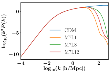
Figure 1: Linear dimensionless matter power spectra generated by CAMB for CDM (blue line) and for the sterile neutrino model with particle mass $m_{SN}=7\,\textrm{keV}$ with three different choices of the lepton asymmetry parameter $L_{6}$, as indicated in the legend (orange, green and red, for $L_{6}=1$, 8 and 12, respectively).

Name	$L\,[{\rm Mpc}/h]$	$N$	Dark matter	UVB	Cosmology
CDM_L128N64	128	$64^{3}$	CDM	no UVB	Viel
CDM_L20N512	20	$512^{3}$
CDM_L20N896	20	$896^{3}$
CDM_L20N1024	20	$1024^{3}$
M7L1	20	$1024^{3}$	$m_{SN}=7\,\textrm{keV},L_{6}=1$	no UVB	Viel
M7L8			$m_{SN}=7\,\textrm{keV},L_{6}=8$
M7L12			$m_{SN}=7\textrm{keV},L_{6}=12$
CDM_Planck_Late	20	$1024^{3}$	CDM	LateR	Planck
CDM_Planck_Early			CDM	EarlyR
M7L12_Planck_Late			$m_{SN}=7\,\textrm{keV},L_{6}=12$	LateR
EAGLE_REF	100 $/h$	$1504^{3}$	CDM	Eagle	Planck

Table 1: Hydrodynamical simulations considered in this work together with corresponding parameters. All simulations were performed specifically for this work, except EAGLE_REF (Schaye et al., 2015). Columns contain from left to right: simulation identifier, co-moving linear extent of the simulated volume ($L$), number of dark matter particles ($N$, there is an equal number of gas particles), type of dark matter (CDM or sterile neutrino WDM with the indicated particle mass, $m_{\rm SN}$ – expressed in natural units – and lepton asymmetry parameter, L₆), ultra-violet background imposed during the simulation (no UVB indicates no UVB was imposed; LateR and EarlyR refer to the UVBs from the LateR and EarlyR reionization models in Oñorbe et al. (2017a), Eagle indicate the standard UVB from (Haardt & Madau, 2001)), choice of cosmological parameters from Table 2, and figure where the particular simulation is used. The gravitational softening length for gas and dark matter is kept constant in co-moving coordinates at 1/30^th of the initial interparticle spacing. All simulations were started from the initial conditions generated by the 2LPTic (Scoccimarro et al., 2012) with the same ‘glass’like particle distribution generated by GADGET-2 (Springel, 2005).

Cosmology	Planck (Ade et al., 2016)	Viel (Viel et al., 2013a)
$\Omega_{0}$	$0.308\pm 0.012$	$0.298$
$\Omega_{\Lambda}$	$0.692\pm 0.012$	$0.702$
$\Omega_{b}h^{2}$	$0.02226\pm 0.00023$	$0.022393$
$h$	$0.6781\pm 0.0092$	$0.7$
$n_{s}$	$0.9677\pm 0.0060$	$0.957$
$\sigma_{8}$	$0.8149\pm 0.0093$	$0.822$

Table 2: Cosmological parameters used in our simulations. Planck cosmology is the conservative choice of TT+lowP+lensing from Ade et al. (2016) (errors represent $68\%$ confidence intervals), while Viel cosmology corresponds to the bestfit model in Viel et al. (2013a).

In this work, we have considered a suite of dedicated cosmological hydrodynamical simulations, and one of the simulations from the Eagle simulation suite. Our dedicated simulation suite has been performed using the simulation code used by Viel et al. (2013b). This code is a modified version of the publicly available gadget-2 TREEPM/SPH code described by Springel (2005); the runs performed are summarised in Table 1. The values of the cosmological parameters used are in Table 2; runs labelled ‘Planck’ use parameters taken from Ade et al. (2016), those labelled ‘Viel’ use parameters taken from Viel et al. (2013a) to allow for a direct comparison with the latter work.

Initial conditions for the runs were generated using the 2LPTic code described by Scoccimarro et al. (2012), for a starting redshift of $z=99$ that guarantees all sampled waves are still in the linear regime. The initial linear power spectrum for the CDM cosmology was obtained with the linear Boltzmann solver CAMB (Lewis et al., 2000). Sterile neutrino dark matter is also modelled as non-interacting massive particles, with the effects of free streaming imprinted in the initial transfer function as computed with the modified CAMB code described by Boyarsky et al. (2009b), using the primordial phase-space distribution functions for sterile neutrinos computed in Laine & Shaposhnikov (2008). Using instead results from the most recent computations (Ghiglieri & Laine, 2015; Venumadhav et al., 2016) would not change our results. We neglect the effects of peculiar velocities of the WDM particles other than the cut-off they introduce in the transfer function. The linear matter power spectra for the different models used in this paper are shown in Fig.1.

Simulations in the same boxes use the same set of random numbers, this allows us to compare Lyman-$\alpha$ forest spectra between CDM and WDM directly (see Fig. 2).

For simulations that include a UVB, we specify the redshift-dependent values of the photoionisation and photoheating rates for hydrogen and helium as input parameters. The version of gadget that we use solves for the radiative heating and cooling of the photoionised gas, given these input rates. Imposing the rates of Oñorbe et al. (2017a) results in a $T-\rho$ relation that is consistent with that of the latter authors. We use the same UVB in the SN cosmology as an example of the reionisation history with a small filtering scale.

SPH (gas) particles are converted to collisionless ‘star’ particles when they reach an overdensity $\rho/\bar{\rho}>1000$ provided their temperature $T<10^{5}$ K. This ‘quick-Lyman-$\alpha$’ set-up reduces run time by avoiding the formation of dense gas clumps with short dynamical times, that would in reality presumably form stars in a galaxy. We can do so, because the impact of forming galaxies on the IGM is thought to be small, particularly at high redshifts and for the low density gas regions to which our analysis is sensitive (Theuns et al., 2002; Viel et al., 2013b).

The simulation from the Eagle simulation suite, EAGLE_REF, has CDM cosmology and UVB as the standard choice from (Haardt & Madau, 2001), further details can be found in (Schaye et al., 2015). Its boxsize and number of particle are respectively $L=100\,{\rm cMpc}$ and to $N_{\rm part}=1504^{3}$, and its resolution is smaller by a factor $\sim 5$ respect to the resolution of our highest resolution simulations. This simulation has been considered for estimating the covariance matrix of the mean FPS.

4.3 Calculation of mock spectra

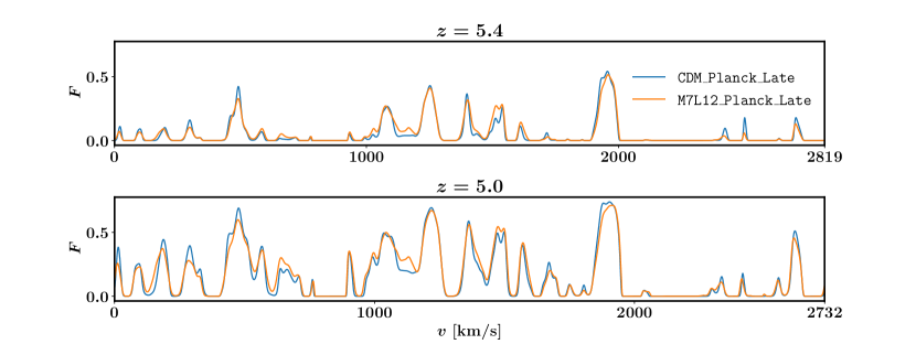
Figure 2: Example mock spectra extracted along the same line of sight in CDM_Planck_Late (blue line) and M7L12_Planck_Late (orange line), simulations at redshifts $5.4$ (top panel) and $5.0$ (bottom panel). The temperature $T_{0}$ of the gas at the mean density at these redshifts is $\sim 7700\textrm{K}$ for both redshifts. Note that a sightline through the full extent of the box corresponds to a different velocity extent at different redshifts. The evolution of the mean transmission is apparent. The CDM and WDM spectra look quite similar, nevertheless on closer inspection it is clear that the CDM spectrum has some sharper features.

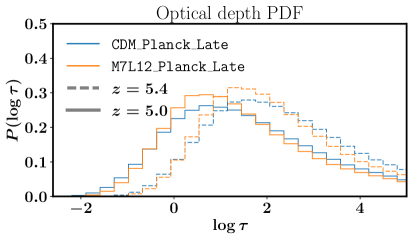
Figure 3: Left panel: probability distribution function of the optical depth per pixel. Right panel: cumulative probability distribution of the effective optical depth, $\tau_{\rm eff}$, measured in chunks of $50\;\textrm{Mpc~{}h}^{-1}$. The CDM_Planck_Late model is plotted in blue, the M7L12_Planck_Late in orange, redshift $z=5.4$ corresponds to dashed lines and $z=5.0$ to full lines.

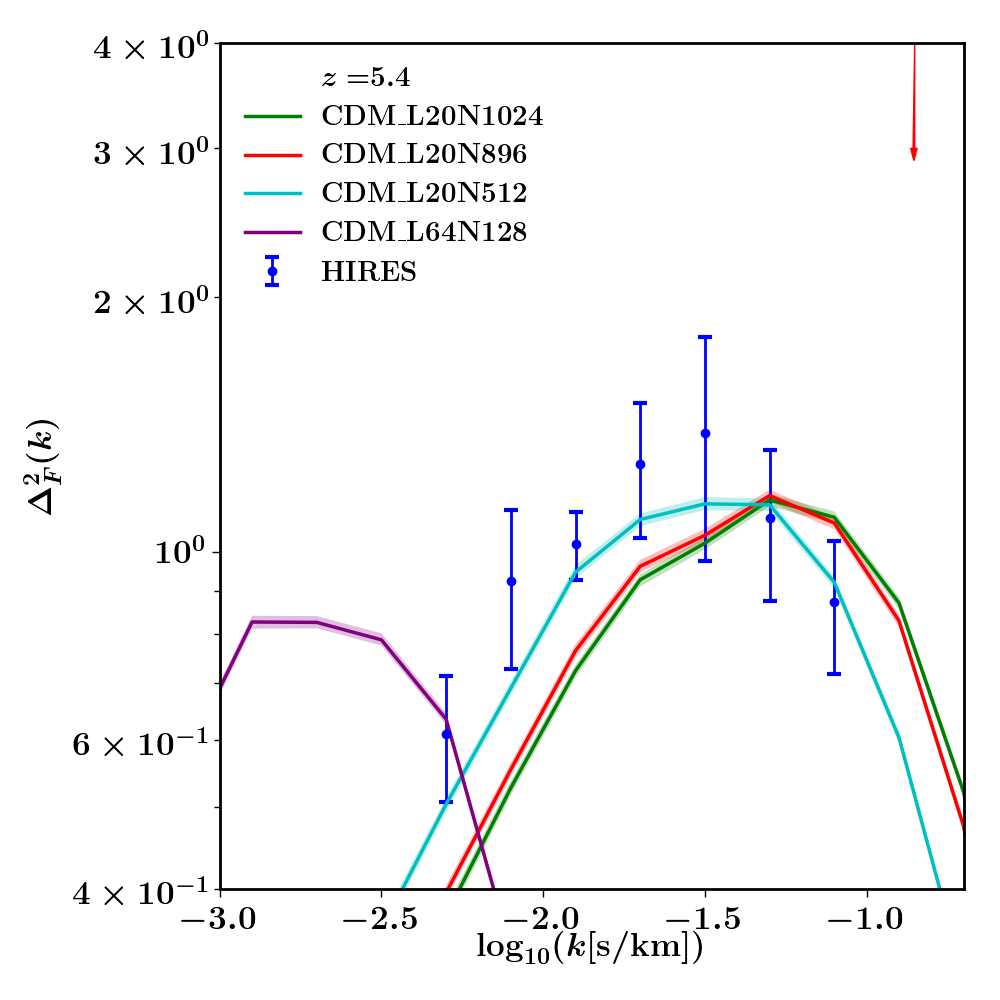
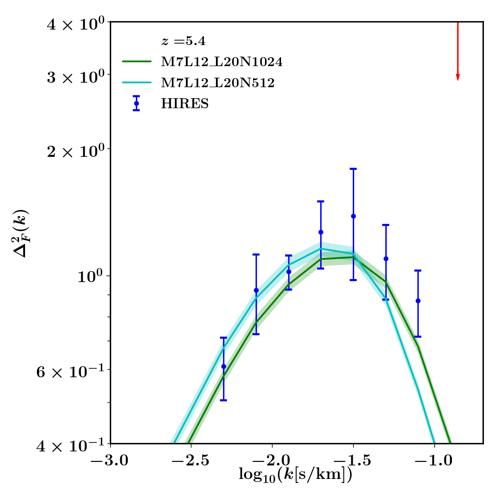
Figure 4: Effect of numerical resolution on the mock FPS for CDM (left panel) and WDM (right panel) of simulations performed without an imposed UVB. Both models are for the imposed power-law $T-\rho$ relation of Eq. (1) with $(T_{0},\gamma)=(25~{}{\rm K},1)$, are scaled to the observed value of the effective optical depth, $\tau_{\rm eff}=3.0$ for $z=5.4$, and mimic the spectral resolution and pixel size of the hires spectrograph on the keck telescope (FWHM=6.7 km s^-1, pixel size=2.1 km sec^-1 (see Section 2) but without adding noise. The data points show the error bars as reported by Viel et al. (2013a) that do not take into account sample variance (see below). The different colours correspond to different numbers of particles $N$, as per the legend. The observed FPS from Viel et al. (2013a) (blue) is plotted to indicate the range of relevant wave numbers. There is a numerical resolution-dependent cut-off in each simulation. Increasing the number of particles, the position of this cut-off shifts to larger $k$ values. In our highest resolution simulations, $N=1024^{3}$ DM and gas particles (green line), the resolution-dependent cutoff is outside the range of scales probed by the Lyman-$\alpha$ data, the corresponding Nyquist scale $k_{\rm max,sim}$ is outside the boundary of the plot. Therefore, we use such resolution in all subsequent simulations. The red arrow shows the scale associated with $k_{\rm max,DM}$. The figure also demonstrates that the simulations considered by Mo et al. (1997) (purple line) lacked the necessary resolution to be used in Desjacques & Nusser (2004).

We compute mock spectra of the simulations using the specwizard code that is based on the method described by Theuns et al. (1998). This involves computing a mock spectrum along a sight line through the simulation box along one of the coordinate axis.

For simulations without a UVB (CDM_L20N1024, M7L12), we first impose a temperature-density relation of the form of Eq. (1) on all gas particles. At the high redshifts that we are considering, the Lyman-$\alpha$ transmission is non-negligible only for sufficiently small overdensities, $\delta\lesssim 1$. We checked explicitly that the effect of cooling at the highest densities is negligible for our analysis. Therefore, one can safely apply the temperature-density relation to the whole range of densities considered, without worrying about it being applicable only in the range $\delta\lesssim 10$ (Hui & Gnedin, 1997).

We use the same post-processing also for simulations which do include a UVB. The rationale behind this is the following. As already mentioned, we use Oñorbe et al. (2017a) ionisation history only as an example of the model with small pressure effects, not as a holistic model. We then vary the $T_{0}$ in post-processing (see Section 5.2 below) and determine the range of admisssible temperatures in CDM and WDM cosmologies. We verify a posteriori that the actual temperature predicted by the LateR model lies within the range of admissible temperatures.

Given $T$ and $\rho$ of each particle, we compute the neutral fraction $x$ using the interpolation tables from Wiersma et al. (2009), which assume photoionisation equilibrium,

$${dn_{\text{H\,{1}}}\over dt}=-\Gamma_{\text{H\,{1}}}n_{\text{H\,{1}}}-\Gamma_{c}\,n_{e}\,n_{\text{H\,{1}}}+\alpha(T)\,n_{e}\,n_{\text{H\,{ii}}}=0\,.$$ (14)

Here the terms from left to right are photoionisation by the imposed UVB, collisional ionisation, and recombination (with $\alpha(T)$ the temperature-dependent case-A recombination coefficient); $n_{e}$ is the electron density; the photoionisation rate is that described by Haardt & Madau (2001).

We then interpolate the temperature, density, and peculiar velocity to the sight line in bins of $\Delta v=1$ km s^-1 using the Gaussian method described by Altay & Theuns (2013). We verified that this spectral resolution is high enough to give converged results. We then compute the optical depth as function of wavelength, $\tau(v)$, thus accounting for Doppler broadening and the effects of peculiar velocities.

To allow for a fair comparison to the observed spectra, we convolve the mock spectra with a Gaussian to mimic the effect of the line-spread function, and rebin to the observed pixel size with parameters as described in Section 2. The Gaussian white noise has a uniform relative Standard Deviation of $\sigma=0.066$, corresponding to a signal to noise ratio of $S/N=15$ per pixel at the continuum level, following Viel et al. (2013a). Further details on the application of noise to mock spectra and comparison with previous work are given in Appendix C. We calculate a set of such spectra for the snapshot at redshifts $z=5$, and $z=5.4$.

After repeating this procedure for ${\cal N}=10^{3}$ sight lines, we compute the mean transmission, $\langle F\rangle=\langle\exp(-\tau)\rangle$ and scale the optical depth so that the ensemble of mock spectra reproduces the observed value of $\langle F\rangle$ discussed in Section 2.

We compare spectra along the same sight line for the CDM and the M7L12_Planck_Late models in Fig. 2 (blue and orange curves, respectively), at redshifts $z=5.4$ (top panel), and $z=5.0$ (bottom panel); the temperature and thermal history are the same for both models. The Lyman-$\alpha$ spectra look very similar in these models, although it can be seen that the CDM model has some sharper features.

The probability distribution function (PDF) of the optical depth is compared between these two models in Fig. 3.

4.4 Numerical convergence

Before comparing the mock FPS to the observed FPS, we investigate to what extent the mock FPS is converged, both in terms of resolution and box size; the latter discussion can be found in Appendix A. The gas temperature in our simulations that were performed without an imposed UVB is very low, and the gas distribution itself is not numerically converged at any of our resolutions. The effect of that on the FPS is shown in Fig. 4. For an imposed $T-\rho$ relation with $(T_{0},\gamma)=(25{\rm K},1)$, the CDM FPS does show a cut-off at small scales, but the value of $k_{\rm max}$ increases with increasing particle count, $N$. The value of $k_{\rm max}$ for $N=896^{3}$ and $N=1024^{3}$ is nearly identical (see Fig. 4). We run our main analysis with the box size $L=20\,{\rm Mpc/}h$ and $N=1024^{3}$ of both DM and gas particles, the corresponding scale $k_{\rm max,sim}$ is therefore much larger than $k_{s}$.

Our resolution is higher than used previously (Viel et al., 2013a) as the latter work was interested in hotter thermal histories – IGM with the temperature $T_{0}\sim 10000-20000\,{\rm K}$ with a non-negligible thermal smoothing. Note that Viel et al. (2013a) also recongnized that $N=512^{3}$ with $L=20$ Mpc/$h$ resolution is insufficient, but they applied a correcting factor to all power spectra. This factor was calibrated with a single simulation with $N=896^{3},L=20~{}{\rm Mpc/}h$. We instead rely on the intrinsic convergence of our simulations in the range of available data.

5 The flux power spectrum in CDM and WDM

5.1 Varying the cut-off in the FPS

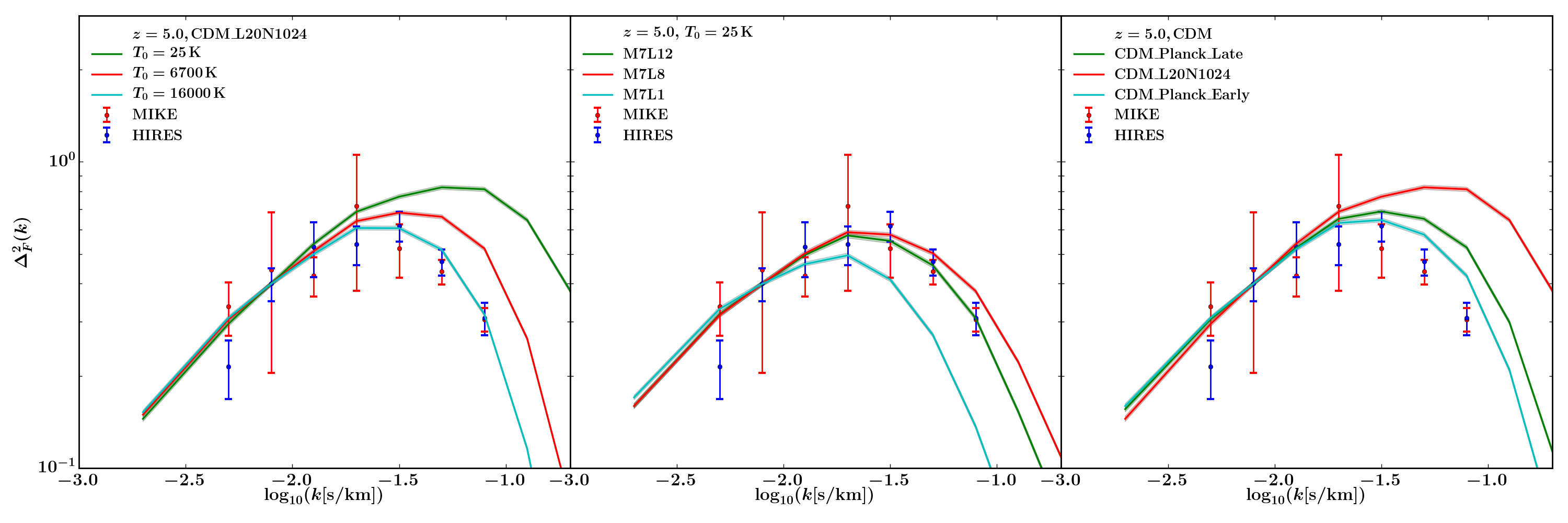
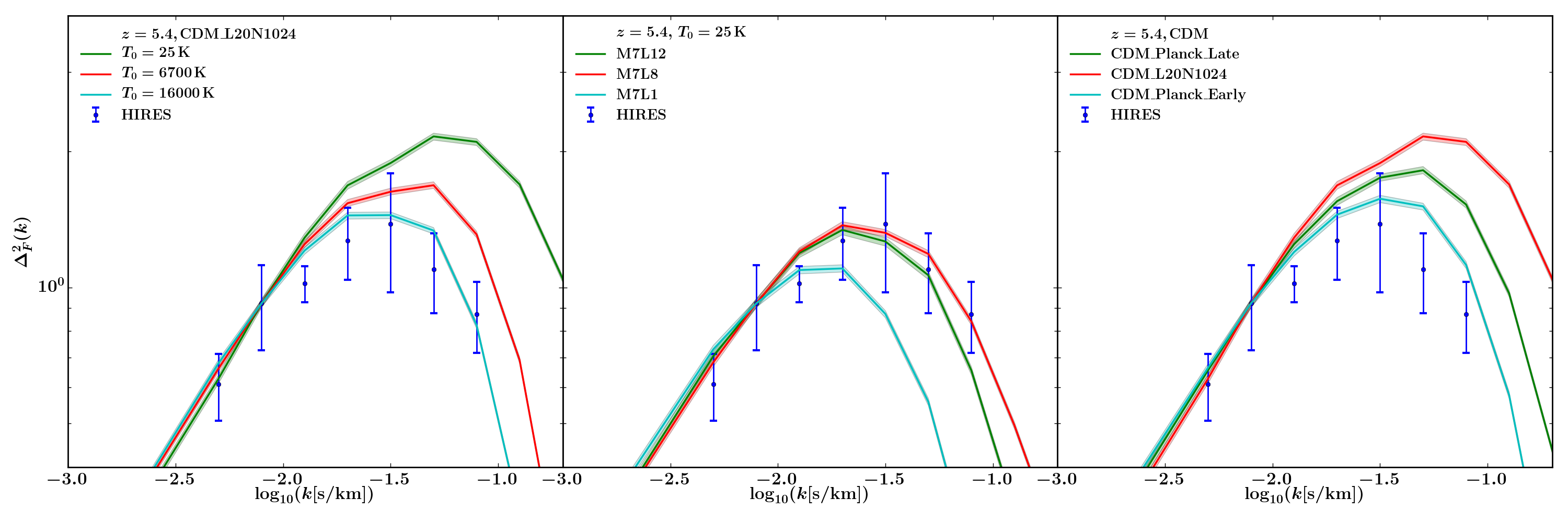
Figure 5: The cut-off in the mock flux power spectrum for various models, compared to the hires (blue dots with error bars) and mike data (red dots with error bars) at redshifts $z=5.0$ (upper panels) and $z=5.4$ (lower panels). For illustration purposes, we have scaled the amplitudes of the mock FPS in all cases such that it agrees with the hires value for the second point from the left, as a result different FPS in the same panel have different $\tau_{\rm eff}$. Left panels: model CDM_L20N1024 with three imposed temperature-density relations for $T_{0}=16000$ K, 6700 K, and 25 K (cyan, red and green curves, respectively). Doppler broadening introduces a cut-off in the FPS that resembles the observed cut-off, for temperatures $\sim 2\times 10^{4}$ K. Middle panels: WDM simulations WDM_L1, WDM_L8 and WDM_L12 (cyan, red and green curves, respectively), with negligible Doppler broadening, $T_{0}=25$ K. DM free-streaming alone produces a cut-off in the FPS that resembles the observed cut-off for $L_{6}=8$ and $12$. Right panels: CDM simulations CDM_L20N1024 without pressure effects (red) compared to the simulations where the pressure effects are modeled using the reionisation model of Oñorbe et al. (2017a) : late reionisation model in CDM_Planck_Late (green curve) and early reionisation model in CDM_Planck_Early (cyan curve). To illustrate the effects of pressure history alone, the Doppler broadening of the lines is reduced by assigning the uniform temperature of $T_{0}=25$ K in post-processing.

We begin this section with illustrating how Doppler broadening, WDM free-streaming, and pressure smoothing, as quantified by $\lambda_{b}$, $\lambda_{\rm DM}$ and $\lambda_{p}$, respectively, all lead to cut-off in mock FPS. Our results are summarized in Figure 5.

Doppler broadening introduces a cut-off in the FPS, which in the case of CDM, resembles the observed cut-off for an imposed power-law temperature-density relation (1), with $T_{0}\sim 2\times 10^{4}$ K and $\gamma=1$, as shown in the left panels of Fig. 5, see also Oñorbe et al. (2017b).

Even in the absence of Doppler broadening, WDM free-streaming introduces a cut-off in the FPS which resembles the observed cut-off for sufficiently ‘cold’ WDM models. Those with Lepton asymmetry parameter $L_{6}=8$ or 12, middle panel of Fig. 5, appear consistent with the hires data. (We will perform a more detailed statistical comparison below.)

Finally the right panel in Fig. 5 shows the effects of pressure smoothing on the cut-off in the CDM case.

5.2 Comparison between mock and observer FPS cut-off

We have varied the parameters of our models to obtain the best fit to the cut-off in the FPS by performing a $\chi^{2}$ analysis. To this end we use the evolution of the photo-ionisation and photo-heating rate of the LateR reionization model of Oñorbe et al. (2017a), impose the temperature-density relation with $\gamma=1$ in post-processing, and scale the simulated mean transmission to a range of values characterised by $\tau_{\rm eff}\equiv-\log\langle F\rangle$. As described in Section 4.3, we convolve the mock spectra with a Gaussian to mimic instrumental broadening, rebin to the pixel size of the spectrograph, and add Gaussian noise with standard deviation independent of wavelength and flux, corresponding to a signal to noise of 15 at the continuum level. We compute a grid of mock FPS, varying $T_{0}$ and $\tau_{\rm eff}$ for CDM and WDM models. We compare the mock FPS to the observed FPS at redshifts $z=5$ and $z=5.4$. When doing the comparison we take into account that the scattering between different realisations is large due to the small size of QSO samples (see Section 2 for details). We take into account the sample variance by computing the $\chi^{2}$ of a model using the covariance matrix computed from EAGLE_REF (as the boxsize of our reference simulation is not large enough to compute the covariance matrix). The rationale behind choosing EAGLE_REF was its large boxsize. the total length of the lines-of-sight in simulation was chosen equal to the total length of the observed QSO sample for each redshift range. Although EAGLE simulations does not have sufficient resolution at the smallest scales, we expect that the covariance is reproduced correctly.

The resulting contours for $68\%$ and $95\%$ confidence levels for hires data are shown in Fig. 6. In Table 3 we have compiled the values of the $\chi^{2}$ for the best-fitting models.

Table 3: Values of $\chi^{2}$ for the best-fitting models shown in Figure 6. The number of dof is 5.

model	$z$	$\chi^{2}$
CDM_Planck_Late	5.0	2.20
	5.4	3.25
M7L12_Planck_Late	5.0	3.44
	5.4	2.85

For completeness, in Appendix E we have shown the same analysis for the HIRES data-sets at the redshift intervals centered on $z=4.2$ and $z=4.6$, that have already been discussed in (Viel et al., 2013a).

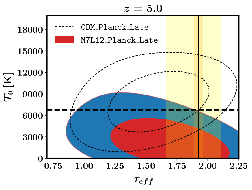
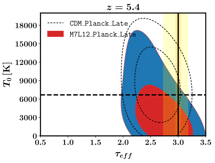
Figure 6: Confidence levels of mock FPS compared to the observed FPS of hires for redshifts $z=5$ (left) and $z=5.4$ (right). We vary the temperature at the mean density, $T_{0}$, keeping $\gamma=1$, and the value of the effective optical depth $\tau_{\rm eff}$. Solid lines and colour shaded areas correspond to $68\%$ and $95\%$ uncertainty intervals for the $m_{\rm SN}=7\,{\rm keV}$ and $L_{6}=12$ WDM model, dashed lines are the same for the CDM model. Both models used the late reionisation model LateR from Oñorbe et al. (2017a). The contours take into account both hires error bars as reported by Viel et al. (2013a) and additional errors due to finite number of quasars in the dataset. The black solid vertical line is the directly estimated $\tau_{\rm eff}$ as reported in Viel et al. (2013a). The horizontal line shows the value of $T_{0}$ as obtained in simulations with LateR UVB and without post-processing. It is in full agreement with the results of Oñorbe et al. (2017a). The systematic uncertainty on $\tau_{\rm eff}$ coming from the sample variance is estimated to be $\sim 10\%$, and we have indicated the resulting uncertainty on $\tau_{\rm eff}$ with the orange shade. The uncertainty on $\langle F\rangle$ due to continuum fitting is reported to be at the level $\sim 20\%$, and we have indicated the resulting uncertainty on $\tau_{\rm eff}$ with the yellow shade.

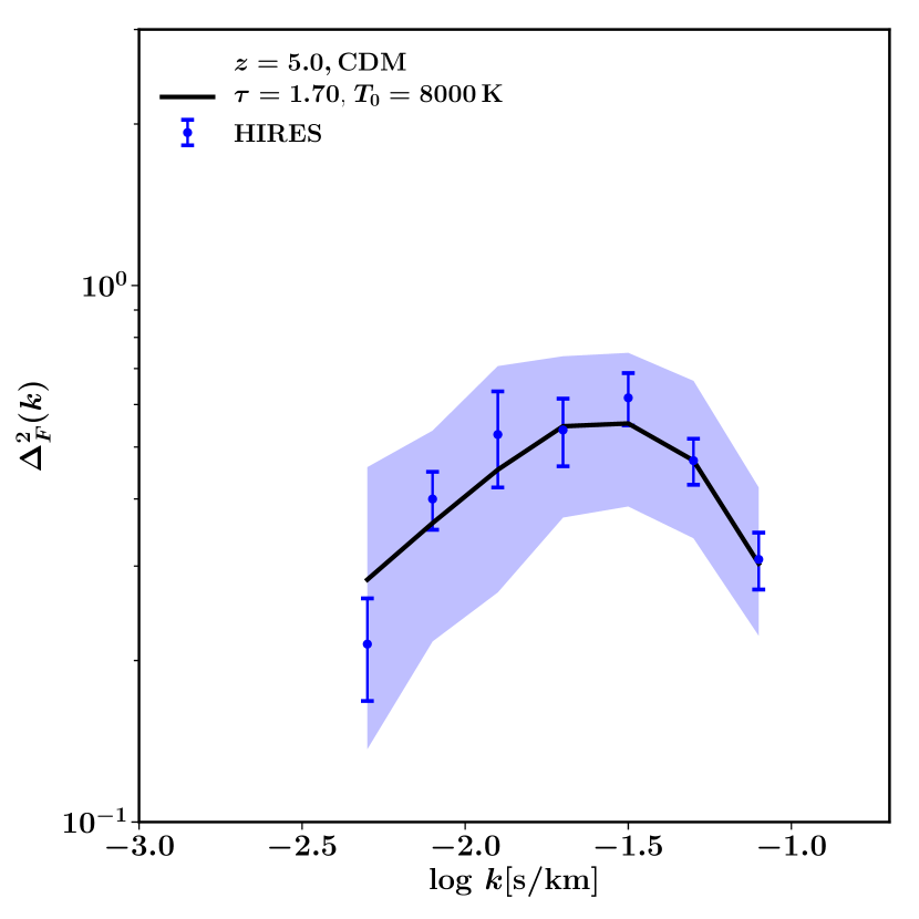
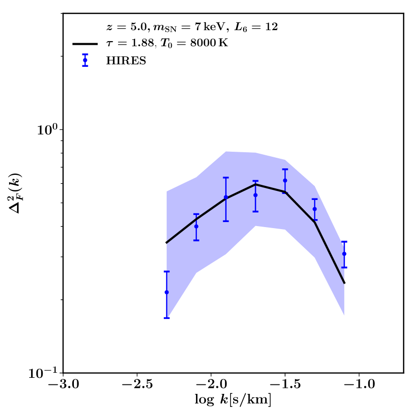
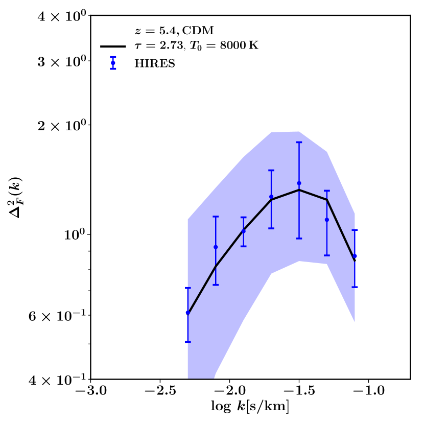
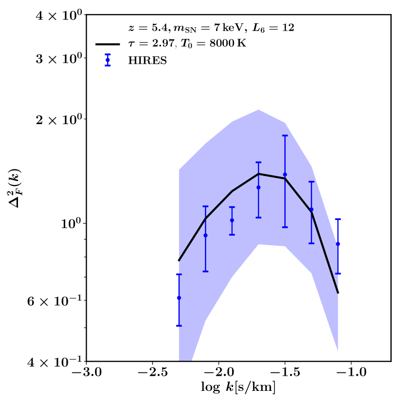
Figure 7: Examples of CDM and WDM models with realistic thermal histories, consistent with the high-resolution Lyman-$\alpha$ data. For both models we choose $T_{0}=8000$ K as predicted by our simulations with LateR UVB from Oñorbe et al. (2017a). The observed FPS inferred from hires is plotted as blue symbols with error bars as reported by Viel et al. (2013a). One should keep in mind that the data points are correlated and therefore do not fluctuate independently. Shaded regions around the model show the variance due to different realisations of mock FPS (with the total length of the lines-of-sight in simulations equal to the length of observed spectra in the dataset for each redshift interval). The mock spectra have best-fit effective optical depth $\tau_{\rm eff}\equiv-\log\left<F\right>$ for the fixed uniform temperature $T$ imposed in post-processing. Top panels are for redshift $z=5$ and bottom panels – for redshift $z=5.4$ for CDM (left panels) and M7L12 SN model (right panels). The simulations are CDM_Planck_Late (left panels) and M7L12_Planck_Late (right panels).

As can be seen already from Fig. 5 (central panel), the WDM model M7L12 has the FPS suppression due to the free-streaming that is consistent with the data. Therefore when varying $T_{0}$ in post-processing, WDM prefers temperatures with the scale $\lambda_{b}\ll\lambda_{\rm DM}$, see Fig. 6. At the same time, our simulation M7L12_Planck_Late predicts a temperature $T_{0}^{\rm sim}\simeq 7700$ K at both redshifts $5.0$ and $5.4$ (also in agreement with findings of Oñorbe et al. (2017a)) . From Fig. 6 we see that the hires data is consistent with $T_{0}^{\rm sim}$ within its $95\%$ confidence interval. Thus our procedure of post-processing is self-consistent – the temperature predicted by the simulations is consistent with the data. We show in Fig. 7 WDM model with this $T_{0}$ K as an example of a model with realistic thermal history, compatible with the data A proper analysis, that varies all three scales: $\lambda_{p}$, $\lambda_{b}$ and $\lambda_{\rm DM}$ will be done elsewhere.

6 Discussion

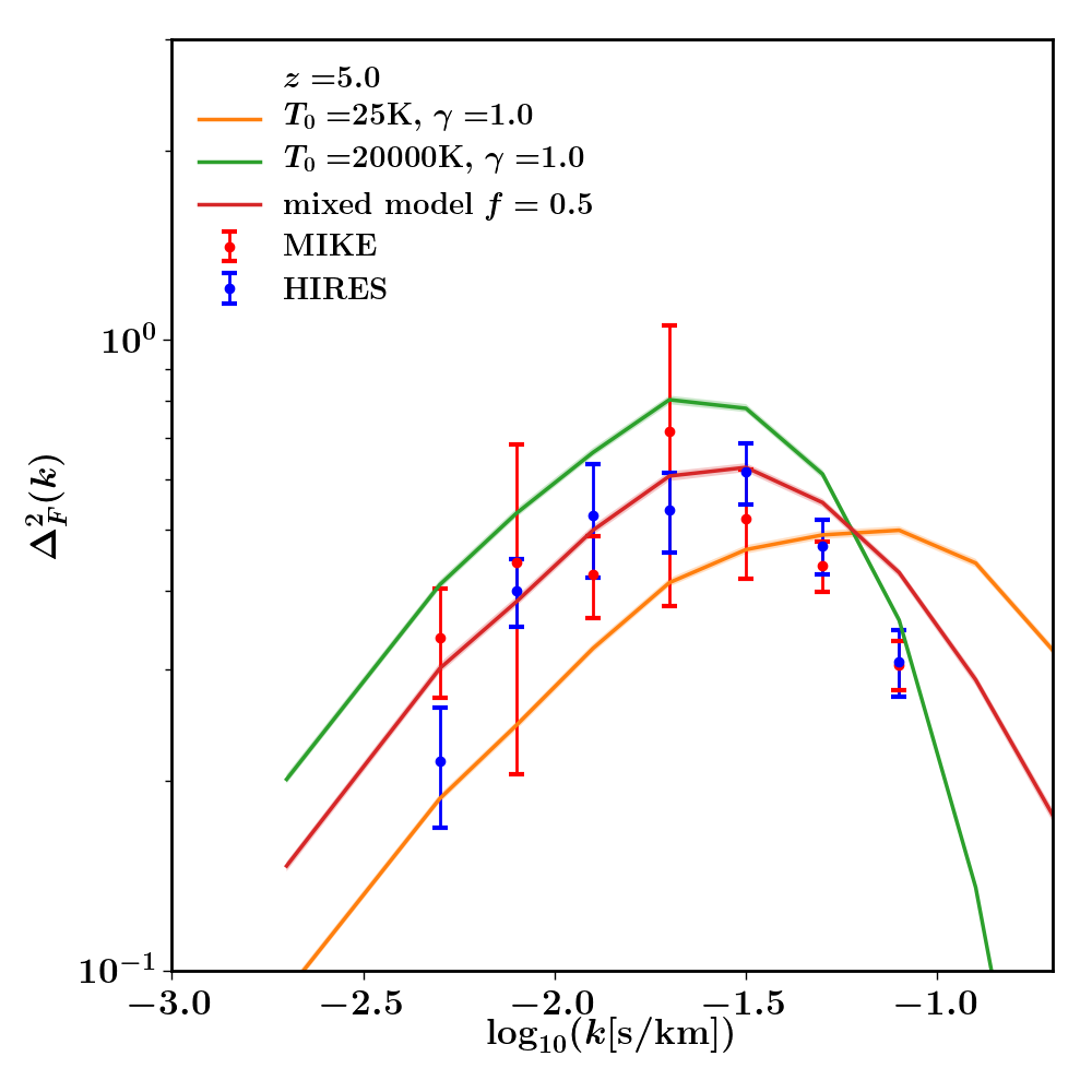
Figure 8: The effect of temperature fluctuations on FPS, for the case that bubbles are much larger than our simulated volume at $z=5.0$. This case corresponds to a mixing fraction $f=0.5$. For reference, we have drawn the data points of the MIKE and HIRES samples.

In the previous section we demonstrated that a WDM model with $m_{\rm SN}c^{2}=7$ keV and Lepton asymmetry parameter $L_{6}\sim 12$ fits the Lyman-$\alpha$ flux power spectrum at redshifts $z=5$ and 5.4 as well as a CDM model, provided that the Doppler broadening $\lambda_{b}$ and the pressure broadening $\lambda_{p}$ are both sufficiently small. What is currently known about these $\lambda$’s?

Since $\lambda_{b}$ is set by $T_{0}$, we start by examining limits on the IGM temperature. When neutral gas is overrun with an ionisation front during reionisation, the difference between the energy of the ionising photon and the binding energy of H i, $\Delta E=h\nu-13.6~{}{\rm eV}$, heats the gas. In the case of H ii regions, gas will also cool through line excitation and collisional cooling, resulting in a temperature immediately following reionisation of $T_{0,{\rm reion}}\leqslant 1.5\times 10^{4}$ K (Miralda-Escude & Ostriker, 1990; Miralda-Escudé & Rees, 1994). In the case of reionisation, the low density of the IGM suppresses such in-front cooling, and the numerical calculations of McQuinn (2012) suggest $T_{0,{\rm reion}}=1-4\times 10^{4}$ K, depending on the spectral slope of the ionising radiation. Following reionisation, the IGM cools adiabatically while being photoheated, preserving some memory of its reionisation history (Theuns et al., 2002; Hui & Haiman, 2003). Therefore the value of $T_{0}$ at $z=5.4$ is set by $T_{0,{\rm reion}}$, the redshift $z_{\rm reion}$ when reionisation happened, and the shape of the ionising radiation that photoheats the gas subsequently. For $T_{0}$ to be sufficiently low then requires that $T_{0,{\rm reion}}$ is low, that $z_{\rm reion}\gg 5.4$, and that the ionising radiation is sufficiently soft.

Taking $z_{\rm reion}=7.82$ from Planck Collaboration et al. (2018) and $T_{0,{\rm reion}}=1.5\times 10^{4}$ K yields a guesstimate for the lower limit of $T_{0}\sim 0.8\times 10^{4}$ K at $z=5.4$, consistent with the value of $T_{0}\sim 10^{4}~{}$K suggested by Oñorbe et al. (2017b) that we used in the previous section. There is now good evidence that He ii reionised at $z~{}\sim 3.5$, much later than H i and He i (Jakobsen et al., 1994; Schaye et al., 2000; La Plante et al., 2017; Syphers & Shull, 2014), as the ionising background hardens due the increased contribution from quasars. This suggests that the ionising background during reionisation was unable to ionise He ii significantly and hence was relatively soft. So conditions for low $T_{0}$ seem mostly satisfied.

However the FPS also depends on the slope $\gamma$ of the temperature-density relation, not just $T_{0}$. As gas is impulsively heated during reionisation, the heat input per hydrogen atom is mostly independent of density, driving $\gamma\rightarrow 1$. The heating rate then drops as the gas becomes ionised, but more so at low density than at high density. This steepens the TDR asymptotically to $\gamma-1=1/(1+0.7)\sim 0.6$, with the factor 0.7 resulting from the temperature dependence of the case-A H ii recombination coefficient (Theuns et al., 1998; Upton Sanderbeck et al., 2016). The characteristic time-scale for approaching the asymptotic value is of the order of the Hubble time. If reionisation indeed happens late, $z\sim 7.5$, then we would expect $1<\gamma<1.6$.

Observationally, the IGM temperature is constrained to be at the level $T_{0}\gtrsim 8000$ K at $z\lesssim 4.6$ (Schaye et al., 2000; McDonald et al., 2001; Lidz et al., 2010; Becker et al., 2011) (see e.g. Upton Sanderbeck et al. (2016) for a recent discussion). At $z\approx 6.0$ there is a single measurement in the near zone of a quasar that yields $5000<T_{0}<10000$ K (68% CL, Bolton et al. (2012)). Fundamentally, all of the techniques used to infer $T_{0}$ observationally are based on identifying and computing the statistics of sharp features in Lyman-$\alpha$ forest spectra, and comparing these to simulated spectra. This implies that the $T_{0}$ inferred implicitly depends on $\lambda_{\rm DM}$.

Combining the theoretical prejudice and the measurements, we conclude that a value of $T_{0}\sim 8000$ K or even colder at redshifts around 5 is not unreasonable and definitely not ruled out. Using Eq. (8), such a value of $T_{0}$ yields $k_{{\rm max},b}=0.12$ (km s^-1)^-1.

What do we know about $\lambda_{p}$? From a theoretical perspective, this ‘Jeans’ or ‘pressure broadening’ results from Hubble expansion over the finite extent of the absorbing filament (Garzilli et al., 2015). In the linear approximation, this results in a value of $\lambda_{p}$ that is in general smaller than the Jeans length $\lambda_{J}$ because gas needs to physically expand away from the much thinner dark matter filaments before it reaches the final filament width Gnedin & Hui (1998). In the special case but not unrealistic case where $T_{0}\approx 0$ before reionisation and a constant after reionisation, Gnedin & Hui (1998) find

$$\left({\lambda_{p}\over\lambda_{J}}\right)^{2}={3\over 10}\left[1+4\left({1+z\over 1+z_{\rm reion}}\right)^{5/2}-5\left({1+z\over 1+z_{\rm reion}}\right)^{2}\right]\,.$$ (15)

Taking again $z_{\rm reion}=7.82$ yields $\lambda_{p}=(0.3-0.2)\lambda_{J}$ at redshift $z=5$ and 5.4, respectively, or in terms of the cut-off in the FPS using Eq. (10), $k_{{\rm max},p}=0.3-0.4$ (km s^-1)^-1.

Comparing these estimates of $\lambda_{b}=1/k_{{\rm max},b}\sim 8~{}{\rm km~{}s}^{-1}$ and $\lambda_{p}=1/k_{{\rm max},p}\sim 3~{}{\rm km~{}s}^{-1}$, it is not surprising that WDM free-streaming with $\lambda_{\rm DM}\sim 10~{}{\rm km~{}s}^{-1}$ dominates the cut-off in the FPS in the WDM case. Since this is also close to the observed cut-off scale show why such a WDM model is consistent with the data. We note in passing that a small value of $\lambda_{b}$ favours reionisation to be early, whereas a small value of $\lambda_{p}/\lambda_{J}$ favours reionisation to be late. The current value of $z_{\rm reion}\approx 7.8$ happens to be a good compromise between the two.

The plausible patchiness of reionisation introduces complications. For example the large-scale amplitude of the FPS may be more a measure of the scale and amplitude of temperature fluctuations or of fluctuations in the mean neutral fraction, rather than being solely due to density fluctuations that we simulate. If that were the case, then our simulations should not match the measured FPS on large-scales, since we have not included these effects (see e.g. Becker et al. (2015)). Furthermore, what is the meaning of $\lambda_{b}$ or $\lambda_{p}$ in such a scenario, where these quantities are likely to vary spatially? Matching the cut-off in the FPS might pick-out in particular those regions where both $\lambda_{b}$ and $\lambda_{p}$ are unusually small.

To illustrate the effect of fluctuations on the FPS, we contrast the FPS of two sets of mock spectra with an imposed temperature-density relation with different values of $T_{0}$: 25 K (i.e. negligible Doppler broadening and $T_{0}=2\times 10^{4}$ K in Fig. 8, as well as a mock sample that uses half of the spectra from each of the two models. The FPS for the single-temperature models are normalized to have the same mean effective optical depth, $\tau_{\rm eff}=2.0$, the mixed-temperature model is computed from the two normalized single-temperature models, and it is not normalized further. We find that in the mixed model the FPS is intermediate between the FPS of the hot and cold models. Hence, if the hot model represents the recently reionized regions in the IGM and the cold model the patches that were reionized previously and then cooled down, the mixed model looks like a model that is colder than the regions in the IGM that were reionized more recently.

Fig. 8 illustrates that fluctuations essentially decouple the behaviour of the FPS at large and small scales. If this is the case of the real IGM, then what we determine to be $T_{0}$ from fitting the cut-off does not correspond to either the hot or the cold temperature. We leave a more detailed investigation of patchiness on the FPS and how that impacts on constraints on $\lambda_{\rm DM}$ to future work.

7 Conclusions

The power spectrum of the transmission in the Lyman-$\alpha$ forest (the flux power spectrum, FPS), exhibits a suppression of power on scales smaller than $\lambda_{\rm min}=1/k_{\rm max}\sim 30~{}{\rm km~{}s}^{-1}$. Several physical effects may contribute to this observed cut-off: (i) Doppler broadening resulting from the finite temperature $T_{0}$ of the intergalactic medium (IGM), (ii) Jeans smoothing due to the finite pressure of the gas, and (iii) dark matter free streaming; these suppress power below scales $\lambda_{b}$, $\lambda_{p}$ and $\lambda_{\rm DM}$, respectively. We have shown in Section 3 that, when $\lambda$ is expressed in velocity units, $\lambda_{b}$ and $\lambda_{p}$ are independent of redshift $z$ for a given value of $T_{0}$, whereas $\lambda_{\rm DM}\propto(1+z)^{1/2}$. This means that any smoothing of the density field due to warm dark matter (WDM) free-streaming will be most easily observable at high-redshift, and the observed FPS may provide constraints on the nature of the dark matter (Viel et al., 2013a; Iršič et al., 2017a; Iršič et al., 2017b; Murgia et al., 2018), and possible be a ‘WDM smoking gun’.

In this paper we tried to answer two questions:

• Does the observed cut-off in the FPS favour cold or warm dark matter, or can both models provide acceptabale fits to the existing data?

• Are the WDM models with large $\lambda_{\rm DM}$ that were previously excluded allowed if one considers a less restrictive thermal history?

To answer these questions we run a set of cosmological hydrodynamical simulations at very high resolution, varying $\lambda_{b}$, $\lambda_{p}$ and $\lambda_{\rm DM}$ independently. We then compute mock spectra that mimic observational limitations (noise, finite spectral resolution and finite sample size), and compare the mock FPS to the observed FPS.

We demonstrate that all three effects (i.e. Doppler broadening, Jeans smoothing and DM free-streaming) yield a cut-off in the FPS that resembles the observed cut-off. Of course in reality all three effects will contribute at some level. In particular, Doppler broadening and Jeans smoothing both depend on the temperature $T_{0}$ of the IGM, and so always work together.

To answer the two questions posed above, we have tried to fit the observed FPS at redshifts $z=5$ and 5.4 with (i) a CDM model (which has $\lambda_{\rm DM}=0$), varying $T_{0}$ and the thermal history, and (ii) the particular case of a resonantly produced sterile neutrino WDM model (characterised by the mass of the particle, $m_{\rm DM}c^{2}=7$ keV, and the Lepton asymmetry parameter $L_{6}$, Boyarsky et al. (2009b)), varying $L_{6}$, $T_{0}$ and the thermal history.

In addition to motivations based on particle physics (see e.g. Boyarsky et al. (2018) our particular choice of WDM particle is motivated by the fact that (i) its decay may have been observed as a 3.5 keV X-ray line in galaxies and clusters of galaxies (Boyarsky et al., 2014; Bulbul et al., 2014; Boyarsky et al., 2015), (ii) it produces galactic (sub)structures compatible with observations (Lovell et al., 2016, 2017), and (iii) it is apparantly ruled out by the observed FPS  (Baur et al., 2017).

Fig. 7 shows how the hires data is compatible with CDM and SN cosmologies if we choose relatively late reionisation model (LateR of Oñorbe et al. (2017b)) so that $\lambda_{p}$ is small and $T_{0}\approx 7-8000$ K as predicted by this model. Both the assumed late reionisation redshift, and the relatively low value of $T_{0}$, are reasonable and consistent with expectations and previous work, as we discuss in detail in the Discussion section. Crucially, a WDM model with $L_{6}=12$ and the same late redshift of reionisation also provides an acceptable fit to the data, provided $T_{0}\leqslant 7000$ K. With such a low value of $\lambda_{b}$ and $\lambda_{p}$, the FPS cut-off is mostly due to WDM free streaming.

From this comparison we conclude that the observed suppression in the FPS can be explained by thermal effects in CDM model but also by the free-streaming in a WDM model: current data do not strongly favour either possibility. We also find a reasonable fit for a WDM model that was previously ruled out by Viel et al. (2013a) and (Iršič et al., 2017a; Iršič et al., 2017b; Murgia et al., 2018). Our present analysis differs in a number of ways:

1. We vary the thermal history of the IGM within the allowed observational limits as discussed by Oñorbe et al. (2017a, b). The previous works modeled the UVB according to Haardt & Madau (2001). The latter scenario is known to reionise the Universe too early with respect to current observations (Oñorbe et al., 2017a), plausibly overestimating $\lambda_{p}$.

2. We did not use any assumptions about the evolution $T_{0}(z)$ but inferred ranges of $T_{0}$ at $z=5.0$ and $z=5.4$ based on theoretical considerations and limits inferred from the Lyman-$\alpha$ data (see also Garzilli et al. (2017)).

We also reconsidered the impact of peculiar velocities (‘redshift space distortions’), which were claimed to affect the appearance of a cut-off at the smallest scales (Desjacques & Nusser, 2004), but found these not to be important at the much higher resolution of our simulations.

We also demonstrated that spatial fluctuations in temperature, which are expected to be present close to reionisation, may dramatically affect the FPS. Spatial variations in $T_{0}$ can dramatically increase the amplitude of the FPS at the scale of the imposed fluctuations, effectively decoupling the large-scale and small-scale FPS. Unfortunately this means that a model without fluctuations in $T_{0}$ will yield incorrect constraints on parameters if such fluctuations are present in the data. Interestingly, the nuisance caused by fluctuations in $T_{0}$ may actually be rather helpful if the cut-off in the FPS is in fact due to WDM, since in that case there would be no spatial fluctuations in the location of the cut-off - and the evolution with redshift of the cut-off would follow $\lambda_{\rm DM}\propto(1+z)^{1/2}$.

Moving away from Lyman-$\alpha$ and studying the small-scale Universe in the H i 21-cm line during the ‘Dark Ages’ (Pritchard & Loeb, 2012) instead is currently almost science fiction, but ultimately may be the most convincing way of determining once and for all whether most of the dark matter in the Universe is warm or cold.

Appendix A Convergence of the simulations in box-size

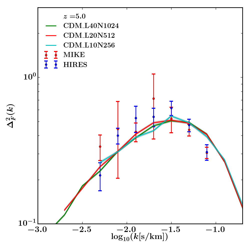
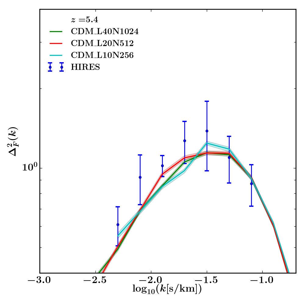
Figure 9: Study of the box-size needed in the numerical simulations to resolve the smallest scales probed by the HIRES and MIKE data samples. We show the FPS at $z=5.0$ and $z=5.4$ for three simulations without UVB and different box-sizes, yet same resolution. We have imposed a uniform temperature $T=25\,{\rm K}$ in the post-processing of the spectra. We have applied the resolution of the HIRES spectrograph to the spectra, but we have excluded the effect of noise on the spectra. The FPS are normalized to the nominal observed optical depth of the observed spectra. The red solid line has a box-size $L=10\,{\rm Mpc}/h$, the green solid line $L=20\,{\rm Mpc}/h$, and the orange solid line $L=40\,{\rm Mpc/h}$. The FPS for the case of $L=10$, $L=20\,{\rm Mpc}/h$, and $L=40\,{\rm Mpc}/h$ agree with each other.

We have investigated the convergence of the FPS in box-size of the simulation with constant resolution. In section 4.4 we have concluded that we need at least a number of particles $N=1024^{3}$ and a boxsize $L=20\,{\rm Mpc}/h$ to resolve the smallest scales reached by the data. Because we do not have the computing power to run a simulation with $L=40\,{\rm Mpc}/h$ with this maximal resolution, we consider three simulations with $L=10,20,40\,{\rm Mpc}/h$ and half the resolution. In this limit, we show in Figure 9 that the $L=20\,{\rm Mpc/h}$ is sufficient to resolve the scales we intend to study.

Appendix B Effect of peculiar velocities on Flux Power Spectrum

In CDM cosmologies the real-space MPS, $\Delta^{2}_{r,3d}(k)$, is a monotonically increasing function of $k$. However, in velocity space over which the FPS observable is built, an additional effect – the redshift space distortions (RSD) – affect the shape (Kaiser, 1987; Kaiser & Peacock, 1991; McGill, 1990; Scoccimarro, 2004). RSD may erase small-scale power in the FPS because peculiar velocities of baryons are non-zero.

At linear level MPS in velocity space is related to real space by:

$$\Delta^{2}_{s,3d}(k)=\Delta^{2}_{r,3d}(k)(1+\beta(\vec{k}\cdot\hat{z})^{2})^{2}$$ (16)

where $\hat{z}$ is the direction of observation and constant $\beta$ for linear scales is given by expression $\delta_{r}=-\beta^{-1}\vec{\nabla}\cdot\vec{v}$ (Kaiser, 1987).

Real-space MPS projected along the line of sight is given by:

$$\Delta^{2}_{r,1d}(q) =\frac{q}{2\pi}\int d^{2}k_{\perp}\frac{\Delta^{2}_{r,3d}(q,k_{\perp})}{\left(q^{2}+k_{\perp}^{2}\right)^{3/2}}$$ (17)

$$=q\int_{q}^{\infty}\frac{dk}{k^{2}}\Delta^{2}_{r,3d}(k)$$ (18)

Clearly, in CDM linear $\Delta^{2}_{r,1d}(k)$ remains a monotonic function of $k$. Non-linear MPS experiences additional growth at small scales, therefore $\Delta^{2}_{r,1d}(k)$ does not exhibit a cutoff also at non-linear level.

Beyond the linear regime it is not possible to compute analytically the effect of RSD on the MPS. Desjacques & Nusser have attempted to address this case, by considering a fitting formula calibrated to N-body simulations by Mo et al.:

$$\Delta^{2}_{s,1d}(q) =q\int_{q}^{\infty}dk\frac{\Delta^{2}_{r,NL}(k)}{k^{2}}\left[1+\beta\left(\frac{q}{k}\right)^{2}\right]^{2}D\left[q\sigma_{12}(k)\right]$$ (19)

$$D\left[x\right] =\left[1+\frac{1}{2}x^{2}+\eta x^{4}\right]^{-1}$$ (20)

where $\sigma_{12}(k)$ is a pairwise velocity dispersion of dark matter particles, $\Delta^{2}_{s,NL}$ is a nonlinear $3d$ MPS and $\eta$ is a constant. Desjacques & Nusser (2004) predicted a cut-off on the scales similar to the cut-off observed in the HIRES and MIKE data.

In order to verify the predictions of Desjacques & Nusser (2004), we have performed simulations where thermal effects were switched off, (Figure 4). Obviously, the simulation results for, e.g.,, the IGM temperature are unrealistic in this case. The purpose of this exercise was to identify the position of a RSD-induced cut-off, which might have been obscured by thermal broadening (otherwise it would be have been covered by the cut-off due to the thermal Doppler effect and cut-off due to the extent of the structures). We find that the resolution of simulations by Mo et al. stays significantly below the required resolution of our convergence analysis: number of particles $N=128^{3}$ and box-size $L=100\,{\rm Mpc}/h$ (Mo et al., 1997) against $N=1024^{3},\;L=20\,{\rm Mpc}/h$. We conclude that the relevant scales have not been resolved in past simulations. To support this claim, we compare the FPS for various resolutions in model cosmologies designed to remove baryonic effects as much as possible, see Figure 4. Since our high-resolution simulations exhibit a cut-off at a position $k$’s that is significantly larger than the reach of the data, we conclude that the role of RSD in the formation of the cut-off is negligible.

Appendix C Effect of noise

We investigate the effect of noise on the FPS. In our implementation of the noise, we have considered a Gaussian noise, with amplitude independent of flux or wavelength. In a spectrum from a bright quasar, the S/N is expected to increase with the flux. Because we have considered a S/N that is constant with flux and matches the S/N measured at the continuum level, we are likely underestimating the effect of noise in our analysis.

In some of the previous works on FPS in the Lyman-$\alpha$ forest, in particular (Viel et al., 2013a; Iršič et al., 2017a), the effect of noise on the flux PS is encoded with the application of a correction, that only depends on the chosen S/N and the redshift (in particular see Figure 16 in Viel et al. (2013a)), and not on other parameters of the IGM, such as the $\tau_{\rm eff}$. We have investigated whether the effect of noise is independent of the level of ionization of the IGM. In Figure 10 we show explicitly that the ratio between the FPS computed in the cases with and without noise depends on the value of the $\tau_{\rm eff}$, and the difference becomes larger on the smallest scales. This example was computed for a CDM simulation without, and with a uniform temperature $T=2\times 10^{4}\,{\rm K}$ imposed in post-processing. The effect of noise on the FPS is presumably being affected also by the temperature of examined spectra. Hence, we have resorted to including the effect of noise in our analysis by applying the noise to the spectra and then computing the resulting FPS.

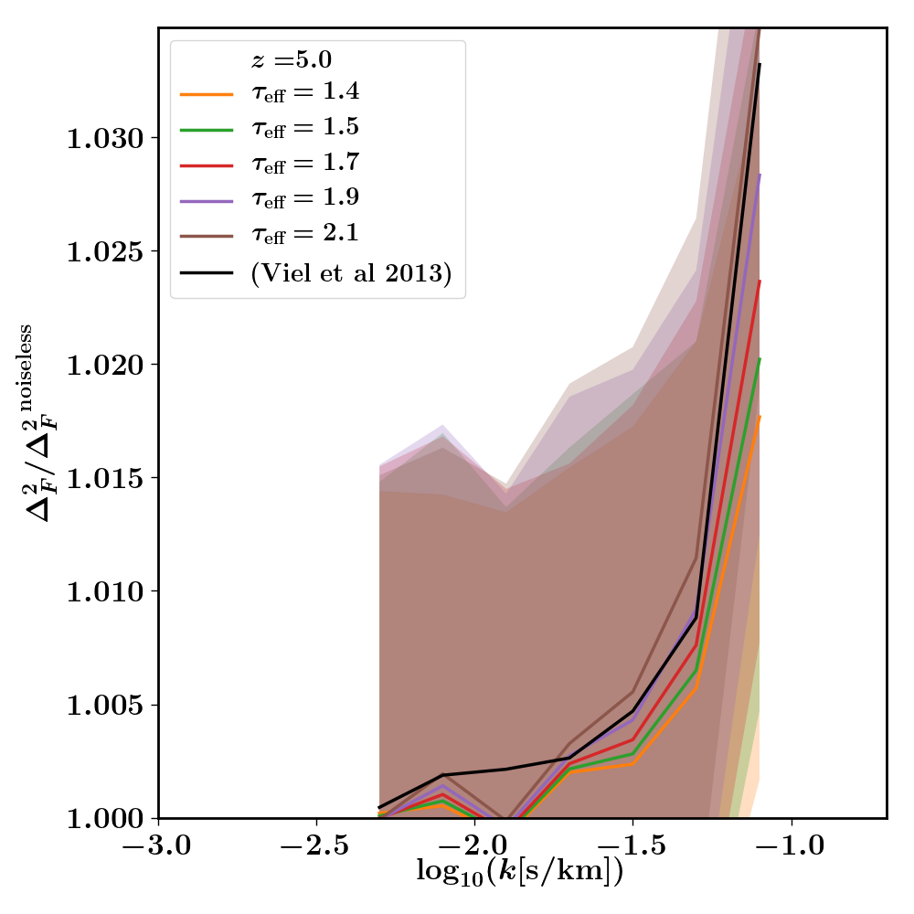
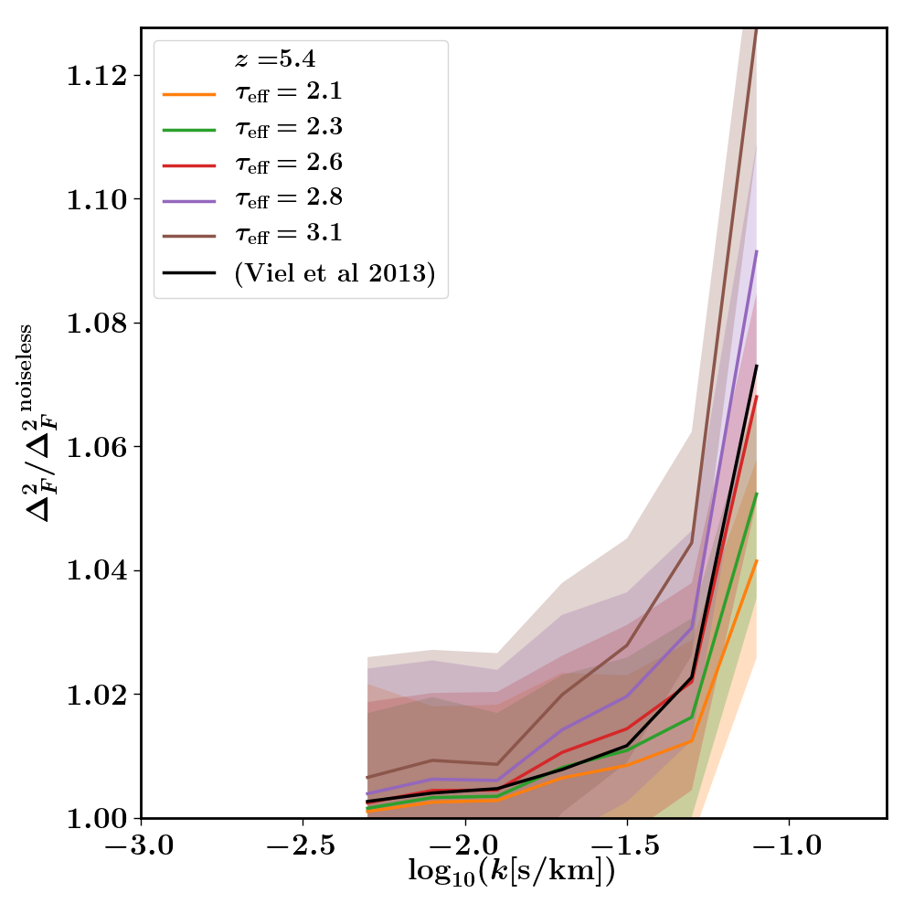
Figure 10: The effect of noise on FPS and its dependence from $\tau_{\rm eff}$. We show the ratio between the FPS computed with and without noise. We have considered a signal-to-noise ratio equal to 15, for a CDM simulation without UVB, and with imposed temperature in post-processing equal to $T=2\times 10^{4}~{}{\rm K}$. The left (right) panel regards the redshift interval centered on $z=5.0$ ($z=5.4$). The solid lines refers to the mean of the ratio between the FPS computed with and without noise, the shaded region refer to the $1$-$\sigma$ uncertainty on the ratio. The black solid line is the correction for noise applied in Viel et al. (2013a), that is independent from $\tau_{\rm eff}$. We conclude that the effect of noise depends on $\tau_{\rm eff}$, and that accounting for noise only with a filter to the noiseless FPS is going to introduce a bias in the final estimate of the temperature.

Appendix D Estimation of mean flux uncertainties

Available measurements of mean flux at high redshifts are based on small samples of quasars. Data from Viel et al. (2013a) that we are using contains only 25 quasars with emission redshifts $4.48\leq z_{\mathrm{em}}\leq 6.42$. Other works like Becker et al. (2015) provide mean flux measurements also for only $\sim 10$ redshift intervals above $z=5$. Even though quoted mean flux errors for individual spectra can be as low as $\sim 1\%$, tiny sample sizes suggest that undersampling of the density distribution is occurring.

To estimate this sampling error, we studied the distribution of mean flux for populations of mock spectra drawn from one of our simulations. To closely replicate the setup of Viel et al. (2013a), from 1000 lines of sight of the length $20\,\text{Mpc}/h$ we prepared 142 l.o.s. of $140\,\text{Mpc}/h$ by random concatenation (roughly corresponding to $\Delta z=0.4$ used in Viel et al. (2013a) to bin the observations).

Next, we drew 1000 samples of the sizes 1, 10 and 100. For each population, we computed the standard as well as maximal deviations to gauge the sampling bias: Table 4. We see that typical error for $N_{sample}=10$ is of the order of $4-5\%$.

On the other hand, the typical continuum level uncertainty is estimated to be $\sim 20\%$ (Viel et al., 2013a). Hence, uncertainty is dominated by continuum error.

Table 4: Means and standard deviations for populations of $140\,\text{Mpc}/h$ mock spectra. $\bar{F}$ denotes averaging inside a population while angular brackets $\left<\right>$ denote ensemble average.

z	$N_{\text{sample}}$	$\left<\bar{F}\right>$	Standard Deviation
5.4	1	$0.1136$	$\pm 0.0163$ $(\pm 14.3\%)$
	10	$0.1121$	$\pm 0.0056$ $(\pm 5.0\%)$
	100	$0.1121$	$\pm 0.0008$ $(\pm 0.7\%)$
5.0	1	$0.2086$	$\pm 0.0247$ $(\pm 11.8\%)$
	10	$0.2070$	$\pm 0.0078$ $(\pm 3.8\%)$
	100	$0.2065$	$\pm 0.0011$ $(\pm 0.5\%)$

Appendix E Analysis of the HIRES data-sets at $z=4.2$ and $z=4.6$

In this analysis we have considered the HIRES data-sets at $z=5.0$ and $z=5.4$ that were already presented in (Viel et al., 2013a). In that same work, the authors had analyzed there were two more HIRES data-sets at $z=4.2$ and $z=4.6$. Because we have previously shown that the previous constraints on WDM are obtained from the data at $z=5.0$ (Garzilli et al., 2017), we have focused on analyzing data at $z=5.0$ and $z=5.4$. Here, for completeness we give the results of our analysis for these later redshift intervals. In Figure 11 we show the confidence level for $\tau_{\rm eff}$ and $T_{0}$ for $z=4.2$ and $z=5.0$. In Table 5 we show the values of the $\chi^{2}$ for the best-fitting models.

Figure 11: Confidence levels of mock FPS compared to the observed FPS of hires for redshifts $z=4.2$ (left) and $z=4.6$ (right). Same convention as in Figure 6.

Table 5: Values of $\chi^{2}$ for the best-fitting models shown in Figure 11. The number of dof is 5.

model	$z$	$\chi^{2}$
CDM_Planck_Late	4.2	9.91
	4.6	4.61
M7L12_Planck_Late	4.2	6.04
	4.6	3.99

References

- Abel & Haehnelt (1999) Abel T., Haehnelt M. G., 1999, ApJ, 520, L13
- Ade et al. (2016) Ade P. A. R., et al., 2016, Astron. Astrophys., 594, A13
- Altay & Theuns (2013) Altay G., Theuns T., 2013, MNRAS, 434, 748
- Angulo et al. (2013) Angulo R. E., Hahn O., Abel T., 2013, MNRAS, 434, 3337
- Baur et al. (2016) Baur J., Palanque-Delabrouille N., Yeche C., Magneville C., Viel M., 2016, J. Cosmology Astropart. Phys, 8, 012
- Baur et al. (2017) Baur J., Palanque-Delabrouille N., Yèche C., Boyarsky A., Ruchayskiy O., Armengaud É., Lesgourgues J., 2017, J. Cosmology Astropart. Phys, 12, 013
- Becker et al. (2007) Becker G. D., Rauch M., Sargent W. L. W., 2007, Astrophys. J., 662, 72
- Becker et al. (2011) Becker G. D., Bolton J. S., Haehnelt M. G., Sargent W. L. W., 2011, MNRAS, 410, 1096
- Becker et al. (2015) Becker G. D., Bolton J. S., Madau P., Pettini M., Ryan-Weber E. V., Venemans B. P., 2015, Mon. Not. Roy. Astron. Soc., 447, 3402
- Becker et al. (2018) Becker G. D., Davies F. B., Furlanetto S. R., Malkan M. A., Boera E., Douglass C., 2018, preprint, (arXiv:1803.08932)
- Bolton et al. (2012) Bolton J. S., Becker G. D., Raskutti S., Wyithe J. S. B., Haehnelt M. G., Sargent W. L. W., 2012, MNRAS, 419, 2880
- Bosman et al. (2018) Bosman S. E. I., Fan X., Jiang L., Reed S., Matsuoka Y., Becker G., Haehnelt M., 2018, MNRAS, 479, 1055
- Boyarsky et al. (2009a) Boyarsky A., Lesgourgues J., Ruchayskiy O., Viel M., 2009a, J. Cosmology Astropart. Phys, 5, 012
- Boyarsky et al. (2009b) Boyarsky A., Lesgourgues J., Ruchayskiy O., Viel M., 2009b, Phys. Rev. Lett., 102, 201304
- Boyarsky et al. (2014) Boyarsky A., Ruchayskiy O., Iakubovskyi D., Franse J., 2014, Phys. Rev. Lett., 113, 251301
- Boyarsky et al. (2015) Boyarsky A., Franse J., Iakubovskyi D., Ruchayskiy O., 2015, Phys. Rev. Lett., 115, 161301
- Boyarsky et al. (2018) Boyarsky A., Drewes M., Lasserre T., Mertens S., Ruchayskiy O., 2018, Prog. Part. Nucl. Phys.
- Bulbul et al. (2014) Bulbul E., Markevitch M., Foster A., Smith R. K., Loewenstein M., Randall S. W., 2014, Astrophys. J., 789, 13
- Calverley et al. (2011) Calverley A. P., Becker G. D., Haehnelt M. G., Bolton J. S., 2011, Mon. Not. Roy. Astron. Soc., 412, 2543
- Croft (2004) Croft R. A. C., 2004, ApJ, 610, 642
- Davies et al. (2018) Davies F. B., et al., 2018, preprint, (arXiv:1802.06066)
- Desjacques & Nusser (2004) Desjacques V., Nusser A., 2004, MNRAS, 351, 1395
- Erkal et al. (2016) Erkal D., Belokurov V., Bovy J., Sanders J. L., 2016, MNRAS, 463, 102
- Garzilli et al. (2015) Garzilli A., Theuns T., Schaye J., 2015, MNRAS, 450, 1465
- Garzilli et al. (2017) Garzilli A., Boyarsky A., Ruchayskiy O., 2017, Phys. Lett., B773, 258
- Ghiglieri & Laine (2015) Ghiglieri J., Laine M., 2015, JHEP, 11, 171
- Gnedin & Hui (1998) Gnedin N. Y., Hui L., 1998, MNRAS, 296, 44
- Governato et al. (2010) Governato F., et al., 2010, Nature, 463, 203
- Gunn & Peterson (1965) Gunn J. E., Peterson B. A., 1965, ApJ, 142, 1633
- Haardt & Madau (1996) Haardt F., Madau P., 1996, ApJ, 461, 20
- Haardt & Madau (2001) Haardt F., Madau P., 2001, in Neumann D. M., Tran J. T. V., eds, Clusters of Galaxies and the High Redshift Universe Observed in X-rays. ArXiv astro-ph/0106018 (arXiv:astro-ph/0106018)
- Hansen et al. (2002) Hansen S. H., Lesgourgues J., Pastor S., Silk J., 2002, Mon. Not. Roy. Astron. Soc., 333, 544
- Hui & Gnedin (1997) Hui L., Gnedin N. Y., 1997, Mon. Not. Roy. Astron. Soc., 292, 27
- Hui & Haiman (2003) Hui L., Haiman Z., 2003, ApJ, 596, 9
- Hui et al. (1997) Hui L., Gnedin N. Y., Zhang Y., 1997, ApJ, 486, 599
- Iršič et al. (2017a) Iršič V., et al., 2017a, Phys. Rev. D, 96, 023522
- Iršič et al. (2017b) Iršič V., Viel M., Haehnelt M. G., Bolton J. S., Becker G. D., 2017b, Phys. Rev. Lett., 119, 031302
- Jakobsen et al. (1994) Jakobsen P., Boksenberg A., Deharveng J. M., Greenfield P., Jedrzejewski R., Paresce F., 1994, Nature, 370, 35
- Kaiser (1987) Kaiser N., 1987, Mon. Not. Roy. Astron. Soc., 227, 1
- Kaiser & Peacock (1991) Kaiser N., Peacock J. A., 1991, ApJ, 379, 482
- La Plante et al. (2017) La Plante P., Trac H., Croft R., Cen R., 2017, ApJ, 841, 87
- Laine & Shaposhnikov (2008) Laine M., Shaposhnikov M., 2008, JCAP, 0806, 031
- Lewis et al. (2000) Lewis A., Challinor A., Lasenby A., 2000, Astrophys. J., 538, 473
- Li et al. (2016) Li R., Frenk C. S., Cole S., Gao L., Bose S., Hellwing W. A., 2016, MNRAS, 460, 363
- Lidz et al. (2010) Lidz A., Faucher-Giguere C. A., Dall’Aglio A., McQuinn M., Fechner C., Zaldarriaga M., Hernquist L., Dutta S., 2010, Astrophys. J., 718, 199
- Lovell et al. (2016) Lovell M. R., et al., 2016, MNRAS, 461, 60
- Lovell et al. (2017) Lovell M. R., et al., 2017, MNRAS, 468, 4285
- Maccio et al. (2012) Maccio A. V., Paduroiu S., Schneider A., Moore B., 2012, MNRAS, 424, 1105
- Madau (2017) Madau P., 2017, ApJ, 851, 50
- McDonald et al. (2001) McDonald P., Miralda-Escude J., Rauch M., Sargent W. L. W., Barlow T. A., Cen R., 2001, Astrophys. J., 562, 52
- McDonald et al. (2005) McDonald P., Seljak U., Cen R., Bode P., Ostriker J. P., 2005, MNRAS, 360, 1471
- McGill (1990) McGill C., 1990, MNRAS, 242, 428
- McQuinn (2012) McQuinn M., 2012, MNRAS, 426, 1349
- Meiksin (2009) Meiksin A. A., 2009, Reviews of Modern Physics, 81, 1405
- Miralda-Escude & Ostriker (1990) Miralda-Escude J., Ostriker J. P., 1990, ApJ, 350, 1
- Miralda-Escude & Rees (1993) Miralda-Escude J., Rees M. J., 1993, MNRAS, 260, 617
- Miralda-Escudé & Rees (1994) Miralda-Escudé J., Rees M. J., 1994, MNRAS, 266, 343
- Mo et al. (1997) Mo H. J., Jing Y. P., Borner G., 1997, MNRAS, 286, 979
- Mortlock et al. (2011) Mortlock D. J., et al., 2011, Nature, 474, 616
- Murgia et al. (2018) Murgia R., Iršič V., Viel M., 2018, ArXiv preprint
- Navarro et al. (1996) Navarro J. F., Eke V. R., Frenk C. S., 1996, MNRAS, 283, L72
- Oñorbe et al. (2017a) Oñorbe J., Hennawi J. F., Lukić Z., 2017a, ApJ, 837, 106
- Oñorbe et al. (2017b) Oñorbe J., Hennawi J. F., Lukić Z., Walther M., 2017b, ApJ, 847, 63
- Oman et al. (2015) Oman K. A., et al., 2015, MNRAS, 452, 3650
- Pawlik et al. (2017) Pawlik A. H., Rahmati A., Schaye J., Jeon M., Dalla Vecchia C., 2017, MNRAS, 466, 960
- Planck Collaboration et al. (2016) Planck Collaboration et al., 2016, A&A, 596, A108
- Planck Collaboration et al. (2018) Planck Collaboration et al., 2018, preprint, (arXiv:1807.06209)
- Pontzen & Governato (2012) Pontzen A., Governato F., 2012, MNRAS, 421, 3464
- Pritchard & Loeb (2012) Pritchard J. R., Loeb A., 2012, Reports on Progress in Physics, 75, 086901
- Rorai et al. (2018) Rorai A., Carswell R. F., Haehnelt M. G., Becker G. D., Bolton J. S., Murphy M. T., 2018, MNRAS, 474, 2871
- Schaye (2001) Schaye J., 2001, ApJ, 559, 507
- Schaye et al. (2000) Schaye J., Theuns T., Rauch M., Efstathiou G., Sargent W. L. W., 2000, MNRAS, 318, 817
- Schaye et al. (2015) Schaye J., Crain R. A., Bower R. G., al. 2015, MNRAS, 446, 521
- Schneider et al. (2013) Schneider A., Smith R. E., Reed D., 2013, MNRAS, 433, 1573
- Scoccimarro (2004) Scoccimarro R., 2004, Phys. Rev., D70, 083007
- Scoccimarro et al. (2012) Scoccimarro R., Hui L., Manera M., Chan K. C., 2012, Phys. Rev. D, 85, 083002
- Seljak et al. (2006) Seljak U., Makarov A., McDonald P., Trac H., 2006, Phys. Rev. Lett., 97, 191303
- Shao et al. (2013) Shao S., Gao L., Theuns T., Frenk C. S., 2013, MNRAS, 430, 2346
- Shi & Fuller (1999) Shi X.-D., Fuller G. M., 1999, Phys. Rev. Lett., 82, 2832
- Springel (2005) Springel V., 2005, MNRAS, 364, 1105
- Syphers & Shull (2014) Syphers D., Shull J. M., 2014, ApJ, 784, 42
- Theuns et al. (1998) Theuns T., Leonard A., Efstathiou G., Pearce F. R., Thomas P. A., 1998, MNRAS, 301, 478
- Theuns et al. (2000) Theuns T., Schaye J., Haehnelt M. G., 2000, MNRAS, 315, 600
- Theuns et al. (2002) Theuns T., Viel M., Kay S., Schaye J., Carswell R. F., Tzanavaris P., 2002, ApJ, 578, L5
- Tremaine & Gunn (1979) Tremaine S., Gunn J. E., 1979, Physical Review Letters, 42, 407
- Upton Sanderbeck et al. (2016) Upton Sanderbeck P. R., D’Aloisio A., McQuinn M. J., 2016, MNRAS, 460, 1885
- Venumadhav et al. (2016) Venumadhav T., Cyr-Racine F.-Y., Abazajian K. N., Hirata C. M., 2016, Phys. Rev., D94, 043515
- Viel et al. (2005) Viel M., Lesgourgues J., Haehnelt M. G., Matarrese S., Riotto A., 2005, Phys. Rev., D71, 063534
- Viel et al. (2006) Viel M., Lesgourgues J., Haehnelt M. G., Matarrese S., Riotto A., 2006, Phys. Rev. Lett., 97, 071301
- Viel et al. (2013a) Viel M., Becker G. D., Bolton J. S., Haehnelt M. G., 2013a, Phys. Rev. D, 88, 043502
- Viel et al. (2013b) Viel M., Schaye J., Booth C. M., 2013b, MNRAS, 429, 1734
- Wiersma et al. (2009) Wiersma R. P. C., Schaye J., Smith B. D., 2009, MNRAS, 393, 99