Generation of magnetic skyrmions through pinning effect

Abstract

Based on analytical estimation and lattice simulation, a proposal is made that magnetic skyrmions can be generated through the pinning effect in 2D chiral magnetic materials, in absence of an external magnetic field or magnetic anisotropy. In our simulation, stable magnetic skyrmions can be generated in the pinning areas. The properties of the skyrmions are studied for various values of ferromagnetic exchange strength and the Dzyaloshinskii-Moriya interaction strength.

I Introduction

The topologically protected structure called skyrmion can be formed in a chiral magnet nagaosa ; Fert . Magnetic skyrmions have been discovered in the bulk MnSi by using neutron scattering Muhlbauer , and have also been observed by using Lorentz transmission electron microscopy Yu1 and by using spin-resolved scanning tunnelling microscopy (STM) 2DSkyrmion2 . They can be created in magnetic materials with Dzyaloshinskii-Moriya (DM) interactions DMI . They can be driven by spin current with critical current density lower than that for magnetic domain walls ultralow , and are thus promising as future information carriers in magnetic information storage and processing devices.

Therefore it is interesting to find efficient methods of creation and manipulation of magnetic skyrmions. In the presence of a magnetic field, single skyrmions can be created and deleted by using local spin-polarized STM Romming . A large number of magnetic skyrmons were created with the aid of a special geometrical constriction in presence of interfacial DM interaction bubble ; thetarho . In the absence of a magnetic field, skyrmions can be generated with the aid of a circulating current Tchoe , or magnetic anisotropy anisotropy ; bilayer1 , or perpendicular anisotropy energy anisotropyenergy , or DC current together with inhomogeneous magnetization but without DM interactions dccurrent .

Pinning effect refers to the inhomogeneities of the ferromagnetic exchange coupling, the DM interaction and the magnetic anisotropy, which may be caused by defects and impurities pin ; pin2 . In this paper, we propose a novel method to generate magnetic skyrmions by exploiting the inhomogeneities of the ferromagnetic coupling and the DMI strength.

The rest of the paper is organized as the following. In Sec. II, we briefly review the 2D magnetic skyrmions and introduce our basic idea. In Sec. III, we report a lattice simulation and study the properties of the skyrmions generated in the simulation. A summary is made in Sec. IV .

II Basic Idea

In consideration of that the skyrmions can be generated by using magnetic anisotropy, here we only consider the case without magnetic anisotropy. In this case, in the presence of an external magnetic field, the Hamiltonian can be written as nagaosa ; FreeEnergy

$$\begin{split}&{\mathcal{H}}_{\rm tot}({\bf r})=\frac{J({\bf r})}{2}\left(\nabla{\bf n}\right)^{2}+D({\bf r}){\bf n}\cdot(\nabla\times{\bf n})-{\bf B}(\bf r)\cdot{\bf n},\\ \end{split}$$ (1)

where ${\bf n}$ is the orientation of the magnetic moment, $J({\bf r})$ is the ferromagnetic exchange strength, $D({\bf r})$ is the strength of DM interaction, ${\bf B}=B\mathbf{e}_{z}$ is the external magnetic field along ${\bf e}_{z}$ direction. We use dimensionless parameters.

The local magnetic moment of a skyrmion or anti-skyrmion can be parameterized as nagaosa .

$$\begin{split}&{\bf n}(x,y)=\left(\cos(\gamma+m\phi)\sin(\theta(\rho)),\sin(\gamma+m\phi)\sin(\theta(\rho)),g\cos(\theta(\rho))\right),\\ \end{split}$$ (2)

where $\rho$ and $\phi$ are polar coordinates of the 2D position vector $(x,y)$, with the origin at the center of the skyrmion, $m=\pm 1$ is the vorticity of the skyrmion or anti-skyrmion, $g=\pm 1$ is the polarization, $\gamma$ is helicity and distinguishes between N$\rm\acute{e}$el-type and Bloch-type skyrmions, $\theta(\rho)$ is a function describing the shape of a skyrmion, with $\theta(0)=\pi$ and $\theta(\infty)=0$. The skyrmion charge is defined as nagaosa ; Tchoe

$$\begin{split}&Q=\frac{1}{4\pi}\int dxdy{\bf n}\cdot\left(\frac{\partial{\bf n}}{\partial x}\times\frac{\partial{\bf n}}{\partial y}\right)=-mg.\\ \end{split}$$ (3)

The anti-skyrmions usually result from anisotropic DM interaction antiskyrmion , but here we only consider isotropic DM interaction, hence we only consider $m=1$.

It has been found that for a skyrmion, $\theta(\rho)$ can be approximated as arctan

$$\begin{split}&\theta(\rho)\approx 4\tan^{-1}(\exp(-a\rho)).\\ \end{split}$$ (4)

Obtained from this expression with $a=0.05$, some examples of ${\bf n}({\bf r})$ are shown in Fig. 1.

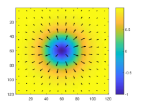
(a) $g=1$,$m=1$,$\gamma=0$

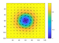
(b) $g=1$,$m=1$,$\gamma=\frac{\pi}{2}$

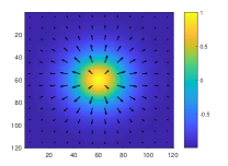
(c) $g=-1$,$m=1$,$\gamma=0$

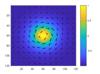
(d) $g=-1$,$m=1$,$\gamma=\frac{\pi}{2}$

Figure 1: Skyrmions characterized by ${\bf n}(\bf r)$ parameterized as in Eqs. (2) and (4), with various values of $g$ and $\gamma$. The heat map represents the magnitude of $n_{z}$ and the arrow represents $(n_{x},n_{y})$.

Two kinds of pinning were considered previously. In Ref. pin , both $J$ and $D$ are inhomogeneous, while $D/J$ is kept constant. In Ref. pin2 , $D$ is constant while $J$ is inhomogeneous. For simplicity, we only consider the latter case in this section. The former case will be studied in a lattice simulation in next section.

From Eq. (1), we obtain the Euler-Lagrange equation

$$\begin{split}&\frac{\sin(\theta)\cos(\theta)}{\rho}-\theta^{\prime}-\rho\theta^{\prime\prime}-2\frac{\tilde{D}}{J(\rho)}\sin^{2}(\theta)+\frac{\tilde{B}}{J(\rho)}\rho\sin(\theta)-\rho\frac{J^{\prime}(\rho)}{J(\rho)}\theta^{\prime}=0,\end{split}$$ (5)

where $\tilde{D}\equiv g\sin(\gamma)D$, $\tilde{B}\equiv gB$, $J(\rho)$ is a pinning function, simply assumed to depend only on $\rho$ so that the skyrmion center is at the center of the pinning, which is rotationally symmetric. When there is no pinning while an external magnetic field is applied, Eq. (5) becomes

$$\begin{split}&\frac{\sin(\theta)\cos(\theta)}{\rho}-\theta^{\prime}-\rho\theta^{\prime\prime}-2\frac{\tilde{D}}{J}\sin^{2}(\theta)+\frac{\tilde{B}}{J}\rho\sin(\theta)=0.\\ \end{split}$$ (6)

It is known that the skyrmions can be generated in this case.

We note that when pinning is present, $J^{\prime}$ term in Eq. (5) plays a role similar to that of $\tilde{B}$ term. Using the ansatz $\theta(\rho)$ in Eq. (4) for $b\sin(\theta(\rho))=J^{\prime}(\rho)\theta^{\prime}(\rho)$, where $b$ is some value of $\tilde{B}$ , we find that if

$$\begin{split}&J(\rho)=J_{0}+b\frac{a\rho+\log\left(e^{-2a\rho}+1\right)}{a^{2}},\end{split}$$ (7)

where $a$ as given in Eq. (4), $J_{0}$ is an undetermined coefficient, then Eq. (5) without $\tilde{B}$ term becomes

$$\begin{split}&\frac{\sin(\theta)\cos(\theta)}{\rho}-\theta^{\prime}-\rho\theta^{\prime\prime}-2\frac{\tilde{D}}{J(\rho)}\sin^{2}(\theta)+\frac{b}{J(\rho)}\rho\sin(\theta)=0,\\ \end{split}$$ (8)

which is very close to Eq. (6) except that the $J$ is now position dependent.

With $J(\rho)$ in Eq. (7) as an ansatz, we solve Eq. (5) in the absence of $\tilde{B}$ term, using the numerical method in Ref. pin , which proposed a mechanism of pinning skyrmions. We choose the parameter values to be $J_{0}=1$, $\tilde{B}=0$, $\tilde{D}=0.05$, $b=0.005$, $a=0.05$. As shown in Fig. 2, the solution is very close to the skyrmion ansatz (4), suggesting that it is possible to create skyrmions by using the pinning effect.

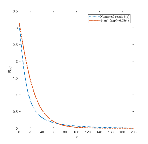
Figure 2: The dotted line represents the numerical result of Euler-Lagrange Equation (5) with $\tilde{B}=0$. The dotted-dashed line represents the skyrmion ansatz (4).

III Lattice simulation

The above estimation with an artificial pinning effect suggests the possibility of really creating a skyrmion using pinning effect only. Since the effective parameter $\tilde{D}$ depends not only on $D$ but also on the parameters of the skyrmions, whether or not a solution of $\theta(\rho)$ can be identified as a skyrmion is technically subtle. Therefore, rather than solving the Euler-Lagrange equation, we perform a lattice simulation, which directly provides evidence of skyrmions.

We now consider more realistic pinning effect. As a local structure, the effect of pinning should be suppressed very quickly in deviating away from the pinning center. An exponentially decaying function $J(\rho)$ is assumed in Ref. pin2 , while a Gaussian function $J(\rho)$ is assumed in Ref. pin . We follow Ref. pin to assume $J(\rho)$ to be Gaussian,

$$\begin{split}&J(\rho)=J_{0}+J_{1}e^{-J_{2}\rho^{2}},\end{split}$$ (9)

where $J_{0}$, $J_{1}$ and $J_{2}$ are undetermined coefficients, with $J_{0}>0$, $J_{1}>-J_{0}$ and $J_{2}>0$. The radius of the pinning is denoted as $R_{p}$, and $R_{p}\sim 1/\sqrt{J_{2}}$.

In the simulation, as dimensionless parameters, $J=1$ is used as the definition of the energy unit, $J(\infty)=J_{0}=1$ is assumed for simplicity unitJ ; alpha3 ; bilayer . The dimensionless quantities can be rescaled to physical ones as the following Tchoe ; unitJ ; pin . The time unit $\Delta t=1$ in the simulation represents $t=\hbar/J$ in physical time. The rescaling factor $r$ can be determined from the helical wavelength $\lambda$ and the lattice spacing $a$, as $r=(D/J)\lambda/(2\pi\sqrt{2}a)$. Then the time is rescaled as $t^{\prime}=r^{2}t$. For example, if we adopt the real material such that $\lambda\approx 60\;{\rm nm}$ and $a\approx 4\;{\AA}$ and with $D/J=0.5$, we find $r\approx 8.44$. Then, if we adopt the energy unit as $J=3\;{\rm meV}$, then $t^{\prime}=r^{2}\hbar/J\approx 220r^{2}\;{\rm fs}\approx 0.016\;{\rm ns}$.

The lattice simulation is based on the Landau-Lifshitz-Gilbert (LLG) equation nagaosa ; pin ; LLG ; LLG2

$$\begin{split}&\frac{d}{dt}{\bf n}_{\bf r}=-{\bf B}_{\rm eff}({\bf r})\times{\bf n}_{\bf r}-\alpha{\bf n}_{\bf r}\times\frac{d}{dt}{\bf n}_{\bf r},\\ \end{split}$$ (10)

where ${\bf n}_{\bf r}$ is the local magnetic moment at site ${\bf r}$, $\alpha$ is the Gilbert damping constant, ${\bf B}_{\rm eff}$ is the effective magnetic field,

$$\begin{split}&{\bf B}_{\rm eff}({\bf r})=-\frac{\delta H}{\delta{\bf n}_{\bf r}},\end{split}$$ (11)

with the discrete Hamiltonian unitJ ; discreteH

$$\begin{split}&H=\sum_{{\bf r},i=x,y}\left[-J({\bf r}){\bf n}_{{\bf r}+\delta_{i}}-D({\bf r}){\bf n}_{{\bf r}+\delta_{i}}\times{{\bf e}}_{i}-{\bf B}\right]\cdot{\bf n}_{\bf r},\\ \end{split}$$ (12)

where $\delta_{i}$ refers to each neighbour, and $\delta_{i}={\bf e}_{i}$ on a square lattice. So pin

$$\begin{split}&{\bf B}_{\rm eff}({\bf r})=\sum_{i=x,y}\left[J({\bf r}){\bf n}_{{\bf r}+\delta_{i}}+J({\bf r}-\delta_{i}){\bf n}_{{\bf r}-\delta_{i}}\right]\\ &+\sum_{i=x,y}\left[D({\bf r}){\bf n}_{{\bf r}+\delta_{i}}\times{{\bf e}}_{i}-D({\bf r}-\delta_{i}){\bf n}_{{\bf r}-\delta_{i}}\times{{\bf e}}_{i}\right]+{\bf B}({\bf r}).\end{split}$$ (13)

Unless specified otherwise, the simulation is run on a $512\times 512$ square lattice with open boundary condition and ${\bf B}=0$, and with the pinning center set to be at the point $(256,256)$. In the following, we denote the time step as $\Delta t$, and the time in unit of $\Delta t$ the simulation takes is denoted as $\tau$. The number of step is $\tau/\Delta t$. The simulation is run on the GPU, which has a great advantage over CPU on this problem. Because ${\bf n}_{{\bf r}}$’s for different sites at a same instant are independent of each other, we use GPU to do parallel computing. Within the simulation, the LLG is numerically integrated by using fourth-order Runge-Kutta method.

III.1 Skyrmion generation from random initial configurations

We first run the simulation for $J_{1}=3$, $J_{2}=0.001$ and various values of $D$. The simulation starts from randomized ${\bf n}_{\bf r}$’s and stops when ${\bf n}_{\bf r}$’s become stable. Previously, the Gilbert constant is taken to be $\alpha=0.01$ to $1$ pin ; LLG2 ; antiskyrmion ; arctan ; alpha1 ; alpha2 ; alpha3 ; bilayer . We find that the larger the value of $\alpha$, the more rapid the simulation is completed, while the smaller the value of $D$, the longer the simulation time. Hence we use $\alpha=0.1$ LLG2 ; alpha2 and $\Delta t=0.002$ for $D\geq 0.1$, while $\alpha=0.2$ pin ; alpha3 and $\Delta t=0.01$ for $D<0.1$.

The results are shown in Fig. 3. We run the simulation for $D=1,0.8,0.5,0.2,0.1,0.08,0.05,0.03,0.02,0.01$. For each value of $D$ except the smallest ones $D=0.02$ or $0.01$, a skyrmion can be generated at the pinning center. When $D$ is smaller, it takes longer time to generate the skyrmion. Generally speaking, the time needed to generate a skyrmion by using pinning is longer than generation of a skyrmion by using an external magnetic field.

(a) $D=1$,$\tau=60000\Delta t=120$,$g=1$,$m=1$,$\gamma\approx 1.58$,$R_{s}\approx 10.5$

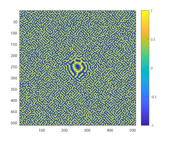
(b) $D=0.8$,$\tau=1000$,$g=1$,$m=1$,$\gamma\approx 1.56$,$R_{s}\approx 15.4$

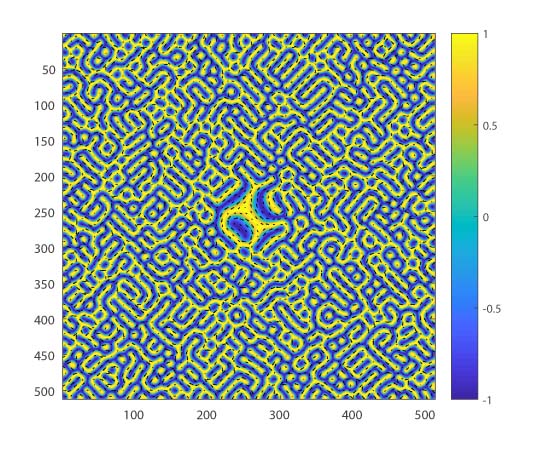
(c) $D=0.5$,$\tau=10000$,$g=1$,$m=1$,$\gamma\approx 1.57$,$R_{s}\approx 20.3$

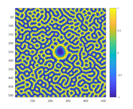
(d) $D=0.3$,$\tau=3000$,$g=1$,$m=1$,$\gamma\approx 1.57$,$R_{s}\approx 34.4$

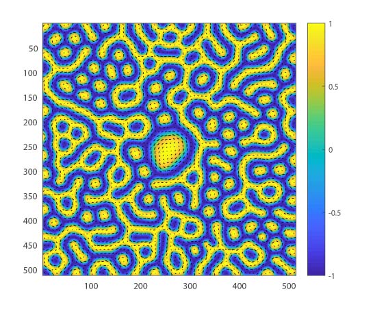
(e) $D=0.2$,$\tau=10000$,$g=-1$,$m=1$,$\gamma\approx 4.72$,$R_{s}\approx 42.6$

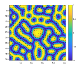
(f) $D=0.1$,$\tau=16000$,$g=-1$,$m=1$,$\gamma\approx 4.71$,$R_{s}\approx 59.8$

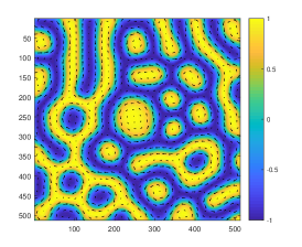
(g) $D=0.08$,$\tau=30000$,$g=-1$,$m=1$,$\gamma\approx 4.71$,$R_{s}\approx 64.8$

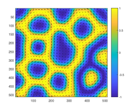
(h) $D=0.05$,$\tau=100000$,$g=1$,$m=1$,$\gamma\approx 1.57$,$R_{s}\approx 96.7$

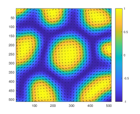
(i) $D=0.03$,$\tau=100000$,$g=-1$,$m=1$,$\gamma\approx 4.71$,$R_{s}\approx 128.3$

Figure 3: The stable spin configuration ${\bf n}_{r}$ in the lattice simulation, for $J_{1}=3$ and various values of other parameters. We find that the skyrmions can be generated at the pinning centers, by using the pinning effect only.

We have also studied the properties of the skyrmions generated in the simulation. Only those skyrmions near the pinning centers are considered. For each skyrmion considered, $g$ is determined from $n_{z}$ at the center. The radius $R_{s}$ of each skyrmion can be determined from the iso-height contour with $n_{z}=\mp 1$ for $g=\pm 1$ respectively, because $n_{z}$ varies from $\pm 1$ at the center to $\mp 1$ on the edge. In the actual simulation, however, $n_{z}$ can only approach $\mp 1$. Hence, $R_{s}$ is estimated from the radius of the iso-height contour with $n_{z}=\mp 0.9$ for $g=\pm 1$, respectively. $\gamma$ is determined by using $n_{x}$ and $n_{y}$ at the iso-height contour with $n_{z}=0$.

We first investigate the relation between the skyrmion radius $R_{s}$ and the DM interaction strength $D$. We find that the larger the value of $D$, the smaller $R_{s}$. As shown in Fig. 4, the relation between $R_{s}$ and $D$ is about

$$a+b\frac{1}{\sqrt{D}},$$ (14)

which explains why skyrmions are not generated for $D=0.02$ or $D=0.01$, as for small values of $D$, the radius of the skyrmion is too large for the lattice size.

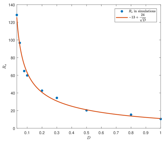
Figure 4: The relation between skyrmion radius $R_{s}$ and the DM interaction strength $D$.

All the skyrmions appearing in the simulation are of $m=1$. Then the skyrmion number $Q=-mg$ is determined from the sign of $g$. As shown in Fig. 3, skyrmions with $g=1$ and $g=-1$ can both be generated. For a skyrmion generated in an external magnetic field, $g$ is determined by the direction of ${\bf B}$. But for a skyrmion generated by using the pinning effect in absence of a magnetic field, the sign of $g$ becomes a free choice and depends on the initial state. This is verified in simulations starting with different randomized initial states but with the same values of various parameters. For $D>0$, we find that $\gamma\approx\pi/2$ for $g=1$, while $\gamma\approx-\pi/2$ for $g=-1$, hence $\tilde{D}>0$ in both cases. This can be understood by considering

$$\begin{split}&H_{\rm DM}=D{\bf n}\cdot\left(\nabla\times{\bf n}\right)=gD\sin\left((m-1)\phi+\gamma\right)\left(\frac{m}{2\rho}\sin(2\theta(\rho))+\theta^{\prime}(\rho)\right),\\ \end{split}$$ (15)

which differs from the special case of $g=1$ nagaosa in replacing $D$ as $gD$. As a result, the sign of $g$ is a free choice, while the sign of $\gamma$ is determined by $gD$. Hence the energy is lowest when $\tilde{D}>0$ and $\gamma=\pm\pi/2$ with the sign of $\gamma$ determined by $gD$, that is, $\gamma=\pi/2$ when $gD>0$, while $\gamma=-\pi/2$ when $gD<0$.

We have also studied the case of $J_{1}<0$. Using $J_{1}=-0.5$, $J_{2}=0.0001$, $\alpha=0.2$, and $\Delta t=0.01$, skyrmions are generated in the simulation (Fig. 5). In this case, the range of the value of $D$ in which skyrmions can be generated is narrower than the case of $J_{1}=3$ and $J_{2}=0.001$. Similar to the case of $J_{1}>0$, the radius of the skyrmion also increases with the decrease of $D$, and $\tilde{D}>0$ for all the skyrmions generated.

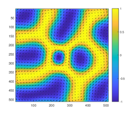
(a) $D=0.03$,$\tau=100000$,$g=1$,$m=1$,$\gamma\approx 1.5727$,$R_{s}\approx 48.6$

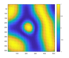
(b) $D=0.02$,$\tau=120000$,$g=-1$,$m=1$,$\gamma\approx 4.7060$,$R_{s}\approx 84.6$

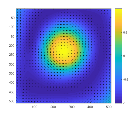
(c) $D=0.01$,$\tau=140000$,$g=-1$,$m=1$,$\gamma\approx 4.7165$,$R_{s}\approx 182.0$

Figure 5: The stable spin configuration ${\bf n}_{r}$ in the lattice simulation for $D=0.03,0.02,0.01$. The heat map represents the magnitude of $n_{z}$, the arrow represents $(n_{x},n_{y})$. In (a), only the skyrmion at the center is considered.

III.2 Skyrmion generation from helical phase

We have also studied a more realistic situation. Starting with the helical phase, we suddenly switch on the pinning, by substituting the constant $J$ with an inhomogeneous $J(\rho)$. In previous works, $D/J\approx 0.09\sim 0.5$ Tchoe ; pin ; unitJ ; alpha3 ; bilayer ; LLG2 ; discreteH ; dvalue , therefore we use $D/J_{0}=0.08,0.1,0.2,0.3,0.5$. In absence of an external magnetic field and with constant $J$, the initial state is prepared by relaxing from a saturated state with ${\bf n}_{\bf r}={\bf e}_{z}$ until the stability is reached. Thus the helical phase is obtained. Then we substitute the constant $J$ with inhomogeneous $J(\rho)$ at $\tau=0$ and continue the simulation. For $D=0.08$, we use $\alpha=0.2$ and $\Delta t=0.01$. For $D=0.1,0.2,0.3,0.5$, we use $\alpha=0.1$ and $\Delta t=0.002$.

The results for $D=0.5$, $J_{1}=3$ and $J_{2}=0.0001$ are shown in Fig. 6. The strip width increases with the decrease of $D/J$. So the stripes are wider near the pinning center, where $D/J$ is smaller. The stripes start to grow at $\tau=0$. Then a kind of turbulence is created, and small skyrmions are generated, some of which finally become stable.

The cases for $D=0.08,0.1,0.2,0.3$ are shown in Fig. 7. For $D=0.2,0.3$, we still use $J_{2}=0.0001$, as in the case of $D=0.5$. The size of the pinning should be much larger than the width of the stripes. Hence for smaller values of $D$, $J_{2}$ is chosen to be smaller, consequently the lattice is set to be larger. Therefore, for $D=0.08,0.1$, we run the simulation on a $1024\times 1024$ lattice. We choose $J_{2}=0.000025$ and set the pinning center to be at $(512,512)$. For all these cases, skyrmions are generated in the pinning region (Fig. 7), although they are not at the pinning center, as in the cases starting with randomized initial state.

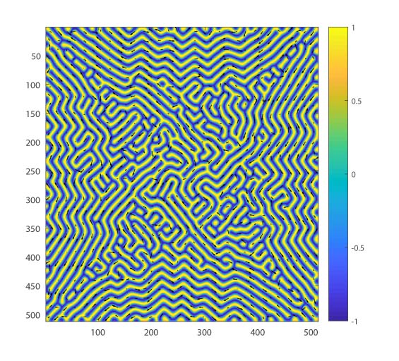
(a) $\tau=0$

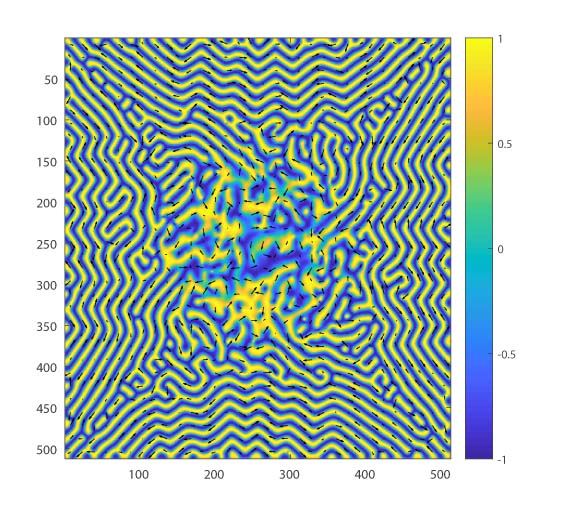
(b) $\tau=40$

(c) $\tau=80$

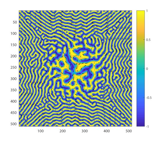
(d) $\tau=160$

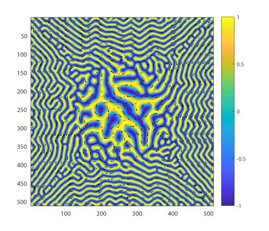
(e) $\tau=400$

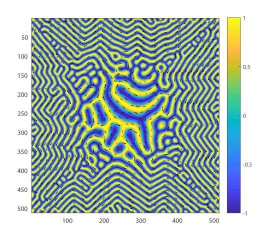
(f) $\tau=10000$

Figure 6: Simulation starting from helical phases with $D=0.5$. Pinning is switched on by suddenly substituting the constant $J$ with $J(\rho)$, with $J_{1}=3,J_{2}=0.0001$. With inhomogeneous $J(\rho)$, the stripes grow while turbulence is created and small skyrmions are generated, some of which become stable finally.

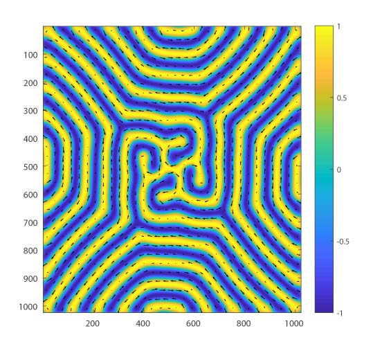
(a) $D=0.08,\tau=0$

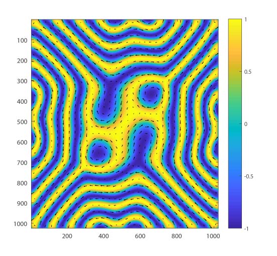
(b) $D=0.08,\tau=50000$

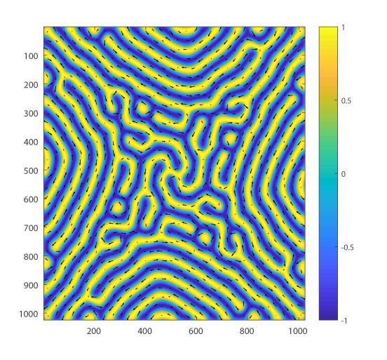
(c) $D=0.1,\tau=0$

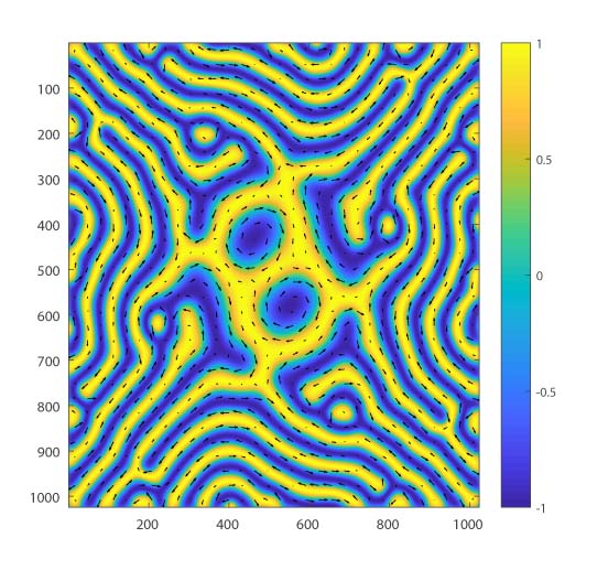
(d) $D=0.1,\tau=12000$

(e) $D=0.2,\tau=0$

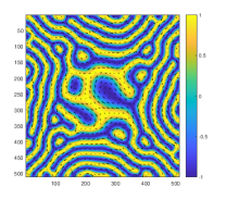
(f) $D=0.2,\tau=10000$

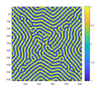
(g) $D=0.3,\tau=0$

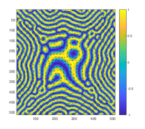
(h) $D=0.3,\tau=10000$

Figure 7: Simulation starting from helical phases. Pinning is applied by suddenly substituting the constant $J$ with $J(\rho)$. For $D=0.2,0.3$, $J_{1}=3,J_{2}=0.0001$. For $D=0.08,0.1$, we run the simulation on a $1024\times 1024$ lattice, with $J_{1}=3,J_{2}=0.000025$ and the pinning center locating at $(512,512)$. In each figure, skyrmions are generated in the pinning region, though not at the pinning center. Some skyrmions originate from short stripes close to skyrmions, but new skyrmions are also generated.

For $D=0.3$, we run the simulation on a $1024\times 1024$ lattice, with $5$ pinning centers locating at sites ${\bf r}_{1}=(512,512)$, ${\bf r}_{2}=(256,512)$, ${\bf r}_{3}=(768,512)$, ${\bf r}_{4}=(512,256)$ and ${\bf r}_{5}=(512,768)$, respectively,

$$\begin{split}&J({\bf r})=1+3\sum_{i=1}^{5}\exp\left(-0.00025({\bf r}-{\bf r}_{i})^{2}\right),\end{split}$$ (16)

with $J_{2}=0.00025$. The result (Fig. 8) shows that skyrmions are generated near some but not all of the pinning centers.

(a) $\tau=0$

(b) $\tau=3000$

Figure 8: Simulation starting from a helical phase, with $D=0.3$. There are $5$ pinning centers at the sites $(512,512)$, $(256,512)$, $(768,512)$, $(512,256)$ and $(512,768)$, all with $J_{2}=0.00025$. The pinning radii are smaller than the those in Fig. 7. (c) and (d). The skyrmions are generated in the pinning regions near $(256,512)$, $(768,512)$, $(512,256)$ and $(512,768)$, but not near $(512,512)$, where the spin structure is not topologically separated from the other stripes.

We also find that, for $J_{1}<0$, skyrmions cannot be generated by using this method.

III.3 Skyrmion generation with both $J$ and $D$ inhomogeneous

Although the origins of the ferromagnetic exchange and DM interaction are different, it is difficult to vary $J$ while keeping $D$ constant in real experiments. We also simulate a scenario in which both $J$ and $D$ inhomogeneous while $D/J$ constant, that is, $D$ has the same $\rho$-dependence as $J$ pin . When $D/J$ is homogeneous, the widths of the stripes are not changed. In this case, skyrmions cannot be generated from helical phases. However, skyrmions can still be generated at the pinning center through the pinning effect with the aid of the boundary condition, in the following way.

In our simulation, when an external magnetic field is applied, ${\bf n}_{\bf r}$ can be saturated to ${\bf n}_{\rm r}={\bf e}_{z}$ no matter whether pinning is presented. If we suddenly switch off the external magnetic field and start the simulation from a saturated initial configuration, the boundary condition plays an important role. Because of DM interaction, ${\bf n}_{\bf r}$ tends to tilt to its neighbours. If $D$ is homogenous, the tilt starts from the sites on the boundary (Fig. 9). When $D$ is inhomogeneous, the tilt starts from both the boundary and the sites with inhomogeneous $D$. This can be understood by using LLG in Eq. (11), which can be rewritten as

$$\begin{split}&\frac{d{\bf n}}{dt}=\frac{1}{1+\alpha^{2}}\left({\bf N}+\alpha{\bf N}\times{\bf n}\right),\end{split}$$ (17)

with ${\bf N}={\bf B}_{\rm eff}\times{\bf n}$. When ${\bf n}_{\bf r}={\bf e}_{z}$ and $D$ is homogeneous, ${\bf B}_{\rm eff}\propto{\bf n}_{\bf r}$ and ${\bf N}=0$. However, when $D$ is inhomogeneous, ${\bf N}\neq 0$, therefore ${\bf n}_{\bf r}$ of the sites at the boundary or at the sites with inhomogeneous $D$ start to tilt first.

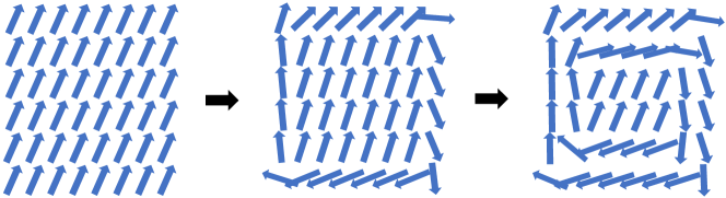
Figure 9: When the simulation starts from ${\bf n}_{\bf r}={\bf e}_{z}$, the boundary plays an important role. With DM interaction, ${\bf n}_{\bf r}$ at a site tends to tilt to its neighbours. If $D$ is homogenous, the tilt starts from the boundary.

For $D/J=0.08$, we use $J_{1}=3$, $J_{2}=0.001$, $\alpha=0.2$, $\Delta t=0.002$. The result is shown in Fig. 10. Because of the inhomogeneous $D$, a ring domain wall is generated around the pinning and keeps shrinking to the center of the ring. The center of the ring is a skyrmion. The ring keeps shrinking until about $\tau=200$, then the skyrmion at the center starts to grow until it is constrained by the domain walls generated from the boundary.

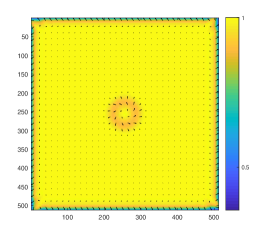
(a) $\tau=20$

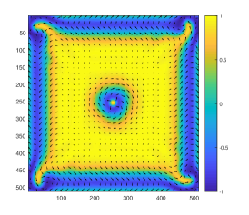
(b) $\tau=200$

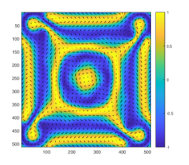
(c) $\tau=400$

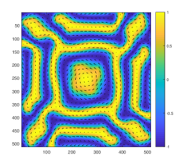
(d) $\tau=600$

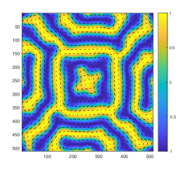
(e) $\tau=800$

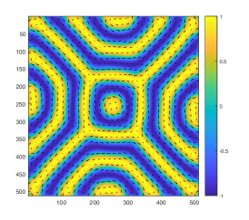
(f) $\tau=5000$

Figure 10: Simulation for $D/J=0.08$, $J_{1}=3$, $J_{2}=0.001$. Because of the inhomogeneous $D$, a ring domain wall is generated around the pinning at about $\tau=20$ and keeps shrinking to the center of the ring. The center of the ring is a skyrmion. The ring keeps shrinking until about $\tau=200$, then the skyrmion at the center starts to grow until it is constrained by the domain walls generated from the boundary.

For $D/J=0.1$, $0.2$, $0.3$, $0.5$, with the same values of other parameters as for $D/J=0.08$, stable skyrmions cannot be generated, because the skyrmion generated at the center keeps expanding and becomes very large before it meets the domain walls generated from the boundary, so its border splits into stripes. However, if we use $J_{1}<0$, domain walls are generated as several rings around the pinning and expand, as shown in Fig. 11 for $D/J=0.3$. Then if the pinning radius is close to the stripe widths, the skyrmions can be generated at the pinning center inside the smallest ring.

We run the simulation for $D/J=0.1,0.2,0.3,0.5$ with $\alpha=0.1,\Delta t=0.002$ and $J_{2}=0.00156,0.00625,0.012,0.045\sim 1/D^{2}$. For $J_{1}<0$, $J_{1}$ is related to the gap between the rings. For $D/J=0.1,0.2,0.3$, we use $J_{1}=-0.5$. For $D/J=0.5$, the gap is too large compared with the stripe widths, so we use $J_{1}=-0.85$ to make gap narrower. The result for $D/J=0.3$ is shown in Fig. 11 and the results for $D/J=0.1,0.2,0.5$ are shown in Fig. 12.

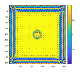
(a) $\tau=200$

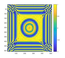
(b) $\tau=400$

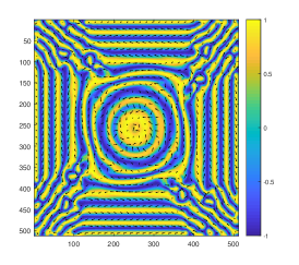
(c) $\tau=600$

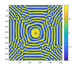
(d) $\tau=800$

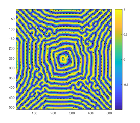
(e) $\tau=1000$

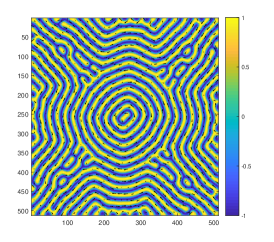
(f) $\tau=10000$

Figure 11: Simulation for $D/J=0.3,J_{1}=-0.5,J_{2}=0.012$. Because of the inhomogeneous $D$, a few domain walls are generated as rings around the pinning and keep expanding. The center of the smallest ring is a skyrmion. The largest ring keeps expanding until it meets the domain walls generated from the boundary. The smaller rings keep expanding until they are constrained by the larger rings. Finally, the center of the smallest ring becomes a skyrmion.

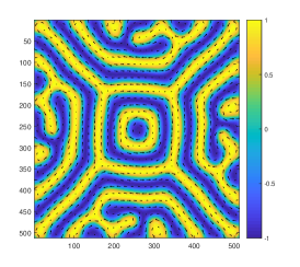
(a) $D/J=0.1,J_{1}=-0.5,J_{2}=0.00156,\tau=16000$

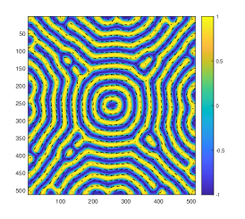
(b) $D/J=0.2,J_{1}=-0.5,J_{2}=0.00625,\tau=8000$

(c) $D/J=0.5,J_{1}=-0.85,J_{2}=0.045,\tau=10000$

Figure 12: Simulation for $J_{1}<0$. For the case $D/J=0.5$, there is a short stripe cut off from all the others. It is the center of the smallest ring similar to Fig.11, which can be considered as a stretched skyrmion.

Comparing the final states in Sec.III.3 with the initial states in Sec.III.2, we can conclude that, with boundary condition alone, the skyrmions are not generated at the center. Therefore, the effect of the pinning is essential. We also run a simulation to testify how important the boundary condition is. In real experiments, the material could be much larger, and the pinning could be located away from the center of the material. We run a simulation on a $2048\times 2048$ lattice with the pinning located at $(1200,700)$ to investigate the generation of the skyrmion in this situation. We choose $D/J=0.2$, and follow the rescaling method in Refs. Tchoe ; pin . If for the real material, $\lambda\approx 60\;{\rm nm}$, $a\approx 4\;{\AA}$, the rescaling factor is $r\approx 3.38$, therefore, a $2048\times 2048$ lattice corresponds to about $2.77\;{\rm\mu m}\times 2.77\;{\rm\mu m}$. For $J=3\;{\rm meV}$, the dimensionless time $\tau=15000$ corresponds to $37.6\;{\rm ns}$. We run the simulation with $\alpha=0.2$, $\Delta t=0.01$, $J_{1}=-0.8$ and $J_{2}=0.005$. The result is shown in Fig.13. We find that, a skyrmion is generated on the left of the pinning center, and the distance between the skyrmion center and the pinning center is about $50$, corresponding to $67.5\;{\rm nm}$ if we use the above realistic parameter values.

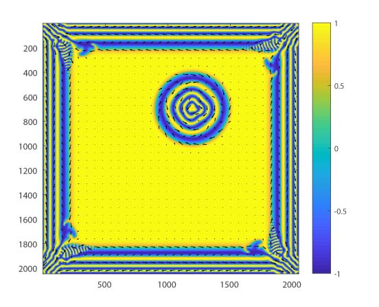
(a) $\tau=2000$

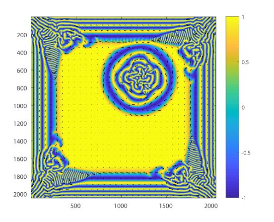
(b) $\tau=3000$

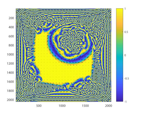
(c) $\tau=4000$

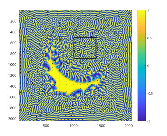
(d) $\tau=5000$

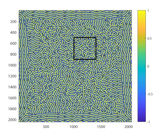
(e) $\tau=15000$

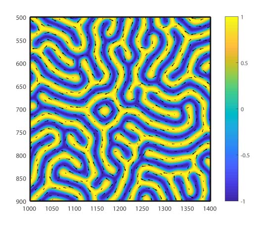
(f) $\tau=15000$

Figure 13: Simulation on a $2048\times 2048$ lattice with $D/J=0.2,\alpha=0.2$, $\Delta t=0.01$, $J_{1}=-0.8$, $J_{2}=0.005$, and the center of the pinning placed at $(1200,700)$. First, the rings appear and expand. At about $\tau=3000$, the rings meet the domain walls generated from the boundary. The center of the rings becomes stable at about $\tau=5000$. Finally, the central region of the smallest ring survives as a skyrmion, however, its position deviates from the the pinning center.

III.4 Bound states

In the simulation starting from randomized initial state, we also observe an interesting phenomenon when $D$ is constant and very small while $J_{1}<0$ (Figs. 14 and  15). It does not show up when $J_{1}>0$ or $J_{1}=0$ (no pinning), so it is a special case in presence of pinning with $J_{1}<0$. When $D$ is very small, a skyrmion and an anti-skyrmion with $g=\pm 1$ and $m=\pm 1$ are generated and move to the pinning center. They keep rotating around each other with the distance shrinking till annihilation. Previously, it was found that the interaction between two skyrmions on two layers with opposite skyrmion charge can form a bound state bilayer .

On a single layer, in contrast, if the skyrmions are generated in an external magnetic field, the sign of $g$ is determined by the external magnetic field, and whether a skyrmions or an anti-skyrmions is generated depends on $D$, then the bound states of skyrmions and anti-skyrmions are usually difficult to realize. The situation we consider may provide a novel avenue to study such bound states in a single layer.

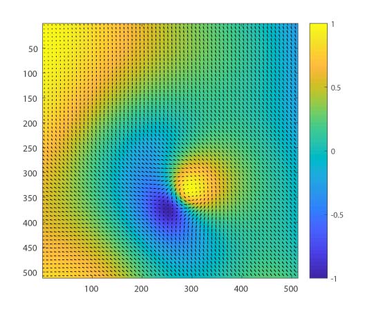
(a) $\tau=100000$

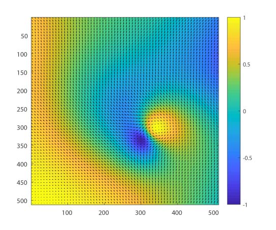
(b) $\tau=120000$

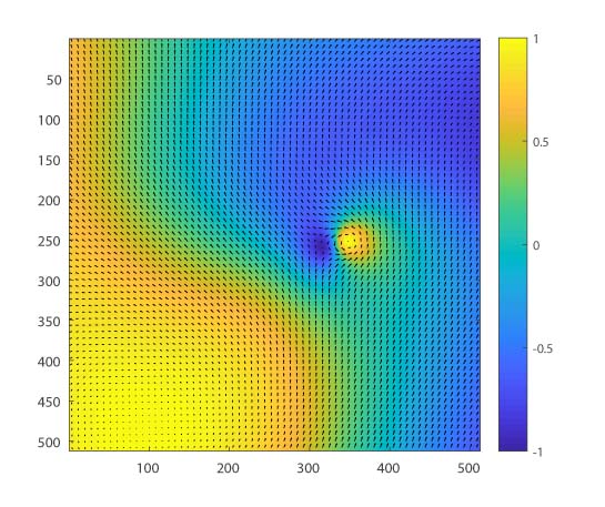
(c) $\tau=140000$

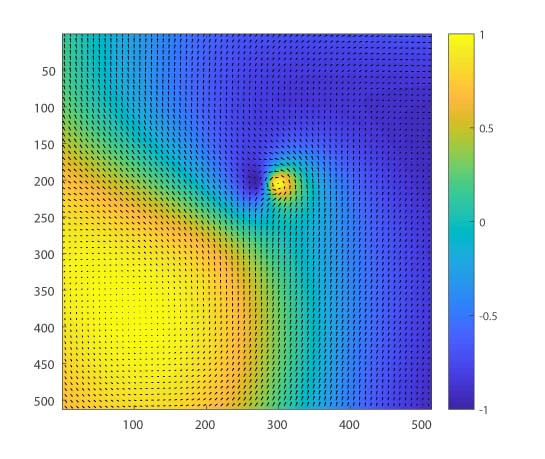
(d) $\tau=160000$

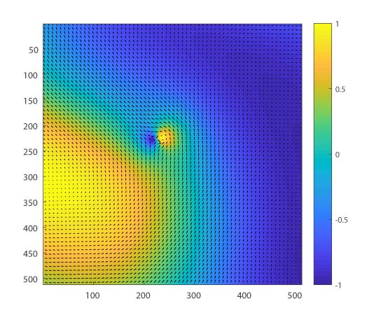
(e) $\tau=180000$

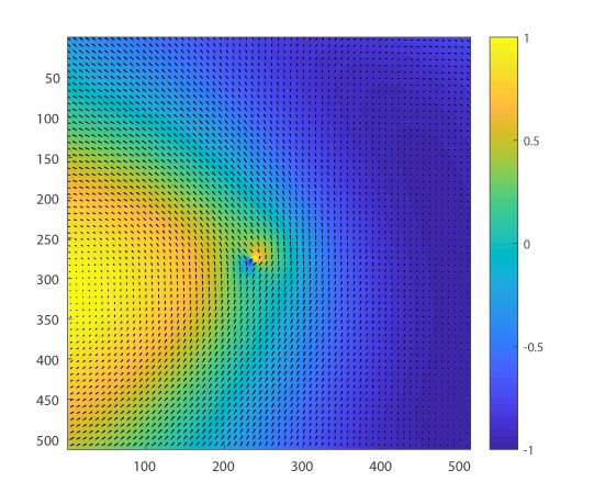
(f) $\tau=200000$

Figure 14: Simulation of skyrmion generation, with parameter values $J_{1}=-0.5$, $J_{2}=0.0001$, $D=0.005$, $\alpha=0.2$ and $\Delta t=0.01$. A skyrmion and an anti-skyrmion with $g=\pm 1$ and $m=\pm 1$ respectively rotate around each other and move to the pinning center, with the distance shrinking till annihilation.

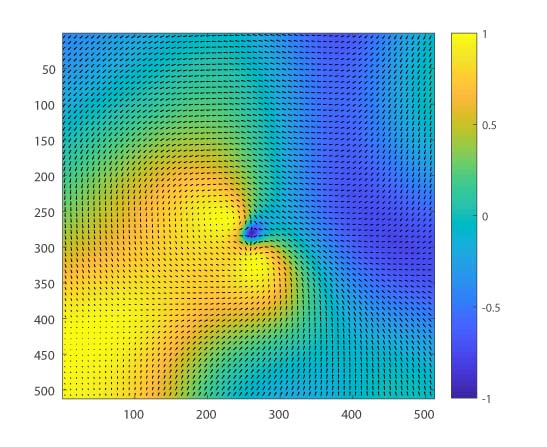
(a) $\tau=100000$

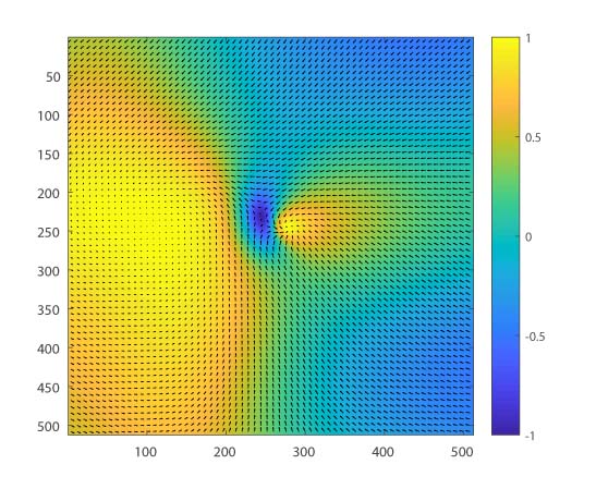
(b) $\tau=120000$

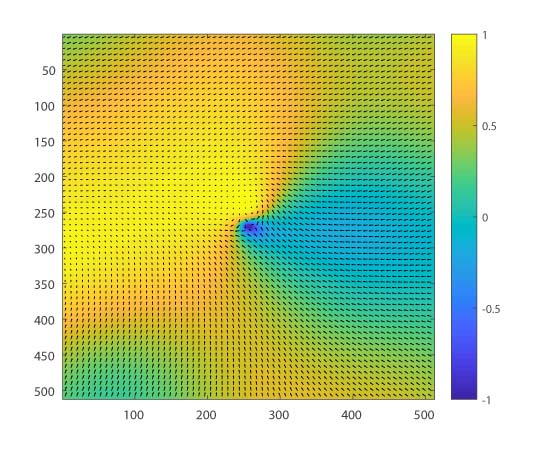
(c) $\tau=140000$

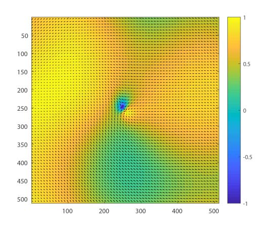
(d) $\tau=160000$

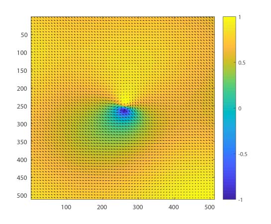
(e) $\tau=180000$

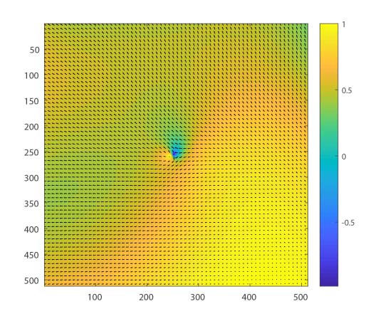
(f) $\tau=200000$

Figure 15: Simulation of skyrmion generation, with parameter values $J_{1}=-0.9$, $J_{2}=0.0001$, $D=0.003$, $\alpha=0.1$ and $\Delta t=0.01$. A skyrmion and an anti-skyrmion, with $g=\pm 1$ and $m=\pm 1$ respectively, are generated at the pinning center. Each skyrmion self-rotates. The simulation stopped at $\tau=200000$, however. As the distance shrinks, the pair is expected to annihilate.

IV Summary

In this paper, we propose a novel mechanism to generate magnetic skyrmions without the need of an external magnetic field or magnetic anisotropy. We find that skyrmions can be generated through the pinning effect only, i.e., with magnetic exchange strength $J$ inhomogeneous, or with $J$ and DM interaction $D$ both inhomogeneous. Our lattice simulation has verified this idea. In the simulation, we study the properties of the skyrmions generated under various parameter values. We find that the radius of the skyrmion increases when $D$ decrease. We also find that all the skyrmions generated have $m=1$ and $\tilde{D}>0$, while the sign of $g$ depends on the initial state. For $J_{1}<0$, we also find the generation of a pair of skyrmions with opposite $g$ and $m$ at the pinning centers.

That the skyrmions can be generated by using the pinning effect only is useful for practical applications of the magnetic skyrmions. Through the engineering of pinning in the designated site, we can generate a skyrmion on this site. It is hoped that experiments and applications be made by using this method.

This work is supported by National Natural Science Foundation of China (Grant No. 11374060 and No. 11574054).

References

- (1) N. Nagaosa and Y. Tokura, Nat. Nanotechnol. 8, 899 - 911 (2013).
- (2) A. Fert, N. Reyren and V. Cros, Nat. Rev. Mater. 2, 17031 (2017).
- (3) S. Mühlbauer et. al. Science 323, 915 - 919 (2009).
- (4) X. Z. Yu et. al. Nature 465, 901 - 904 (2010).
- (5) S. Heinze et. al. Nature Phys. 7, 713 - 718 (2011); C. Pfleiderer, Nature Phys. 7, 673 - 674 (2011).
- (6) I. Dzyaloshinskii, J. Phys. Chem. Solids 4, 241 - 255 (1958); T. Moriya, Phys. Rev. 120, 91 - 98 (1960).
- (7) F. Jonietz et. al. Science 330, 1648 - 1651 (2010); X. Z. Yu et. al. Nature Commun. 3, 988 (2012).
- (8) N. Romming et. al. Science 341, 636 - 639 (2013).
- (9) W. Jiang et. al. Science 349, 283 - 286 (2015).
- (10) W. Jiang et. al. Physics Reports, 704, 1 - 49 (2017), arXiv:1706.08295.
- (11) Y. Tchoe and J. H. Han, Phys. Rev. B. 85, 174416 (2012), arXiv:1203.0638.
- (12) A. Bogdanov and A. Hubert, J. Magn. Magn. Mater. 195 182 (1999).
- (13) X. Zhang et. al. Nat. Commun. 7, 10293 (2016), arXiv:1504.02252.
- (14) K. Everschor-Sitte et. al. New J. Phys. 19, 092001, (2017), arXiv:1610.08313.
- (15) P. Eames and E. Dan Dahlberg, J. Appl. Phys. 91, 7986 (2002); C. Moutafis et. al. Phys. Rev. B 74, 214406 (2006). S. Finizio et. al. Phys. Rev. B 98, 104415 (2018).
- (16) Y.-H. Liu and Y.-Q. Li, J. Phys. Condens. Matter 25 076005 (2013).
- (17) S. Z. Lin et. al. Phys. Rev. B 87, 214419 (2013).
- (18) J. H. Han et. al. Phys. Rev. B 82, 094429 (2010).
- (19) S. Huang et. al. Phys. Rev. B 96 144412 (2017);
- (20) R. Nepal, U. Güngördü and A. A. Kovalev, Appl. Phys. Lett. 112, 112404 (2018), arXiv:1711.03041.
- (21) M. Mochizuki, Phys. Rev. Lett. 108, 017601 (2012), arXiv:1111.5667.
- (22) C. Schütte et. al. Phys. Rev. B 90 174434 (2014).
- (23) W. Koshibae and N. Nagaosa, Sci. Rep. 7 42645 (2017).
- (24) G. Tatara, H. Kohno and J. Shibata, Phys. Rep. 468, 213 - 301 (2008), arXiv:0807.2894;
- (25) J. Zang et. al. Phys. Rev. Lett. 107 136804 (2011).
- (26) J. Iwasaki, M. Mochizuki, and N. Nagaosa, Nat. Nanotechnol. 8, 742 - 747, (2013), arXiv:1310.1655; J. Iwasaki, M. Mochizuki, and N. Nagaosa, Nature Commun. 4, 1463, (2013);
- (27) J. Sampaio et. al. Nat. Nanotechnol. 8, 839, (2013); K. Litzius et. al. Nat. Phys. 13, 170 - 175 (2016); W. Jiang et. al. Nat. Phys. 13, 162 - 169 (2016), arXiv:1603.07393;
- (28) R. Tomasello et. al. J. Phys. D: Appl. Phys. 50 325302 (2017); S. H. Yang et. al. Nat. Nanotechnol. 10, 221, (2015); J. Barker and O. A. Tretiakov, Phys. Rev. Lett. 116 147203 (2016).
- (29) L. Kong and J. Zang, Phys. Rev. Lett. 111 067203 (2013); j. Iwasaki, W. Koshibae and N. Nagaosa, Nano. Lett. 14, 4432-7 (2014).